
Catchment Hydrology during Winter and Spring and the Link to Soil Erosion: A Case Study in Norway


Abstract
:1. Introduction
2. Methodology
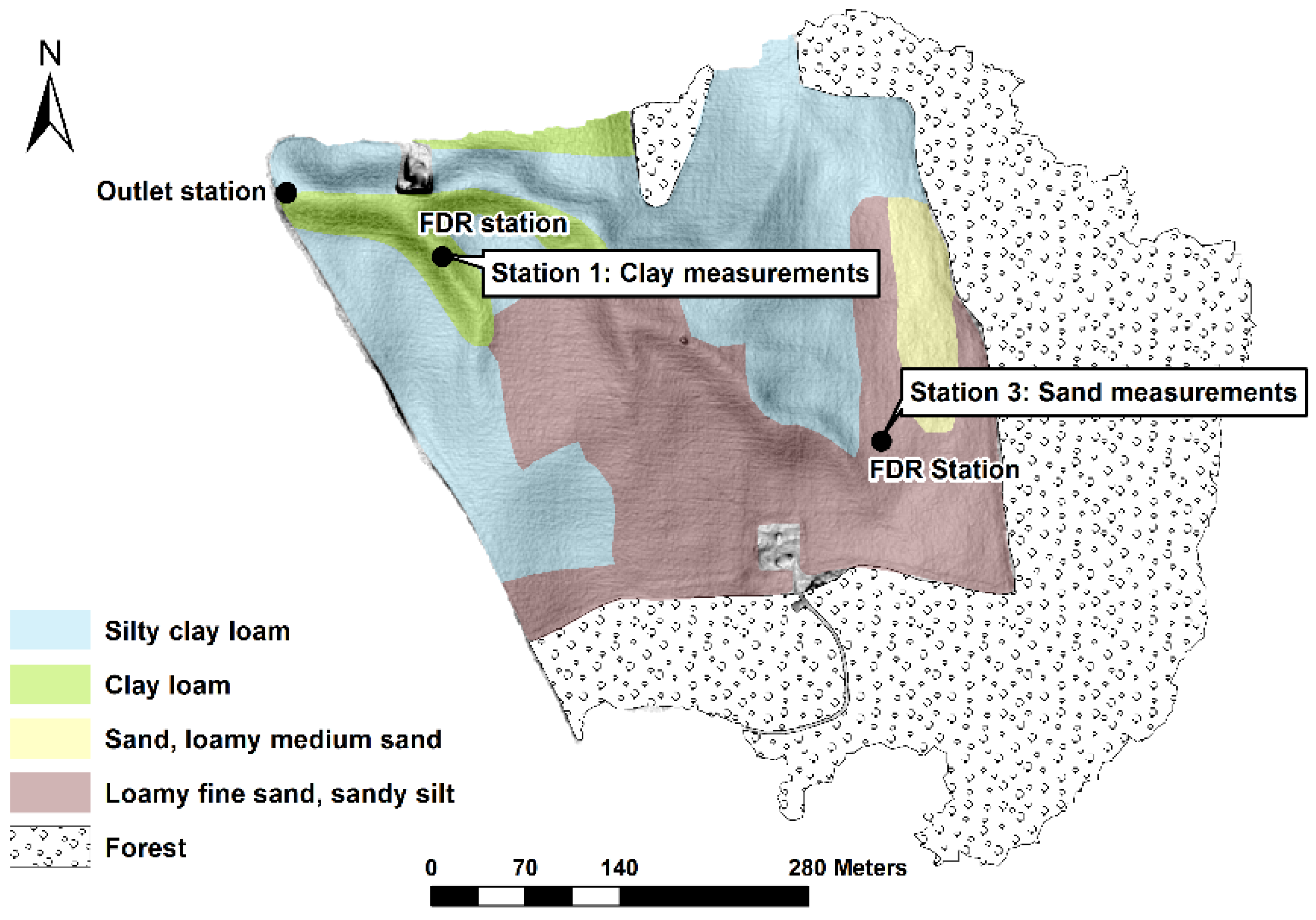
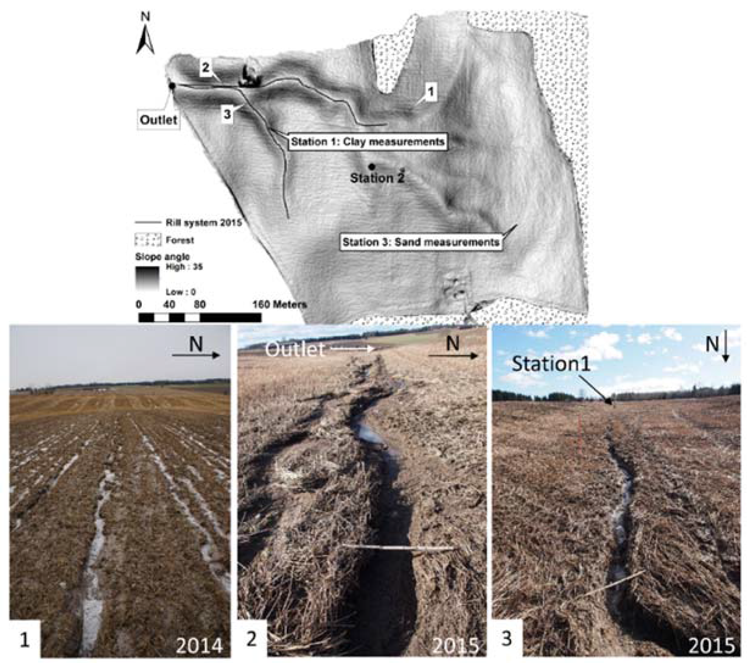
2.1. Study Area
2.2. Weather Data
2.3. Soil Temperature and Soil Moisture Measurements
2.4. Discharge Measurements
2.5. Snow Cover Properties
2.6. Erosion Mapping
2.7. SHAW Model Setup and Calibration
3. Results
3.1. Weather Measurements
3.2. Surface Discharge Measurements
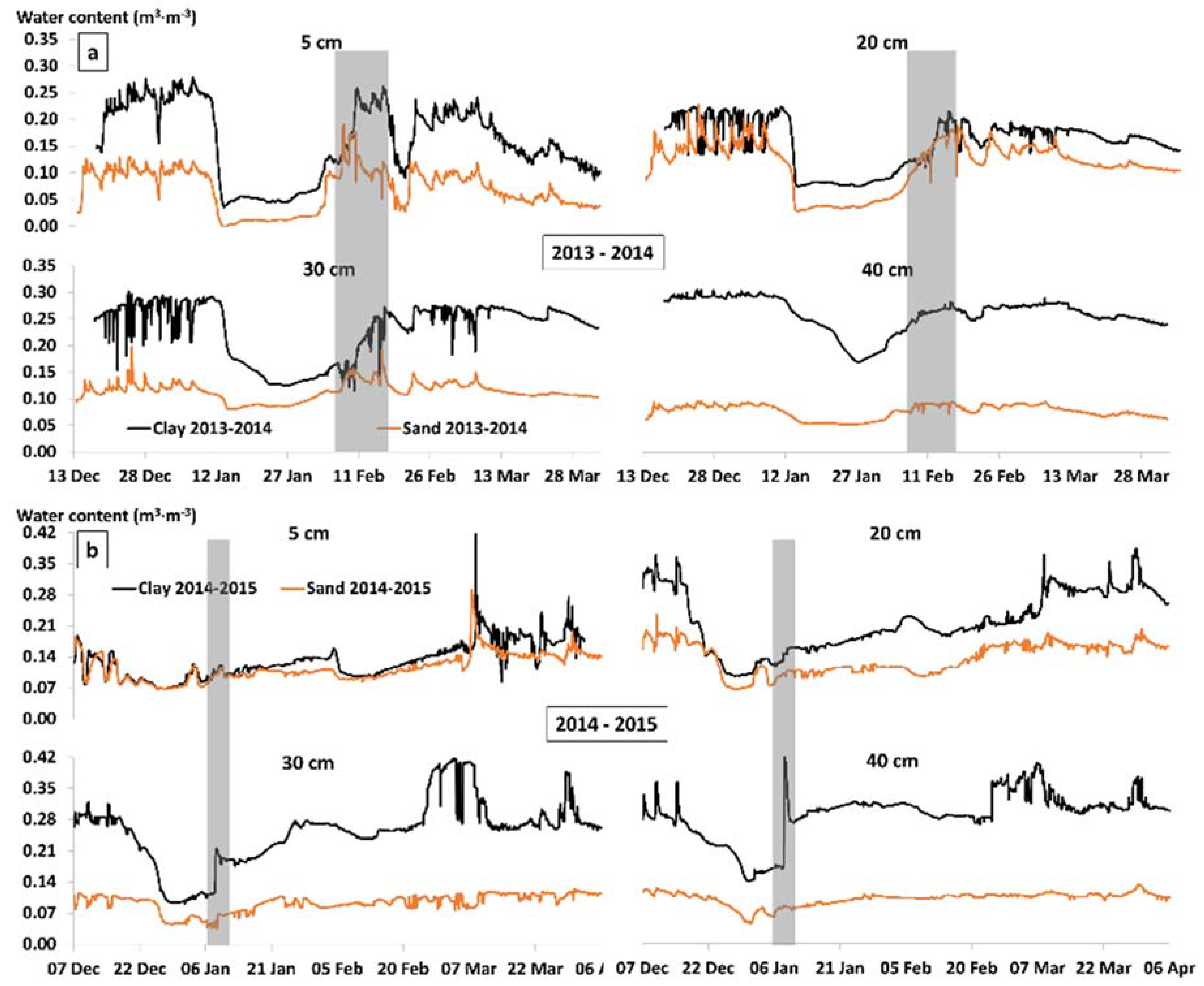
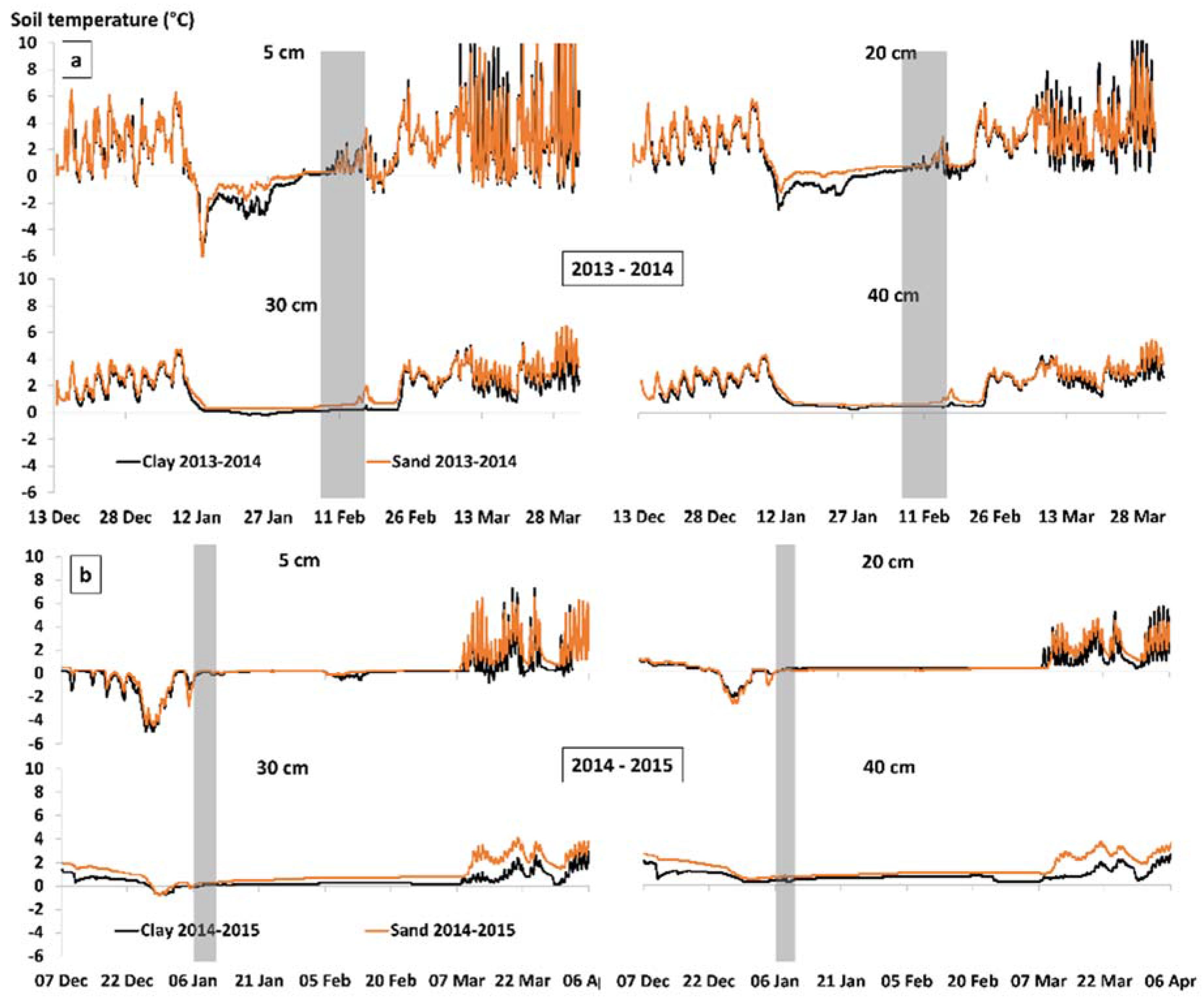
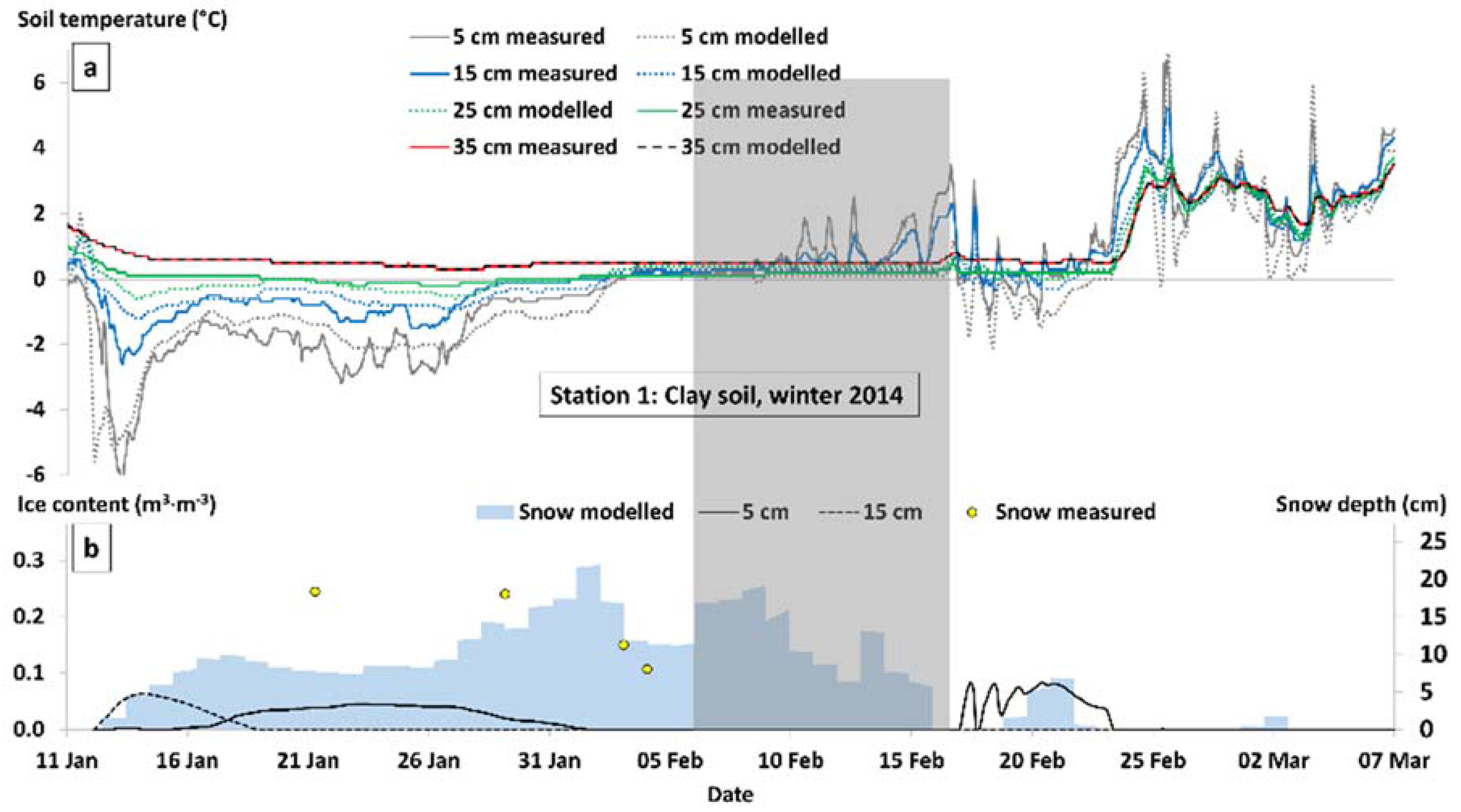
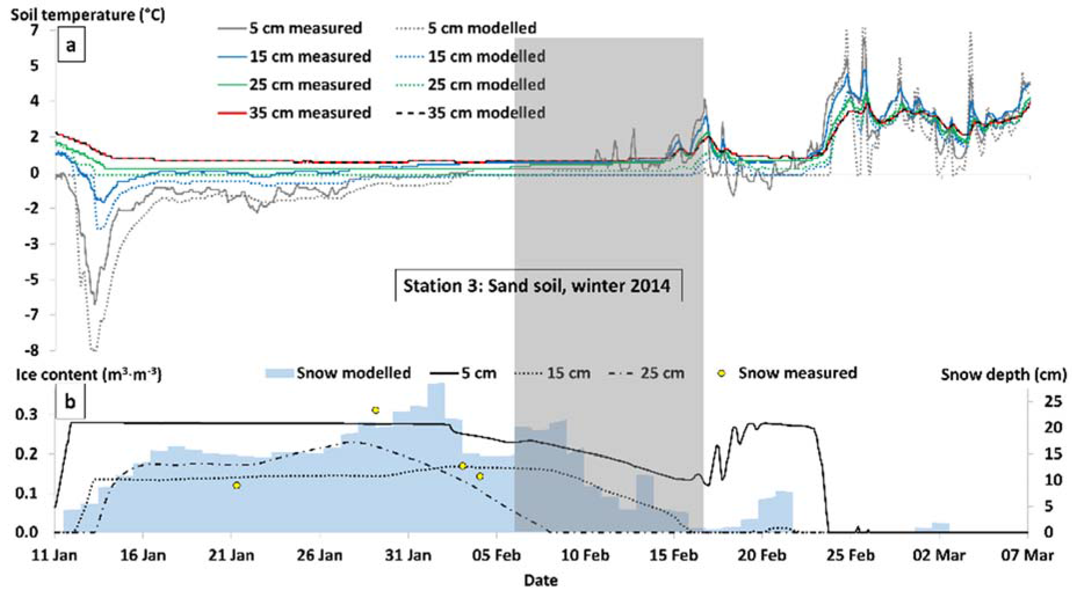
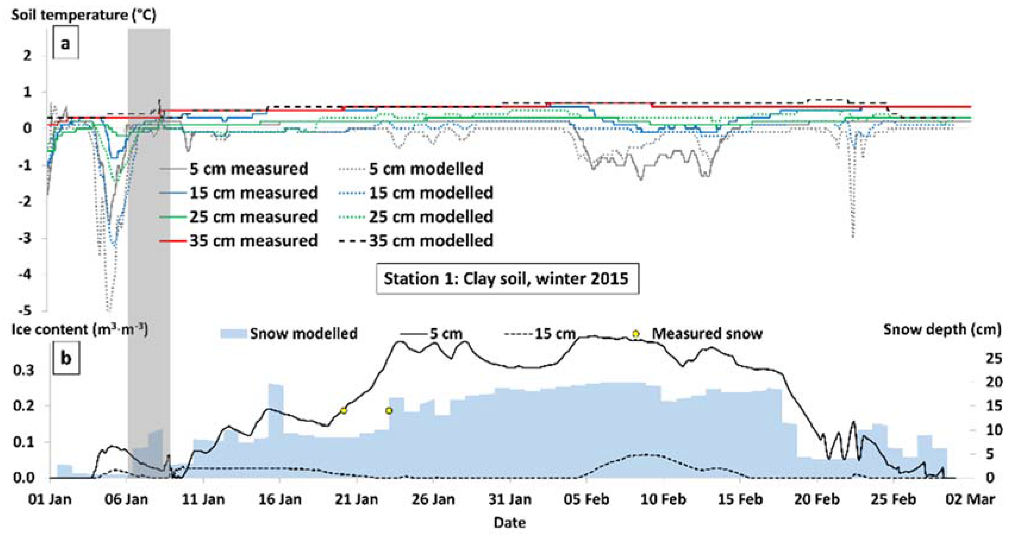
3.3. Liquid Soil Water Content and Soil Temperature
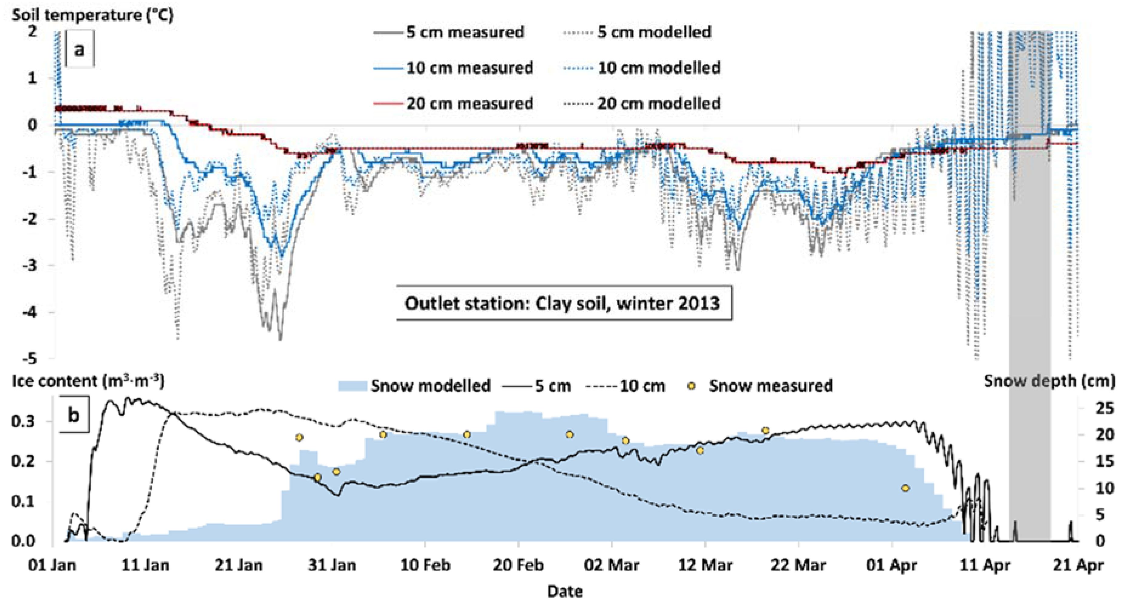
3.4. SHAW Modelling
3.5. Erosion Mapping
4. Discussion
5. Conclusions and Implications
Acknowledgments
Author Contributions
Conflicts of Interest
References
- Ollesch, G.; Sukhanovski, Y.; Kistner, I.; Rode, M.; Meissner, R. Characterization and modelling of the spatial heterogeneity of snowmelt erosion. Earth Surf. Process. Landf. 2005, 30, 197–211. [Google Scholar] [CrossRef]
- Iwata, Y.; Nemoto, M.; Hasegawa, S.; Yanai, Y.; Kuwao, K.; Hirota, T. Influence of rain, air temperature, and snow cover on subsequent spring-snowmelt infiltration into thin frozen soil layer in northern Japan. J. Hydrol. 2011, 401, 165–176. [Google Scholar] [CrossRef]
- Edwards, L.M.; Burney, J.R. Soil erosion losses under freeze/thaw and winter ground cover using a laboratory rainfall simulator. Can. Agric. Eng. 1987, 29, 109–115. [Google Scholar]
- Ban, Y.; Lei, T.; Liu, Z.; Chen, C. Comparison of rill flow velocity over frozen and thawed slopes with electrolyte tracer method. J. Hydrol. 2016, 534, 630–637. [Google Scholar] [CrossRef]
- Watanabe, K.; Kito, T.; Dun, S.; Wu, J.Q.; Greer, R.C.; Flury, M. Water Infiltration into a Frozen Soil with Simultaneous Melting of the Frozen Layer. Vadose Zone J. 2013, 12. [Google Scholar] [CrossRef]
- Yami, E.R.; Khalili, A.; Rahimi, H.; Etemad, A. Investigation of moisture on soil temperature regimes and frost depths in a laboratory model. Int. J. Agric. Sci. 2012, 2, 717–732. [Google Scholar]
- Al-Houri, Z.M.; Barber, M.E.; Yonge, D.R.; Ullman, J.L.; Beutel, M.W. Impact of frozen soils on the performance of infiltration treatment facilities. Cold Reg. Sci. Technol. 2009, 59, 51–57. [Google Scholar] [CrossRef]
- Willis, W.O.; Carlson, C.W.; Alessi, J.; Haas, H.J. Depth of freezing and spring run-off as related to fall soil-moisture level. Can. J. Soil Sci. 1961, 41, 115–123. [Google Scholar] [CrossRef]
- Stähli, M.; Nyberg, L.; Mellander, P.; Jansson, P.; Bishop, K.H. Soil forst effects on soil water and runoff dynamics along a boreal transect: 2. Simulations. Hydrol. Process. 2001, 15, 927–941. [Google Scholar] [CrossRef]
- Nyberg, L.; Stähli, M.; Mellander, P.; Bishop, K.H. Soil frost effect on soil water and runoff dynamics along a boreal forest transect: 1. Field investigations. Hydrol. Process. 2001, 15, 909–926. [Google Scholar] [CrossRef]
- Lindström, G.; Löfvenius, M.O. Tjäle Och Avrinning i Svartberget—Studier Med HBV-Modellen; SMHI hydrologi Nr 84; SMHI: Norrköping, Sweden, 2000. [Google Scholar]
- Iwata, Y.; Hayashi, M.; Suzuki, S.; Hirota, T.; Hasegawa, S. Effects of snow cover on soil freezing, water movement, and snowmelt infiltration: A paired plot experiment. Water Resour. Res. 2010, 46, 1–11. [Google Scholar] [CrossRef]
- Zhao, Y.; Nishimura, T.; Hill, R.; Miyazaki, T. Determining Hydraulic Conductivity for Air-Filled Porosity in an Unsaturated Frozen Soil by the Multistep Outflow Method. Vadose Zone J. 2013, 12. [Google Scholar] [CrossRef]
- Sutinen, R.; Hänninen, P.; Venäläinen, A. Effect of mild winter events on soil water content beneth snowpack. Cold Reg. Sci. Technol. 2008, 51, 56–67. [Google Scholar] [CrossRef]
- Zhao, Y.; Huang, M.B.; Horton, R.; Liu, F.; Peth, S.; Horn, R. Influence of winter grazing on water and heat flow in seasonal frozen soil of Inner Mongolia. Vadose Zone J. 2013, 12. [Google Scholar] [CrossRef]
- Parkin, G.; von Bertoldi, A.P.; McCoy, A.J. Effect of tillage on Soil Water Content and Temperature under Freeze-Thaw Conditions. Vadose Zone J. 2013, 12. [Google Scholar] [CrossRef]
- He, H.; Dyck, M.F.; Si, B.C.; Zhang, T.; Lv, J.; Wang, J. Soil freezing—Thawing characteristics and snowmelt infiltration in Cryalfs of Alberta, Canada. Geodermal. Reg. 2015, 5, 198–208. [Google Scholar] [CrossRef]
- Kormos, P.R.; Marks, D.; Williams, C.J.; Marshall, H.P.; Aishlin, P.; Chandler, D.G.; McNamara, J.P. Soil, snow, weather, and sub-surface storage data from a mountain catchment in the rain-snow transition zone. Earth Syst. Sci. Data 2014, 6, 165–173. [Google Scholar] [CrossRef]
- Williams, C.J.; Mcnamara, J.P.; Chandler, D.G. Controls on the temporal and spatial variability of soil moisture in a mountainous landscape: The signature of snow and complex terrain. Hydrol. Earth Syst. Sci. 2009, 13, 1325–1336. [Google Scholar] [CrossRef]
- Shanley, J.B.; Chalmers, A. The effect of frozen soil on snowmelt runoff at Sleepers River, Vermont. Hydrol. Process. 1999, 13, 1843–1857. [Google Scholar] [CrossRef]
- Lundekvam, H.; Skøien, S. Soil erosion in Norway. An overview of measurements from soil loss plots. Soil Use Manag. 1998, 14, 84–89. [Google Scholar] [CrossRef]
- Deelstra, J.; Kværnø, S.H.; Granlund, K.; Sileika, A.S.; Gaigalis, K.; Kyllmar, K.; Vagstad, N. Runoff and nutrient losses during winter periods in cold climates—Requirements to nutrient simulation models. J. Environ. Monit. 2009, 11, 602–609. [Google Scholar] [CrossRef] [PubMed]
- Øygarden, L. Rill and gully development during an extreme winter runoff event in Norway. Catena 2003, 50, 217–242. [Google Scholar] [CrossRef]
- Grønsten, H.A.; Lundekvam, H. Prediction of surface runoff and soil loss in southeastern Norway using the WEPP Hillslope model. Soil Tillage Res. 2006, 85, 186–199. [Google Scholar] [CrossRef]
- Flerchinger, G.N.; Xiao, W.; Sauer, T.J.; Yu, Q. Simulation of within-canopy radiation exchange. NJAS Wagening. J. Life Sci. 2009, 57, 5–15. [Google Scholar] [CrossRef]
- Hansen, N.C.; Gupta, S.C.; Moncrief, J.F. Snowmelt runoff, sediment, and phosphorous losses under three different tillage systems. Soil Tillage Res. 2000, 57, 93–100. [Google Scholar] [CrossRef]
- Govers, G. Rill erosion on arable land in central Belgium: Rates, controls and predictability. Catena 1991, 18, 133–155. [Google Scholar] [CrossRef]
- Boardman, J.; Shepheard, M.L.; Walker, E.; Foster, I.D.L. Soil erosion risk-assessment for on- and off-farm impacts: A test case using the Midhurst area, West Sussex, UK. J. Environ. Manag. 2009, 90, 2578–2588. [Google Scholar] [CrossRef] [PubMed]
- Weigert, A.; Schmidt, J. Water transport under winter conditions. Catena 2005, 64, 193–208. [Google Scholar] [CrossRef]
- Yakutina, O.P.; Nechaeva, T.V.; Smirnova, N.V. Consequences of snowmelt erosion: Soil fertility, productivity and quality of wheat on Greyzemic Phaeozem in the south of West Siberia. Agric. Ecosyst. Environ. 2015, 200, 88–93. [Google Scholar] [CrossRef]
- Su, J.J.; van Bochove, E.; Thériault, G.; Novotma, B.; Khaldoune, J.; Denault, J.T.; Zhou, J.; Nolin, M.C.; Hu, C.X.; Bernier, M.; et al. Effects of snowmelt on phosphorus and sediment losses from agricultural watersheds in Eastern Canada. Agric. Water Manag. 2011, 98, 867–876. [Google Scholar] [CrossRef]
- Kramer, G.J.; Stolte, J. Cold-Season Hydrologic Modeling in the Skuterud Catchment. An Energy Balance Snowmelt Model Coupled with a GIS-Based Hydrology Model; Bioforsk Report 4(126); Bioforsk: Ås, Norway, 2009; Volume 46. [Google Scholar]
- Thue-Hansen, V.; Grimenes, A.A. Meteorologiske Data for Ås; Norges Miljø og Biovitenskaplige Universitet: Ås, Norway, 2013–2014. [Google Scholar]
- Kværnø, S.H.; Øygarden, L. The influence of freeze-thaw cycles and soil moisture on aggreagte stability of three soils in Norway. Catena 2006, 67, 175–182. [Google Scholar] [CrossRef]
- Starkloff, T.; Stolte, J.; Hessel, R.; Ritsema, C. Understanding snowpack development at catchment scale, using comprehensive field observations and spatially distributed snow modelling. Hydrol. Res. 2017, in press. [Google Scholar]
- Flerchinger, G.N.; Saxton, K.E. Simultaneous heat and water model of a freezing snow-residue-soil system. I. Theory and development. Trans. Am. Soc. Agric. Eng. 1989, 32, 565–571. [Google Scholar] [CrossRef]
- Li, R.; Shi, H.; Flerchinger, G.N.; Akae, T.; Wang, C. Simulation of freezing and thawing soils in Inner Mongolia Hetao Irrigation District China. Geoderma 2012, 173, 28–33. [Google Scholar] [CrossRef]
- Flerchinger, G.N. The Simultaneous Heat and Water (SHAW) Model: Technical Documentation; Technical Report NWRC 2000-09; Northwest Watershed Research Center, USDA Agricultural Research Service: Boise, ID, USA, 2000.
- Black, C.A.; Evans, D.D.; White, J.L.; Ensminger, L.E.; Clark, F.E. Methods of Soil Analysis Physical and Mineralogical Properties, Including Statistics of Measurement and Sampling; American Society of Agronomy: Madison, WI, USA, 1965; Part 1; Volume 9, pp. 1–770. [Google Scholar]
- Flerchinger, G.N.; Sauer, T.J.; Aiken, R.A. Effects of crop residue cover and architecture on heat and water transfer at the soil surface. Geoderma 2003, 116, 217–233. [Google Scholar] [CrossRef]
- McCauley, C.A.; White, D.M.; Lilly, M.R.; Nyman, D.M. A comparison of hydraulic conductivities, permeabilities and infiltration rates in frozen and unfrozen soils. Cold Reg. Sci. Technol. 2002, 34, 117–125. [Google Scholar] [CrossRef]
- Øygarden, L.; Kværner, J.; Jenssen, P.D. Soil erosion via preferential flow to drainage systems in clay soils. Geoderma 1997, 76, 65–86. [Google Scholar] [CrossRef]
- Lundberg, A.; Ala-Aho, P.; Eklo, O.; Klöve, B.; Kværner, J.; Stumpp, C. Snow and frost: Implications for spatiotemporal infiltration patterns—A review. Hydrol. Process. 2015, 30, 1230–1250. [Google Scholar] [CrossRef]
- Boardman, J.; Poesen, J. Soil Erosion in Europe; John Wiley & Sons Inc.: Hoboken, NJ, USA, 2006; p. 855. [Google Scholar]


| Soil Type | Clay | Sand | ||||||
|---|---|---|---|---|---|---|---|---|
| Location | 59°40′ N, North Facing (22.5°), Slope 12°, Elevation ASL 100 m | 59°40′ N, Northwest Facing (330.5°), Slope 0°, Elevation ASL 140 m | ||||||
| Surface | Albedo of dry soil: 0.15 Wind profile surface roughness: 0.1 cm | |||||||
| Depth | 5 cm * | 15 cm * | 25 cm * | 35 cm | 5 cm | 15 cm | 25 cm | 35 cm |
| Campbell’s b | 20 | 20 | 20 | 20 | 3 | 1 | 1 | 1 |
| Air entry potential (hPa) | −31 | −31 | −34 | −35 | −31 | −31 | −34 | −35 |
| Ksat (cm·h−1) | 2.60 | 1.86 | 1.00 | 0.60 | 16.80 | 18.00 | 22.00 | 24.00 |
| Bulk density (kg·m−3) | 1331 | 1400 | 1535 | 1537 | 1190 | 1346 | 1346 | 1347 |
| θS | 0.40 | 0.40 | 0.40 | 0.35 | 0.43 | 0.40 | 0.40 | 0.31 |
| Sand (%) | 13 | 70 | ||||||
| Silt (%) | 58 | 13 | ||||||
| Clay (%) | 29 | 7 | ||||||
| Organic matter content (%) | 4.5 | 4.0 | 3.7 | 3.5 | 3.4 | 3.4 | 2.7 | 2.0 |
| Date | Total (mm) | Main Event | Highest Intensity (mm·h−1) |
|---|---|---|---|
| 14–19 April 2013 | 42.1 | 15.8 mm in 2 h | 9.3 |
| 6–16 February 2014 | 105 | 10 mm in 4 h | 4.6 |
| 6–8 January 2015 | 28 | 7 mm in 4 h | 2.0 |
| Date | Discharge (m3) | Precipitation (m3) | Discharge Coefficient (%) |
|---|---|---|---|
| 14–19 April 2013 | 3096 | 12,180 | 25 (50) |
| 6–16 February 2014 | 1008 * | 30,450 | 4 * |
| 6–8 January 2015 | 2594 | 8120 | 32 (63) |
© 2017 by the authors. Licensee MDPI, Basel, Switzerland. This article is an open access article distributed under the terms and conditions of the Creative Commons Attribution (CC BY) license ( http://creativecommons.org/licenses/by/4.0/).
Share and Cite
Starkloff, T.; Hessel, R.; Stolte, J.; Ritsema, C. Catchment Hydrology during Winter and Spring and the Link to Soil Erosion: A Case Study in Norway. Hydrology 2017, 4, 15. https://doi.org/10.3390/hydrology4010015
Starkloff T, Hessel R, Stolte J, Ritsema C. Catchment Hydrology during Winter and Spring and the Link to Soil Erosion: A Case Study in Norway. Hydrology. 2017; 4(1):15. https://doi.org/10.3390/hydrology4010015
Chicago/Turabian StyleStarkloff, Torsten, Rudi Hessel, Jannes Stolte, and Coen Ritsema. 2017. "Catchment Hydrology during Winter and Spring and the Link to Soil Erosion: A Case Study in Norway" Hydrology 4, no. 1: 15. https://doi.org/10.3390/hydrology4010015