Hydrological Modelling Using a Rainfall Simulator over an Experimental Hillslope Plot

Abstract

Hydrological processes are complex to compute in hilly areas when compared to plain areas. The governing processes behind runoff generation on hillslopes are subsurface storm flow, saturation excess flow, overland flow, return flow and pipe storage. The simulations of the above processes in the soil matrix require detailed hillslope hydrological modelling. In the present study, a hillslope experimental plot has been designed to study the runoff generation processes on the plot scale. The setup is designed keeping in view the natural hillslope conditions prevailing in the Northwestern Himalayas, India where high intensity rainfall events occur frequently. A rainfall simulator was installed over the experimental hillslope plot to generate rainfall with an intensity of 100 mm/h, which represents the dominating rainfall intensity range in the region. Soil moisture sensors were also installed at variable depths from 100 to 1000 mm at different locations of the plot to observe the soil moisture regime. From the experimental observations it was found that once the soil is saturated, it remains at field capacity for the next 24–36 h. Such antecedent moisture conditions are most favorable for the generation of rapid stormflow from hillslopes. A dye infiltration test was performed on the undisturbed soil column to observe the macropore fraction variability over the vegetated hillslopes. The estimated macropore fractions are used as essential input for the hillslope hydrological model. The main objective of the present study was to develop and test a method for estimating runoff responses from natural rainfall over hillslopes of the Northwestern Himalayas using a portable rainfall simulator. Using the experimental data and the developed conceptual model, the overland flow and the subsurface flow through a macropore-dominated area have been estimated/analyzed. The surface and subsurface runoff estimated using the developed hillslope hydrological model compared well with the observed surface runoff for a rainfall intensity of 100 mm/h. The surface runoff hydrograph was very well predicted by the model, with correlation coefficient (R²) and Nash–Sutcliffe efficiency coefficient (E) as 0.95 and 0.91, respectively. The observed soil/macropore storage component was estimated with the help of water balance equation and compared with the model predicted macropore storage. The error in computing the soil/macropore storage was estimated as 0.38 mm i.e., 13%.

1. Introduction

A rainfall simulator is an important principal apparatus for the study of infiltration, soil erosion, surface runoff and sediment transport, as it allows rainfall-runoff generation under controlled and repeatable conditions. A rainfall simulator permits generation of the rainfall at a known depth and intensity in controlled manner. In country like India, which has an agriculture-dominated economy and where the increasing population is constantly exerting pressure on the land and water resources, this type of field experiment is very useful for the understanding of complex water resources systems, especially in the hilly terrain of the Himalayas. Quantification of hydrological process on the hilly terrain is much more complex than in plain areas [1]. The hillslope hydrology is mainly controlled by subsurface storm flow, saturation excess flow, overland flow, return flow and pipe storage. Field experiments using rainfall simulators for estimating these parameters are scant, specifically over hilly terrain of the Northwestern Himalayas.

In the study of rainfall-runoff response by using rainfall simulator, the main query that arises is whether runoff response generated with a rainfall simulator matches with the natural storms. Researchers worldwide have focused on relative results such as the fraction of surface and subsurface runoff. Two problems occur in relating the runoff losses from simulated and natural rainstorms: reproducing the kinetic energy of a specific storm with a simulator, and scaling-up the results from a small simulator to a watershed/basin. The best way to reproduce the kinetic energy of natural storms is to replicate the natural rainfall duration and intensity with the simulator. For this, one requires the historical rainfall climatology records to select the desirable rainfall duration and intensity for the simulation. A well-adopted procedure is to choose a defined precipitation intensity, then run the simulator till steady state runoff is achieved or for a specified time [2]. Moreover, in hillslope hydrological studies, the additional problem of the incorporation of macropore-dominated processes has to be tackled. Macropores are actually large soil pores that are usually greater than 0.08 mm in diameter. Macropores allow free movement of air and water by gravity [3]. Macropores provide habitat for soil organisms and plant roots can grow into them. The process of infiltration into macroporous soils is primarily controlled by the network, density, connectivity and depth-wise distribution of macropores. It is important to quantify soil macroporosity and trace the dominating flow paths within continuous soil macropores to interpret the underlying flow mechanisms. The experimentally-derived quantitative data of soil macroporosity can have wide range of applications in various study domains such as water quality monitoring and groundwater pollution assessment due to preferential leaching of solutes and pesticides, study of soil structural properties and infiltration behavior of soils, investigation of flash floods in rivers, and hydrological modelling of the watersheds [4]. To understand the flow behavior of infiltrated water in active macropore structures of saturated undisturbed soil columns, dye tracing experiments and subsequent digital image processing exercises were carried out for the experimental plot in the present study. The method provided quantitative information about average fraction of macropores and volume density in terms of stained path width with depth as a descriptive variable. There are field and modelling studies that have attempted to understand and incorporate the spatially dynamic nature of the macropore flow system [5]. In spite of this progress in conceptualizing and modelling the macropore flow at the larger hillslope or watershed scale, little has been done to examine the details of accurate flow networks at the scale of individual macropores or soil pipes.

Rainfall simulators have been used successfully in research on many aspects of water resources over the last 70 years. Adams et al. [6] performed an analysis of surface runoff generation source by using large-scale rainfall simulator experiments. They used field experiments results to calibrate the hydrological model and interpret the runoff mechanisms. Sheridan et al. [7] used a rainfall simulator to obtain a modified erodibility index which could be used to predict annual erosion rates for forest roads. Arnaez et al. [8] used a rainfall simulator to compare runoff and sediment production under distinct rainfall intensities in a vineyard plantation in Spain. Verbist et al. [9] obtained soil loss values in 10 plots with bare soil in the Coquimbo Region using rainfall simulator setup. It has been shown in prior studies that rainfall simulators should have the ability to produce controlled and reproducible artificial rainfall which represents natural conditions at a given location. Rainfall simulators were proven as a useful tool in representing the natural rainfall events with fast data acquisition and controllable spatio-temporal variability of intensity, duration and kinetic energy.

Several studies have been performed on rainfall simulators so far and same have been referred for the selection of the design of rainfall simulator and the type of nozzle, in the present study. There are basically two types of rainfall simulators described in the literature: (1) nozzle type; and (2) tube type. Nozzle-type rain drop producing devices are much more common compared to the tube-type drop formers due to portability, capability of producing variable intensity and wide distribution range. Humphry et al. [10] designed a rainfall simulator which is easy to operate and transport while maintaining the intensity, distribution and energy characteristics of the natural rainfall. A single 50WSQ nozzle was used, producing rainfall with a kinetic energy of 25 J/mm·m², which is 87% of that of natural rainfall, and a drop size of 1.8 mm diameter, with an intensity of 70 mm/h. In this design, the usage of water was also less due to use of single nozzle. Sousa and Siqueira [11] developed a cost-efficient rainfall simulator for urban hydrology studies. The developed rainfall simulator simulated the rainfall events with raindrops of median diameter (D₅₀) of 2.12 mm and kinetic energy (KE) of 22.53 J/mm·m². The designed rainfall simulator was able to simulate rainfall intensities from 40 mm/h to 182 mm/h with Christiansen’s uniformity coefficient (CUC), ranging from 68.3% to 82.2%. Pe’ rez Latorre et al. [12] designed two different rainfall simulators using full-cone jet nozzles (RS1) and plane-jet nozzles (RS2) to obtain different rainfall intensities with drop sizes and energies similar to natural rainfall. It was observed that the design using plane jets (RS2) provided a more realistic drop size distribution and lower cost than that using full-cone jet nozzle (RS1) for lower rainfall intensity experiments. Abudi et al. [13] designed a high accuracy rainfall simulator for runoff and soil erosion studies. The mean drop size was found to be 1.5 mm and energy flux was 76% of the energy flux expected for natural rainfall of same intensity. Bubenzer [14] and Meyer [15] used Veejet 80100 nozzles in rainfall simulators, which have the ability to simulate physical characteristics of natural rainfall with 80% accuracy. The main drawbacks for this design were its complexity and time-consuming mechanisms. Later on, Swanson [16], Foster et al. [17] and Moore et al. [18] developed a rotating boom type of rainfall spray simulator with the same Veejet nozzles. Improved designs with Veejet nozzles achieved a wide range of intensities, up to 130 mm/h. Shelton et al. [19], and Miller [20] enhanced the capability of rainfall simulators by introducing spraying systems fulljet cone nozzles that provided continuous application, a wide angle, and variable intensities by adjusting the valve openings. In spite of many differences in the design and capabilities of the simulators and nozzle types described above, there are certain characteristics anticipated in a rainfall simulator. Therefore, on the basis of vast application of rainfall simulators, Meyer [21] prepared a list of desirable rainfall characteristics such as fall velocity, drop-size distribution, kinetic energy, uniformity, and intensity. However, the desirable characteristics and rainfall simulator design largely depend on the operational requirements, plot sizes, portability and the cost [18].

The main objective of the study was to develop and test a hillslope hydrological model with integration of hillslope-dominated runoff generation processes such as subsurface storm flow, saturation excess flow, overland flow, return flow and pipe storage using rainfall simulator experiments. In this study, a rainfall simulator was installed in a hillslope experimental plot of an area measuring 50 m² and used to generate rainfall event of variable intensities. Kinetic energy and rain drop size was then calculated so as to match with the natural rainfall events. The experimental rainfall response was observed over a hillslope plot. A hillslope hydrological model was developed and tested for surface, subsurface runoff and other water balance components.

2. Materials and Methods

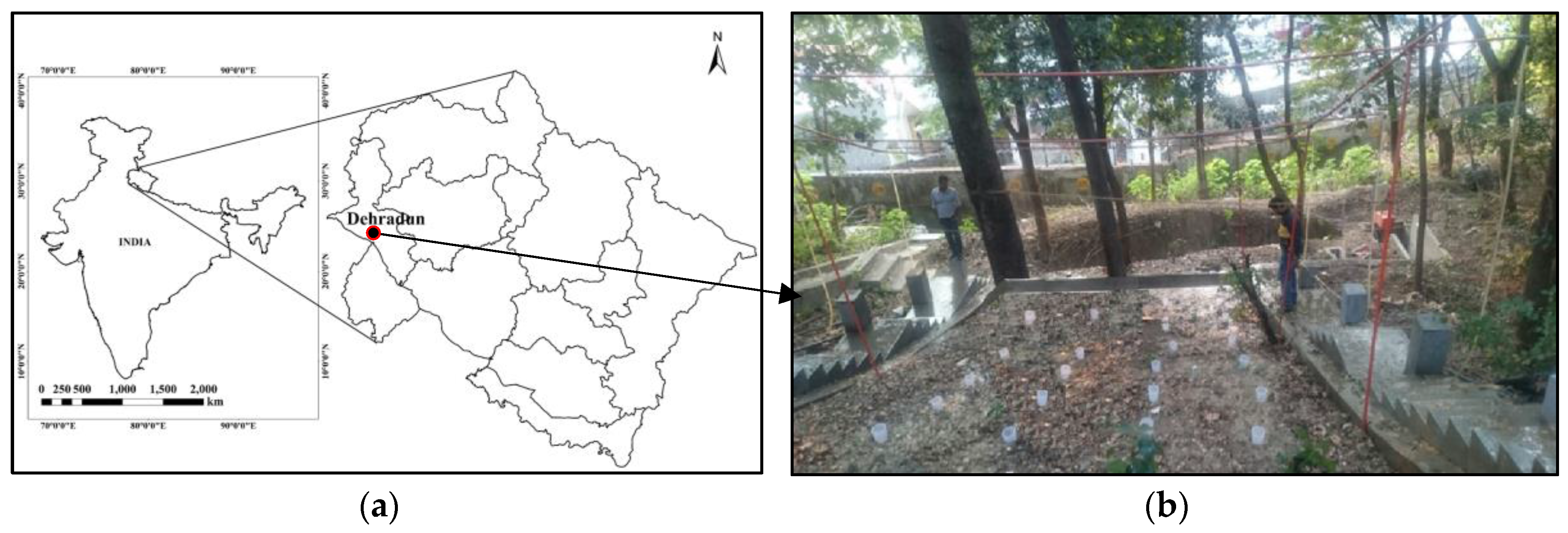
2.1. Study Area

The experimental hillslope site is located in the campus of Indian Institute of Remote Sensing, Dehradun, India at an elevation of 435 m above mean sea level. The average annual rainfall received in the area is around 2000 mm. The monsoon starts from June and continues until September. Around 70%–80% of annual rainfall occurs in the period of monsoon months and majority of this rain gets converted in to runoff due to terrain governed rainfall-runoff generation processes. To simulate rainfall-runoff generation processes, an experimental plot of 5 m × 10 m was developed. A detailed topographic survey of the experimental plot at a uniform grid of 0.05 m² has been done using a total station. The undisturbed soil samples were collected from the experimental plot (hillslope site) from top layer (0–10 cm) and bottom layer (10–30 cm). Bulk density test and soil texture analysis were done in the laboratory. The study area has loamy sand texture on top surface.

Table 1. Soil profile of plot area.

Soil Layer	Texture	% Sand	% Silt	% Clay	Bulk Density (g/cm3)
Top Layer (0–10 cm)	Loamy Sand	78.68	12.74	8.66	1.450
Bottom Layer (10–30 cm)	Loam	49.12	43.44	7.44	1.527

shows the soil characteristics of the experimental plot. The hard rock layer was observed at a varying depths starting from a depth of 0.5–1.2 m below the ground surface. Such an area can be highly conducive for quick subsurface flow generation under saturated conditions. A surface sealing effect is not applicable in these type of soils, as the infiltration rate is high and texture is loamy sand [22]. The experimental plot is covered with small shrubs throughout the year. The degree of vegetation depends on the climatic conditions. Figure 1(a-b) shows the location and image of experimental setup of hillslope plot.

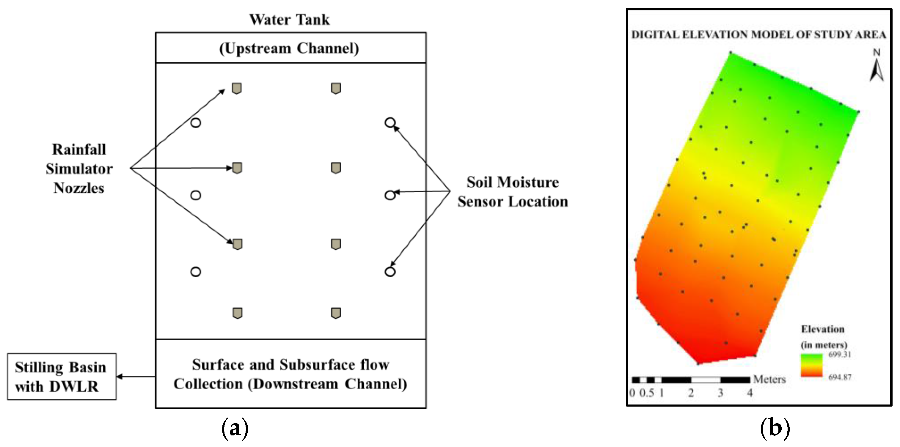
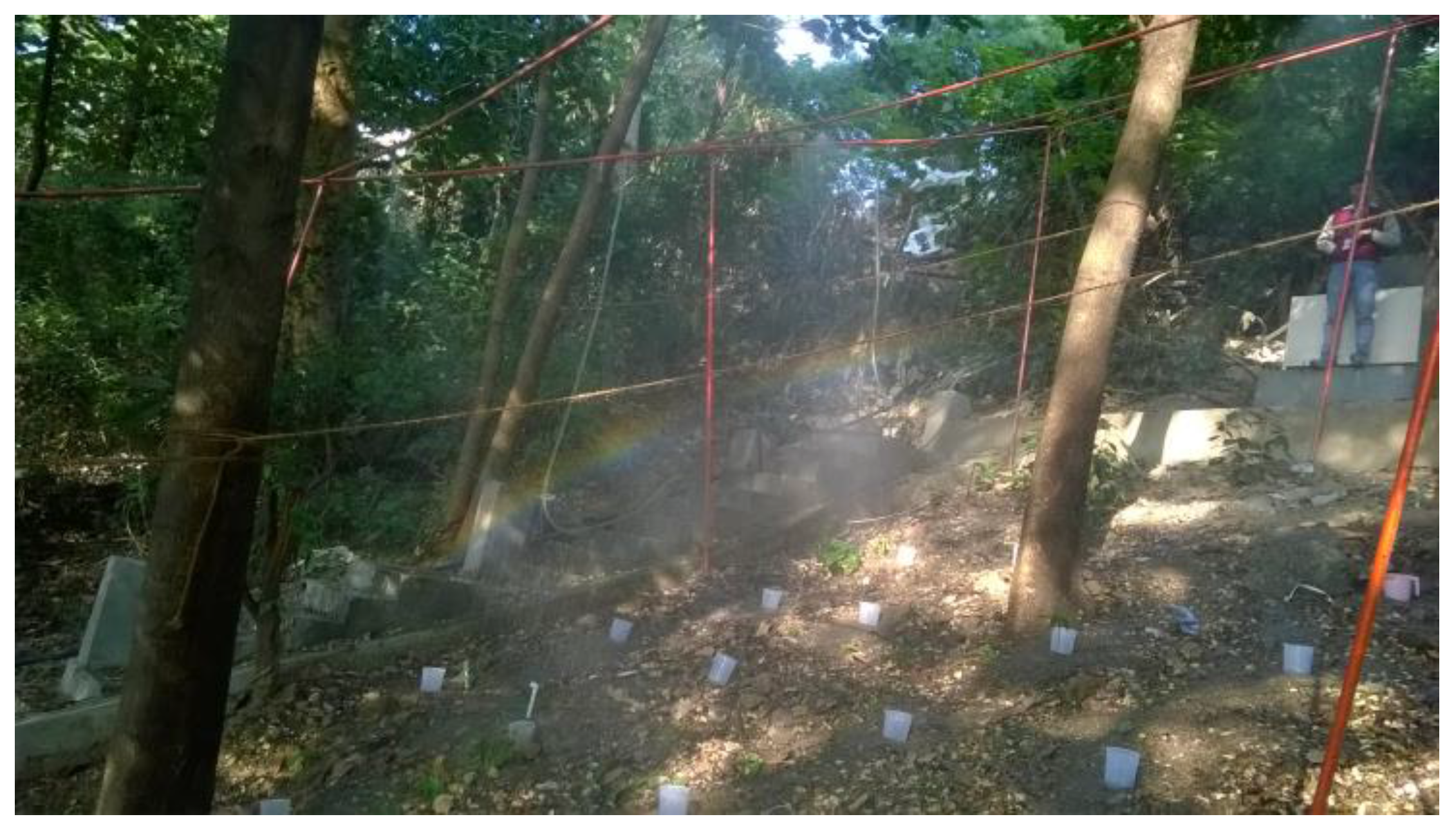
2.2. Rainfall Simulator Design

Our main purpose for designing a rainfall simulator was to enhance the uniformity and controllability over the previously designed rainfall simulators that would allow us to perform runoff studies in remote and difficult hilly terrain with more ease and less manpower. To make sure that designed rainfall simulator met the desirable technical requirements, the objective was fixed to develop the simulator that produces near natural rainfall characteristics such as median drop size, velocity, kinetic energy, intensity ranges, uniformity and continuity of flow.

On the basis of information available in peered review literature regarding size, type of nozzle and working mechanism of rainfall simulator, a portable rainfall simulator was fabricated at our laboratory, which is a continuous sprinkler system. The frame of the simulator was constructed from the 1.25-inch-diameter steel pipe and was installed on the experimental plot size of 5 m × 10 m. The simulator frame consisted of six legs made of steel pipe, three on each side. The legs were inserted into the ground to a depth of 30 cm and hinged with surrounded trees for the vertical support. Above the frame, four parallel pipes measuring 0.5 inches in diameter, with uniform spacing between them and each consisting of two nozzles and a pressure gauge, were connected. The parallel pipes are connected with the water supply pipes from both sides. The working setup of rainfall simulator is shown in Figure 1b.

The water supply system consists of two storage tanks, the first one that acts as primary tank, is of 10,000 L capacity. The water from this primary tanks is supplied to a small tank with a capacity of 400 L through gravity. This small tank is connected to a pump which supplies the water to both the pipes which are connected to the parallel pipes over the rainfall simulator frame. The nozzle system used on the simulator was the Spraying Systems Fulljet 1/2HH 50WSQ solid cone nozzle. Two nozzles were placed at the top of the frame on each 0.5-inch pipe, almost 3 m above the ground surface. The nozzle was threaded directly into the 0.5-inch pipe. The selection of the nozzle was done based on literature review for best possible replication of natural rainfall on the plot.

2.3. Experimental Setup and Investigations

For conducting the simulated rainfall experiments on the plot scale level, the experimental setup was designed keeping in view the natural hillslope conditions which are dominant in the Northwestern Himalayas. Keeping the above conditions in mind, an overland flow and subsurface flow collection system was set up at the experimental site. The intensity of rainfall was controlled with the help of the pressure gauges and pressure regulators installed at each parallel pipe on which nozzles were fixed. The simulator was designed in such a way that it covered the entire area of the test plot and distributed the rainfall equally and uniformly over the whole test plot area. Soil moisture sensors were also installed at different depths and locations to monitor the soil moisture variability before, during and after the rainfall simulation experiments.

To collect the runoff, a collecting channel with a gentle slope of 2% was constructed with H flume at the outlet of channel. The runoff water was diverted to the stilling basin where the digital water level recorder (DWLR) was installed to record the water level variations. Small holes were kept in the wall of the channel along the side of the plot and connected to collection tank through pipes to record the subsurface flow. A pump was used to feed the water from the upstream storage tank to the water distribution pipe network of a rainfall simulator. For uniform sprinkling of water through nozzles, proper pressure was maintained at each pressure gauge located at each top pipe. A schematic diagram of the experimental plot and digital elevation model of the experimental plot is shown in Figure 2. The digital elevation map has been presented in the paper to represent the hilly slope profile of the experimental plot. A portable rain gauge was also installed at the experimental site to continuously measure the intensity of the rainfall from simulator.

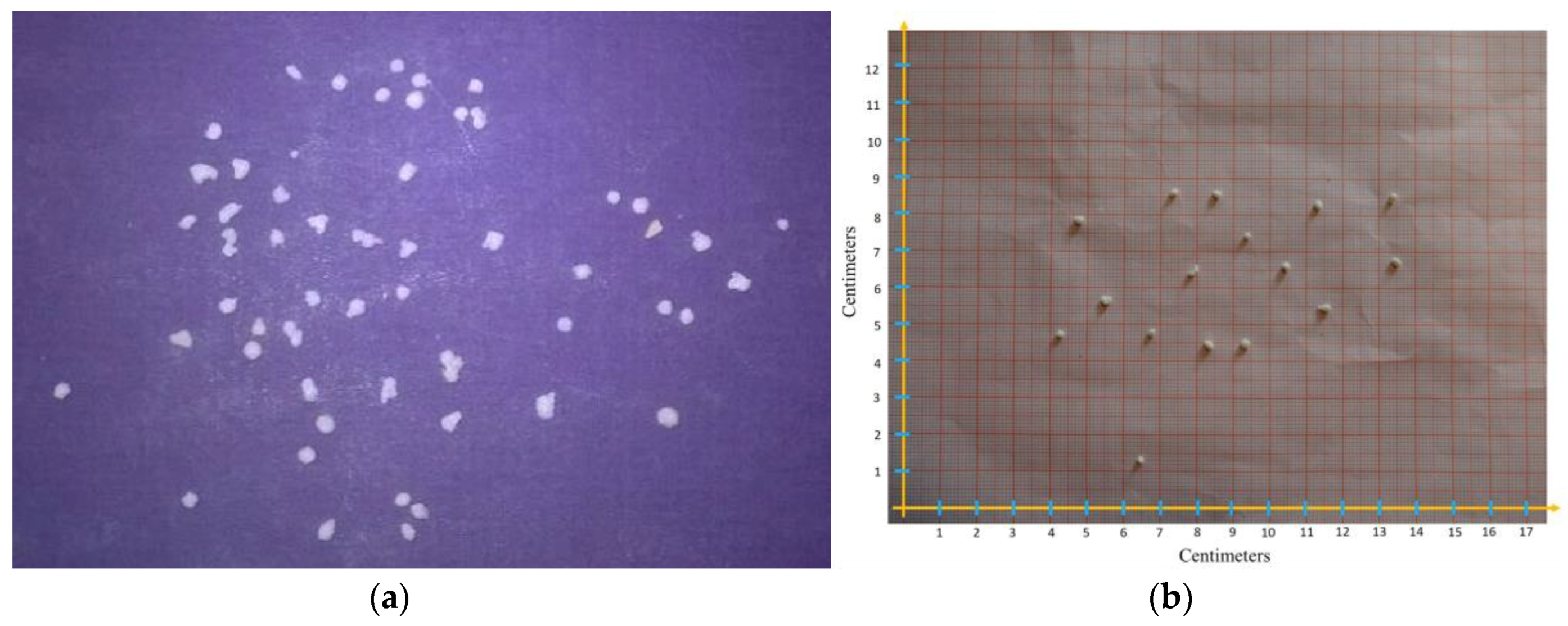
2.3.1. Raindrop Size Estimation

Raindrop characteristics play important role in many scientific, commercial and industrial applications [23]. The rainfall intensity is also related to the median raindrops diameter by a power function and hence knowledge of raindrop size becomes essential for understanding and modeling the hydrological process in the experimental plot. In this exercise, the drop-size distribution of simulated rainfall was determined by using the flour pellet method described by Hudson [24]. A tray of flour was exposed to simulated rainfall for a period of around 2 s. The flour was then dried for 24 h at room temperature (~28 °C) and the pellets formed as shown in Figure 3 were passed through a series of sieves (4.75, 3.35, 2.36, 1.18 and 0.85 mm). The distributed pellets were then dried for 24 h at 105 °C, weighed and measured. Drops smaller than 1 mm in diameter could not be produced, while those larger than 6 mm could not be determined accurately by this method. The results revealed that the rain drop size follows the gamma distribution and size varies between 1 mm to 5 mm for rainfall intensity 100 mm/h, while the 80% raindrop size lies between 2 to 4 mm, which is very noteworthy and assumed to be a replication of the natural rain storms.

2.3.2. Performance Evaluation of Rainfall Simulator

The uniformity of rainfall application to the field with rainfall simulator is usually reported as either the distribution uniformity (DU) or Christiansen’s uniformity coefficient (CUC) [25]. CUC is a widely used method of calculating the uniformity of water application from rainfall simulators and expressed in percentage as:

$$CUC=100(1-\frac{Averagedeviationfromaveragedepthofapplication}{Overallaveragedepthofapplication})\%$$

$$CUC=100(1-(\sum \left|x-\overline{x}\right|/\mathrm{n}\overline{x}))$$

(1)

where, n = no. of sample points; $x$ = rainfall (mm) at each point; and $\overline{x}$ = mean of x values.

Rainfall experiments were performed three times for 30 min with intensity 100 mm/h to check the uniformity of rainfall simulator. The simulated rainfall was collected in the 36 containers placed over the experimental plot at uniform grid of 1 m apart from each other. The capacity of each container was 600 mL. Figure 4 shows the setup of experiment conducted for estimation of coefficient of uniformity on the plot. The average CUC calculated was 79%, which is quite satisfactory on the plot of bigger size [26].

2.3.3. Estimation of Kinetic Energy and Velocity of Rainfall

The kinetic energy of rainfall is a widely used indicator of the potential ability of rain to detach soil. The empirical equation given by Wischmeier and Smith [27] for the kinetic energy of the raindrop is given as:

$$e=11.897+8.73{\log }_{10}\mathrm{I}$$

(2)

$$\mathrm{E}={{\displaystyle \sum }}_{i=0}^{n}e\times P$$

(3)

where, e is the kinetic energy (J/mm·m²); I is the rainfall intensity (mm/h); P is the rainfall amount (mm); E is the kinetic energy (J/m²); and n is the number of rainfall periods.

Basically, the kinetic energy of rainfall is estimated from the kinetic energy of each individual raindrop that strikes the ground surface. The drop-size distribution measurements along with fall velocity measurements or empirical laws linking fall velocity (v) and drop diameter (d), let one calculate the rain kinetic energy. Raindrop velocity is based on the raindrop diameter, which can be estimated by modified Newton’s equation.

$$\mathrm{v}=(17.20-0.84\mathrm{d})\times (\mathrm{d})\times 0.5$$

(4)

where, d is diameter of the raindrop.

The relation between drop velocity and drop size when compared with its terminal velocity given by Lows and Parson [28] is given in

Table 2. Comparison of measured raindrop velocity and terminal velocity with respect to drop diameter (Lows and Parson, 1943).

Drop Diameter (mm)	Terminal Velocity (m/s)	Velocity (m/s) Measured
1	4	3.3
1.5	5.3	4
2	6.5	5
2.5	7.2	5.7
3	8	6.2
3.5	8.5	6
more	≤9	-

.

2.3.4. Soil Macropore Characteristics

In order to quantify the macropore structures in the hillslopes, an undisturbed soil column was obtained from the study site. The soil column has a circular dimension with a diameter of 53 cm, which was extracted from the field plot using a steel ring of the same diameter and a depth of 30 cm. The initial wet conditions of the soil columns were obtained by continuously supplying the water for 1 h with a constant ponding depth of 3 cm. Then, the soil column was left for 4–5 h to attain field capacity. The dye test experiment was done after the soil attained the field capacity. The dye was applied for 1 h with a constant ponding depth of 3 cm. Then, the soil column was left for another 4–5 h for proper distribution of dye in soil column. Then, the steel ring was removed and soil column was sliced horizontally by a sharp edged thin plate at 2 cm intervals from the top to analyze the dye distribution patterns. The distortions in dye patterns due to slicing were negligible as the soils were not cohesive and had low water-holding capacity. A graduated frame was placed on the soil surface to provide a reference for the image analysis.

Digital images (nadir photographs) of each horizontal slice were taken using a digital SLR camera (Canon EOS 400D, 10 Mega Pixels resolution) for digital image analysis of the dye patterns. For accurate measurement of stained areas, the images were color corrected, digitally rectified, and scaled to a resolution of one square millimeter per pixel [29]. These corrected images were analyzed to determine the characteristics of macropore flow for the soils collected from the hillslope plot. The stained paths indicated flow paths with continuous macropore connectivity. The unstained pores that are visible on a horizontal slice are the macropores for which the connectivity was disturbed. Therefore, in relation to active macropore flow, the main area of interest was to quantify the stained path width and their distribution in both horizontal and vertical faces. After every image analysis, a classification report was generated to find the percentage coverage area of the dye in the soil slices. The image analysis of soil photographs provided the useful detail of the depth of the dye penetration. The dye penetration was visible up to the last sliced part of the soil. This indicates that the continuous macropores are present in the soil throughout the depth. This type of macropore connectivity is generally observed in the soils with densely vegetated roots. Figure 5 shows the subset images of the sliced soil columns, which were further used for digital image analysis to find out macropore characteristics of experimental plot. Fraction of macropore present at different soil depths were used as input and to calibrate the hillslope hydrological model.

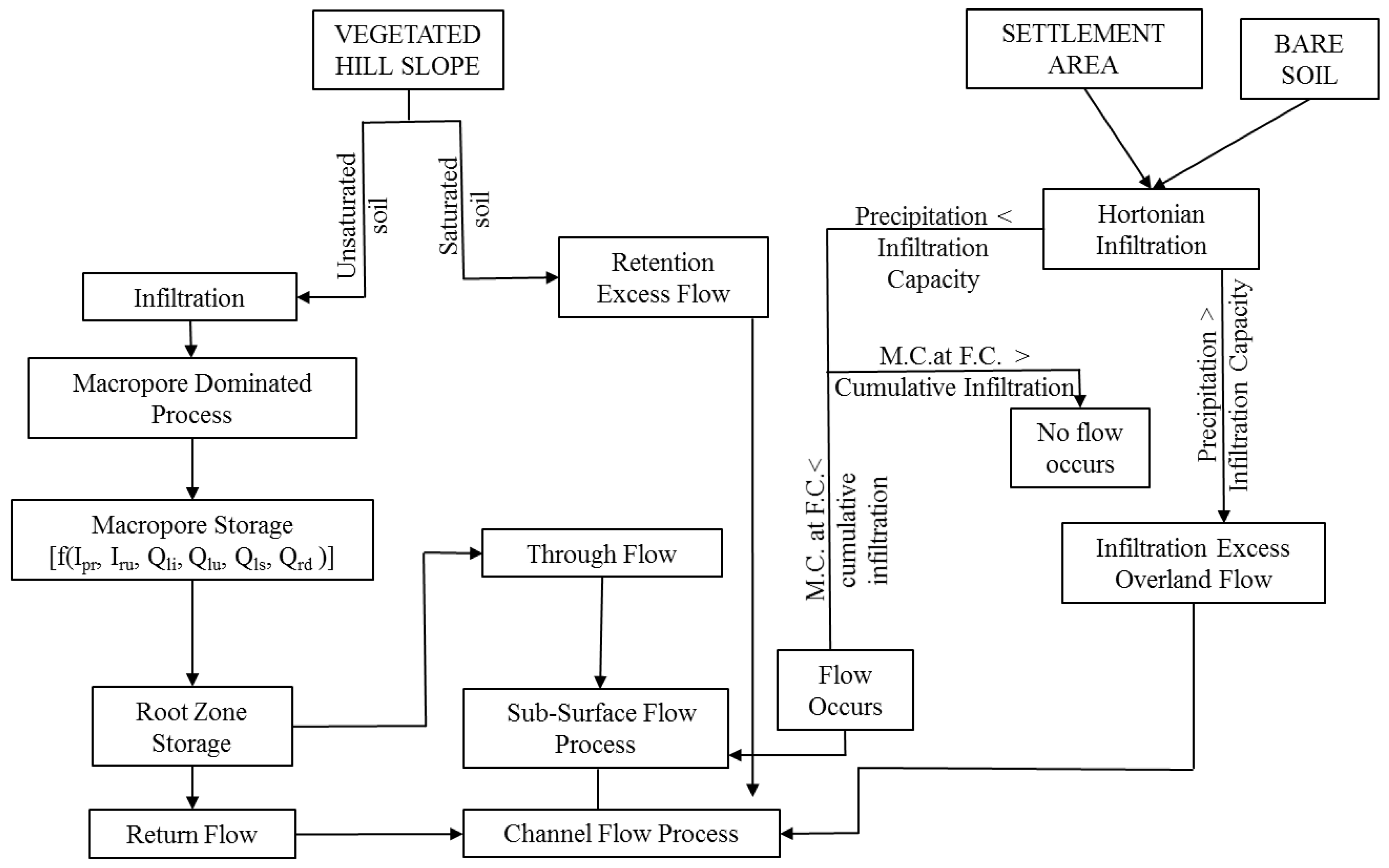
3. Hydrological Modeling

This part describes the hydrological model for the hillslope areas. The study area is conceptually divided into four hydrological similarity classes (HSC), namely, vegetated hillslope, agricultural field, settlement area and bare soil. The developed model framework is based on the physical processes on the hillslopes, where topmost surface layer interacts with the rainfall. At a hillslope site, surface runoff can be generated by any of three (1) infiltration excess; (2) saturation excess; or (3) variable source area processes [4]. If the soil is saturated, then saturation excess overland flow or retention excess flow occurs from the vegetated hillslope areas and the agriculture fields, most common near the toe of the slopes where the accumulated water from the entire hillslopes is enormous in volume [30]. The excess saturation excess water directly contributes to the channel flow and if the soil of the above two classes is partially saturated or un-saturated, then the rain water will infiltrate into soil and enter the macropore area causing the occurrence of macropore-dominated processes like subsurface flow, return flow (water that not consumed by soil root zone and throughflow but returned back to the surface due to excess pressure), throughflow (a subcomponent of interflow, is the lateral unsaturated flow of water in the soil zone) and pipe storage. Agnese et al. [31] derived a simple storage-based hillslope hydrological response model by assuming the quick runoff by surface runoff generation and compared the results with Horton’s theory of runoff generation. They argued that difficulties and complexity in estimating the local parameters cause model prediction errors. The overland flow is not a source of runoff generation in the forested watersheds [32]. Therefore, insight relating to macropore flow processes is most desirable in the recent scenario. Subsurface movement of water largely contributes to the storm runoff generation.

From macropore storage, surface water enters in the root zone storage from where it will be a part of return flow or throughflow depending on the root zone storage capacity. As name suggests, return flow directly contributes to the channel flow and the water from the throughflow adds to subsurface flow processes. The hydrological processes on the other two classes i.e., settlement area and the bare soil are based on the Hortonian infiltration excess runoff generation theory [33]. If the rainfall intensity is less than the infiltration capacity of the soil, then the water will be added to the subsurface flow while for the reverse case, infiltration excess flow will occur, which contributes to the channel flow. Total subsurface flow was calculated by adding the throughflow and the flow from Hortonian infiltration and the total channel flow was estimated by adding return flow, retention excess overland flow and infiltration excess overland flow. Freeze [34] discussed the importance of subsurface flow in generation of surface runoff in highland areas. Figure 6 shows the conceptual flow chart of hydrological processes and their interdependence in the hilly slope areas/hilly watersheds. Anderson et al. [32] and Dunne [35] performed several experiments to identify the dominant flow pathways and discuss the condition of occurrence of these flow paths.

Mathematical Framework of Hillslope Hydrological Model

The mechanism of infiltration in the hillslope area/hilly watershed is mainly controlled by macropores. Macropores initiate the subsurface stormflow after saturating the surrounding soil matrix. The water flow and balance equation for this condition is given by Kroes et al. [36] as:

$${\mathrm{S}}^{\mathrm{t}}-{\mathrm{S}}^{{\mathrm{t}}_0}={{\displaystyle \int }}_{\mathit{t}\mathbf{0}}^{\mathit{t}}(\mathit{I}\mathit{p}\mathit{r}+\mathit{I}\mathit{r}\mathit{u}+\mathit{Q}\mathit{l}\mathit{i}-\mathit{Q}\mathit{l}\mathit{u}-\mathit{Q}\mathit{l}\mathit{s})$$

(5)

where,

$${\mathrm{Q}}_{\mathrm{li}}={{\displaystyle \int }}_{\mathit{z},\mathit{i}\mathit{f},\mathit{b}\mathit{o}\mathit{t}}^{\mathit{z},\mathit{i}\mathit{f},\mathit{t}\mathit{o}\mathit{p}}{\mathit{Q}}_{\mathit{l}\mathit{i}};{\mathrm{Q}}_{\mathrm{lu}}={{\displaystyle \int }}_{\mathit{z},\mathit{u}\mathit{n}\mathit{s},\mathit{b}\mathit{o}\mathit{t}}^{\mathit{z},=\mathbf{0}}{\mathit{Q}}_{\mathit{l}\mathit{u}};{\mathrm{Q}}_{\mathrm{ls}}={{\displaystyle \int }}_{\mathit{z},\mathit{p}\mathit{r}\mathit{o}\mathit{f},\mathit{b}\mathit{o}\mathit{t}}^{\mathit{z},\mathit{u}\mathit{n}\mathit{s},\mathit{b}\mathit{o}\mathit{t}}{\mathit{Q}}_{\mathit{l}\mathit{s}}$$

The +ve terms represent infiltration into soil matrix, while the −ve term shows exfiltration from soil matrix. Depths z,if,top, z,if,bot, z,uns,bot and z,prof,bot (cm) refer to top and bottom of interflow zone, and bottom of unsaturated zone and soil profile, respectively and:

(1)

Storage of water in the main bypass domain of macropore S_mb (cm);

(2)

Infiltration of water into macropores at the soil surface, by precipitation, irrigation and snowmelt water falling directly into macropores I_pr and by overland flow (runoff) into the macropores I_ru (cm/d);

(3)

Lateral infiltration into the unsaturated soil matrix Q_lu (cm/d);

(4)

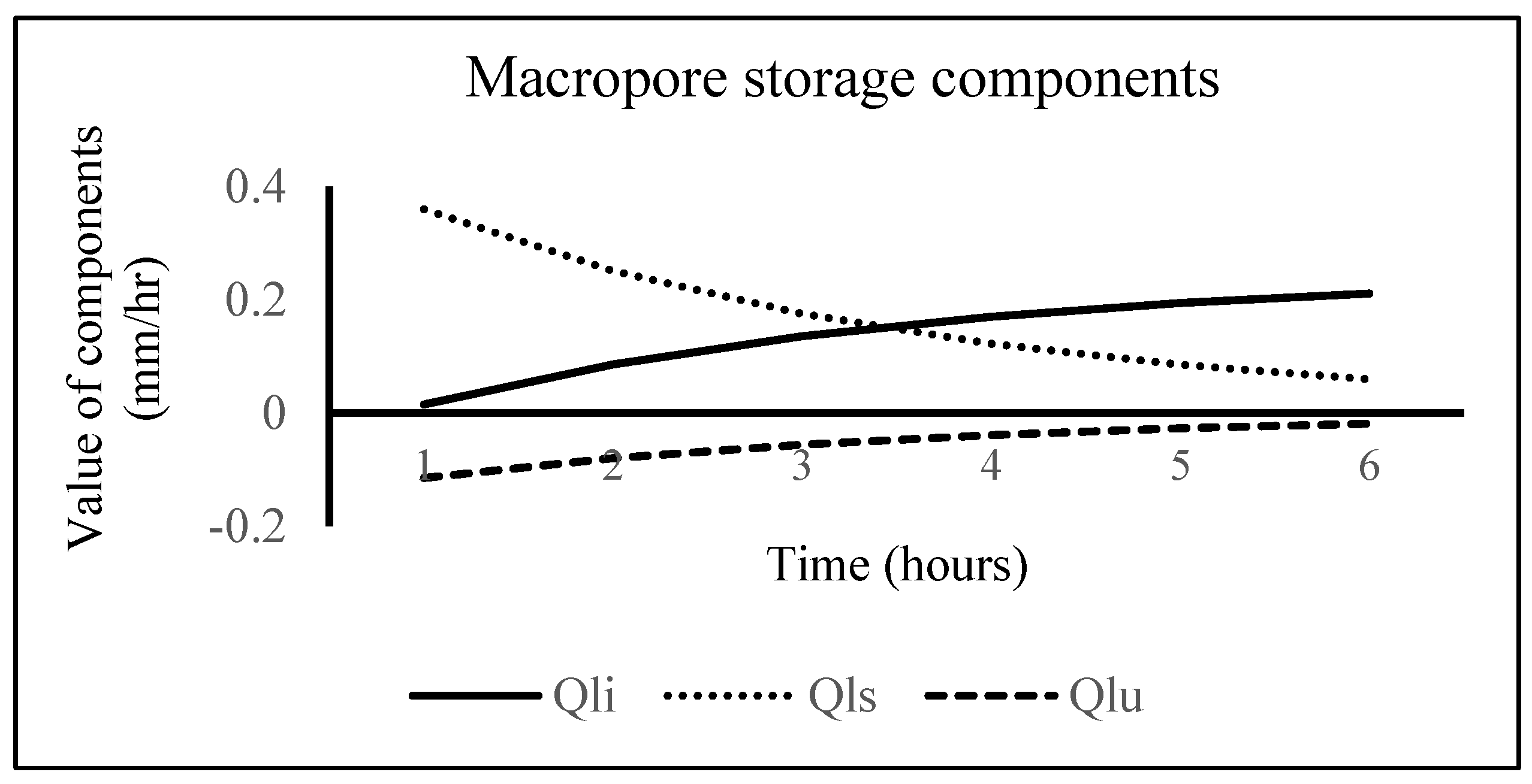
Lateral exfiltration out of the saturated soil matrix Q_ls (cm/d);

(5)

Lateral exfiltration out of the saturated soil matrix by interflow out of a zone with perched groundwater Q_li (cm/d).

The rate of precipitation I_pr, irrigation and snowmelt water routed directly into the macropores at the soil surface at a given precipitation/irrigation/snowmelt intensity P (cm/d) is calculated as:

I_pr = A_mp × P

(6)

where, A_mp (cm²/cm²) is the horizontal macropore area fraction at the soil surface which equals V_mpo (cm³/cm³), the total macropore volume fraction at soil surface.

Ponding occurs when the total of precipitation, irrigation and inundation intensity exceed soil matrix infiltration capacity and subsequently, overland flow occurs. Infiltration rate I_ru due to overland flow or surface runoff is numerically given as:

I_ru = h_o/ϒ_Iru

(7)

where, h_o is the pressure head at the soil surface which is equal to the ponding height in cm and ϒ_Iru is the resistance of macropore inflow at soil surface. Lateral infiltration of macropore water into the unsaturated soil matrix (Q_lu) takes place strictly over the depth where stored macropore water is in contact with the unsaturated matrix. Absorption is the dominant mechanism at low soil moisture content. It will be negligible under wet conditions even when there is a large pressure head gradient and for this condition, Darcy flow will be dominant. Darcy flow is very small under dry conditions because of very low hydraulic conductivities.

Using a one-dimensional flow equation combined with Darcy’s equation [37], the lateral infiltration can be computed as:

Q_lu = S_r/2t^−1/2

(8)

where, S_r is the sorptivity, which is computed by using Young’s estimation formula as:

S_r = 6.3 (θ − θ_r)^0.5 K_sat^0.25

(9)

where, θ is the moisture content at the present time, θ_r is the residual moisture content i.e., moisture content at wilting point, and K_sat is the saturated hydraulic conductivity.

Lateral exfiltration out of saturated soil matrix water into the macropores (Q_ls), only concerns static macropores below the groundwater table, since in the present concept in case of the saturated condition the soil is assumed to be swollen to its maximum volume. The lateral exfiltration rate per unit of depth Q_ls, (cm/cm.d) in the case of water-filled macropores (Pressure head (h_mp) > 0) is described by Darcy flow:

Q_ls = f_shp × 8 × K_sat × (h_mp − h_mt)/(d²_pol)

(10)

where, h_mp and h_mt are the pressure head in the water-filled macropores and in the unsaturated soil matrix, respectively.

Parameter f_shp is a shape factor to account for the uncertainties in the theoretical description of lateral infiltration by Darcy flow originating from uncertainties in the exact shape of the soil matrix polygons. Theoretically, the value of f_shp lies between 1 and 2. Infiltration occurs if h_mp > h_mt and exfiltration if h_mp < h_mt.

Lateral exfiltration out of the saturated matrix as interflow (Q^*_li) is a special case of exfiltration of soil water from the saturated zone into the macropores and is described as:

Q^*_li = −(f_shp × 8 × K_sat × (h_mp − h_mt)/(d²_pol))

(11)

If h_mp > h_mt, infiltration into the saturated matrix in the perched groundwater zone occurs. Here, perched groundwater is defined as the subsurface water that forms a saturated horizon within porous media at an elevation higher than the local or regional groundwater table, d_pol is the effective diameter of soil polygon which is nothing but the macropore diameter and is given by:

d_pol = d_p,min + (d_p,max − d_p,min) × (1 − M)

(12)

where, d_p,min and d_p,max are the minimum and maximum diameter of the macropores, M is the relative macropore density which is the ratio of the static macropore volume to the static macropore volume at surface.

Retention excess flow (Q_re) occurs if the soil is already saturated. The main factor affecting this flow is the availability of soil moisture content. The retention excess flow can be calculated as:

Q_re = P − I

(13)

where, P is the rainfall intensity in mm/h and I is the infiltration capacity in mm/h.

Return flow (saturation overland flow) occurs where the soil is completely saturated and no additional water can be accepted into soil. This type of flow is most common near the toe of the slopes where the accumulated water from the entire hillslopes is enormous in volume. This is a time-dependent condition i.e., the longer the rainfall occurs, the more water will be in the soil layers, and hence a greater area will be subjected to saturation. This flow returns to the land surface after flowing a short distance in the upper soil horizon. Return flow per unit length at the hillslope can be calculated using the following equation:

Q_return = H_o V_lat (L − L_s)

(14)

where, Q_return is the return flow (mm/day), and H_o is the saturated thickness normal at the hillslope outlet expressed as function of total thickness (mm/mm). V_lat is the velocity of the flow at the outlet (mm/day) which can be defined as:

V_lat = K_s sin (α)

(15)

where, α is the hillslope angle.

Throughflow is the downslope flow of water occurring physically within soil surface under unsaturated condition. Throughflow can maintain both low flows (baseflow) in rivers by low subsurface drainage and also contribute to high peak flows (stormflow) through its role in generating saturation excess overland flow. In this study, throughflow is calculated as the difference between the root zone storage and the return flow.

Through flow = S_rz − Return flow

(16)

where, S_rz is the root zone storage.

The above process will occur in the areas with vegetated hillslopes and agriculture land. For the areas covered with settlement and the bare soil, two scenarios occur. The first refers to when the rainfall intensity is less than infiltration capacity. In this case, the water directly infiltrates into the soil and contributes to the subsurface flow. In the second case i.e., when rainfall intensity is higher than infiltration capacity, infiltration excess overland flow occurs. This flow is also known as Hortonian flow and occurs mainly in irrigated areas, urban areas and generally during the storms with very high intensity of rainfall. The infiltration excess overland flow is calculated by Horton’s equation which is given as:

f_p = f_c + (f₀ + f_c) e^−kt

(17)

where, f_p is the infiltration capacity (depth/time) at some time t, k is constant depending on soil characteristics and vegetative cover, f_c is a final or equilibrium capacity, and f₀ is the initial infiltration capacity.

Rainfall event was simulated for the rainfall intensity 100 mm/h by maintaining the nozzle pressure to around 82 kPa through pressure regulators installed in the water distribution network of the rainfall simulator [38]. Each of the experiments was repeated three times for 30 min. Hence, a total of nine rainfall simulations were conducted in three months. Each set of simulation was started only after ensuring that the surface soil moisture in the experimental plot was equal to the soil moisture of the nearby area outside the experimental plot (to resemble with the natural condition). The surface runoff was collected in the channel and measured with the help of digital water level recorder installed at the end of channel. Subsurface flow was collected through the runoff collection mechanisms as discussed in Section 2.3.

The observed rainfall and soil characteristics were given as input parameters into the developed hillslope hydrological model to estimate the surface, subsurface flow and other macropore flow components. Then, the simulated and observed values of surface and subsurface flow for the experimental plot were compared and performance of the model was tested.

4. Results and Discussion

4.1. Field Observations

The typical characteristics of the hillslopes, climate, and hydro-geologic conditions prevailing in the Northwestern Himalayas have been elaborated in previous section in order to justify the adoption of the experimental techniques. A detailed description of the experimental setup and the methodologies for the in-situ observations were also provided previously along with description of instrumentation used in the hillslope plot and the data captured from artificial storm events. The observed field data and the results obtained from the simulated rainfall event with an intensity of 100 mm/h have been discussed in detail to draw suitable inferences about the hydrological response of the hillslope plot.

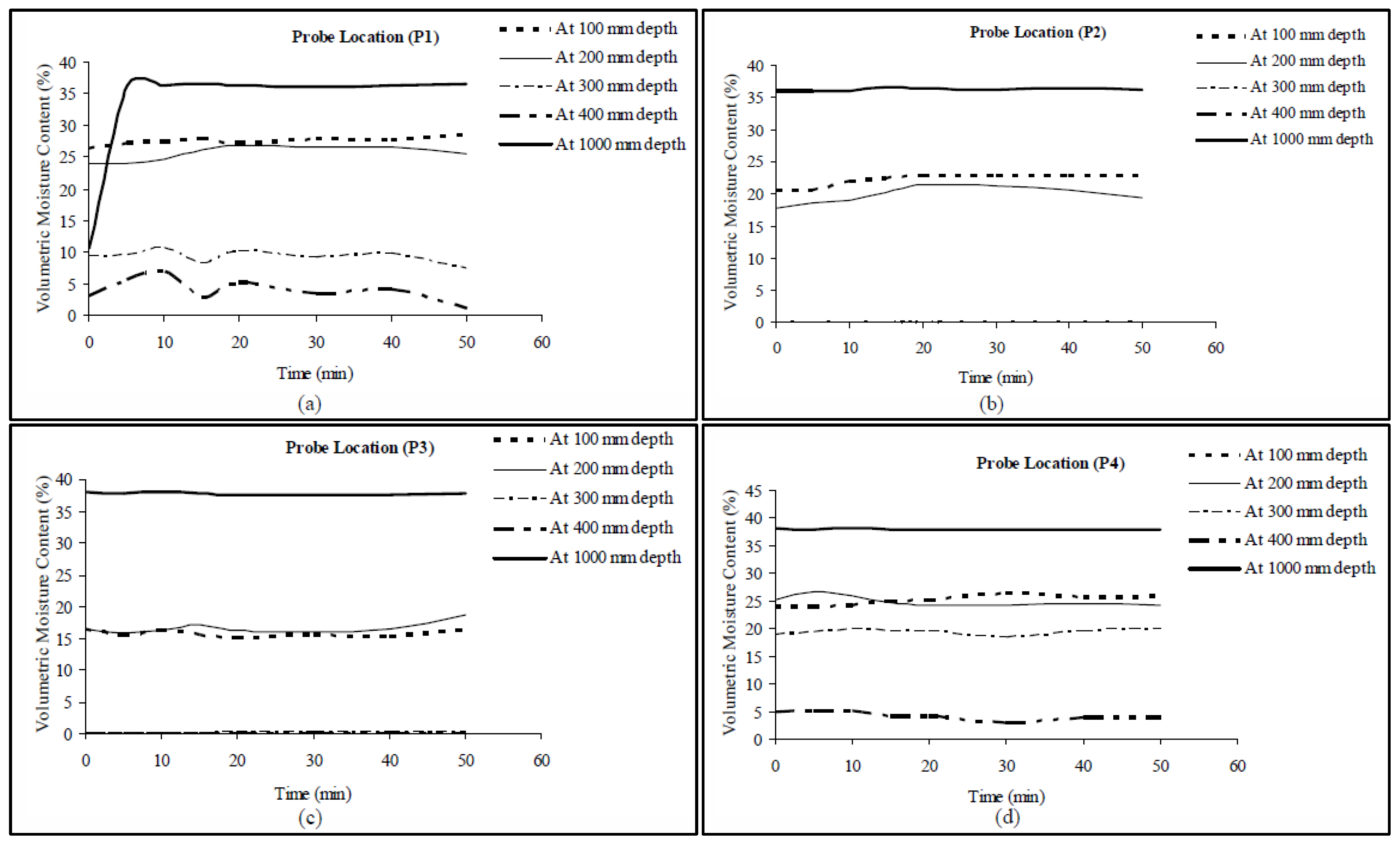
4.1.1. Study of Soil Moisture Profile in the Hillslope Plot

Temporal variations of soil moisture profile within the hillslope plot before, during, and after the rainfall-runoff experiments were precisely monitored using the profile probe soil moisture sensors. Interesting observations could be made from the soil moisture patterns in the hillslope soil. The graphs in Figure 7a–d clearly show that once a wet antecedent moisture condition is attained, the moisture content of soils at different depths remains almost constant during the rainfall-runoff events as well as after the cessation of surface runoff. It can be observed that the constant soil moisture conditions over the plot have been attained very quickly during the runoff event. This is a very important finding related to the present investigation. Figure 7a–d shows temporal variations in soil moisture content at different depths (below ground level) in the hillslope plot during and immediately after the runoff experiment.

Figure 7a–d clearly depicts that after a wet antecedent condition has been established, the moisture content in the top soil layer does not vary. Rainfall experiments were started after ensuring the resemblance of soil moisture to the natural condition outside the experimental plot. The soil moisture variations for the middle layer (300 mm and 400 mm) for probe location P2 and P3 could not be captured due to a technical fault at the sensor level. However, the middle layer soil (300–400 mm) for probe location P1 and P4 shows relatively low but stable moisture content. Temporal variations of the soil moisture profiles at the probe location P1 at a depth of 1000 mm indicate that the infiltrated water bypasses this layer to reach the bottom layer where the buildup of water table takes place over the impermeable bed and causes lateral diversion of water in the form of subsurface stormflow. Such bypassing flow patterns within the soil combined with rapid buildup and recession of water table in the hillslope soil profile strongly indicates the existence of highly active lateral preferential pathways in the subsoil. However, the quick rise of soil moisture at probe location P2, P3 and P4 might be due to the vertical drainage along the installed soil moisture probe.

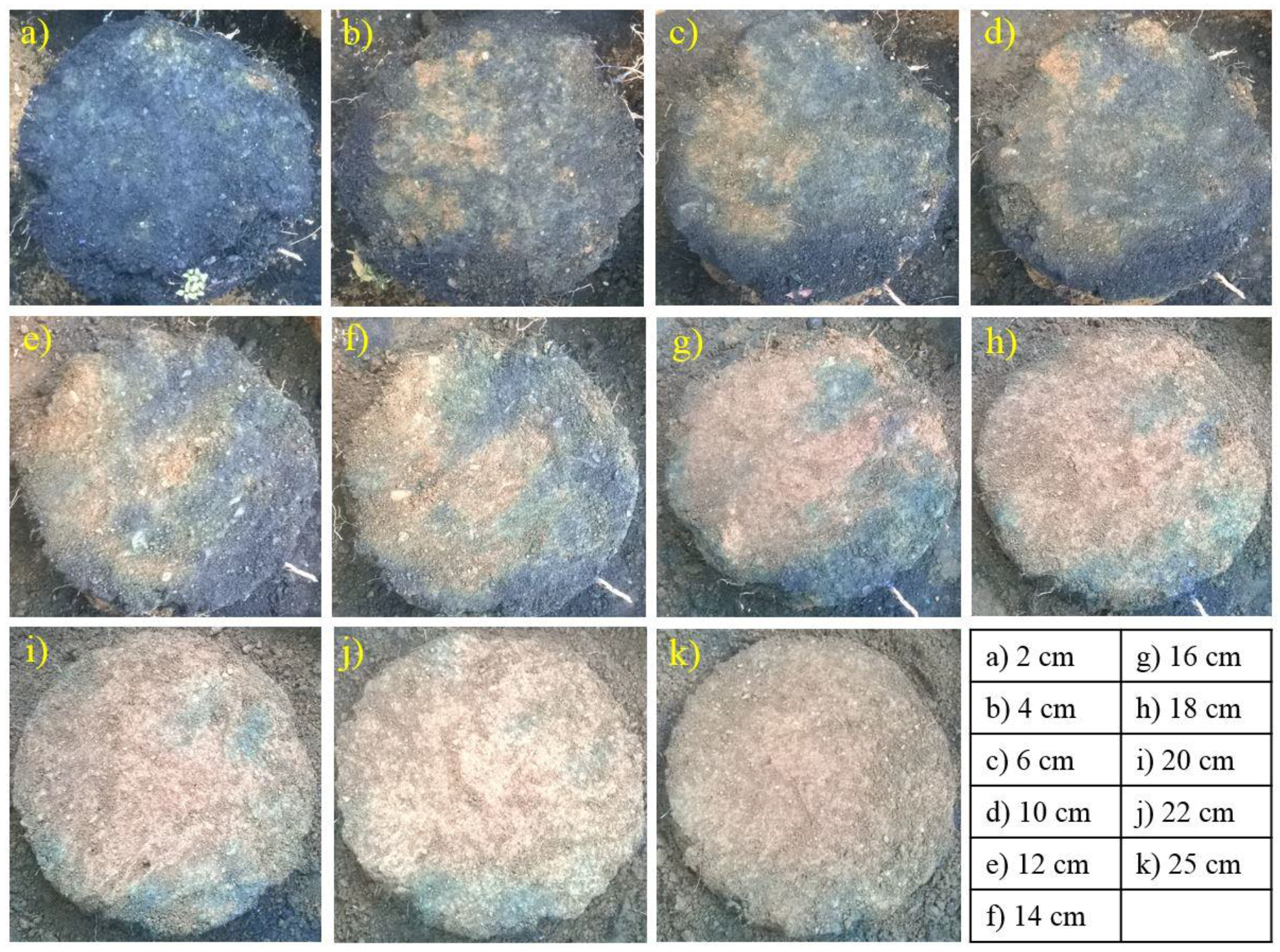
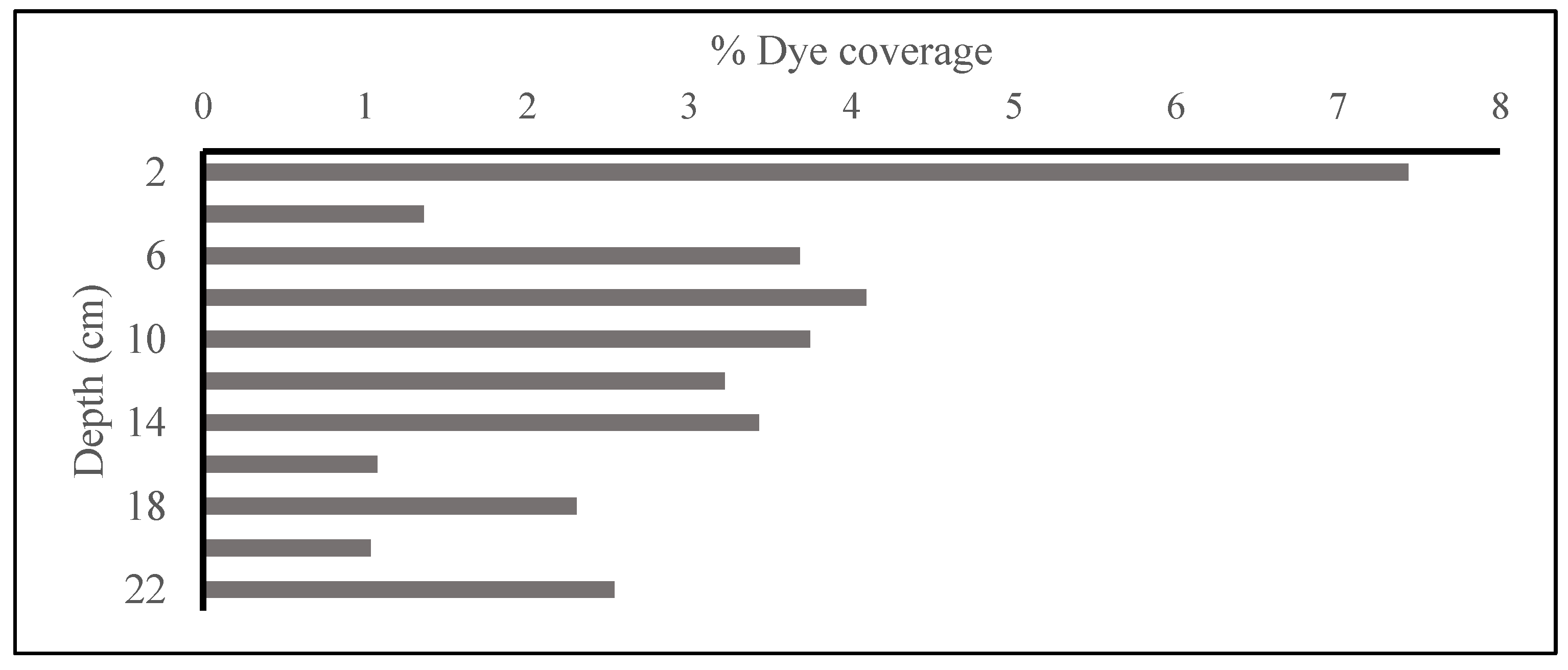
4.1.2. Results of Dye Pattern Analysis

The horizontal dye patterns provide detailed information about the maximum depth of dye penetration and percentage dye coverage of the sections. Percentage dye coverage versus depth was plotted for the soil column. Figure 8 shows the depth-wise distribution of percentage dye coverage for the hillslope soil column. The soil column had maximum dye coverage of 7.41% at a 2-cm·depth and an average of 3.08%. In the soil column, the color dye penetration was clearly visible up to the last soil layer. This indicates the presence of continuous macropores throughout the soil column. Such distribution of macropores can be expected from densely vegetated undisturbed hillslope soils where growth of plant roots provides connectivity to preferential pathways for water movement. The occurrence of maximum dye coverage within a 14-cm·depth also represents higher root density and activity of soil fauna and flora in the top soil layer. From the average dye coverage, it can be noted that most of the flow pathways were concentrated to 3.08% of total area in soil column. These results justify the demand of dedicated hydrological model for hilly-slope areas having capability of handling macropore-dominant processes as is done by the model implemented in the present study.

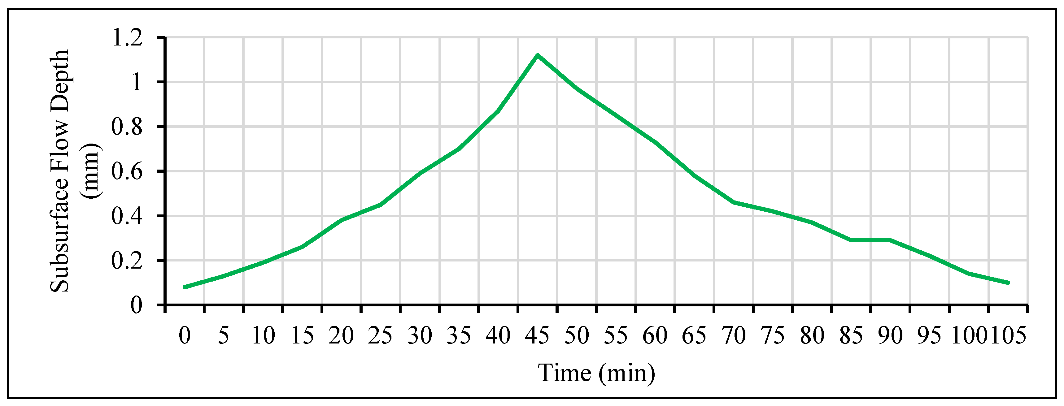
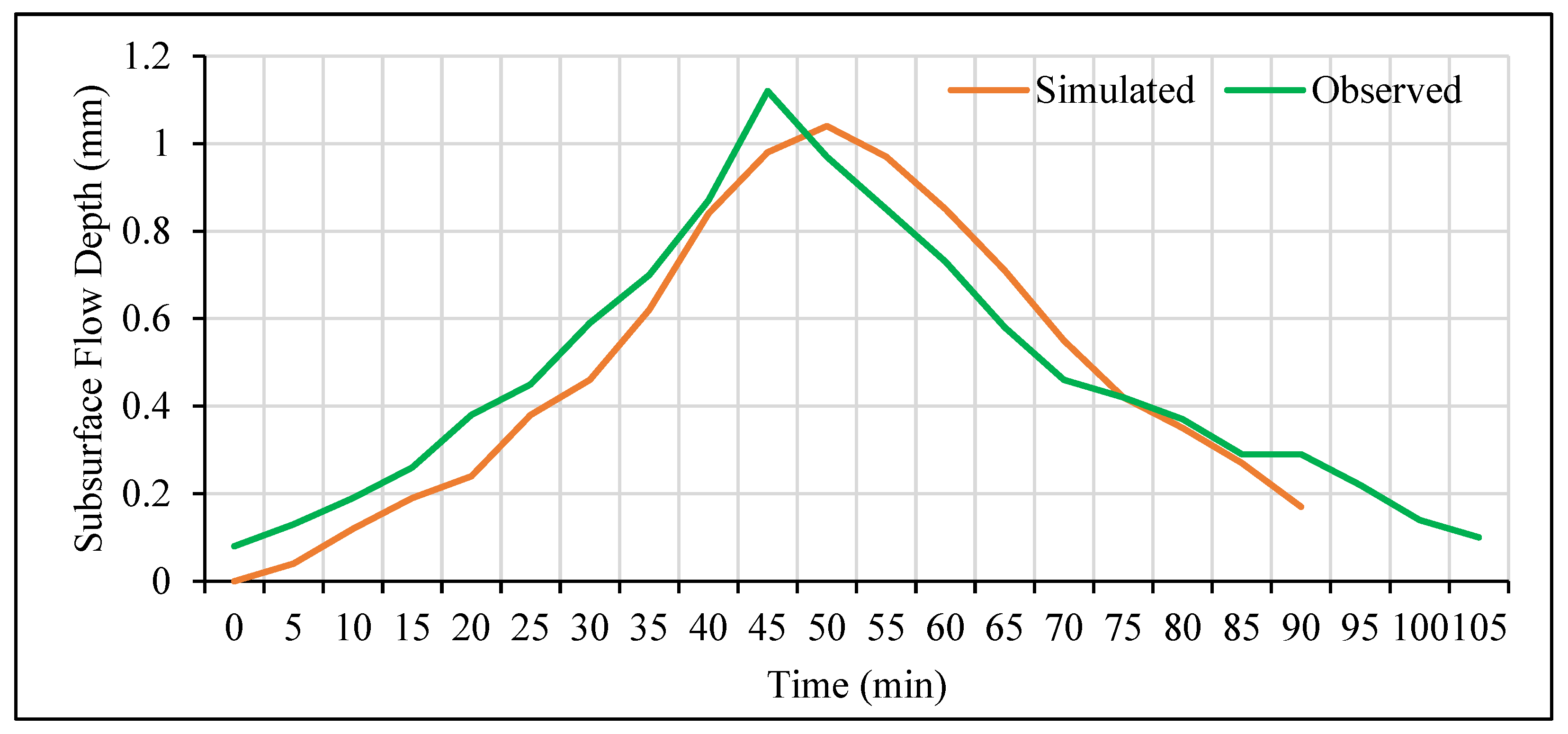
4.1.3. Subsurface Flow Observation

The channel constructed at the downslope of the hillslope plot for collecting runoff was provided with holes on the side of the plot to collect the subsurface flow. The experiment for subsurface flow observation was carried out in a vegetated condition. From the experiment it was evident that in vegetated conditions due to presence of macropores, subsurface flow played an active part in the channel flow. Although the subsurface flow started late, it lasted for a longer time even after the rainfall experiment has stopped. Figure 9 shows the observed subsurface flow recorded during and after the rainfall simulation for a vegetated condition.

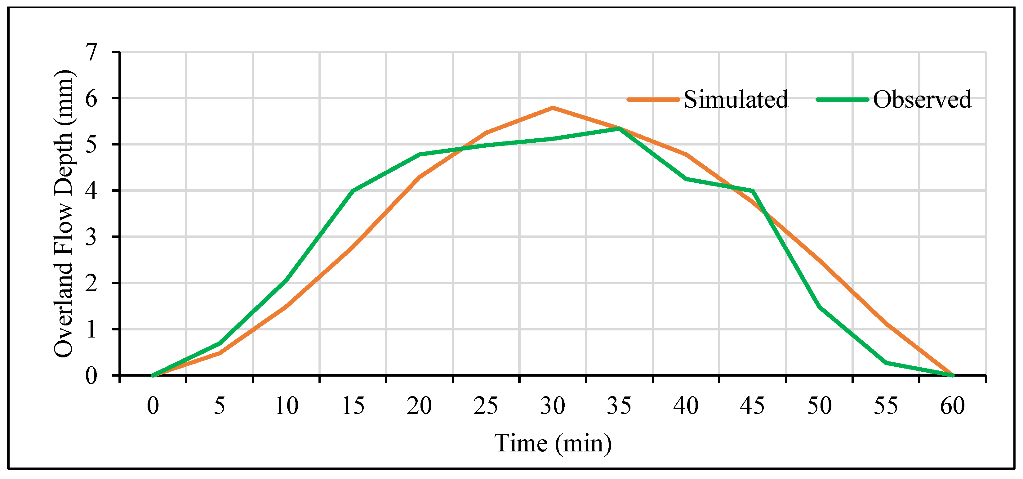
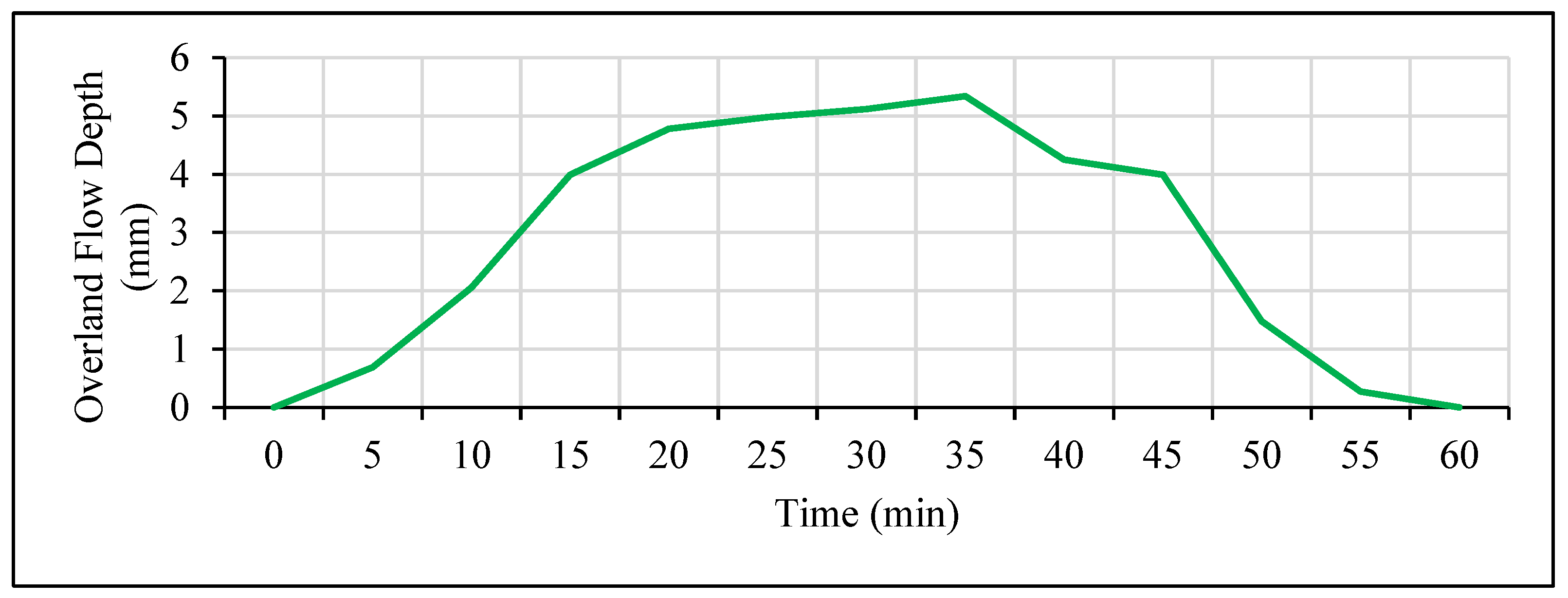
4.1.4. Overland Flow Observation

The water collected in the collecting channel flows to the stilling basin constructed at downslope of the hillslope plot. The water in the tank is measured at every 5-min interval using the digital water level recorder. Figure 10 shows the temporal variation of overland flow depth during and after the rainfall simulation experiment. It is observed from the figure that the peak overland flow occurs after around 8 min from the end of rainfall event.

4.2. Hydrological Modeling Results

This section shows the results of the rainfall simulator hillslope experiment. A comparison between the observed data of the hillslope rainfall simulator experiment and the results of the hydrological model was performed. The comparison is based on the obtained data of the rainfall–runoff relationship and soil moisture content.

Rainfall simulation experiments were performed for 100 mm/h rainfall intensity and field observations were taken for overland flow discharge and subsurface flow discharge. The hillslope hydrological model was run for the rainfall intensity 100 mm/h. The comparison of the observed and simulated overland flow hydrograph was done using the statistical parameter known as Nash–Sutcliffe model efficiency coefficient (E) [39]. The formula for the computation of Nash-Sutcliffe model efficiency is:

$$E=1-\left[\frac{\sum {(Q_o-Q_s)}^2}{\sum {(Q_o-{\overline{Q}}_o)}^2}\right]$$

(18)

where, ${\overline{Q}}_o$ is the mean of observed discharges, and $Q_s$ is modeled discharge. $Q_o$ is observed discharge at time t.

Nash–Sutcliffe efficiency can range from −∞ to 1. An efficiency of 1 (E = 1) corresponds to a perfect match of modeled discharge to the observed data. An efficiency of 0 (E = 0) indicates that the model predictions are as accurate as the mean of the observed data, whereas an efficiency less than zero (E < 0) occurs when the observed mean is a better predictor than the model or, in other words, when the residual variance (described by the numerator in the expression above), is larger than the data variance (described by the denominator). Essentially, the closer the model efficiency is to 1, the more accurate the model is.

For comparison of observed and simulated overland flow hydrograph (Figure 11 and Figure 12), correlation coefficient (R²) and Nash–Sutcliffe efficiency coefficient were computed. The coefficients were found to be R² = 0.95 and E = 0.91, which is quite satisfactory.

The developed conceptual hillslope hydrological model results also include components of macropore storage i.e., lateral infiltration into unsaturated matrix (Q_lu), lateral exfiltration out of saturated soil matrix (q_ls), and lateral exfiltration out of soil matrix as interflow (Q_li). As the rainfall starts, water enters into the macropore by directly falling into it or through overland flow (runoff). The infiltrated water initially enters the main bypass (MB) domain and the internal catchment (IC) domain. The macropores in the MB domain are well connected throughout the depth of the soil while IC domain ends at different depths with no connection between them. After rainfall initiation, the soil gets saturated and swells. As the rainfall continues, the water pressure starts building up on the saturated macropores because of which water fraction already present in the macropores starts moving laterally into the groundwater (Q_ls). After the rainfall, the Q_ls component starts decreasing with a decrease in water pressure on the macropores. In contrast, Q_lu increases with time as water moves laterally to the unsaturated zone from the macropore domain. This occurs where the stored macropore water is in contact with unsaturated soil matrix. The lateral infiltration occurs due to absorption of macropore water because of capillary force. As the soil gets saturated, the water starts flowing out of it into the macropores, which is termed as Q_li. This is the special case of exfiltration. The hillslope hydrological model results for macropore storage components for rainfall intensities of 100 mm/h are shown in Figure 13.

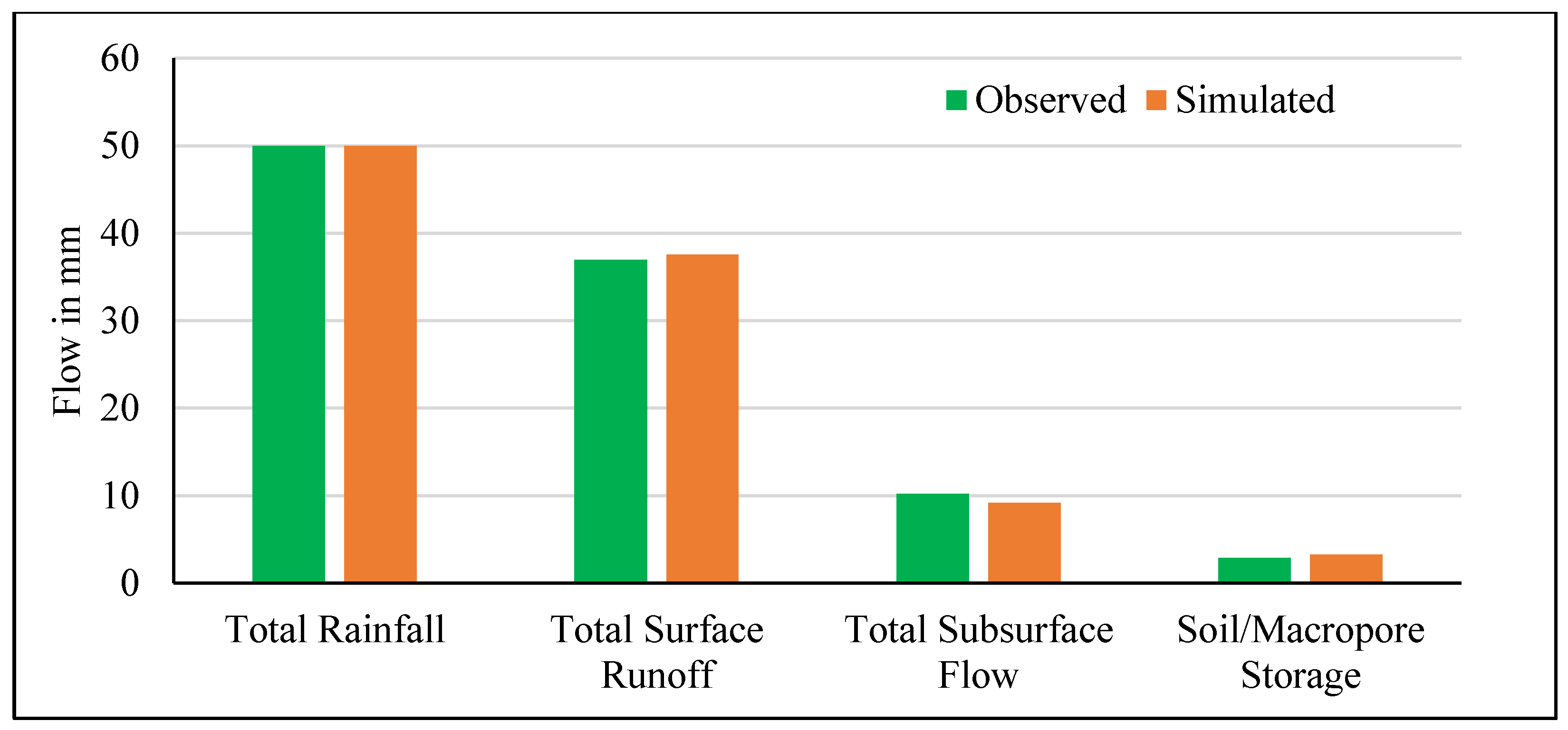
4.3. Water Balance Analysis

The water stored in the soil column (soil moisture) is very dynamic in space and time, however, in an event-based rainfall-runoff experiment, quantification of water absorbed/stored by the soil is essential. Traditionally, the accuracy of hydrological models is only tested by comparing model predicted runoff/discharge against the observed runoff/discharge. However, in the present case the developed hillslope hydrological model not only estimates surface and subsurface runoff but also quantifies the macropore storage in the study area. As such, an attempt has been made in the present study to validate the macropore storage results of developed model by using water balance approach. The water balance has been solved using observed components of the short term (temporal) water balance equation. The residual in the observed water balance excursive was assumed as water stored in the macropore/soil column. Thus, estimated soil water storage is used to validate the macropore storage predicted by the model. The results of water balance are shown in Figure 14. The model overpredicted the soil/macropore storage component by 0.38 mm, which is 13% of the observed residual water content. It was observed from the experimental results that around 20% of the total runoff comes in the form of subsurface flow. This higher fraction of subsurface contribution in total runoff is mainly due to the macropore-dominated flow pathways present in the soil column of the study plot.

5. Summary and Conclusions

This study delivers a useful description of a hillslope rainfall simulator experiment to estimate the hydrological response to high intensity rainfall over a hillslope plot size of 50 m². The rainfall simulator was designed to reflect the physical characteristics of natural rainfall event in terms of raindrop size, intensity, uniformity, continuity and kinetic energy. The rainfall simulator allowed us to vary rainfall intensity and duration with the help of nozzle pressure and control valves. The rainfall event was simulated for 100 mm/h intensity for 30 min. The surface runoff, subsurface runoff response and soil moisture were monitored throughout the experiment. The soil moisture profile observed during and after the rainfall simulation experiment revealed that soil moisture plays an important role in the runoff generation process only during inception phase. After some time, soil moisture remained constant mostly in bottom soil layer at a depth of 600–1000 mm. The runoff and macropore storage components were also estimated through a hillslope hydrological model. To calibrate the model, several field investigations were carried out to estimate the vertical profile of soil macropore fraction, moisture variability and soil characteristics. The observed and simulated water balance components were then compared by Nash–Sutcliffe model efficiency coefficient and found a satisfactory match between them. The correlation coefficient and Nash model efficiency were computed as 0.95 and 0.91, respectively, for surface runoff. The model accuracies in predicting surface runoff, subsurface runoff and soil/macropore storage were 98%, 90% and 86%, respectively.

This study showed that the influence of soil and macropore characteristics on drainage for the hillslope experimental conditions depends largely on the soil characteristics. It was also found that subsurface flow plays important role in generation of surface runoff in hilly watersheds. Therefore, based on our results, advances can be made for future experiments to quantify subsurface storm flow, saturation excess flow, overland flow, return flow and pipe storage processes under varying topography, vegetative cover, and rainfall intensities. In conclusion, this study is good food for thought for hydrologists and soil scientists with respect to future experiments.

References

1. Band, L.E.; Patterson, P.; Nemani, R.; Running, S.W. Forest ecosystem processes at the watershed scale: Incorporating hillslope hydrology. Agric. For. Meteorol. 1993, 63, 93–126. [Google Scholar] [CrossRef]
2. Nolan, S.C.; van Vliet, L.J.P.; Goddard, T.W.; Flesch, T.K. Estimating storm erosion with a rainfall simulator. Can. J. Soil Sci. 1997, 77, 669–676. [Google Scholar] [CrossRef]
3. Beven, K.J.; Germann, P.J. Macropores and water flow in soils. Water Resour. Res. 1982, 18, 1311–1325. [Google Scholar] [CrossRef]
4. Shougrakpam, S.; Sarkar, R.; Dutta, S. An experimental investigation to characterize soil macroporosity under different land use and land covers of northeast India. J. Earth Syst. Sci. 2010, 119, 655–674. [Google Scholar] [CrossRef]
5. Yvonne, S.; Martine, J.; Ploeg, V.D.; Teuling, A.J. Rainfall Simulator Experiments to Investigate Macropore Impacts on Hillslope Hydrological Response. Hydrology 2016, 3, 39. [Google Scholar]
6. Adams, R.; Parkin, G.; Rutherford, J.C.; Ibbitt, R.P.; Elliott, A.H. Using a rainfall simulator and a physically based hydrological model to investigate runoff processes in a hillslope. Hydrol. Process. 2005, 19, 2209–2223. [Google Scholar] [CrossRef]
7. Sheridan, G.J.; Noske, P.; Lane, P.; Sherwin, C. Using rainfall simulation and site measurements to predict annual interrill erodibility and phosphorus generation rates from unsealed forest roads: Validation against in-situ erosion measurements. CATENA 2008, 73, 49–62. [Google Scholar] [CrossRef]
8. Arnaez, J.; Lasanta, T.; Ruiz-Flaño, P.; Ortigosa, L. Factors affecting runoff and erosion under simulated rainfall in Mediterranean vineyards. Soil Tillage Res. 2007, 93, 324–334. [Google Scholar] [CrossRef]
9. Verbist, K.; Cornelis, W.M.; Gabriels, D.; Alaerts, K.; Soto, G. Using an inverse modelling approach to evaluate the water retention in a simple water harvesting technique. Hydrol. Earth Syst. Sci. 2009, 13, 1979–1992. [Google Scholar] [CrossRef]
10. Humphry, J.B.; Daniel, T.C.; Edwards, R.D.; Sharpley, A.N. A portable rainfall simulator for plot scale runoff studies. Appl. Eng. Agric. 2002, 18, 199–204. [Google Scholar] [CrossRef]
11. Sousa Júnior, S.F.; Siqueira, E.Q. Development and Calibration of a Rainfall Simulator for Urban Hydrology Research. In Proceedings of the 12th Intenational Conference on Urban Drainage, Porto/Alegre, Brazil, 11–16 September 2011.
12. Pe’ rez-Latorre, F.J.; Castro, L.; Delgado, A. A comparison of two variable intensity rainfall simulators for runoff studies. Soil Tillage Res. 2010, 107, 11–16. [Google Scholar] [CrossRef]
13. Abudi, I.; Carmi, G.; Berliner, P. Rainfall simulator for field runoff studies. J. Hydrol. 2012, 454–455, 76–81. [Google Scholar] [CrossRef]
14. Bubenzer, G.D. Inventory of rainfall simulators. In Proceedings of the Workshop on Rainfall Simulators; Agricultural Research, Science and Education Agency, USDA: Washington, DC, USA, 1979; pp. 120–130. [Google Scholar]
15. Meyer, L.D.; McCune, D.L. Rainfall simulator for runoff plots. Agric. Eng. 1958, 39, 644–648. [Google Scholar]
16. Swanson, N.P. Rotating–boom rainfall simulator. Trans. ASAE 1965, 8, 71–72. [Google Scholar] [CrossRef]
17. Foster, G.R.; Neibling, W.H.; Natterman, R.A. A Programmable Rainfall Simulator; American Society Agricultural Engineers: St. Joseph, MI, USA, 1982. [Google Scholar]
18. Moore, I.D.; Hirschi, M.C.; Barfield, B.J. Kentucky rainfall simulator. Trans. ASAE 1983, 26, 1085–1089. [Google Scholar] [CrossRef]
19. Shelton, C.H.; von Bernuth, R.D.; Rajbhandari, S.P. A continuous–application rainfall simulator. Trans. ASAE 1985, 28, 1115–1119. [Google Scholar] [CrossRef]
20. Miller, W.P. A solenoid–operated, variable intensity rainfall simulator. Soil Sci. Soc. Am. J. 1987, 51, 832–834. [Google Scholar] [CrossRef]
21. Meyer, L.D. Simulator of rainfall for soil erosion research. Trans. ASAE 1965, 8, 63–65. [Google Scholar] [CrossRef]
22. Moore, I.D. Effect of surface sealing on infiltration. Trans. ASAE 1981, 24, 1547–1552. [Google Scholar] [CrossRef]
23. Kathiravelu, G.; Lucke, T.; Nichols, P. Rain drop measurement techniques: A review. Water 2016, 8. [Google Scholar] [CrossRef]
24. Hudson, N.W. The Influence of Rainfall on the Mechanics of Soil Erosion with Particular Reference to Southern Rhodesia, Unpub. Master’s Thesis, University of Cape Town, Cape Town, South Africa, 1965. [Google Scholar]
25. Kara, T.; Ekmekci, E.; Apan, M. Determining the Uniformity Coefficient and Water Distribution Characteristics of Some Sprinklers. Pak. J. Biol. Sci. 2008, 11, 214–219. [Google Scholar] [CrossRef] [PubMed]
26. Grierson, I.T.; Oades, J.M. A rainfall simulator for field studies of rainfall and runoff. J. Agric. Res. 1977, 22, 37–44. [Google Scholar]
27. Wischmeier, W.H.; Smith, D.D. Rainfall energy and its relation to soil loss. Trans. Am. Geophys. Union 1958, 39, 285–291. [Google Scholar] [CrossRef]
28. Lows, J.O.; Parson, D.A. The relationship of raindrop size to intensity. Trans. Am. Geophys. Union 1943, 24, 452–460. [Google Scholar] [CrossRef]
29. Weiler, M.; Flühler, H. Inferring flow types from dye patterns in macroporous soils. Geoderma 2004, 120, 137–153. [Google Scholar] [CrossRef]
30. Dutta, S.; Zade, M. RISE-A Distributed Hydrologic Model for Rice Agriculture: Concept and Evaluation. In Watershed Hydrology; Singh, V.P., Yadava, R.N., Eds.; Allied Publisher: New Delhi, India, 2003; pp. 240–251. [Google Scholar]
31. Agnese, A.; Baiamonte, G.; Corrao, C. A simple model of hillslope response for overland flow generation. Hydrol. Process. 2001, 15, 3225–3238. [Google Scholar] [CrossRef]
32. Anderson, S.P.; Dietrich, W.E.; Montgomery, D.R.; Torres, R.; Conrad, M.E.; Loague, K. Subsurface flow paths in a steep unchanneled catchment. Water Resour. Res. 1997, 33, 2637–2653. [Google Scholar] [CrossRef]
33. Horton, R.E. The role of infiltration in the hydrological cycle. Trans. Am. Geophys. Union 1933, 14, 446–460. [Google Scholar] [CrossRef]
34. Freeze, R.A. Role of subsurface flow in generating surface runoff. 2. Upstream source areas. Water Resour. Res. 1972, 8, 1273–1283. [Google Scholar] [CrossRef]
35. Dunne, T. Field studies of hillslope processes. In Hillslope Hydrology; Kirkby, M.J., Ed.; McGraw-Hill: New York, NY, USA, 1978; pp. 227–293. [Google Scholar]
36. Kroes, J.G.; van Dam, J.C.; Groenendijk, P.; Hendriks, R.F.A.; Jacobs, C.M.J. SWAP Version 3.2. Theory Description and User Manual; Alterra Report 1649; Alterra: Wageningen, The Netherlands, 1964. [Google Scholar]
37. Shakya, N.M.; Chander, S. Modelling of hillslope runoff processes. Environ. Geol. 1998, 35, 115. [Google Scholar] [CrossRef]
38. Knasiak, K.; Schick, R.J.; Kalata, W. Multiscale Design of Rain Simulator. In Proceedings of the 20th Annual Conference on Liquid Atomization and Spray Systems, Chicago, IL, USA, 15–18 May 2007.
39. Nash, J.E.; Sutcliffe, J.V. River flow forecasting through conceptual models part I—A discussion of principles. J. Hydrol. 1970, 10, 282–290. [Google Scholar] [CrossRef]
Figure 1. (a) Location of the study area; (b) Experimental hillslope plot setup.
Hydrology 04 00017 g001
Figure 2. (a) Schematic diagram of the experimental setup; (b) Digital elevation model (DEM) of the experimental hillslope plot. DWLR: Digital water level recorder.
Hydrology 04 00017 g002
Figure 3. (a) Raindrop flour pellet after oven drying; (b) Measurement of the raindrop size by flour pellet method.
Hydrology 04 00017 g003
Figure 4. Rainfall experiment for calculation of coefficient of uniformity.
Hydrology 04 00017 g004
Figure 5. (ak) Subset digitally pre-processed images of soil samples used in macropore analysis of the hillslope at different depths mentioned in the figure.
Hydrology 04 00017 g005
Figure 6. Conceptual flow chart of the hillslope hydrological model. M.C.: Moisture content, F.C.: Field capacity.
Hydrology 04 00017 g006
Figure 7. (ad) Soil moisture variations at experimental hillslope plot.
Hydrology 04 00017 g007
Figure 8. Depth-wise dye coverage distribution in the soil column.
Hydrology 04 00017 g008
Figure 9. Subsurface flow for rainfall intensity of 100 mm/h for 30 min.
Hydrology 04 00017 g009
Figure 10. Overland flow hydrograph for rainfall intensity of 100 mm/h for 30 min.
Hydrology 04 00017 g010
Figure 11. Subsurface flow hydrograph for rainfall intensity of 100 mm/h for 30 min.
Hydrology 04 00017 g011
Figure 12. Overland flow hydrograph for rainfall intensity of 100 mm/h for 30 min.
Hydrology 04 00017 g012
Figure 13. Change in macropore storage with respect to time for 100 mm/h rainfall intensity. Soil matrix; Qli: lateral exfiltration out of the saturated soil matrix by interflow out of a zone with perched groundwater; Qls: lateral exfiltration out of the saturated soil matrix; Qlu: lateral infiltration into the unsaturated soil matrix.
Hydrology 04 00017 g013
Figure 14. Water balance for rainfall intensity of 100 mm/h for 30 min.
Hydrology 04 00017 g014