
Trends and Changes in Recent and Future Penman-Monteith Potential Evapotranspiration in Benin (West Africa)

1
Laboratory of Applied Hydrology, University of Abomey-Calavi (UAC), Cotonou 01 BP 4521, Benin
2
West African Science Service Center on Climate Change and Adapted Land Use (WASCAL), GRP Climate Change and Water Resources, University of Abomey-Calavi (UAC), Abomey-Calavi BP 2008, Benin
*
Author to whom correspondence should be addressed.
Hydrology 2017, 4(3), 38; https://doi.org/10.3390/hydrology4030038
Submission received: 28 June 2017
/
Revised: 27 July 2017
/
Accepted: 28 July 2017
/
Published: 3 August 2017
Abstract
:In this study, the recent variability of the annual potential evapotranspiration (PET) of six synoptic stations of Benin was carried out. The future changes of PET under RCP4.5 and RCP8.5 scenarios were also quantified under three different projected periods (P1 = 2011–2040, P2 = 2041–2070 and P3 = 2071–2100) compared to the reference period (1981–2010). The results show a high variability of PET at all stations over the baseline period with alternating of deficit and excess periods. The Representative Concentration Pathways (RCP4.5 and RCP8.5) scenarios indicate that annual PET gradually increase and reach its maximum on 2100. However, PET’s changes from the two forcing scenarios start to diverge only around 2070 and this divergence is maximal on 2100. The rates of changes related to the baseline period vary from 2 to 7% for P1 and both scenarios, 5 to 10% for P2 and both scenarios, 7 to 12% for P3 and RCP4.5 scenario and 15 to 20% for P3 and RCP8.5 scenario. At seasonal scale, the results show a progressive increase (from 15 to 25% related to the baseline period) of PET until 2100 for January, February, June, July and December. In April, May, August, September and October, there is a slight decrease (from −5 to 0%) of PET according to RCP4.5 scenario while there is a slight increase (0 to 5%) for RCP8.5 scenario.
1. Introduction
Evapotranspiration, including evaporation and transpiration, plays a crucial role in the heat and mass fluxes of global and regional atmospheric systems. Understanding the mechanism of evapotranspiration is vital in hydrological and agricultural studies at the global, regional and local scales [1,2,3,4,5]. Evapotranspiration estimates are a required input for hydrological modeling, alongside rainfall. Evapotranspiration changes, on their own or in combination with rainfall changes, can contribute to changes in hydrological indices such as mean monthly river flows. Evapotranspiration is evaluated through potential evapotranspiration (PET), which represents the maximum evaporative demand on a reference grass crop under climatic conditions where water availability is not a limiting factor [6]. Many studies have investigated the spatiotemporal variability of PET in different regions [2,5,7,8,9,10,11,12,13,14,15,16] and most of them lead to changes in evapotranspiration, certainly due to the warming of the earth. According to [17,18,19], climate change due to human activity will have a negative impact on the hydrological cycle and on water resources. In particular, global warming will lead to a possible intensification of the hydrological cycle resulting from increase of precipitations and PET [20,21,22]. Recent studies on the trend analysis of the PET show mixed results. Indeed, upward trends were detected in the long-term series of PET in England [23,24], on the Nile Basin [25], in Burkina Faso [26], in India [27], while downward trends were found in India [28], in Italy [29], in the Tibetan Plateau [30], in China [31], etc.
Many formulas have been developed to estimate PET. Ref. [32] have classified these formulas into three main categories according to the climatic parameters they take into account: mass transfer based formulas, radiation based formulas and temperature based formulas. The Penman-Monteith formula [6], which takes into account all the climatic parameters of these three categories, is considered to be the reference formula for the estimation of PET [32,33,34,35,36,37].
In the last decades, many studies on the variability of PET and the impacts of climate change on PET were carried out. However, in West Africa, very few studies were focused on the spatial and temporal variability of PET. The impacts of climate change on the PET at short, medium and long term are not explored in West Africa. This paper aims to analyze the recent and future variability of PET in Benin country, taking into account the changes in many climatic parameters (speed Wind, radiation, air humidity, temperature) for hydrological forecasts.
2. Study Area, Data and Methods
2.1. Study Area and Data
Covering an area of 112,622 km2 and located in West Africa, Benin country consists of a narrow band of land oriented perpendicularly to the coast of the Gulf of Guinea [38]. It is bounded in the North by Burkina Faso and Niger Republics, in the South by the Atlantic Ocean, in the East by the Federal Republic of Nigeria and in the West by the Republic of Togo. With a coastline of 124 km, it extends from north to south over a length of 672 km and reaches a width of 324 km at its widest point [38] (Figure 1).
The data used in this study are of two types: observed data and simulated data from Regional Climate Models (RCMs). A historical dataset from 1967 to 2010, composed of data from 6 meteorological stations (Table 1), was provided by the Benin Meteorological Agency. Daily maximum temperature (Tmax, °C), daily minimum temperature (Tmin, °C), daily maximum humidity (RHmax, %), daily minimum humidity (RHmin, %), wind speed (WS, m·s−1) observed at 2 m height, and daily sunshine duration (SD, h) data were available.
The 0.5 ° × 0.5 ° gridded data of West Africa from 1951 to 2100 simulated by three RCMs (SMHI-RCA4, MPI-REMO, DMI-HIRHAM5) of historical simulation and under the Representative Concentration Pathways (RCPs) climatic scenarios were obtained from CORDEX Africa project. The RCPs scenarios are using because they were developed from sets of existing scenarios. The RCPs scenarios include four major families: the RCP2.6 scenarios, which represents the radiative forcing trajectory that reaches a peak of 3 W/m2 before 2100 and drops to 2.6 W/m2 in 2100 [39]; the RCP4.5 which describes stabilization without exceeding 4.5 W/m2 after 2100 [40]; the RCP6 which is similar to RCP4.5, with stabilization at 6 W/m2 after 2100 [41] and the RCP8.5, which corresponds to the profile of the growing radiative forcing leading to 8.5 W/m2 in 2100 [42]. West Africa is a developing region which would need to use more and more energy than what is using now then the RCP2.6 scenario with a low level of greenhouse gas emissions is not suitable for climate prediction in this region. The RCP6 scenario is similar to the RCP4.5 scenario; it is not often taken into account in climate projections. The scenarios RCP4.5 and RCP8.5 are considered in this study. These data included daily average temperature (Ta, °C), Tmax, Tmin, daily wind speed, daily RHmax, RHmin and daily net radiation (RS, MJ·m−2·day−1). The characteristics of used RCMs are shown in Table 2.
2.2. Methods
2.2.1. PET computing
The Penman-Monteith formula was proposed by the Food and Agriculture Organization of the United Nations (FAO) for estimating the water requirements of plants on irrigation schemes. The used formula to compute PET is the FAO Penman-Monteith Equation (1) presented by [6].
PET: potential evapotranspiration (mm·day−1), Rn: net radiation at the crop surface (MJ·m−2·day−1), G: soil heat flux density (MJ·m−2·day−1), T: daily mean air temperature at 2 m height (°C), u2: wind speed at 2 m height (m·s−1), es: saturation vapor pressure (kPa), ea: actual vapor pressure (kPa), es − ea: saturation vapor pressure deficit (kPa), Δ: slope vapor pressure curve (kPa·°C−1), γ: psychrometric constant (0.066) (kPa·°C−1).
(°C) is daily mean air temperature.
Tr Temperature at dew point (°C).
Rn = Rns − Rnl with Rns = (1 − α)·Rs and Rnl = RLWe − RLWr where Rs = downward shortwave radiation, α = albedo, RLWe = upward longwave radiation, RLWr = downward longwave radiation.
2.2.2. PET Inter-Annual Variability Assessment
We used the Lamb Index to analyze the inter-annual variability of recent PET. The Lamb Index determines the nature excess, normal or deficit of a given year according to the study period. This index IPET is defined as follows by Equation (5)
where PETi stands for the value of the annual PET of the year i; PETm, the mean of PET over the study period, and , the standard deviation of the data.
2.2.3. Mann-Kendall Test
The Mann-Kendall test has been widely used to test for randomness in hydrology and climatology [46,47,48,49]. It is calculated via the following equation:
where n is the number of data points, xi and xj are the ith and jth data values in the time series (j > i), respectively, and sgn(xj − xi) is the sign function determined as:
In cases when the sample size n > 10, the mean value (µ(S)) and variance (σ2(S)) are given by the following equation:
where m is the number of tied groups and ti is the number of ties of extent i. A tied group is a set of sample data with the same value. In the absence of ties between the observations, the variance is calculated by the following equation:
The standard normal test statistic ZS is calculated as:
A positive ZS value indicates increasing trends; otherwise it represents decreasing trends. At the 5% significance level, the null hypothesis of the presence of no trend is rejected if |ZS| > 1.96.
2.2.4. Bias Correction
There is a large number of downscaling methods. Two (2) of the most widely used methods for bias correction are used in this paper. These methods are: ‘Scaling’ and ‘Empirical Quantile Mapping’ (EQM). The Scaling method aims to perfectly match the monthly mean of corrected values with that of observed ones [50,51]. It operates with monthly correction values based on the differences between observed and raw data (raw RCM simulated data in this case). PET as well as temperature is generally corrected with an additive term on a monthly basis:
where PETc,m,d is corrected PET on the dth day of mth month, and PETRCM,m,d is the raw PET on the dth day of mth month. Δo,m and ΔRCM,m are respectively the mean values of observed and simulated PET of the month m.
The Quantiles-Quantiles methods consist in correcting the quantile values of the model by those calculated from the observations. At each point of the model, for each meteorological variable, the 99 percentiles of the daily series are calculated. The 99 percentiles of the observed series are also calculated. Each variable is corrected independently and at the daily time step. The correction function consists in associating each percentile of the model with the observed percentile. The EQM method uses empirical distribution functions [52,53,54]. This method should produce the best correction, but depends on many degrees of freedom and cannot be stationary and therefore may transgress this assumption in future periods. However, for applications on climate change, it is assumed that the transfer function remains constant over time [55], which is a trivial hypothesis [56]. The EQM method is constructed by calculating the empirical Probability Distribution (PDF) functions but uses the Cumulative Distribution Functions (CDF) for the correction:
where y is the corrected meteorological parameter and x its simulated value by the model ; FRCM is the CDF of simulated data by the RCM and Fobs−1 is the inverse of the CDF of the observed data.
The performance of each bias correction method is evaluated using the Root-Mean-Square Error (RMSE) and the Mean Absolute Error (MAE).
- The Root-Mean-Square Error (RMSE)
The Root-Mean-Square Error between two series is the distance between the means of these two series. The RMSE is particularly close to zero as the two series are similar.
- The Mean Absolute Error (MAE)
The MAE of two series is the mean of absolute values of error between the data of the two series taken in pairs. Like the RMSE, it is even closer to zero as the two series considered are similar.
2.2.5. Changes Rates
The rates of changes were calculated by considering four (04) different periods. The first period is the baseline period (1981–2010). The three other periods are the projected periods (2011–2040 (P1), 2041–2070 (P2) and 2071–2100 (P3)). For each period, the mean was calculated and then the rate of changes was calculated using Equation (15).
where is the mean of PET over the considered projected period, and is the mean of PET over the reference period.
3. Results and Discussion
3.1. Recent Inter-Annual Variability of PET
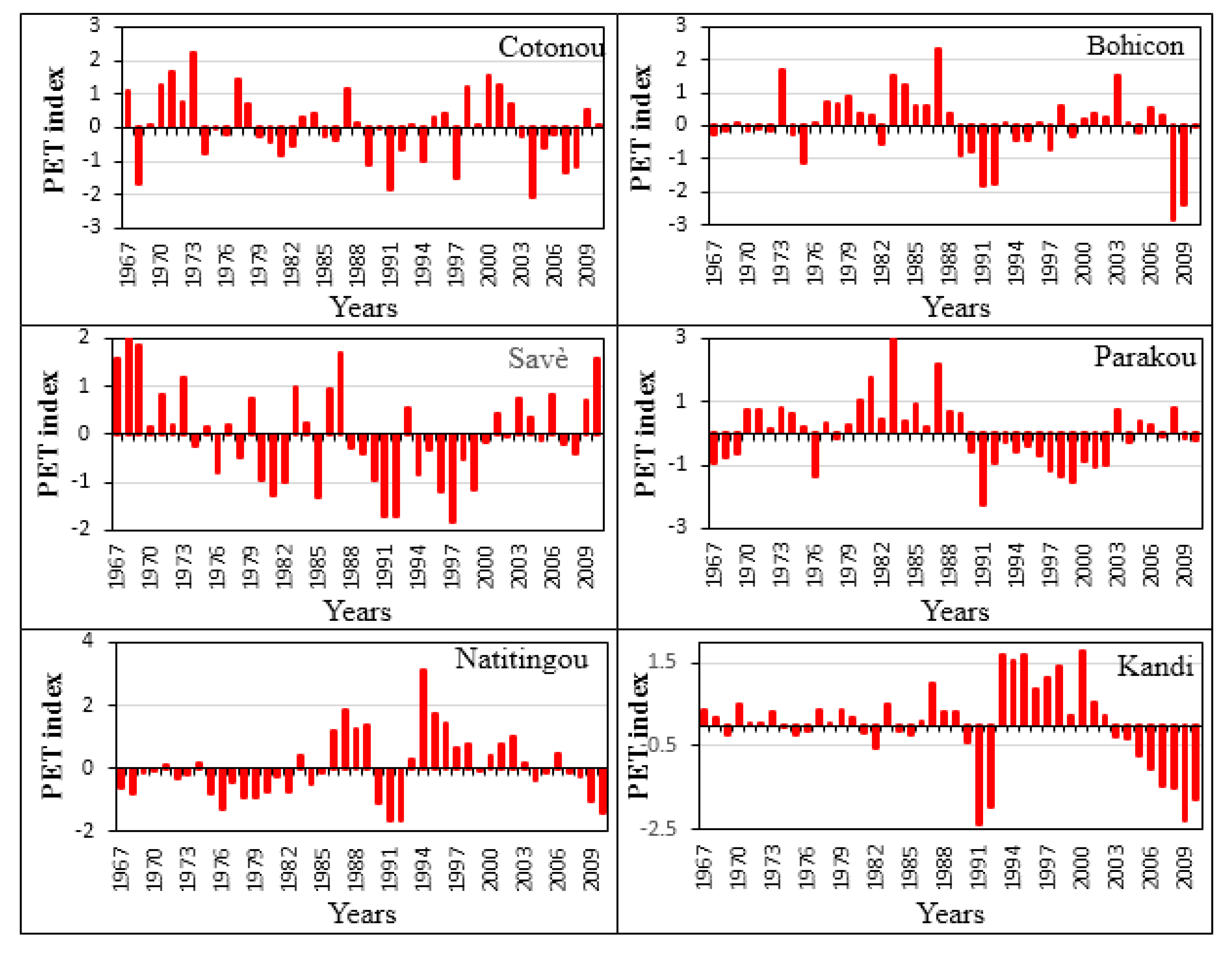
Over the period from 1967 to 2010, annual PET varies from one station to another and are characterized by high variability. There are frequent alternations between periods of PET excess and periods of PET deficit (Figure 2). At Cotonou, the period from 1967 to 1979 is a period of PET excess with a few deficit years. This period is followed by a deficit period (1980 to 1997) with some excess years. The period from 1998 to 2010 is characterized by an alternation between a short excess period (1998–2002) and a short deficit period (2003–2008). Bohicon station is characterized by a short period (1967–1973) of low PET variability. This period is followed by a long period (1974–1988) of excess of PET. The period from 1989 to 1997 is a deficit period while the period from 1998 to 2008 is an excess period. At Savè station, the periods from 1967 to 1973 and from 2001 to 2010 were excess in PET whereas the period from 1974 to 2000 was a deficit period with a few years of PET surpluses. At Parakou, the periods from 1967 to 1969 and from 1990 to 2002 are periods of deficit of PET while the periods from 1970 to 1989 and from 2003 to 2010 are periods of PET excess with a few deficit years. At Natitingou, the periods from 1967 to 1985, from 1990 to 1992 and from 2004 to 2010 are periods of PET deficit while the other periods are periods of excess. At Kandi, the period from 1967 to 1986 is a period of low variability of PET. After this period, short periods of PET excess (1987–1999 and 1993–2002) and short periods of PET deficit (1990–1992 and 2003–2010) were alternated.
3.2. PET Trends Analysis
The results showing trends in monthly and annual PET for the period of 1981–2010 are presented in Table 3. At Cotonou, 7 months (January, March to June, October and November) indicate decreasing trends PET while the other months show increasing trends. Annual PET shows decreasing trend. Only April trend (Zs = −2.14) and December trend (Zs = +3.00) are statistically significant at 95% level. At Bohicon, July and December months show increasing trends while other months and annual PET indicate decreasing trends. June trend (Zs = −2.18) and December trend (Zs = +2.32) are statistically significant at 95% level. Few months show insignificant decreasing trend at Savè station. These months are January, April, May and August. The other months and annual PET indicate increasing trends with statistically significant at 95% level for July, October, November and December. At Parakou, July, November and December months indicate increasing trends of PET but these trends are not significant at 95% level. The other months and annual PET show decreasing trends that are statistically significant at 95% level for March, April and May. Natitingou station indicates only decreasing trends for all months and annual PET. The trends are all statistically insignificant at 95% level. At Kandi, it is only in December, PET shows increasing trend but this trend is statistically insignificant at 95% level. All other months and annual PET indicate decreasing trends with statistically significant at 95% level from May to September. The different trends obtained are consistent with the results of recent studies. Indeed, upward trends have been detected in England [23,24], on Nile Basin [25], in Burkina Faso [26], in India [27] while downward trends were detected in India [28], in Italy [29], in the Tibetan Plateau [30] and in China [31]. A global study finds large basins with positive (e.g., Niger), negative (e.g., Amazon) and non-significant (e.g., Congo) PET trends over 1958–2001 [57]. Both increasing and decreasing trends have been found in China [58,59].
3.3. Bias Correction Performances
Figure 3 shows annual PET estimated from the observed meteorology variables and those estimated from simulated variables by RCMs. The figure indicates that HIRHAM5 and RCA4 models overestimated annual PET at all stations. PET estimated by RCA4 model is higher than those of the HIRHAM5 model. REMO model underestimates annual PET at Cotonou and Bohicon but at the other stations, the estimated PET is more consistent with the observed PET. These results indicate that estimated PET from climate models contains biases that need to be corrected.
Table 4 shows the performances of bias correction methods in calibration and validation periods. In calibration, for HIRHAM5 model MAE values range from 0.91 to 1.34 for the uncorrected estimated PET while MAE values vary from 0.85 to 1.16 for the corrected PET with the Scaling method against 0.70 to 0.98 for those corrected by EQM method. In validation, MAE values range from 0.95 to 1.39 for uncorrected estimated PET, from 0.95 to 1.18 when the data are corrected with Scaling method and from 0.72 to 1.03 when the correction is made by using the EQM method. From this analysis it appears that EQM method is better compared to Scaling method for bias correction of estimated PET. For REMO model, in calibration, MAE values vary between 0.90 and 1.08 for uncorrected estimated PET while MAE values vary from 0.89 to 1.04 when the Scaling method is applied to correct the bias whereas MAE are of the order of 0.65 to 0.87 when the bias correction method is EQM. In validation, MAE values obtained with the uncorrected PET range from 0.89 to 1.12. After bias correction, MAE values remained unchanged with the Scaling method (0.89 to 1.10) while with the EQM method these values are between 0.66 and 0.92. As with HIRHAM5 model, EQM method is better than Scaling method at all synoptic stations in Benin. For RCA4 model, MAE values obtained with uncorrected PET vary from 0.96 to 1.44 in calibration and from 1.01 to 1.56 in validation. After bias correction with the Scaling method, MAE values range from 0.72 to 0.97 in calibration and 0.73 to 1.01 in validation, while for the EQM method MAE values are between 0.62 and 1.04 in calibration against 0.61 and 1.07 in validation. It is found that for RCA4 model, both methods perform well according to the stations. Indeed, at Cotonou and Kandi stations, the Scaling method presents good performances whereas at the other stations, EQM method is better than Scaling method.
RMSE values show almost identical results to those of MAE. In calibration for the three models, both bias correction methods and all stations, RMSE values are of the order of 0.0. In validation, they are between 0.0 and 0.3. From this analysis and from Figure 3 and Figure 4, it appears that bias correction methods reduce effectively RCMs biases. Here EQM method is better than Scaling method. This is why EQM method is chosen to bias correct projected PET under RCP4.5 and RCP8.5 scenarios of climate change.
3.4. Rates of Changes Related to the Baseline Period
3.4.1. Annual Changes
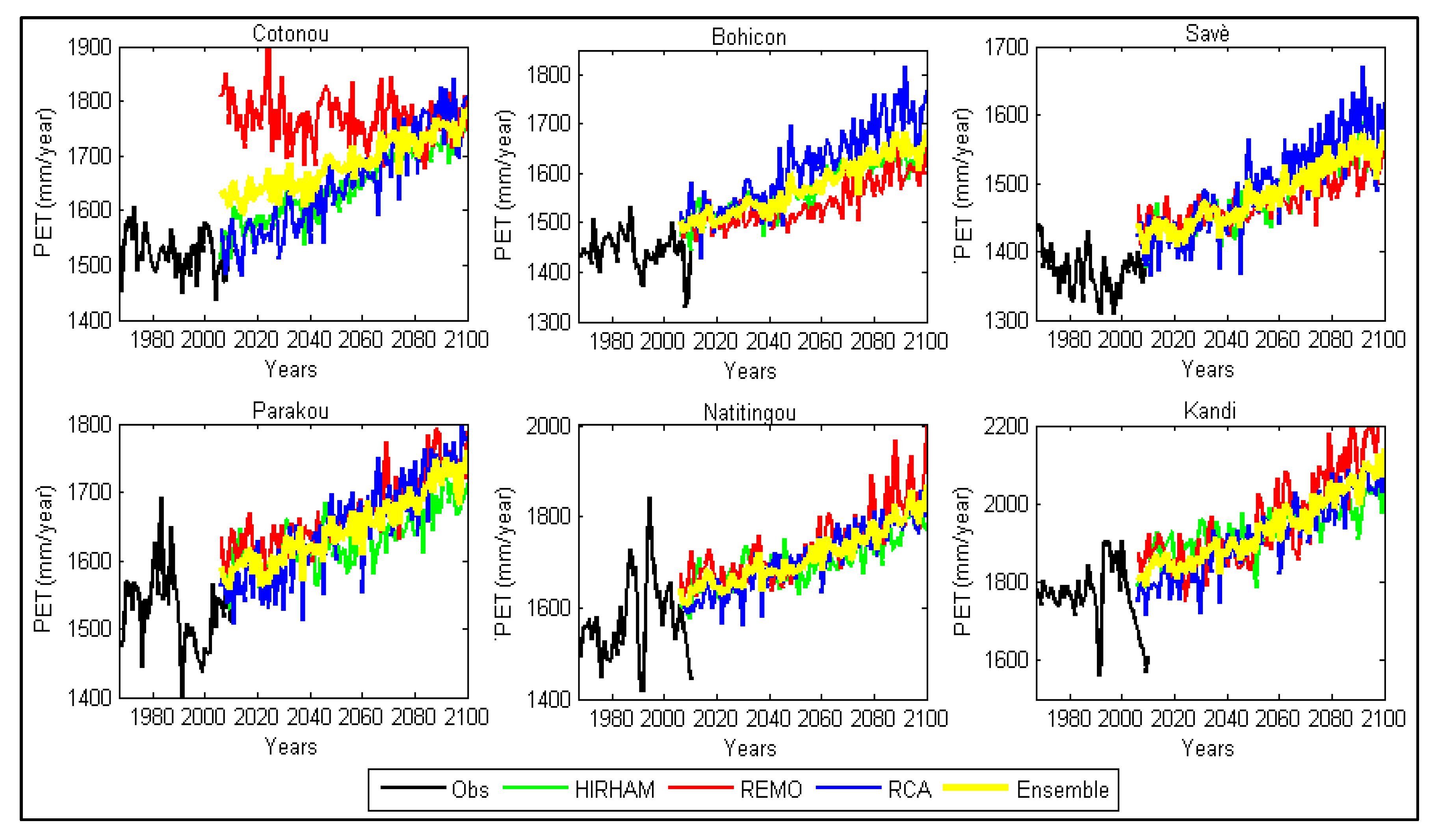
Figure 5 and Figure 6 show the evolution of annual PET from 1967 to 2100. Regardless of the climate change scenario and RCMs, projected PET indicates upward trends. According to the RCP4.5 scenario the increase will be continuous until 2070s then there is PET stabilization until 2100 while for the RCP8.5 scenario the increase will be continuous until 2100.
The changes induced by these continuous increases of annual PET are shown in Figure 7. During P1 period and under the RCP4.5 scenario, HIRHAM5 projects increases of 2.86 to 4.66% of annual PET compared to the baseline period. Over the same period, REMO model indicates increases of 4.81 to 5.58% except at Cotonou station with a rate of 1.11%. For RCA4 model, the rates of increase of PET are low and vary from 3.31 to 3.73 %, excepted Bohicon station where an increasing rate of 5.58% was found. The Ensemble of three models projects increases of 2.62 to 4.69%. According to the RCP8.5 scenario, models project increases of annual PET over P1 period that are slightly higher than those projected under the RCP4.5 scenario. Indeed, HIRHAM5 model projects increases of 4.44 to 7.25%, REMO model indicates increases of 4.28 to 7.17% except Cotonou station which projects a rate of increase of 16.02% compared to the baseline period. RCA4 model projects increases of 2.6 to 5.9%, while the Ensemble of three models projects increases of 4.99 to 7.69% related to reference period.
Over P2 period and under the RCP4.5 scenario, HIRHAM5 model projects increases of 5.03 to 7.71% of annual PET compared to the baseline period. REMO model predicts increases between 5.44% and 8.33%, with the exception of Cotonou station which indicates a very small decrease (−0.01%). RCA4 model forecasts increases of 6.26 to 8.76% while the Ensemble of these three models predicts increases of 4.13 to 7.64% of annual PET related to the reference period. According to the RCP8.5 scenario, the growth rates of PET over P2 period are higher than those obtained with the RCP4.5 scenario. The HIRHAM5 model predicts the rates of 6.59 to 9.83%, while for REMO it is from 5.74 to 9.69% (except Cotonou station with 16% of increase). Increasing rates of 8.44 to 12% are predicted by RCA4 model. The Ensemble of three models project increasing rates of 8 to 10.91%.
Over P3 period and under the RCP4.5 scenario, the rates of increase in PET related to the reference period range from 6.2 to 8.55% for HIRHAM5 model, from 7.54 to 12.41% for REMO model and from 7.4 to 9.87% for RCA4 model. The Ensemble of these three models projects increases between 7.25% and 9.75%. Under the RCP8.5 scenario, increases in the P3 period are practically twice of those predicted under the RCP4.5 scenario. These increases are in the range of 9.65 to 13.5% for HIRHAM5 model, of 10.08 to 19.63% for REMO model and of 12.95 to 17.79% for RCA4 model. The Ensemble of three models predicts increases ranging from 12 to 16% compared to the reference period. The tendencies in the increase in PET observed at all stations are consistent with the results of many studies. In fact, [60] uses data from 21 GCMs, for six catchments in Britain, for a scenario representing a 2 WC rise in global mean temperature. Annual PET increases for all but one climate model, with significant variation between climate models and catchments (range of 4 to 40%). Ref. [61] use data from 13 RCMs, for the 2080s time-horizon with A2 emissions, with a weather generator for the River Eden (Cumbria) and reported increases of annual PET. Ref. [59] also indicate, an increase of 2.45% for the A2 and of 1.61% for the B2 emissions scenarios in the 2020s; an increase of 6.36% for the A2 scenario and 3.51% for the B2 scenario in the 2050s; and an increase of 11.72% for the A2 scenario and 5.31% for the B2 scenario in the 2080s on the Tibetan Plateau annual PET. In the future period (2011–2040), ref. [5] in Zhejiang Province, East China with ECHAM5 and HadCM3 GCMS, reported annual PET increases in the whole province, although such change might not be significant (<10%) relative to the baseline period (1961–1990) for both GCMs. Ref. [62] reported PET increases of approximately 25 to 53% (mean of 38%), for the period of 2081–2100 vs. 1981–2000. Ref. [63] also reported mean increase of 45% for the same GCMs and emissions scenario. The analysis of [64], based on 3-h resolution outputs of temperature, vapor pressure, wind, and radiation from 13 CMIP5 GCMs, yielded mean PET increases of 17.8% and 24.4% for lands at 15–40 ° and 40–80 ° North latitude, respectively, for the period of 2080–2099 vs. 1980–1999. Ref. [65] projected increases in PET of 15–20% over most of our NGP grid for 2071–2100 relative to 1961–1990, based on CMIP5 data from 27 GCMs under the RCP85 scenario.
3.4.2. Monthly Changes
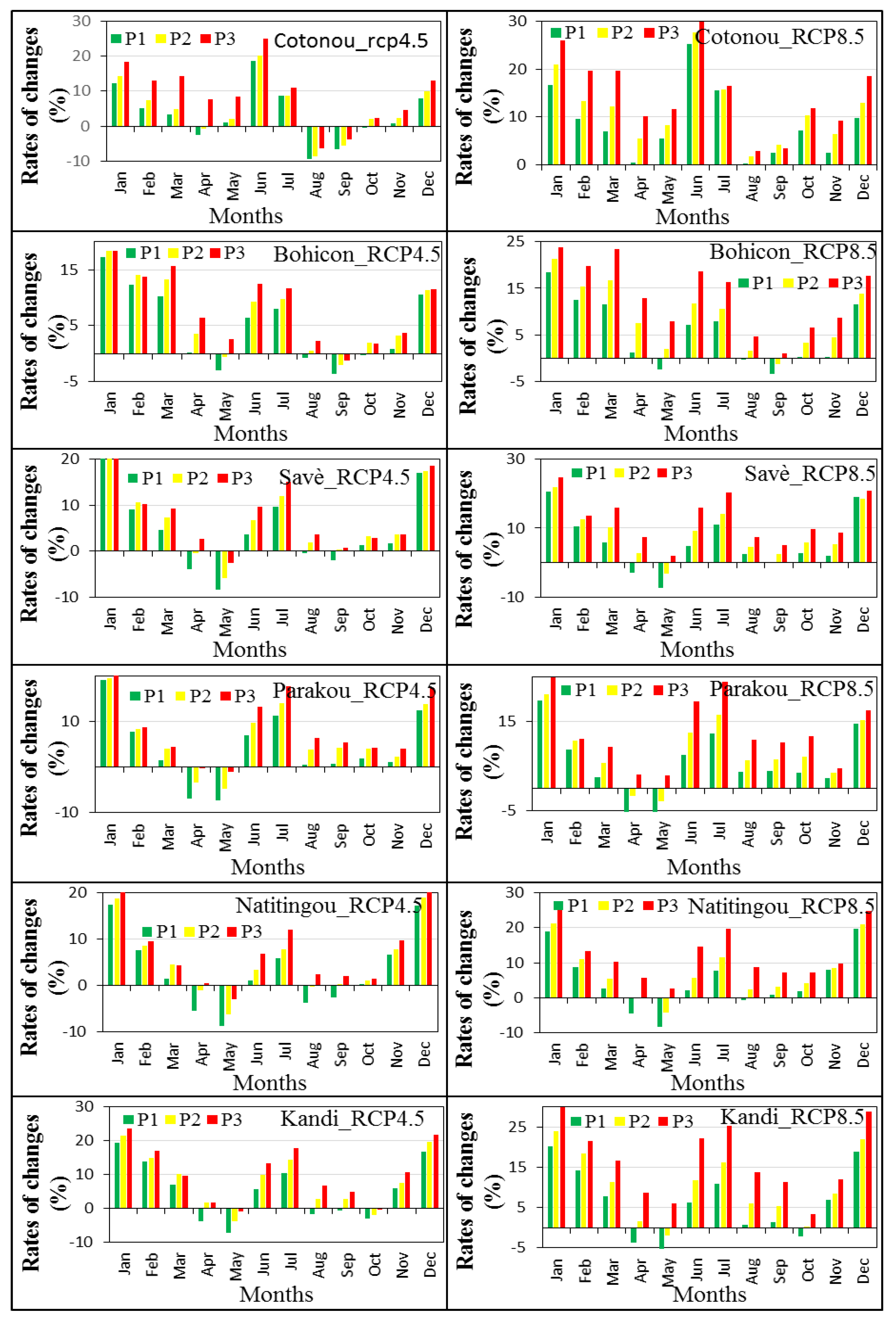
Given that PET estimates from these three RCMs converge, only PET estimates from a set of these models were used to analyze the changes of monthly PET. Figure 8 shows the rates of changes for all stations. According to the RCP4.5 scenario, there will be an increase of PET on January, February, March, June, July, November and December at all stations for the different projected periods. The rates of increase are rising according to the projected periods. Note that the large increases are obtained on January and December with rates of increase of about 20%. The months of April, May, August, September and October are characterized either by a slight decrease in PET, or by a slight increase according to the projected periods and the stations. The rates of change for these months range from −8 to 5%. Under the RCP8.5 scenario, there will be an increase in monthly PET at all stations and the different projected periods except for the April and May with little decrease especially for P1 and P2 projected periods. The rates of increase are higher for the months of January, February, March, June, July and December with rates of 15 to 25% of increase compared to the baseline period. As with the RCP4.5 scenario, the increases projected by the RCP8.5 scenario are increasing with projected periods. These results are consistent with those of many studies. Indeed, ref. [61] show increases in mean Penman–Monteith PET in all seasons, with the largest percentage increases in autumn (30–80%) and winter (30–60%) and smallest in spring (0–50%) and summer (20–40%). Ref. [66] use data from the HadRM3H RCM over Europe for 2080s projected and A2 scenario and show seasonal absolute differences between future and baseline Penman-Monteith PET. According to [5], seasonal or monthly changes are very different to annual changes of ECHAM5 model in Zhejiang Province, East China. This model projects an increases of PET in spring, autumn, and winter. They also found slight decreases near the coast in summer. HadCM3 projected decreases in spring and summer, while increases in PET in autumn and winter can be found. Ref. [67] also show that average PET is highest in summer, accounting for 39.4% and 38.5% of the annual PET under the historical and RCP 8.5 scenarios, respectively, followed in descending order by spring, autumn, and winter in 3H Plain region in China. They observed the largest increase with respect to the past in the southwest region with a change in magnitude of 25–32%, whereas the smallest increase was located in the northeast region (3–10%). As for autumn and winter, marked areas of low values are visible in the projected pattern of PET from the north to central parts of the region, whereas higher values can be found in eastern and southwestern regions.
4. Conclusions
The results of this study show a high variability of PET in Benin during the reference period with alternating periods of PET deficit and periods of PET excess. Projected PET indicates an increase in annual PET for the RCP4.5 and RCP8.5 scenarios. The RCP8.5 scenario leads to very significant increases in annual PET in future periods compared to the reference period, which will especially reach an increase between 10% and 20% at the end of the century. Under the RCP4.5 scenario, seasonal changes show a sharp increase in PET on January, February, June, July and December while in April, May, August, September and October, there is a small decrease of PET especially for P1 and P2 projected periods. Under the RCP8.5 scenario monthly PET increases. The increases in the months of January, February, June, July and December are high with about 20% while the increases of other months are low and less than 10%. The variability of the future monthly PET relative to the baseline period assumes that the seasonal variation of PET is too complicated. This confirms the fact that the trends observed during the baseline period vary from one month to other. This variability is related to the variation of the meteorological variables used to compute PET. It would be important to carry out a sensitivity study of PET to all meteorological variables in order to determine their relative influence on the variability of PET. It is also important to extend this study to the whole West African region.
Author Contributions
Ezéchiel Obada, Eric Adéchina Alamou, Amédée Chabi, Josué Zandagba and Abel Afouda designed the study, developed the methodology and wrote the manuscript; Ezéchiel Obada performed the field work, collected the data and conducted the computer analysis with Josué Zandagba and Amédée Chabi; Eric Adéchina Alamou and Abel Afouda supervised this part of the work.
Conflicts of Interest
The authors declare no conflict of interest.
References
- Liu, X.M.; Luo, Y.; Zhang, D.; Zhang, M.; Liu, C. Recent changes in pan-evaporation dynamics in China. Geophys. Res. Lett. 2011, 38, L13404. [Google Scholar] [CrossRef]
- McVicar, T.R.; Van Niel, T.G.; Li, L.T.; Hutchinson, M.F.; Mu, X.M.; Liu, Z.H. Spatially distributing monthly reference evapotranspiration and pan evaporation considering topographic influences. J. Hydrol. 2007, 338, 196–220. [Google Scholar] [CrossRef]
- Gu, S.; Tang, Y.; Cui, X.; Du, M.; Zhao, L.; Li, Y.; Xu, S.; Zhou, H.; Kato, T.; Qi, P.; et al. Characterizing evapotranspiration over a meadow ecosystem on the Qinghai-Tibetan Plateau. J. Geophys. Res. 2008, 113, D08118. [Google Scholar] [CrossRef]
- Van der Velde, Y.; Lyon, S.W.; Destouni, G. Data-driven regionalization of river discharges and emergent land cover-evapotranspiration relationships across Sweden. J. Geophys. Res. Atmos. 2013, 118, 2576–2587. [Google Scholar] [CrossRef]
- Xu, Y.P.; Pan, S.; Fu, G.; Tian, Y.; Zhang, X. Future potential evapotranspiration changes and contribution analysis in Zhejiang Province, East China. J. Geophys. Res. Atmos. 2014, 118, 2174–2192. [Google Scholar] [CrossRef]
- Allen, R.; Periera, L.; Raes, D.; Smith, M. FAO Irrigation and Drainage: Crop Evapotranspiration (Guidelines for Computing Crop Water Requirements); Food and Agriculture Organization of the United Nations (FAO): Rome, Italy, 1996; p. 56. [Google Scholar]
- Xu, C.; Gong, L.; Jiang, T.; Chen, D. Analysis of spatial distribution and temporal trend of reference evapotranspiration and pan evaporation in Changjiang (Yangtze River) catchment. J. Hydrol. 2006, 327, 81–93. [Google Scholar] [CrossRef]
- Bashir, M.; Tanakamaru, H.; Tada, A. Remote sensing-based estimates of evapotranspiration for managing scarce water resources in the Gezira Scheme, Sudan. J. Environ. Inform. 2009, 13, 86–92. [Google Scholar]
- Li, Z.; Zheng, F.; Liu, W. Spatiotemporal characteristics of reference evapotranspiration during 1961–2009 and its projected changes during 2011–2099 on the Loess Plateau of China. Agric. For. Meteorol. 2012, 154–155, 147–155. [Google Scholar] [CrossRef]
- Fan, Z.X.; Thomas, A. Spatiotemporal variability of reference evapotranspiration and its contributing climatic factors in Yunan Province, SW China, 1961–2004. Clim. Chang. 2013, 116, 309–325. [Google Scholar] [CrossRef]
- Alemu, H.; Senay, G.B.; Kaptue, A.T.; Kovalskyy, V. Evapotranspiration variability and its association with vegetation dynamics in the Nile Basin, 2002–2011. Remote Sens. 2014, 6, 5885–5908. [Google Scholar] [CrossRef]
- Valipour, M. Ability of Box-Jenkins Models to Estimate of Reference Potential Evapotranspiration (A Case Study: Mehrabad Synoptic Station, Tehran, Iran). IOSR J. Agric. Vet. Sci. 2012, 1, 1–11. [Google Scholar] [CrossRef]
- Valipour, M. Application of new mass transfer formulae for computation of evapotranspiration. J. Appl. Water Eng. Res. 2014, 2, 33–46. [Google Scholar] [CrossRef]
- Valipour, M. Study of different climatic conditions to assess the role of solar radiation in reference crop evapotranspiration equations. Arch. Agron. Soil Sci. 2014, 61, 679–694. [Google Scholar] [CrossRef]
- Valipour, M.; Gholami Sefidkouhi, M.A. Temporal analysis of reference evapotranspiration to detect variation factors. Int. J. Glob. Warm. 2017, in press. [Google Scholar] [CrossRef]
- Valipour, M. Importance of solar radiation, temperature, relative humidity, and wind speed for calculation of reference evapotranspiration. Arch. Agron. Soil Sci. 2015, 61, 239–255. [Google Scholar] [CrossRef]
- IPCC. Climate Change: The Climate Change. Contribution of the Working Group I to the Third Assessment Report of the Intergovernmental Panel on Climate Change; Cambridge University Press: Cambridge, UK, 2001. [Google Scholar]
- Valipour, M. Use of surface water supply index to assessing of water resources management in Colorado and Oregon, US. Adv. Agric. Sci. Eng. Res. 2013, 3, 631–640. [Google Scholar]
- Valipour, M. Global experience on irrigation management under different scenarios. J. Water Land Dev. 2017, 32, 95–102. [Google Scholar] [CrossRef]
- Trenberth, K.E. Atmospheric Moisture Residence Times and Cycling: Implications for Rainfall Rates and Climate Change. Clim. Chang. 1998, 39, 667–694. [Google Scholar] [CrossRef]
- Labat, D.; Goddéris, Y.; Probst, J.L.; Guyot, J.L. Evidence for Global Runoff Increase Related to Climate Warming. Adv. Water Res. 2004, 27, 631–642. [Google Scholar] [CrossRef] [Green Version]
- Huntington, T.G. Evidence for Intensification of the Global Water Cycle: Review and Synthesis. J. Hydrol. 2006, 319, 83–95. [Google Scholar] [CrossRef]
- Burt, T.P.; Shahgedanova, M. An historical record of evaporation losses since 1815 calculated using long-term observations from the Radcliffe Meteorological Station, Oxford, England. J. Hydrol. 1998, 205, 101–111. [Google Scholar] [CrossRef]
- Kay, A.L.; Bell, V.A.; Blyth, E.M.; Crooks, S.M.; Davies, H.N.; Reynard, N.S.A. Hydrological perspective on evaporation: Historical trends and future projections in Britain. J. Water Clim. Chang. 2013, 4, 193–208. [Google Scholar] [CrossRef]
- Onyutha, C. Statistical analyses of potential evapotranspiration changes over the period 1930–2012 in the Nile River riparian countries. Agric. For. Meteorol. 2016, 226–227, 80–95. [Google Scholar] [CrossRef]
- Ibrahim, B. Caractérisation des Saisons de Pluies au Burkina Faso Dans un Contexte de Changement Climatiques sur le Bassin de Nakambé. Thèse de Doctorat, Institut International d’Ingénierie de l’Eau et de l’Environnement (2iE), l’Université Pierre et Marie Curie, 2012; 234p. [Google Scholar]
- Jhajharia, D.; Pandey, P.K.; Dabral, P.P.; Kumar, R.; Choudhary, R. Variability in Temperature and Potential Evapotranspiration over West Siang in Arunachal Pradesh. Jour. Ind. Geil. Cong. 2015, 7, 37–43. [Google Scholar]
- Chattopdhyay, N.; Hulme, M. Evaporation and Potential Evapotranspiration in India under Conditions of Recent and Future Climate Change. Agric. For. Meteorol. 1997, 87, 55–73. [Google Scholar] [CrossRef]
- Moonen, A.C.; Ercoli, L.; Mariotti, M.; Masoni, A. Climate Change in Italy Indicated by Agro-meteorological Indices over 122 Years. Agric. For. Meteorol. 2002, 111, 13–27. [Google Scholar] [CrossRef]
- Chen, S.B.; Lui, Y.F.; Axel, T. Climatic change on the Tibetan Plateau: Potential evapotranspiration trends from 1961–2000. Clim. Chang. 2006, 76, 291–319. [Google Scholar]
- Yin, Y.; Wu, S.; Chen, G.; Dai, E. Attribution analyses of potential evapotranspiration changes in China since the 1960s. Theor. Appl. Climatol. 2010, 101, 19–28. [Google Scholar] [CrossRef]
- Xu, C.-Y.; Singh, V.P. Evaluation and generalization of radiation-based methods for calculating evaporation. Hydrol. Process. 2001, 15, 305–319. [Google Scholar] [CrossRef]
- Trajkovic, S. Temperature-based approaches for estimating reference evapotranspiration. J. Irrig. Drain. Eng. 2005, 131, 316. [Google Scholar] [CrossRef]
- Gong, L.; Xu, C.; Chen, D.; Halldin, S.; Chen, Y.D. Sensitivity of the Penman-Monteith reference evapotranspiration to key climatic variables in the Changjiang (Yangtze River) basin. J. Hydrol. 2006, 329, 620–629. [Google Scholar] [CrossRef]
- Nandagiri, L.; Kovoor, G. Performance evaluation of reference evapotranspiration equations across a range of Indian climates. J. Irrig. Drain. Eng. 2006, 132, 238. [Google Scholar] [CrossRef]
- Diodato, N.; Bellocchi, G. Modeling reference evapotranspiration over complex terrains from minimum climatological data. Water Resour. Res. 2007, 43, W05444. [Google Scholar] [CrossRef]
- Donohue, R.J.; McVicar, T.R.; Roderick, M.L. Assessing the ability of potential evaporation formulations to capture the dynamics in evaporative demand within a changing climate. J. Hydrol. 2010, 386, 186–197. [Google Scholar] [CrossRef]
- Judex, M.; Thamm, H.P. IMPETUS Atlas Benin Research Results 2000–2007, 3rd ed.; IMPETUS Project: Bonn, Germany, 2008. [Google Scholar]
- Van Vuuren, D.P.; Edmonds, J.; Kainuma, M.; Riahi, K.; Thomson, A.; Hibbard, K.; Hurtt, G.C.; Kram, T.; Krey, V.; Lamarque, J.F.; et al. The representative concentration pathways: An overview. Clim. Chang. 2011, 109, 5–31. [Google Scholar] [CrossRef]
- Clarke, L.; Edmonds, J.; Jacoby, H.; Pitcher, H.; Reilly, J.; Richels, R. CCSP Synthesis and Assessment Product 2.1, Part A: Scenarios of Greenhouse Gas Emissions and Atmospheric Concentrations; US Government Printing Office: Washington, DC, USA, 2007; 154p.
- Fujino, J.; Nair, R.; Kainuma, M.; Masui, T.; Matsuoka, Y. Multi-gas mitigation analysis on stabilization scenarios using AIM global model. Multigas Mitigation and Climate Policy. Energy J. 2006, 3, 343–353. [Google Scholar]
- Riahi, K.; Gruebler, A.; Nakicenovic, N. Scenarios of long-term socio-economic and environmental development under climate stabilization. Technol. Forecast. Soc. Chang. 2007, 74, 887–935. [Google Scholar] [CrossRef]
- Christensen, O.B.; Drews, M.; Christensen, J.H. The HIRHAM Regional Climate Model Version 5. Available online: http://orbit.dtu.dk/fedora/objects/orbit:118724/datastreams/file_8c69af6e-acfb-4d1aaa53–73188c001d36/content (accessed on 15 February 2017).
- Jacob, D.; Bärring, L.; Christensen, O.B.; Christensen, J.H.; Hagemann, S.; Hirschi, M.; Kjellström, E.; Lenderink, G.; Rockel, B.; Schär, C.; et al. An inter-comparison of regional climate models for Europe: Design of the experiments and model performance. Clim. Chang. 2007, 81, 31–52. [Google Scholar] [CrossRef]
- Samuelsson, P.; Jones, C.G.; Willén, U.; Ullerstig, A.; Gollvik, S.; Hansson, U.; Kjellström, E.; Nikulin, G.; Wyser, K. The Rossby Centre regional climate model RCA3: Model description and performance. Tellus A 2011, 63, 4–23. [Google Scholar] [CrossRef]
- Mann, H.B. Nonparametric tests against trend. Econometrica 1945, 13, 245–259. [Google Scholar] [CrossRef]
- Kendall, M. Rank Correlation Methods; Oxford University Press: Oxford, UK, 1948. [Google Scholar]
- Partal, T.; Kahya, E. Trend analysis in Turkish precipitation data. Hydrol. Process. 2006, 20, 2011–2026. [Google Scholar] [CrossRef]
- Yu, X.; Zhao, G.; Zhao, W.; Yan, T.; Yuan, X. Analysis of Precipitation and Drought Data in Hexi Corridor, Northwest China. Hydrology 2017, 4, 29. [Google Scholar] [CrossRef]
- Wetterhall, F.; Pappenberger, F.; He, Y.; Freer, J.; Cloke, H. Conditioning model output statistics of regional climate model precipitation on circulation patterns. Nonlinear Process. Geophys. 2012, 19, 623–633. [Google Scholar] [CrossRef] [Green Version]
- Fang, G.H.; Yang, J.; Chen, Y.N.; Zammit, C. Comparing bias correction methods in downscaling meteorological variables for a hydrologic impact study in an arid area in China. Hydrol. Earth Syst. Sci. 2015, 19, 2547–2559. [Google Scholar] [CrossRef] [Green Version]
- Déqué, M. Frequency of precipitation and temperature extreme over France in an anthropogenic scenario: Model results and statistical correction according to observed values. Glob. Planet Chang. 2007, 57, 16–26. [Google Scholar] [CrossRef]
- Sennikovs, J.; Bethers, U. Statistical downscaling method of regional climate model results for hydrological modelling. In Proceedings of the 18th World IMACS Congress and MODSIM09 International Congress on Modelling and Simulation, Cairns, Australia, 13–17 July 2009. [Google Scholar]
- Michelangeli, P.A.; Vrac, M.; Loukos, H. Probabilistic downscaling approaches: Application to wind cumulative distribution function. Geophys. Res. Lett. 2009, 36, L11708. [Google Scholar] [CrossRef]
- Piani, C.; Haerter, J.; Coppola, E. Statistical bias correction for daily precipitation in regional climate models over Europe. Theor. Appl. Climatol. 2010, 99, 187–192. [Google Scholar] [CrossRef]
- Trenberth, K.; Dai, A.; Rasmussen, R.; Parsons, D. The changing character of precipitation. Bull. Am. Meteorol. Soc. 2003, 84, 1205–1217. [Google Scholar] [CrossRef]
- Weedon, G.P.; Gomes, S.; Viterbo, P.; Shuttleworth, W.J.; Blyth, E.; Österle, H.; Adam, J.C.; Bellouin, N.; Boucher, O.; Best, M. Creation of the WATCH Forcing Data and Its use to assess global and regional reference crop evaporation over land during the twentieth century. J. Hydrometeorol. 2011, 12, 823–848. [Google Scholar] [CrossRef]
- Thomas, A. Spatial and temporal characteristics of potential evapotranspiration trends over China. Int. J. Climatol. 2000, 20, 381–396. [Google Scholar] [CrossRef]
- Yin, Y.; Wu, S.; Zhao, D. Past and future spatiotemporal changes in evapotranspiration and effective moisture on the Tibetan Plateau. J. Geophys. Res. Atmos. 2013, 118, 10850–10860. [Google Scholar] [CrossRef]
- Arnell, N.W. Uncertainty in the relationship between climate forcing and hydrological response in UK catchments. Hydrol. Earth Syst. Sci. 2011, 15, 897–912. [Google Scholar] [CrossRef]
- Fowler, H.J.; Tebaldi, C.; Blenkinsop, S. Probabilistic estimates of climate change impacts on flows in the river Eden, Cumbria. In Proceedings of the British Hydrological Society 10th National Hydrology Symposium, Exeter, UK, 15–17 September 2008. [Google Scholar]
- Scheff, J. Reference Evapotranspiration from Standard Archived GCM Output: A Proof of Concept. 2011. Available online: www.atmos.washington.edu/~jack/PotEvapGCM.ps (assessed on 18 April 2017).
- King, D.A.; Bachelet, D.M.; Symstad, A.J.; Ferschweiler, K.; Hobbins, M. Estimation of potential evapotranspiration from extraterrestrial radiation, air temperature and humidity to assess future climate change effects on the vegetation of the Northern Great Plains, USA. Ecol. Model. 2015, 297, 86–97. [Google Scholar] [CrossRef]
- Scheff, J.; Frierson, D.M. Scaling potential evapotranspiration with greenhouse warming. J. Clim. 2013, 27, 1539–1558. [Google Scholar] [CrossRef]
- Feng, S.; Fu, Q. Expansion of global dry lands under warming climate. Atmos. Chem. Phys. 2013, 13, 10081–10094. [Google Scholar] [CrossRef]
- Ekstrom, M.; Jones, P.D.; Fowler, H.J.; Lenderink, G.; Buishand, T.A.; Conway, D. Regional climate model data used within the SWURVE project 1: Projected change in seasonal patterns and estimation of PET. Hydrol. Earth Syst. Sci. 2007, 11, 1069–1083. [Google Scholar] [CrossRef]
- Liu, Q.; Yan, C.; Ju, H.; Garré, S. Impact of climate change on potential evapotranspiration under a historical and future climate scenario in the Huang-Huai-Hai Plain, China. Theor. Appl. Climatol. 2017, 1–15. [Google Scholar] [CrossRef]
Figure 1.
Study area.
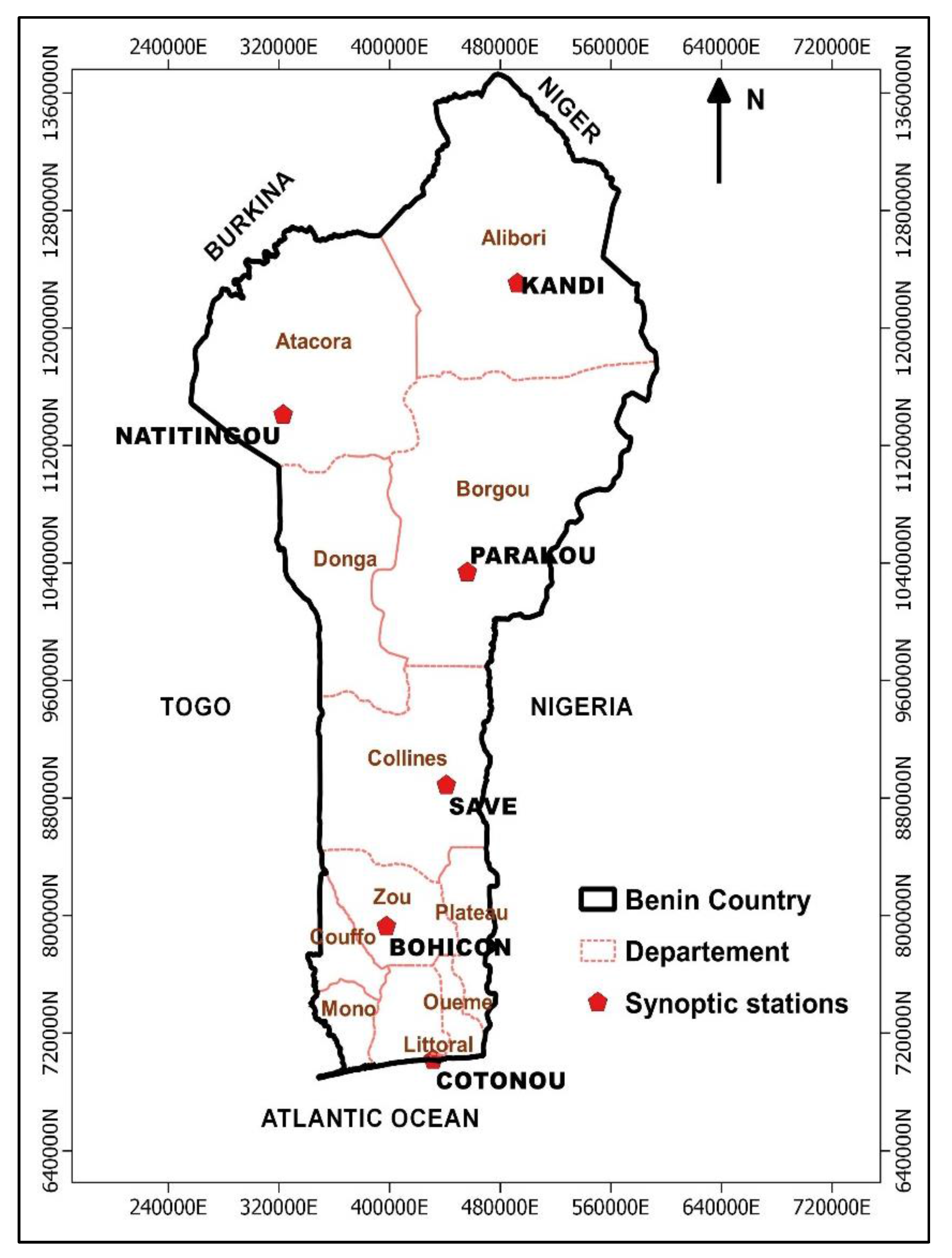
Figure 2.
Evolution of Annual PET index over the reference period.

Figure 3.
Observed and simulated (no bias corrected) annual PET.

Figure 4.
Observed and simulated (bias corrected with EQM method) annual PET.
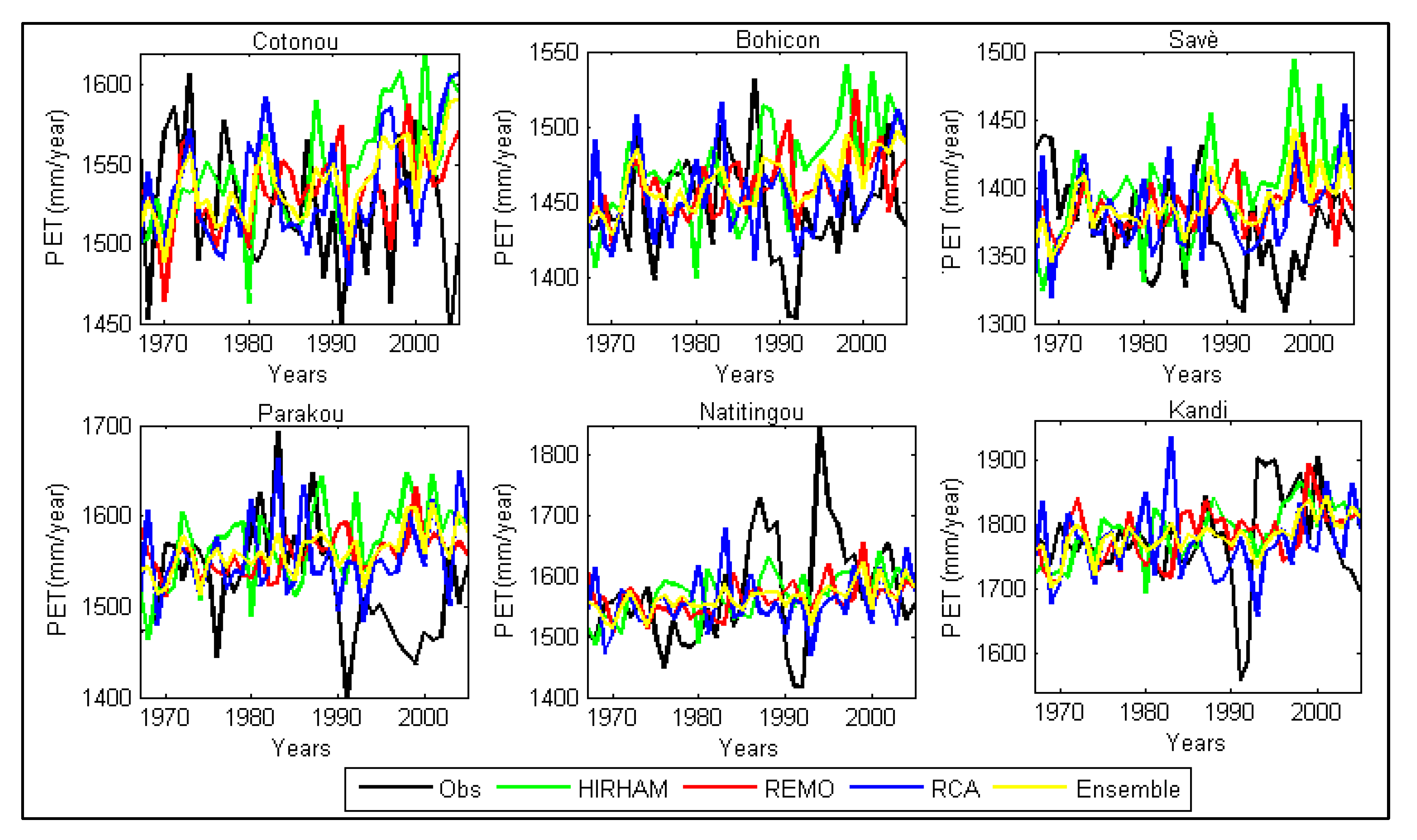
Figure 5.
Evolution of annual PET from 1967 to 2100 under RCP4.5 scenario.
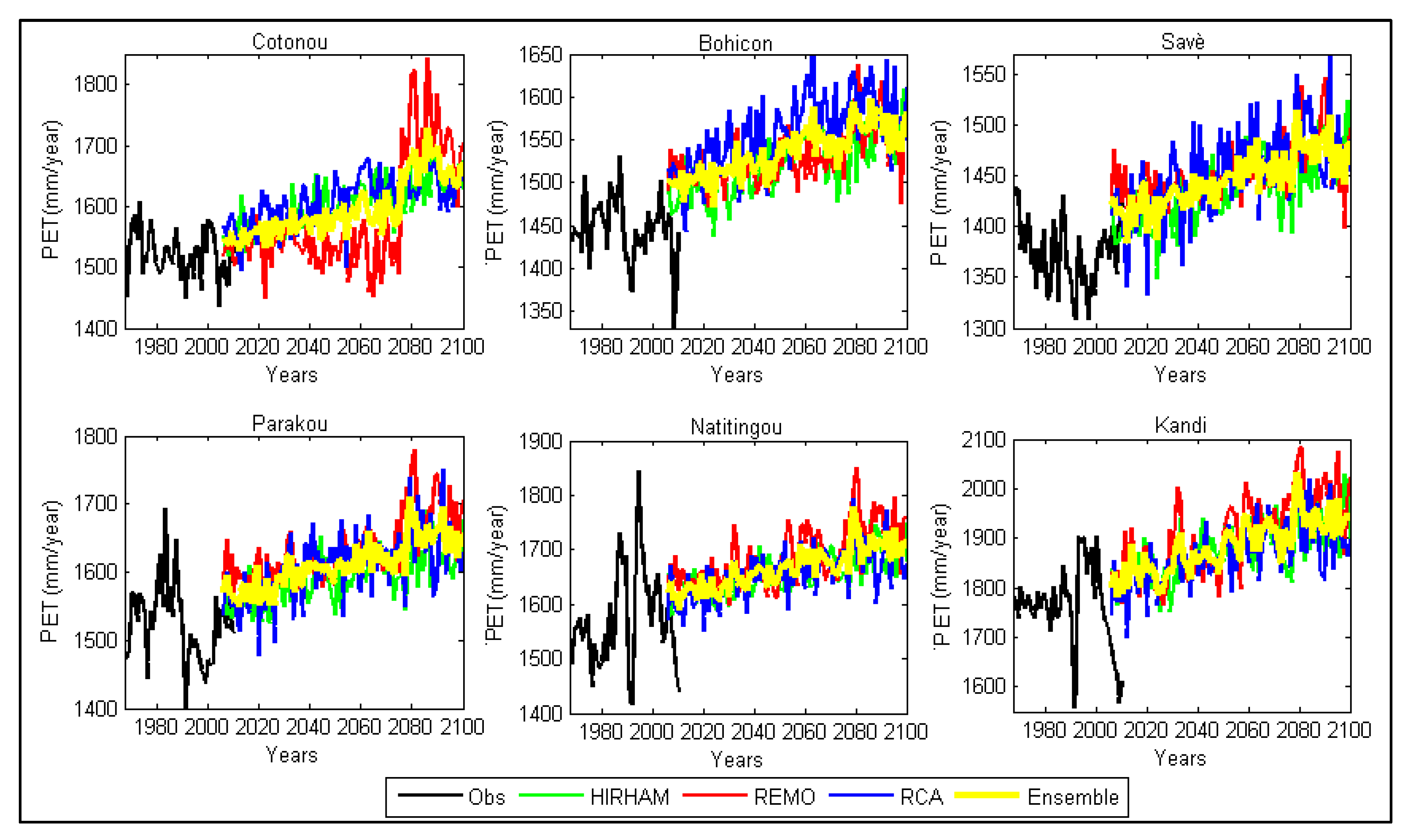
Figure 6.
Evolution of annual PET from 1967 to 2100 under RCP8.5 scenario.

Figure 7.
Rates of changes in future annual PET relative to the baseline period.
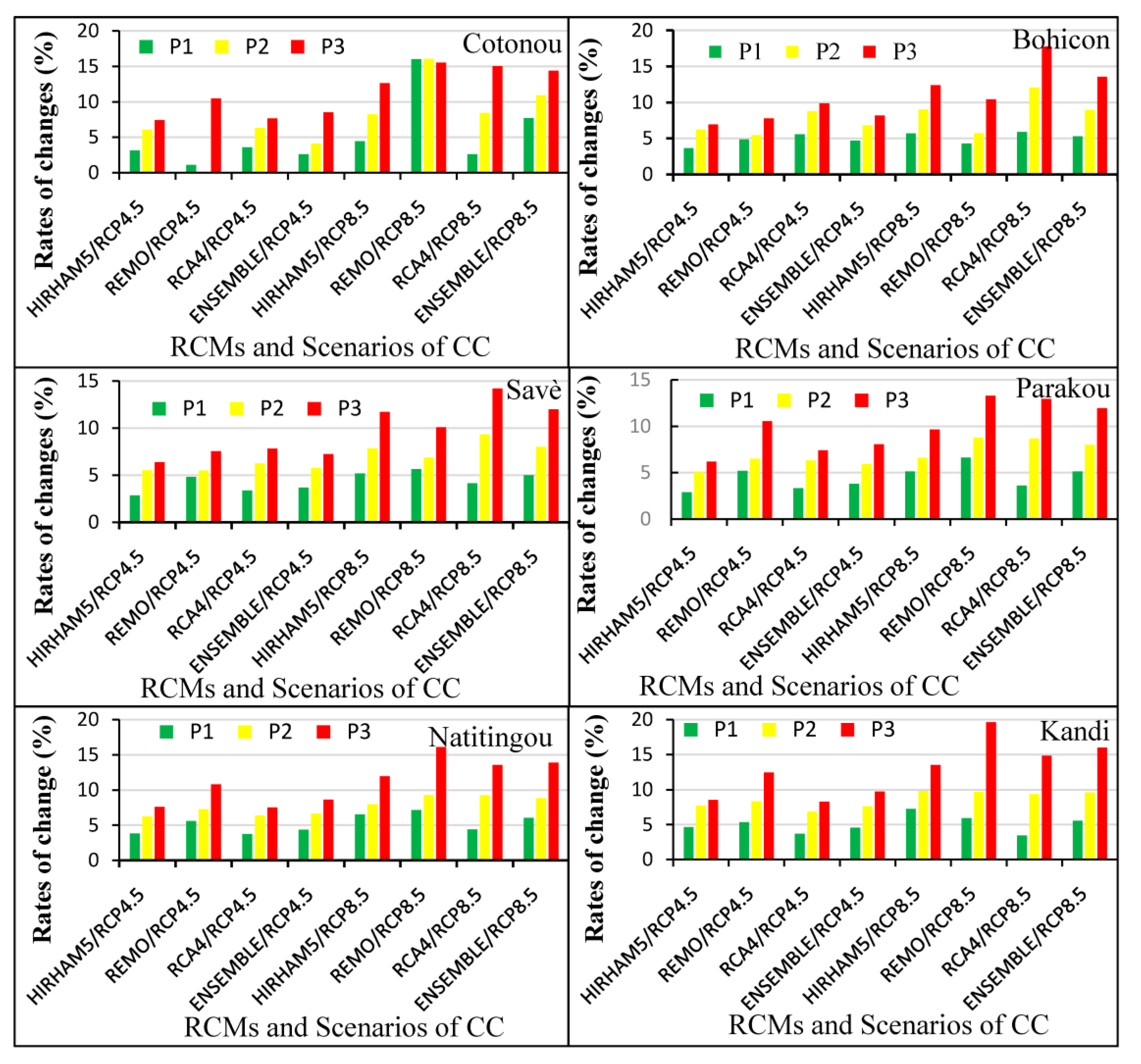
Figure 8.
Rates of changes in future monthly PET relative to the baseline period.


Table 1.
Geographical descriptions of meteorological stations in the study area.
| Station | Longitude (°C) | Latitude (°C) | Elevation (m) |
|---|---|---|---|
| Cotonou | 2.38 | 6.35 | 4 |
| Bohicon | 2.07 | 7.17 | 166 |
| Savè | 2.47 | 8.03 | 198 |
| Parakou | 2.6 | 9.35 | 392 |
| Natitingou | 1.38 | 10.32 | 460 |
| Kandi | 2.93 | 11.13 | 290 |
Table 2.
Main characteristics of the RCMs.
| Model (RCM) | Institution | Driving GCM | Horizontal Resolution | No. of Vertical Levels | Simulation Period | Reference |
|---|---|---|---|---|---|---|
| HIRHAM5 | DMI | GFDL-ESM2M | 50 km | 31 | 1951–2100 | [43] |
| REMO | CSC | MPI-ESM-LR | 50 km | 27 | 1951–2100 | [44] |
| RCA4 | SMHI | EC-EARTH | 50 km | 40 | 1951–2100 | [45] |
Table 3.
Zs values of Mann-Kendall test on monthly and annual data during 1981–2010.
| Month | Cotonou | Bohicon | Savè | Parakou | Natitingou | Kandi | |
|---|---|---|---|---|---|---|---|
| January | −0.07 | −1.75 | −0.64 | −1.57 | −0.14 | −0.57 | |
| February | +0.57 | −1.78 | +0.39 | −1.68 | −0.54 | −0.61 | |
| March | −0.21 | −1.43 | +0.39 | −2.50 * | −0.82 | −0.86 | |
| April | −2.14 * | −1.53 | −0.50 | −3.21 * | −0.46 | −1.21 | |
| May | −0.82 | −0.89 | −1.07 | −2.11 * | −1.11 | −2.00 * | |
| June | −0.82 | −2.18 * | +1.36 | −1.14 | −0.68 | −2.32 * | |
| July | +1.43 | +1.43 | +2.71 * | +0.93 | −0.46 | −2.03 * | |
| August | +0.86 | −0.75 | −0.21 | −0.96 | −1.11 | −2.71 * | |
| September | +1.71 | −0.39 | +1.36 | −0.29 | −0.96 | −2.11 * | |
| October | −0.86 | −0.82 | +2.28 * | −0.14 | −0.50 | −1.82 | |
| November | −0.36 | −0.11 | +2.78 * | +0.46 | −1.07 | −0.61 | |
| December | +3.00 * | +2.32 * | +2.39 * | +1.00 | −0.32 | +0.54 | |
| Annual | +0.18 | −0.96 | +1.53 | −1.71 | −0.96 | −1.71 | |
* Indicates statistically significant trend at 95%.
Table 4.
Bias correction performances.
| Calibration | Validation | |||||||||||||||||
|---|---|---|---|---|---|---|---|---|---|---|---|---|---|---|---|---|---|---|
| HIRHAM 5 | REMO | RCA4 | HIRHAM 5 | REMO | RCA4 | |||||||||||||
| Station | Raw | Scaling | EQM | Raw | Scaling | EQM | Raw | Scaling | EQM | Raw | Scaling | EQM | Raw | Scaling | EQM | Raw | Scaling | EQM |
| MAE | ||||||||||||||||||
| Cotonou | 0.91 | 0.85 | 0.80 | 0.90 | 0.89 | 0.77 | 0.96 | 0.74 | 0.77 | 0.95 | 0.85 | 0.80 | 0.89 | 0.89 | 0.77 | 1.01 | 0.75 | 0.79 |
| Bohicon | 1.02 | 0.90 | 0.70 | 1.00 | 1.01 | 0.65 | 1.21 | 0.72 | 0.62 | 1.09 | 0.93 | 0.72 | 1.00 | 1.03 | 0.66 | 1.27 | 0.73 | 0.61 |
| Savè | 1.16 | 0.91 | 0.72 | 1.09 | 1.08 | 0.70 | 1.38 | 0.77 | 0.70 | 1.25 | 0.92 | 0.73 | 1.12 | 1.10 | 0.70 | 1.45 | 0.76 | 0.67 |
| Parakou | 1.10 | 0.96 | 0.80 | 0.95 | 0.96 | 0.73 | 1.39 | 0.86 | 0.82 | 1.27 | 1.03 | 0.85 | 1.00 | 1.03 | 0.78 | 1.56 | 0.87 | 0.82 |
| Natitingou | 1.29 | 1.12 | 0.86 | 1.06 | 1.04 | 0.8 | 1.44 | 0.94 | 0.87 | 1.31 | 1.15 | 0.9 | 1.02 | 1.01 | 0.81 | 1.39 | 0.96 | 0.89 |
| Kandi | 1.34 | 1.16 | 0.98 | 0.99 | 0.99 | 0.87 | 1.32 | 0.97 | 1.04 | 1.39 | 1.18 | 1.03 | 1.02 | 1.02 | 0.92 | 1.34 | 1.01 | 1.07 |
| RMSE | ||||||||||||||||||
| Cotonou | 0.36 | 0.00 | 0.00 | 0.34 | 0.00 | 0.00 | 0.74 | 0.00 | 0.00 | 0.52 | 0.16 | 0.16 | 0.26 | 0.07 | 0.07 | 0.81 | 0.07 | 0.08 |
| Bohicon | 0.49 | 0.00 | 0.02 | 0.32 | 0.00 | 0.01 | 1.11 | 0.00 | 0.00 | 0.67 | 0.18 | 0.16 | 0.21 | 0.11 | 0.09 | 1.17 | 0.07 | 0.06 |
| Savè | 0.79 | 0.00 | 0.01 | 0.09 | 0.00 | 0.00 | 1.30 | 0.00 | 0.00 | 0.99 | 0.20 | 0.17 | 0.20 | 0.11 | 0.10 | 1.39 | 0.10 | 0.09 |
| Parakou | 0.61 | 0.00 | 0.01 | 0.13 | 0.00 | 0.01 | 1.27 | 0.00 | 0.00 | 0.94 | 0.33 | 0.31 | 0.12 | 0.25 | 0.24 | 1.49 | 0.22 | 0.22 |
| Natitingou | 0.72 | 0.00 | 0.01 | 0.16 | 0.00 | 0.01 | 1.30 | 0.00 | 0.00 | 0.72 | 0.00 | 0.03 | 0.11 | 0.05 | 0.07 | 1.19 | 0.11 | 0.11 |
| Kandi | 0.76 | 0.00 | 0.01 | 0.08 | 0.00 | 0.01 | 1.09 | 0.00 | 0.00 | 0.85 | 0.09 | 0.07 | 0.03 | 0.05 | 0.04 | 1.05 | 0.04 | 0.04 |
© 2017 by the authors. Licensee MDPI, Basel, Switzerland. This article is an open access article distributed under the terms and conditions of the Creative Commons Attribution (CC BY) license (http://creativecommons.org/licenses/by/4.0/).
Share and Cite
MDPI and ACS Style
Obada, E.; Alamou, E.A.; Chabi, A.; Zandagba, J.; Afouda, A. Trends and Changes in Recent and Future Penman-Monteith Potential Evapotranspiration in Benin (West Africa). Hydrology 2017, 4, 38. https://doi.org/10.3390/hydrology4030038
AMA Style
Obada E, Alamou EA, Chabi A, Zandagba J, Afouda A. Trends and Changes in Recent and Future Penman-Monteith Potential Evapotranspiration in Benin (West Africa). Hydrology. 2017; 4(3):38. https://doi.org/10.3390/hydrology4030038
Chicago/Turabian StyleObada, Ezéchiel, Eric Adéchina Alamou, Amedée Chabi, Josué Zandagba, and Abel Afouda. 2017. "Trends and Changes in Recent and Future Penman-Monteith Potential Evapotranspiration in Benin (West Africa)" Hydrology 4, no. 3: 38. https://doi.org/10.3390/hydrology4030038
Note that from the first issue of 2016, this journal uses article numbers instead of page numbers. See further details here.