Evaluation of Gridded Precipitation Data Products for Hydrological Applications in Complex Topography

Department of Geography, Ludwig-Maximilians-Universität München (LMU), 80333 Munich, Germany
*
Author to whom correspondence should be addressed.
Hydrology 2017, 4(4), 53; https://doi.org/10.3390/hydrology4040053
Submission received: 6 October 2017
/
Revised: 10 November 2017
/
Accepted: 11 November 2017
/
Published: 16 November 2017
Abstract
:Accurate spatial and temporal representation of precipitation is of utmost importance for hydrological applications. Uncertainties in available data sets increase with spatial resolution due to small-scale processes over complex terrain. As previous studies revealed high regional differences in the performance of gridded precipitation data sets, it is important to assess the related uncertainties at the catchment scale, where these data sets are typically applied, e.g., for hydrological modeling. In this study, the uncertainty of eight gridded precipitation data sets from various sources is investigated over an alpine catchment. A high resolution reference data set is constructed from station data and applied to quantify the contribution of spatial resolution to the overall uncertainty. While the results demonstrate that the data sets reasonably capture inter-annual variability, they show large seasonal differences. These increase for daily indicators assessing dry and wet spells as well as heavy precipitation. Although the higher resolution data sets, independent of their source, show a better agreement, the coarser data sets showed great potential especially in the representation of the overall climatology. To bridge the gaps in data scarce areas and to overcome the issues with observational data sets (e.g., undercatch and station density) it is important to include a variety of data sets and select an ensemble for a robust representation of catchment precipitation. However, the study highlights the importance of a thorough assessment and a careful selection of the data sets, which should be tailored to the desired application.
1. Introduction
Precipitation plays an important role in the hydrological cycle and is one of the most widely used climate variables [1,2]. While there is a clear link between the amount, intensity, and distribution of precipitation to various processes in the ecosystem [3], this relation is nonlinear, and heavy precipitation does not necessarily result in high river discharge [4,5]. Additionally, the link of heavy precipitation and flood occurrence is challenging to assess and quantify [6]. Nevertheless, accurate assessment of precipitation is of utmost importance as it provides the meteorological input for hydrological and other impact models and studies. As precipitation varies greatly in space and time [7,8], gridded precipitation information in high temporal and spatial resolution is required. The need for such high-resolution data sets is crucial and not only limited to hydrological applications, but many other fields, such as evaluation of the performance of climate simulations and possible detection and adjustment of model biases. The need for high resolution is increased over areas with complex topography with high spatial variability [9].
Available gridded precipitation datasets differ in their domain size, spatial and temporal resolution, and originate from different sources and methods. Usually, a trade-off between spatial resolution and domain size must be made. While global and continental data sets, provided e.g., through the National Oceanic & Atmospheric Administration (NOAA) [10], the European Centre for Medium-Range Weather Forecasts (ECMWF) [11] and the German Weather Service (DWD) [12], provide information on precipitation over a large domain and cover a large time period, they lack the high spatial resolution required for regional or catchment scale studies. High-resolution data sets are usually only available on a country level [13] or cover a specific geographical region [14]. These data sets are either reanalysis products [10,11,15,16,17], derived through remote sensing [18,19] or interpolated station observations [12,14,20]. Most of these data sets use station data either directly, or assimilate observed precipitation at some stage. The density of the included stations differs greatly between, but also within the data sets, restricting the effective resolution and spatial consistency [21]. Recent efforts were made to merge different data sets to achieve a better representation and combining the advantages of each data set [22], as well as collecting sub-daily station observations [23] to increase the temporal resolutions. However, observations are prone to severe undercatch of precipitation, which is amplified in case of solid precipitation and over mountainous areas [21,24,25]. Therefore, there is merit in including data sets from a variety of sources for a robust estimation of reference precipitation.
Various studies to assess the performance of these data sets were carried out in recent years, revealing considerable differences between the products. Most of these studies focus either on global, continental, or regional performance assessment often aiming in the evaluation of Regional Climate Model (RCM) performance [2,26]. Regional studies assess the benefit of higher resolution and consequently a better topographic representation, the issues of station density and the representation of regional weather phenomena [21]. Detailed source specific assessment showed limitations in the representation of several weather patterns for reanalysis data sets [27] and the restriction of satellite information under specific cloud cover conditions [15,28]. Gridded precipitation data products are very often applied as meteorological input for hydrological modeling exercises in data scarce areas to bridge the data gap at the catchment or smaller regional scale [29,30]. It is therefore important to also assess the performance of the data set at smaller scales over hydrological basins. Some studies detect the deviations on the catchment scale; however they focus on reanalysis [27] or selected regional data sets [31]. Additional efforts were carried out in the past focusing on 3-hourly and daily error analysis for satellite precipitation products over alpine catchments. They revealed large errors especially in the summer months and showed the difficulties to adequately address errors in satellite products with respect to the station density of in situ measurements [32]. Other studies identified the impact of different satellite precipitation products on the reproduction of flood events in Northern Italy. These studies showed both the potential and advantages of these data products, but also their limitations [33,34].
However, there is still a need to evaluate long-term uncertainties and differences in existing precipitation products on the catchment scale, and exploiting as many of the available products as possible from different sources. It is important to assess not only the climatology, but also the daily extremes. This study contributes to recent findings by including an ensemble of eight available gridded precipitation data sets derived from observations and through reanalysis or remote sensing. These are evaluated against a high-resolution reference grid derived from local observations over a river basin for the period 1989–2008, with a focus on hydrological implications. Therefore, the comprehensive assessment does not only focus on the general climatology, but also on dry and wet spells, as well as extreme precipitation on the catchment scale. The study area is the catchment of the Adige in located in the southern part of the Alps in Northern Italy, covering an area of 12,100 km2. This catchment is selected due to a relatively high network of observation stations, and the challenging orography for the comparison with the ensemble of precipitation data sets. Due to the complex topography, the uncertainty introduced by the spatial resolution of the data sets was of special interest in this study. The overall purpose of this study was motivated from the application point of view, rather than atmospheric assessment of regional patterns. It is clear, that the outcomes of this study are highly regionally dependent and cannot be transferred to other catchments, but will give insights in local performance and uncertainties of precipitation data sets, especially over an alpine catchment.
2. Study Area
The focus of this study was the catchment of the Adige located in Northern Italy. The catchment, shown in Figure 1, covers an area of 12,100 km2. The Adige River stretches over a length of 409 km from the Southern Alps to the Adriatic Sea, passing three Italian provinces.
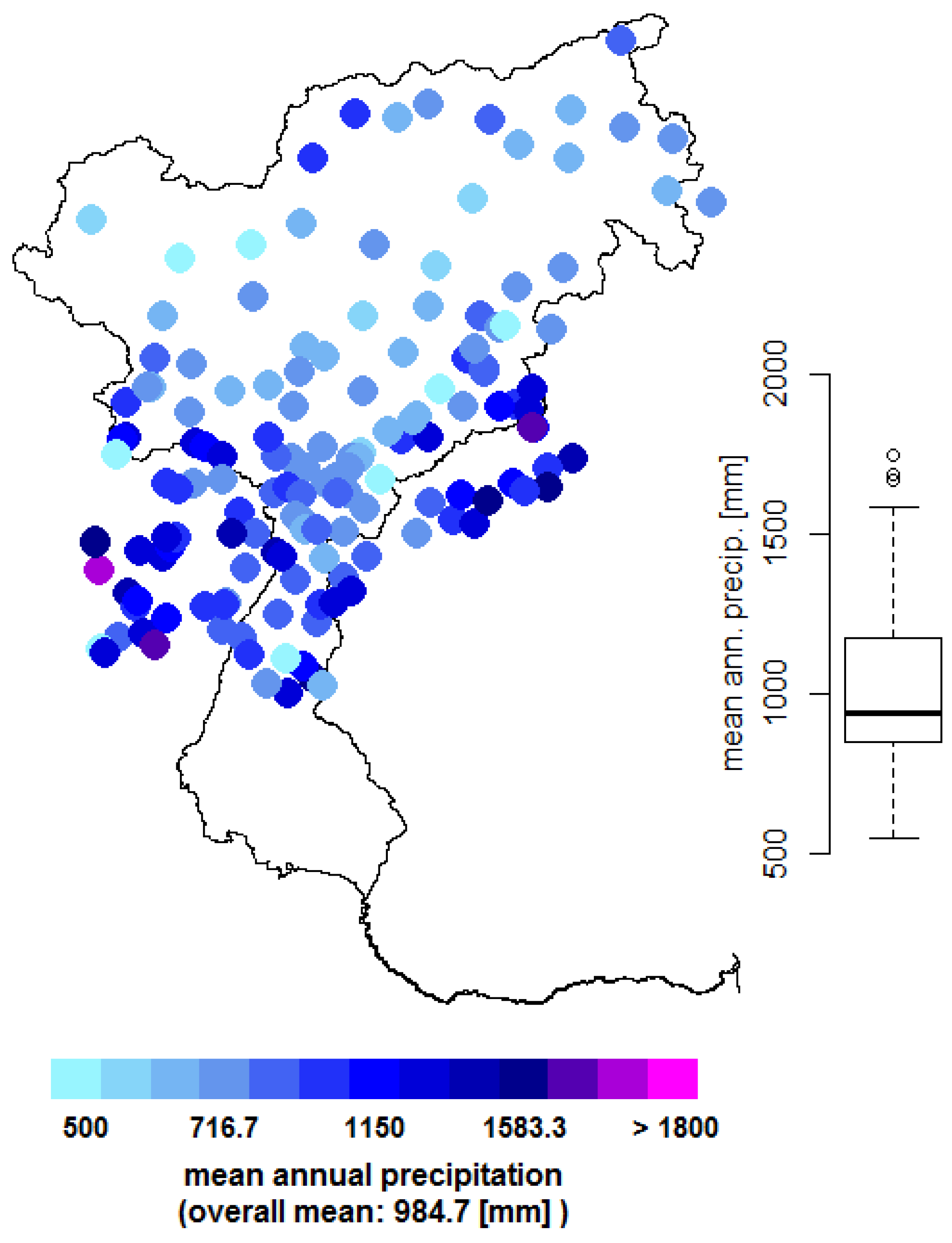
The area is characterized by a humid climate with annual mean precipitation ranging from 500 mm in the inner-Alpine dry areas, such as the Venosta valley [14,35], to 1600 mm. Precipitation distribution shows a pronounced summer peak and relatively dry winters [36]. An overview of the observed mean annual precipitation at the available stations is presented in Figure 2. The area is characterized by strong elevation differences ranging from sea level to 3865 m, as presented in Figure 1. The hydrology is characterized by snow and glacier melting in the spring months, and intense precipitation events in summer [36]. Discharge is used for irrigation of intensive agriculture - mainly fruit trees - and through various touristic activities. Additionally, 30 major reservoirs used for power generation are operated in the area, increasing pressure on ecosystems due to altered hydrology [37].
3. Data Sets and Methods
3.1. Construction of the High-Resolution Reference Data Set
Daily precipitation data for the period 1989–2008 derived from gauge measurements was available over the catchment. The station network for the study area covers a total of 153 stations as presented in Figure 2; however the temporal and orographic coverage varies considerably. Apart from the temporal coverage, the spatial distribution also varies strongly throughout the area, as shown in Figure 2. Most stations are located in the central to southern part of the catchment while especially the north-western part is sparsely covered. The southernmost part of the catchment is only covered by far away stations, as local stations were not available.
As the study aims in evaluating gridded precipitation products, the meteorological interpolation module of the hydrological model Water Flow and Balance Simulation Model (WaSiM, [38]) was chosen for the construction of the precipitation grid with a spatial resolution of 1 km and daily time step. This procedure was selected as it is computationally efficient, and furthermore, the resulting data set will serve as meteorological forcing of this hydrological model in consecutive studies. Additionally, the module ‘regional superposition’ allows for overlaying and combining multiple interpolation methods over various areas to consider topographic effects and specifications of the catchment. In the following the selected method is briefly described, whereas for a detailed insight, it is referred to in the technical report [38].
The precipitation at each grid cell was calculated based on the four nearest stations in respective quadrants, ideally on a regular grid. If no station was available in the respective quadrant, the scheme automatically switched to Inverse Distance Weighing (IDW), which is also widely used for interpolation of meteorological variables [39,40,41], and can be helpful in areas with low station density [42]. For mountainous areas, elevation dependent regression was applied to account for topographic effects. Here, the inversion levels were calibrated to better represent the characteristics of the catchment. In this study, in a first step, bilinear interpolation and elevation dependent regression were applied separately over the entire catchment. In a second step, the regional superposition module was applied to combine both approaches. In this way topographic effects could be captured, but were not overestimated, and the inner-Alpine dry areas were better captured compared to exclusive elevation-dependent regression. Additionally, the residuals for the regression were calculated for various sub regions to achieve better performance, and a better representation of the observed fields. The final grid was constructed for the period 1989–2008, which represents the maximum temporal coverage of the analyzed gridded data products presented in Section 3.3. All analyses presented in this study refer to this time frame only. The grid will be referred to as ADG-1KGPR, representing the gridded precipitation over the Adige domain with a 1 km grid size.
3.2. Performance Validation of the Constructed Reference Grid
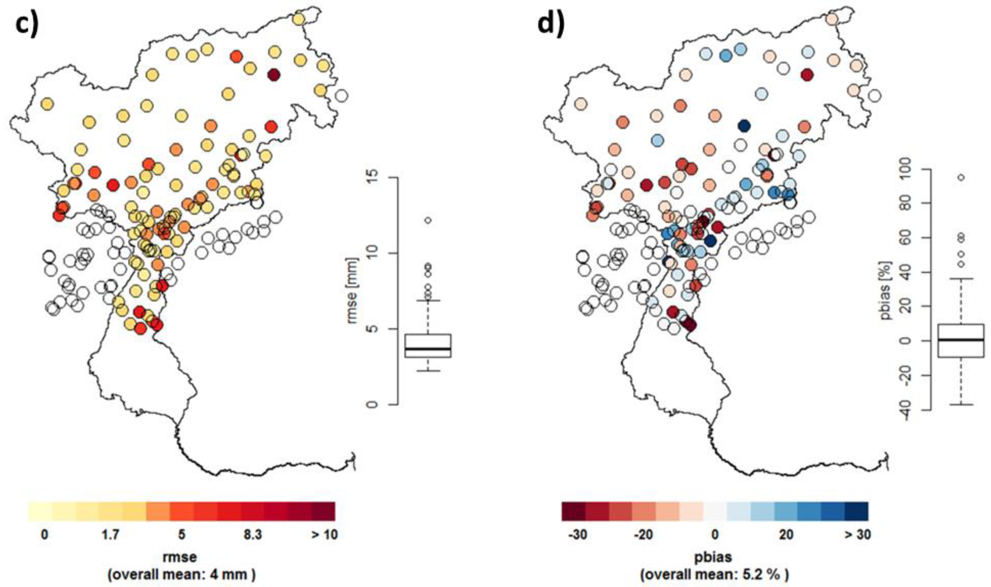
To assess the performance of the grid, a leave-one-out-cross-validation (LOOCV) approach was applied to allow for best-possible representation of the observed precipitation. Three main indicators were calculated to assess the performance of the interpolation method; The Percent Bias (PBIAS) assesses the tendency of the modeled data to exceed or underestimate the observed data in percent, hence the optimal value is zero. The Root Mean Square Error (RMSE) and the Mean Absolute Error (MAE) are two widely used indicators when it comes to model performance assessment in meteorology and other fields [43,44]. Figure 3 shows the presented evaluation criteria at the precipitation gauges and their corresponding grid cells in the interpolated 1 km gridded result. Stations outside the catchment are left out of the analysis to avoid confusing results and just presented as empty circles in the figure. Figure 3a represents the MAE*, which is the MAE based on all dates for the period 1989–2008, whereas Figure 3b shows the MAE, which is based only on days with precipitation occurrence. Therefore MAE showed higher values as MAE*, as the absolute error at days with no or only low precipitation was relatively small. Figure 3c shows the RMSE, and in Figure 3d, the corresponding PBIAS is shown. Both mean RMSE and MAE show similar or better results as comparable studies over various study areas [40,42,44,45,46].
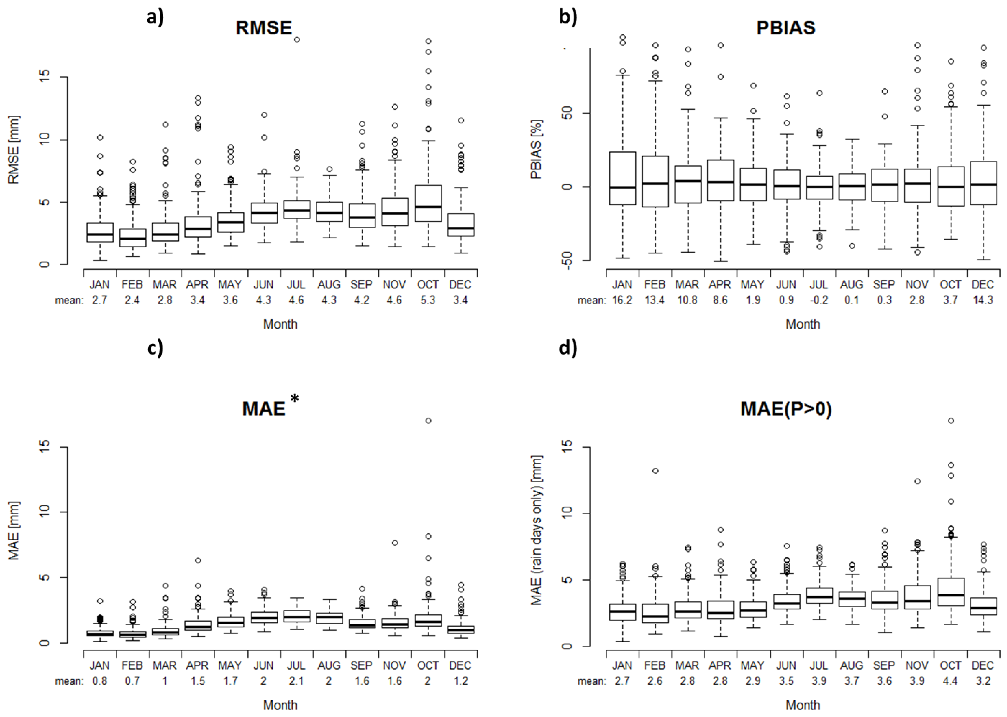
Figure 4 shows the monthly distribution of the four presented criteria. As expected, the course of the RMSE (Figure 4a), MAE* (Figure 4c), and MAE (Figure 4d) followed the distribution of monthly precipitation, with the maximum occurring in the summer and fall months resulting from convective and strong precipitation events. However, the highest spread and overestimation of PBIAS (Figure 4b) was visible for the winter months, which are likely also the months with the highest uncertainty in the observations, due to higher undercatch of snow compared to liquid precipitation [24,25].
3.3. Available Precipitation Data Sets
In the following section, the available precipitation data sets included in this study are briefly introduced. Table 1 gives a short overview over the data sets and their horizontal resolution, as well as the covered time period. The main criteria for the selection of data sets were daily resolution and a temporal coverage, at least for the 20-year period (1989–2008). For this reason, any monthly data sets or daily data sets with a shorter temporal coverage, or a starting date late than 1989, were not included here. The starting and end date were determined to find the maximum overlap for the selected data sets. The horizontal resolution of the included gridded products varied from a 5 km grid to 1° × 1° (~125 km) spacing. Coarser grids, such as the global 20th Century Reanalysis [10] and the NCEP/NCAR Reanalysis [16] data set, were not included due to the relatively small catchment area and the respective coverage of these global data sets. Data sets with a shorter time period available due to a later starting date, such as the Tropical Rainfall Measuring Mission (TRMM) Multisatellite Precipitation Analysis [47], the Climate Prediction Center (CPC) Morphing Technique (CMORPH) [48] and the Global Precipitation Measurement Mission (GPM) [49], were also not included in this study. This led to a selection of eight data sets, as presented in Table 1, which are either interpolated products from station observations, derived from satellite or reanalysis data sets. The data products are shortly introduced in the following, while for detailed information it is referred to the respective publications.
Three observational data sets are included in this study: the Alpine Gridded Data Set (EURO4m-APGD), derived through the EURO4m project [14], the E-OBS data set in version 11 provided through the European Climate Assessment and Dataset (ECA&D), and derived within the ENSEMBLES project [20], as well as the Full Data Daily Product from the Global Precipitation Climatology Centre (GPCC-FDD) provided through the DWD [12]. The EURO4m-APGD was derived from numerous observation stations from various national observatories, and covers the greater Alpine area for the time period 1971–2008. With a 5 km grid size, this data set represents the highest resolution observational data product available for this area so far. The E-OBS data set is widely used in various studies and based on selected observation stations that provide a long data record and ensured quality control. Therefore, less stations are included compared to the EURO4m-APGD [50]; however, the E-OBS data set covers the time period 1951–2015 (and updates are ongoing), with a daily resolution on a 25 km grid over Europe [20]. GPCC-FDD provides precipitation information from station data on a 1.0° grid for the time period 1988–2013. While GPCC offers a multitude of precipitation data sets, the FDD is recommended for daily analysis with focus on extremes and was therefore selected for this study. The GPCC-FDD includes similar stations compared to E-OBS for the interpolation, as indicated by the corresponding variable in the data set.
Four reanalysis products are included in this study, which are available at various resolutions. While most reanalysis data sets assimilate precipitation in some way, are not affected by system changes, temporal and spatial coverage of the observations and undercatch are problematic [51]. The reanalysis data set with the highest horizontal resolution is the MESAN downscaling product on a ~5 km grid. MESAN is derived through the downscaling of HIRLAM 0.2° forecasts, and assimilates observed precipitation from rain gauge data [15]. Additionally, the Modern-Era Retrospective Analysis for Research and Applications, Version 2 (MERRA-2), provided through the National Aeronautics and Space Administration (NASA) which shows considerable improvements over Version 1 [52] with an improved assimilation scheme, was included. In MERRA-2, observed precipitation was used as forcing for the parameterization of the land surface. The data set offers global coverage and starts in 1980, while updates are still ongoing [53], with a horizontal resolution of ~50 km. The two coarsest reanalysis data sets in this study are provided through the European Centre for Medium-Range Weather Forecasts (ECMWF). First, the ERA-Interim global reanalysis at a resolution of approximately 80 km (0.75°) and second, the Reanalysis for the 20th Century (ERA-20C) [54], were chosen. ERA-Interim assimilates various observations from multiple sources in a 12 hr cycle [11], while ERA-20C only assimilates surface and mean sea level pressures and marine winds [55]. Similar to [21] the coarse data sets are not expected to perfectly reproduce the daily precipitation over a complex medium sized catchment. However ERA-Interim is widely used as meteorological forcing for hydrological models in data scarce regions, making this an important data set to include. Especially for the long time period covered, it is also worth including the ERA-20C, since this data set would allow simulations starting in 1900. Additionally, it is interesting to see how this data set, which does not assimilate many observations, performs on the catchment scale.
The only remotely sensed data product included was the bias-corrected version of the multi-satellite Precipitation Estimation from Remotely Sensed Information using Artificial Neural Networks (PERSIANN) specified as PERSIANN-CDR (Climate Data Record). PERSIANN uses infrared brightness temperature derived from geostationary satellite information to estimate the rainfall rate [19]. To reduce the biases in the so-derived precipitation but keep the spatial and temporal patterns at 0.25° resolution, the 2.5° monthly data set by the Global Precipitation Climatology Project (GPCP) [56] is applied for correction.
It is important to note that most data sets are not independent from each other, as most of them include the same station observations directly, or assimilate them in some way. This is however, a common problem in comparison studies, and cannot be avoided.
3.4. Remapping of the Reference Grid
When comparing spatial data sets, a common grid has to be defined to perform the analysis. The highest spatial resolution possible for a comparison is defined by the selected reference grid, and was thus 1 km in this study. This approach however favors higher resolution data sets, as the coarser grids are not able to resolve the fine-scale processes [3]. A second possibility is to perform the comparison at multiple defined resolutions that correspond to meaningful data sets, e.g., the highest resolution and a medium range resolution, as done in some studies [21,50]. Lastly, the comparison can be conducted on the coarser grid, which provides a fair comparison for the coarser grids; however small scale information are lost, which might not be desirable [3].
In this study, a combination of the first and the latter approaches was chosen. A conservative remapping of the reference grid to the resolution of each of the gridded data sets was conducted. The direct evaluation of each data set hence was carried out on the corresponding, coarser grid of each data set. All data sets were then disaggregated to the highest resolution of 1 km to account for the catchment delineations, the number of grid cells, and the correct areal weights for coarser grid cells, where only a small percentage of the grid cell might be within the catchment. Obviously, the coarser data sets had a lower effective resolution, and could not represent the topography at the detailed 1 km resolution. However, there was no additional source of uncertainty introduced through this disaggregation, but rather already captured within the uncertainties of the data sets. Nevertheless, the inter-comparison of the data sets was at a higher resolution and penalized the coarser data sets. This approach was chosen, as the performance should be evaluated on catchment scale with respect to hydrological modeling, which will likely be carried out at even higher resolution.
4. Results
In the following, the results of the comparison are presented, starting with a generic section on the climatological performance of mean precipitation at various time scales. The following subsection then introduces some indicators for a more detailed comparison based on daily precipitation. The uncertainty introduced by elevation only is evaluated in the last section.
4.1. Mean Precipitation
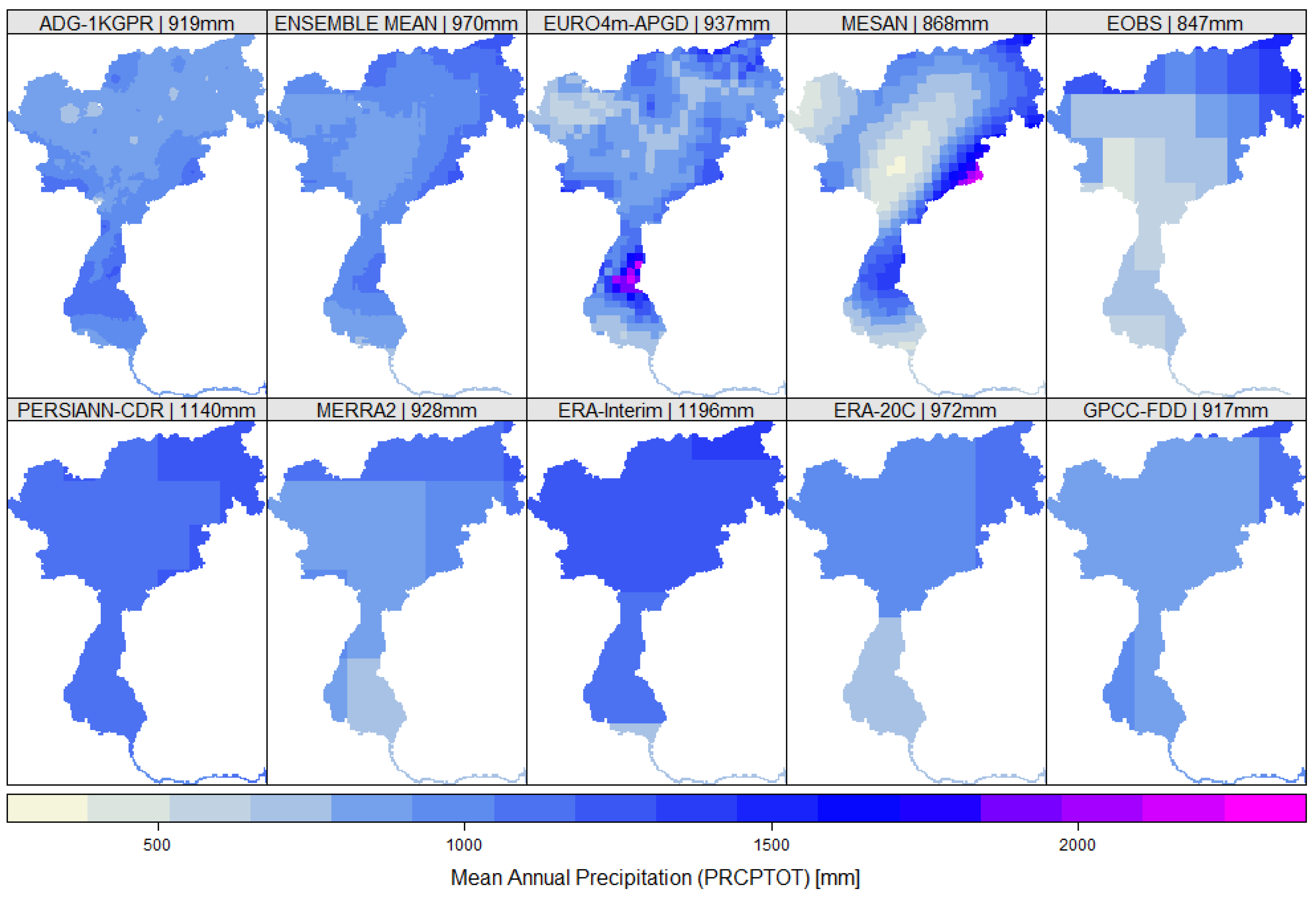
The mean annual precipitation over the Adige catchment for all data sets included in this study is presented in Figure 5, as well as the ensemble mean, derived from all data sets. There was a considerable spread in the catchment mean of 350 mm·y−1 identifiable in the ensemble, corresponding to 35% of the ensemble mean annual precipitation. The highest mean annual precipitation was found in ERA-Interim (1196 mm) and PERSIANN-CDR (1140 mm), while E-OBS (847 mm) and MESAN (868 mm) showed the lowest annual mean precipitation sums. The general inner-alpine dry valleys were present in the high resolution data sets EURO4m-APGD and MESAN, although the extent and the magnitude are overestimated in the latter. These dryer areas were also reproduced by the E-OBS data set; however, there was a strong North-South gradient with lower precipitation in the South. The coarser data sets were not able to reproduce these small scale dry areas, which was not surprising.
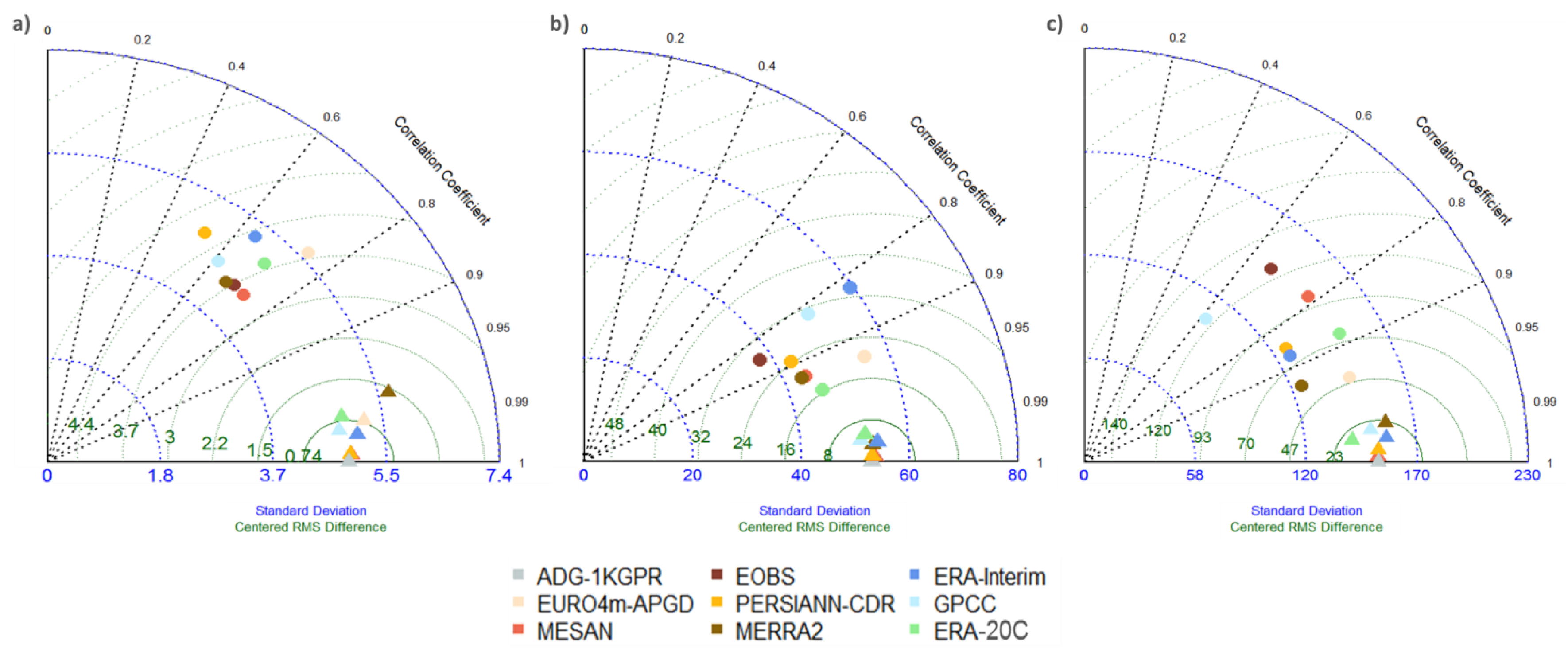
To evaluate the temporal representation and variability of the mean catchment precipitation, Figure 6 shows Taylor diagrams [57] based on daily (a), monthly (b), and annual (c) catchment precipitation of the gridded data sets (circles) and the corresponding aggregated reference grid (triangles) with respect to the reference grid (grey triangle). Dashed lines display the correlation of the evaluated data sets compared to their corresponding reference grid, green arcs the RMSE, and blue, dashed arcs display the standard deviation of each grid. Best agreement, measured by correlation, for both, aggregated reference grids and the evaluated data sets, is given for monthly data. All data sets captured the monthly precipitation reasonably well, with correlation coefficients between 0.8 and 0.95. As expected, daily correlations were considerably lower, with no data set showing correlation greater than 0.8, and overall lower correlations for annual precipitation (with the exception of EURO4m-APGD and MERRA-2). Inter-annual variability, here, simply the standard deviation of the annual precipitation, was represented very well in E-OBS, MESAN, ERA-20C and EURO4m-APGD, while the other data sets underestimated the variability considerably. The ranking for RMSE varied depending on the time scale; however, EURO4m-APGD, MERRA-2 and ERA-20C showed comparatively low errors for all three time scales, while MESAN showed higher errors for annual precipitation. The triangles in the Taylor Diagrams show the effect introduced purely by the spatial resolution and the different grids of the included data sets. They were all derived through aggregation of the ADG-1KGPR to the corresponding coarser grid. As expected, they all showed very high correlations (>0.95) and low RMSE compared to the reference grid at 1 km resolution.
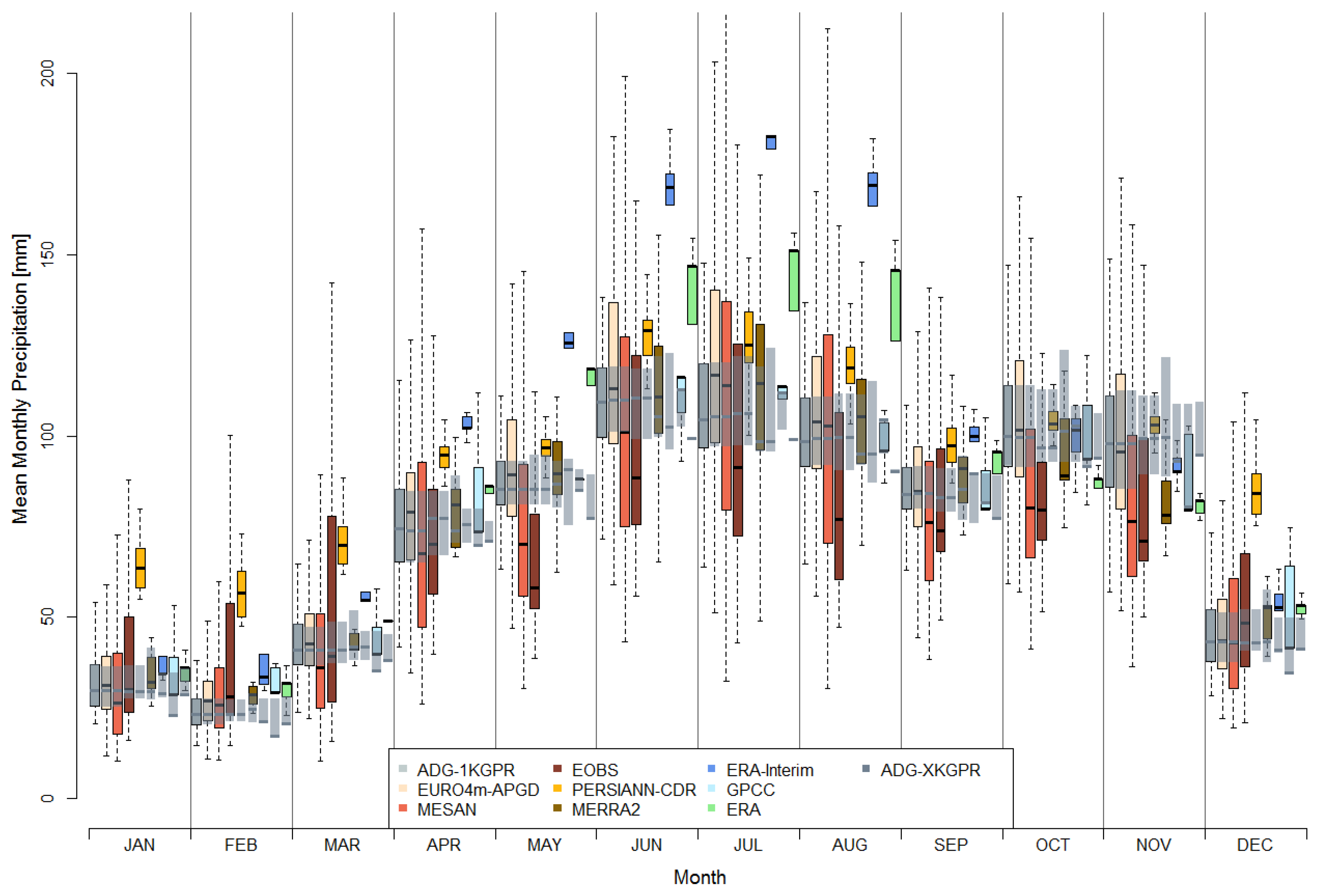
Boxplots for mean monthly precipitation over the catchment are presented in Figure 7. In contrary to Figure 6, the spread within each data set comes from the spatial variability within the long-term monthly mean precipitation over the catchment, derived from grids similar to the annual precipitation sums presented in Figure 5. Darker grey boxplot (first in each month) correspond to the reference grid, colored boxplot to the evaluated data sets and the shaded grey boxplots to each corresponding aggregated reference grid. The latter represent the uncertainty that purely comes from the spatial resolution, as they are conservatively remapped as described in Section 3. Throughout all months, this results in less variability, hence shorter boxplots, with a tendency towards decreasing median precipitation for all months with increasing spatial resolution.
In general, the annual precipitation cycle was captured by all data sets; however, there were distinct differences for the individual data sets and months. The annual cycle was more pronounced in the EMCWF reanalysis products ERA-Interim (dark blue) and ERA-20C (green), and considerably less pronounced in PERSIANN-CDR (yellow). The latter showed an overestimation in winter precipitation of up to 100%. This was caused by the overestimation of precipitation due to cold clouds, where the algorithm for PERSIANN was less accurate [19,28] and was less pronounced in summer. ERA-20C and especially ERA-Interim considerably overestimated summer precipitation, also compared to other reanalysis data sets included in the study. This was important to point out, as precipitation undercatch and the underrepresentation of high-elevation gauges potentially led to an underestimation of precipitation in the observational data sets. Similar to the results presented in Figure 5, E-OBS (dark red) produced a larger spread for monthly precipitation throughout the year, resulting from very high precipitation in the northern, alpine part of the catchment, and very low precipitation in the central and southern parts. This also led to an underestimation of summer precipitation in this data set. All data sets derived from observations agreed for most months, and represent similar magnitudes, which was not too surprising, as they were not independent from each other, and several stations were included in all these data sets. Additionally, the high-resolution data sets better represented the annual cycle and the precipitation magnitudes compared to the other data sets.
The presented differences in monthly precipitation would likely have strong implications for hydrological impact modeling. The presented overestimation in winter for PERSIANN-CDR would likely lead to greater snow pack accumulation, resulting in higher discharge from snow melt in spring. The overestimation in summer in the ERA-Interim and ERA-20C data sets might lead to higher soil moisture in summer, and consequently increased discharge and higher sensitivity to strong precipitation events with respect to flood events.
4.2. Comparison of Hydrologically Important Indicators
To further assess the differences in the data sets, three additional indicators addressing extreme precipitation were derived to estimate the implications for hydrology. These indicators were the maximum number of consecutive days with precipitation <1 mm (CDD, numbers of days), the maximum number of consecutive days with precipitation >1 mm (CWD, numbers of days) [58], and the contribution of heavy precipitation (>95th percentile) to the annual precipitation (R95pTOT, in %) [59]. These were selected, as they provided insights in the performance of the data sets for heavy precipitation, as well as the timing and distribution of precipitation and wet/dry days. All of these indicators are based on daily precipitation.
Figure 8 shows the deviations in CDD for the period 1989–2008 for all selected data sets compared to the corresponding remapped reference grid. The upper panel shows the absolute amount for the reference grid, as well as the ensemble mean. To indicate the spread and the uncertainty within the ensemble, the standard deviation is presented in the top right. This reveals a larger spread, i.e., higher uncertainties, in the central part of the catchment, which is generally characterized by a higher number of consecutive dry days compared to the alpine northern area. The high resolution data sets tend to better represent CDD, whereas the coarser data sets considerably underestimate these. This can be at least partly attributed to the horizontal resolution and smoothed orography, as the aggregated reference grids are based on a 1 km grid and are not interpolated to the respective resolution. The highest underestimation can be found in PERSIANN-CDR (−65 days for the catchment mean), which can be attributed to the less accurate algorithm for cold clouds already mentioned, that overestimates precipitation on cloud covered days especially in winter. The strong underestimation in the ERA-Interim (−32 days) data can not only be attributed to horizontal resolution, as the coarser ERA-20C and GPCC-FDD show a better representation of CDD, but is rather caused by the general overestimation in the frequency of low precipitation days.
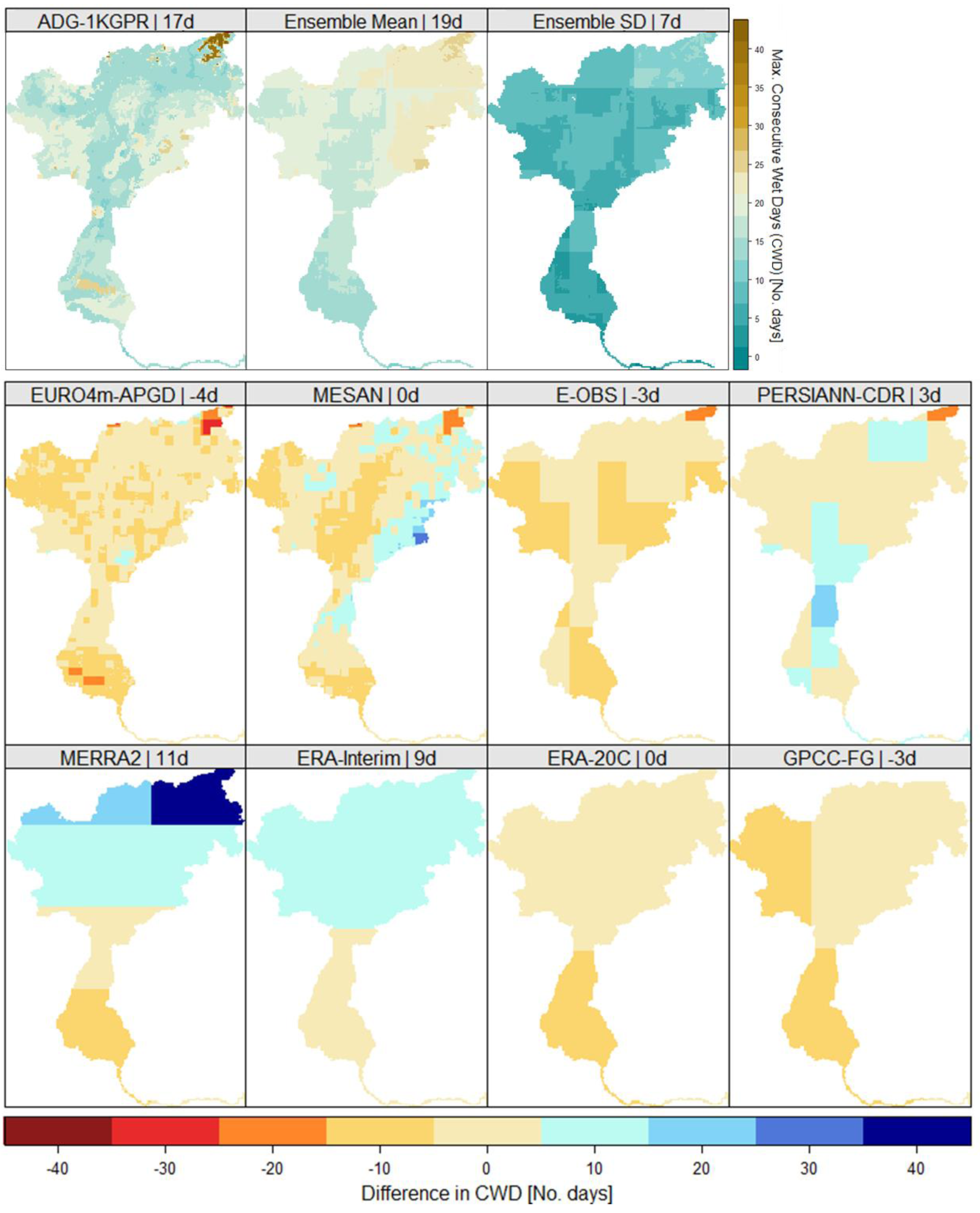
This was confirmed through the maximum number of consecutive wet days (CWD), i.e., days with precipitation >1 mm, presented in Figure 9 in the same way as described for CDD. In general, there is higher agreement throughout the different data sets with the reference grid. The model spread, shown as standard deviation in the top right, was more homogenous than for CDD. Additionally, the data sets agree more, resulting in a smaller spread, i.e., standard deviation of seven compared to 23 days (for CDD). In contrary to CDD, there was no evidence that high resolution data sets perform better, as the coarsest grids, ERA-20C and GPCC-FDD both showed very low deviations from the corresponding reference grid. The highest deviations were found in the MERRA-2 and ERA-Interim reanalysis for the northern part of the catchment through orographic precipitation. These data sets overestimated the mean CWD by 11 days (MERRA-2) and by nine days (ERA-Interim). PERSIANN-CDR also showed a slight overestimation, mostly for the central area of the catchment. However, as for CDD, the data sets derived from observations showed less deviations to the reference data set compared to the reanalysis products, with the exception of the coarse ERA-20C.
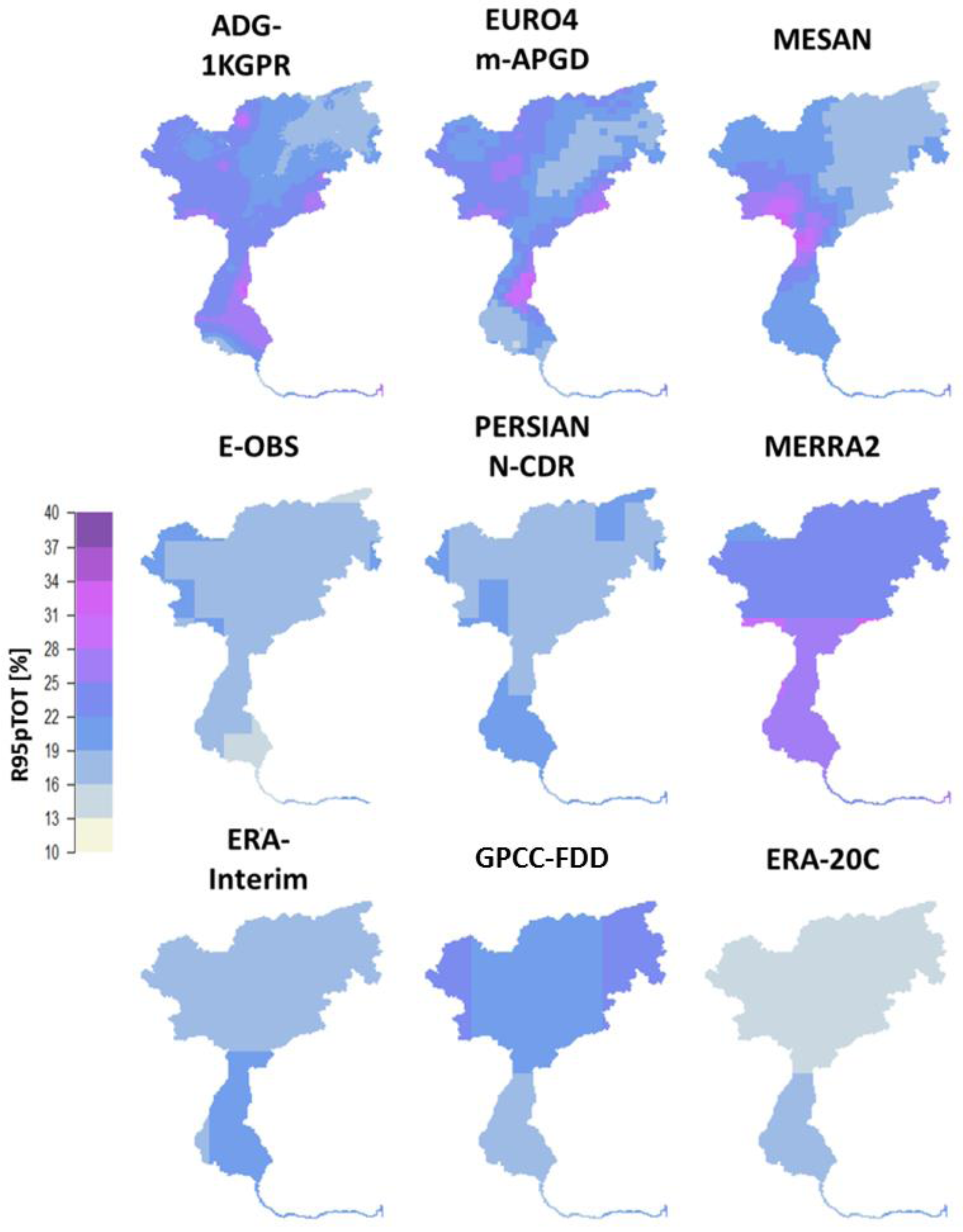
To assess the representation of heavy precipitation events in the data sets, the percent contribution of precipitation from heavy precipitation days, i.e., greater than the 95th percentile, to the total annual precipitation (R95pTOT) is presented in Figure 10. As expected, the coarser data sets tended to reproduce lower values, meaning a lower contribution of heavy precipitation days to the annual precipitation. The high resolution data sets again agreed best with the reference grid, although MESAN showed more homogenous patterns as the EURO4m-APGD and the reference grid, originating from the downscaling of the HIRLAM results. A strong underestimation was present for E-OBS, PERSIANN-CDR, ERA-Interim and ERA-20C. For ERA-Interim there was a known error reported by the ECMWF with the representation of convective events. The convective available potential energy (CAPE) was zero in the data set for the afternoon time steps where most convective events occur. Despite the coarse resolution, MERRA-2 represented the contribution of heavy precipitation well, though it missed out the north-eastern part of the area with a considerably lower share due to the horizontal resolution. In the GPCC data set R95pTOT, the northern part was better reproduced compared to the coarse EMCWF grids; however, the southern part showed lower R95pTOT. This originated from the very low station density in the GPCC-FDD data set in the southern part, with only one station per grid cell, according to the respective variable in the data set.
4.3. Uncertainties and Recommendation
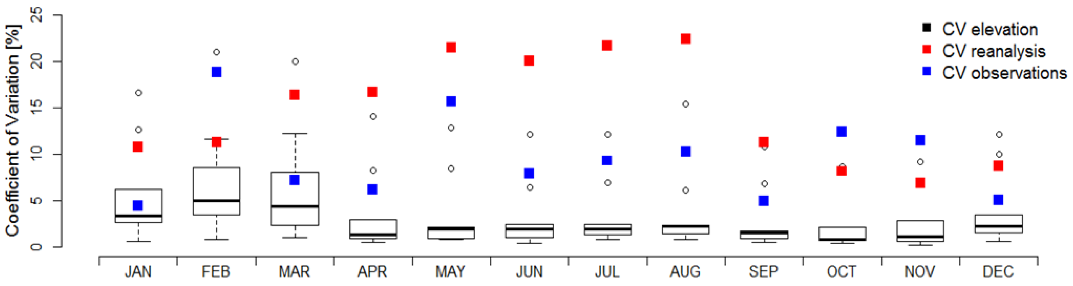
To estimate the relative contribution of spatial resolution compared to the uncertainty introduced by the data sets themselves, the coefficient of variation (CV) is presented. CV is defined as the standard deviation normalized by the mean and given in percent. The data sets were remapped to the corresponding grids of all data sets included and the climatological monthly catchment precipitation was presented at each resolution. These were then compared to the CV derived from the data sets at their native resolution, which were grouped in observational (blue) and reanalysis (red) data sets. PERSIANN-CDR was excluded from this analysis, as it was the only remote sensing data set in the study. Figure 11 shows boxplots for the CV introduced through spatial resolution only, while the red and blue squares correspond to the mean CV in the reanalysis and observation data sets. The CV introduced through elevation only, was derived by remapping each data set to the grids of the other data sets, and calculating CV separately per data set. The variation shown as boxplots hence stems only from the effect of different resolutions and does not include uncertainty through the data sets themselves. The CV shown in red and blue in contrary are based on the variation derived from the data sets at their individual grids, which also includes uncertainty originating from the different resolutions. With the exception of January and March, the uncertainty introduced by the source of the data sets exceeded the contribution of the grid resolution. The relative variability from spatial resolution was higher for the winter months, where the observational data sets also showed greater variability as the reanalysis data sets.
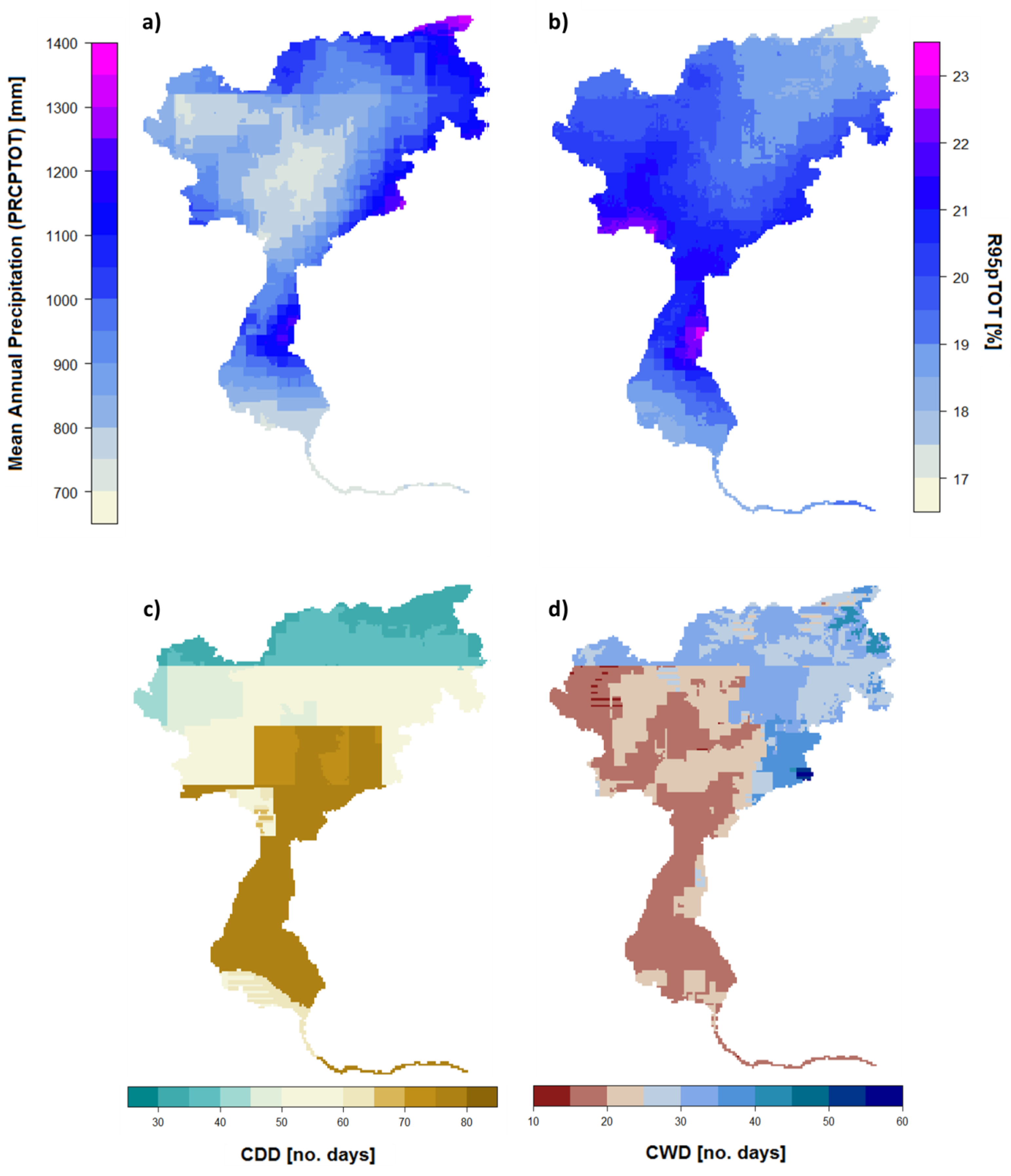
As presented, there was a considerable spread within the available precipitation data sets. To cover most of the uncertainty and benefit from the strength of each selected data set, similar to climate change impact assessment studies, an ensemble approach is recommended to serve as a reference [50]. However, based on the presented indicators, three of the presented data sets were not able to represent the precipitation conditions in the catchment. This conclusion can be drawn based on the comparison to the reference grid, as well as with respect to the other data sets. As also suggested in previous studies [51] the corresponding data set were excluded from the ensemble in this study. This was not done to reduce the overall spread, but rather based on a thorough selection process, as the resulting differences in the data sets were not introduced to different methods or sources of the data sets, but rather bad performance and limited applicability of these data sets over the study area. Therefore, PERSIANN-CDR was excluded, due to the systematic overestimation of precipitation in the winter months, and the considerably underestimation of CDD. Similarly, ERA-Interim and ERA-20C were excluded, as they overestimated summer precipitation and produced too few consecutive dry days and were additionally, due to their coarse resolution, not able to perform well for heavy precipitation (R95pTOT). As the remaining data sets did not show considerable deviations from both the reference and the ensemble mean, they were included to derive the ensemble reference grid presented in Figure 12 for the presented indicators. The mean annual precipitation (Figure 12a) represented small-scale features such as the dry Venosta valley in the north-western part of the catchment, as well as the higher precipitation over the alpine north-eastern part. This was not as pronounced in the reference data set, possibly through low station density, but identifiable in most other gridded data sets. R95pTOT, presented in Figure 12b, follows the patterns of the high resolution data sets, however, with less artifacts introduced through interpolation as for the reference grid, the stations were highly visible in the corresponding R95pTOT. However, the absolute range of R95pTOT was only about two-thirds compared to the reference grid. The maximum number of consecutive dry days (Figure 12c) followed the reference grid; the grid structure of the E-OBS grid was clearly visible, resulting in very sharp and unrealistic boundaries. These were less pronounced for consecutive wet days (Figure 12d) where the higher number of CWD in the north east was dominated by the reanalysis data sets, which showed a higher number of consecutive wet days in this area.
5. Discussion
The presented differences in available precipitation data products highlight the need to take into account the uncertainties related to finding the real reference precipitation. This becomes crucial when data sets are applied to calibrate and validate hydrological models, or are chosen to select a subset or bias correct climate models. Therefore, the uncertainties and differences within the ensemble of available daily, gridded precipitation data products have to be evaluated on the catchment scale. In this study, the uncertainty of gridded precipitation data sets, from various sources and derived through different methods, was investigated over an alpine catchment. It has to be pointed out that findings over this area do not allow for a performance assessment of the presented data sets in general. Whereas the data sets show similar annual precipitation sums and a good representation of the inter-annual variability, i.e., standard deviation, they show clear differences on daily time scale. Although all data sets capture the annual cycle of precipitation, they show large differences in the magnitudes, up to 100% in some months for mean catchment precipitation. This confirms the results presented by previous studies over Europe [50] and the alpine region [21] also on a catchment scale. This study confirms the limitations of the satellite precipitation product PERSIANN-CDR, which led to a systematic overestimation of precipitation, especially in winter, likely due to non-raining clouds where the algorithm performs worse than for e.g., warm tropical convective systems [19]. This overestimation, especially in winter was, also identified over most of Europe in general [50]. Increased precipitation in winter will likely result in a larger snow pack that will influence the peaks in discharge for the spring months, due to snow melt. The slight overestimation of summer precipitation by PERSIANN-CDR confirms recent findings for the PERSIANN data product with respect to convective events and better agreement in fall, where precipitation is dominated by stratiform systems [32]. However, the bias-corrected CDR applied in this study improved the PERSIANN data set considerably, as the overestimation was not as pronounced in this study over the same region. Clear outliers in the summer months were the two reanalysis data sets from EMCWF, especially ERA-Interim, which confirms the findings in the studies mentioned. Similar to the results presented for the comparison with station data [60], there is a higher agreement between reanalysis data sets and observational data sets in winter. This can be confirmed also by the lower coefficients of variation in the winter months for both groups of data sets. Differences in the performance of the observational data sets is strongly linked to station density [2], which is extremely low in the E-OBS data set [21] and, especially for the southern part of the catchment, also for GPCC-FDD. This leads to underestimated precipitation for E-OBS in annual, as well as seasonal (summer), precipitation and an increased number of consecutive dry days for the southern parts.
One source of uncertainty in the different data sets is the spatial resolution. As expected, the high resolution data sets generally better represent the regional or local patterns for both mean precipitation, as well as for several indicators such as consecutive dry and wet days, and the contribution of heavy precipitation to the annual precipitation. Nevertheless, this is not dependent on the source of the data set, as higher resolution reanalysis show similar patterns to the reference grid, such as dry areas and areas where heavy precipitation has a higher share in the annual precipitation. However, the reanalysis data sets included in this study show less consecutive dry days and more consecutive wet days compared to the observational data sets. To evaluate the effect of different resolutions on the model spread, the coefficient of variation was selected to estimate the relative contribution of the spatial resolution. The spread originating from spatial resolution is considerably lower, and generally dominated by the model spread. This is crucial, as it highlights the applicability also of coarser data sets on the catchment scale, assuming that the data set is able to represent the general precipitation features of the area.
As this study focusses on the applicability of gridded precipitation products as meteorological input for hydrological models, it is important to assess not only their climatology, but also evaluate their performance on daily time steps. Therefore, three indicators were presented, focusing on potential impacts on low and high flows, as well as the occurrence of high precipitation events. The results presented in this study indicated strong differences in the number of consecutive dry (CDD) and wet days (CWD), and the contribution of heavy precipitation to the annual precipitation (R95pTOT). For the reanalysis data sets, the results highlight a higher contribution of low but steady precipitation events resulting in a lower R95pTOT, more CWD, and less CDD. These precipitation characteristics highly impact potential hydrological modeling, as steady moderate rainfall events infiltrates in the soil and will be available for plants, whereas higher intensity events of the same total amount might lead to flooding, and to eventually lower soil moistures [61]. Additionally, there is a higher sensitivity of flood response to temporal than spatial variability [8]. The sensitivity for discharge response to the spatial resolution of the rainfall event over smaller catchments is low, and the impact only moderate over large catchments [62]. The differences in the length of the dry spells is particularly important for low flows [63] which are of interest, especially for the southern part of the Adige catchment, and the agricultural areas that are characterized by irrigation, and affected by seasonal water scarcity [37].
As observational data sets are prone to undercatch and measurement errors, which are amplified in winter [24,25], and the location and density of precipitation stations [21] it is obvious that these data sets have large uncertainties, especially in the higher elevations where station density is low, or no stations are present at all. To bridge this gap, (regional) reanalysis data sets show great potential [50], and should therefore be included in the analysis to find the best possible reference precipitation. Although the remote sensing data set did not perform acceptably over this catchment, it is still important not to neglect these data sets and include them in the selection process. Similar to climate impact assessment studies and confirming recent findings [50], an ensemble approach is presented and recommended in this study to derive a more robust precipitation data set. This will help to overcome the issues with observations, especially over complex topography, and to quantify and reduce the related uncertainties. Nevertheless, the recent study highlights the importance of detecting data sets that show high deviations on the catchment scale, and exclude them from the ensemble. This is not proposed to reduce the ensemble spread, but rather is based on a careful selection process. As presented, a variety of indicators should be evaluated, and selected specifically for the desired application, to identify data sets that are not capable of reproducing the given conditions in a specific area or catchment. The data sets excluded from the ensemble all showed clear mismatches with not only the reference grid, but also the rest of the ensemble, and could therefore be excluded from the ensemble. Additionally, a more dense station network is required, also in the higher elevations, to reduce the uncertainties in the observational data sets. This is especially crucial for the alpine areas in the northern parts of the catchment that are characterized by complex topography. It must be highlighted, that the selection of data sets is highly dependent on the region and hardly transferable to other regions and climate zones. The final ensemble mean now provides a robust basis for further activities such as hydrological modeling, climate model selection, and potentially for bias correction of climate model data.
Acknowledgments
This work has been supported by the European Communities 7th Framework Programme Funding under Grant agreement no. 603629-ENV-2013-6.2.1-Globaqua.
Author Contributions
The study was carried out by the first author as part of his PhD research, supervised by the second author. Both authors contributed to the concept and writing of this paper, with the first author preparing the first version of the manuscript.
Conflicts of Interest
The authors declare no conflict of interest. The founding sponsors had no role in the design of the study; in the collection, analyses, or interpretation of data; in the writing of the manuscript, and in the decision to publish the results.
References
- Schneider, U.; Ziese, M.; Meyer-Christoffer, A.; Finger, P.; Rustemeier, E.; Becker, A. The new portfolio of global precipitation data products of the Global Precipitation Climatology Centre suitable to assess and quantify the global water cycle and resources. Proc. Int. Assoc. Hydrol. Sci. 2016, 374, 29. [Google Scholar] [CrossRef]
- Daly, C.; Slater, M.E.; Roberti, J.A.; Laseter, S.H.; Swift, L.W. High-resolution precipitation mapping in a mountainous watershed: Ground truth for evaluating uncertainty in a national precipitation dataset. Int. J. Climatol. 2017, 37, 124–137. [Google Scholar] [CrossRef]
- Prein, A.F.; Gobiet, A.; Truhetz, H.; Keuler, K.; Goergen, K.; Teichmann, C.; Fox Maule, C.; van Mejgaard, E.; Déqué, M.; Nikulin, G.; et al. Precipitation in the EURO-CORDEX 0.11° and 0.44° simulations: High resolution, high benefits? Clim. Dyn. 2016, 46, 383–412. [Google Scholar] [CrossRef] [Green Version]
- Ivancic, T.J.; Shaw, S.B. Examining why trends in very heavy precipitation should not be mistaken for trends in very high river discharge. Clim. Chang. 2015, 133, 681–693. [Google Scholar] [CrossRef]
- Stephens, E.; Day, J.J.; Pappenberger, F.; Cloke, H. Precipitation and floodiness. Geophys. Res. Lett. 2015, 42, 316–323. [Google Scholar] [CrossRef]
- Madsen, H.; Lawrence, D.; Lang, M.; Martinkova, M.; Kjeldsen, T.R. Review of trend analysis and climate change projections of extreme precipitation and floods in Europe. J. Hydrol. 2015, 519, 3634–3650. [Google Scholar] [CrossRef] [Green Version]
- Bacchi, B.; Kottegoda, N.T. Identification and calibration of spatial correlation patterns of rainfall. J. Hydrol. 1995, 165, 311–348. [Google Scholar] [CrossRef]
- Paschalis, A.; Fatichi, S.; Molnar, P.; Rimkus, S.; Burlando, P. On the effects of small scale space–time variability of rainfall on basin flood response. J. Hydrol. 2014, 514, 313–327. [Google Scholar] [CrossRef]
- Hijmans, R.J.; Cameron, S.E.; Parra, J.L.; Jones, P.G.; Jarvis, A. Very high resolution interpolated climate surfaces for global land areas. Int. J. Climatol. 2005, 25, 1965–1978. [Google Scholar] [CrossRef]
- Compo, G.P.; Whitaker, J.S.; Sardeshmukh, P.D.; Matsui, N.; Allan, R.J.; Yin, X.; Gleason, E., Jr.; Vose, R.S.; Rutledge, G.; Bessemoulin, P.; et al. The twentieth century reanalysis project. Q. J. R. Meteorol. Soc. 2011, 137, 1–28. [Google Scholar] [CrossRef]
- Dee, D.; Uppala, S.M.; Simmons, A.J.; Berrisford, P.; Poli, P.; Kobayashi, S.; Andrae, U.; Balmaseda, M.A.; Balsamo, G.; Bauer, P.; et al. The ERA-Interim reanalysis: Configuration and performance of the data assimilation system. Q. J. R. Meteorol. Soc. 2011, 137, 553–597. [Google Scholar] [CrossRef]
- Schamm, K.; Ziese, M.; Raykova, K.; Becker, A.; Finger, P.; Meyer-Christoffer, A.; Schneider, U. GPCC Full Data Daily Version 1.0: Daily Land-Surface Precipitation from Rain Gauges Built on GTS Based and Historic Data. Available online: https://rda.ucar.edu/datasets/ds497.0/ (accessed on 30 July 2017).
- Herrera, S.; Gutiérrez, J.M.; Ancell, R.; Pons, M.R.; Frías, M.D.; Fernández, J. Development and analysis of a 50-year high-resolution daily gridded precipitation dataset over Spain (Spain02). Int. J. Climatol. 2012, 32, 74–85. [Google Scholar] [CrossRef] [Green Version]
- Isotta, F.A.; Frei, C.; Weilguni, V.; Percec Tadic, M.; Lassègues, P.; Rudolf, B.; Pavan, V.; Cacciamani, C.; Antolini, G.; Ratto, S.M.; et al. The climate of daily precipitation in the Alps: Development and analysis of a high-resolution grid dataset from pan-Alpine rain-gauge data. Int. J. Climatol. 2014, 34, 1657–1675. [Google Scholar] [CrossRef]
- Häggmark, L.; Ivarsson, I.; Gollvik, S.; Olofsson, O. Mesan, an operational mesoscale analysis system. Tellus 2000, 52, 2–20. [Google Scholar] [CrossRef]
- Kalnay, E.; Kanamitsu, M.; Kistler, R.; Collins, W.; Deaven, D.; Gandin, L.; Iredell, M.; Saha, S.; White, G.; Woollen, J.; et al. The NCEP/NCAR 40-year reanalysis project. Bull. Am. Meteorol. Soc. 1996, 77, 437–471. [Google Scholar] [CrossRef]
- Rienecker, M.M.; Suarez, M.J.; Gelaro, R.; Todling, R.; Bacmeister, J.; Liu, E.; Bosilovich, M.G.; Schubert, S.D.; Takacs, L.; Kim, G.-K.; et al. MERRA: NASA’s modern-era retrospective analysis for research and applications. J. Clim. 2011, 24, 3624–3648. [Google Scholar] [CrossRef]
- Kummerow, C.; Barnes, W.; Kozu, T.; Shiue, J.; Simpson, J. The tropical rainfall measuring mission (TRMM) sensor package. J. Atmos. Ocean. Technol. 1998, 15, 809–817. [Google Scholar] [CrossRef]
- Ashouri, H.; Hsu, K.L.; Sorooshian, S.; Braithwaite, D.K.; Knapp, K.R.; Cecil, L.D.; Nelson, B.R.; Prat, O.P. PERSIANN-CDR: Daily precipitation climate data record from multisatellite observations for hydrological and climate studies. Bull. Am. Meteorol. Soc. 2015, 96, 69. [Google Scholar] [CrossRef]
- Haylock, M.R.; Hofstra, N.; Klein Tank, A.M.G.; Klok, E.J.; Jones, P.D.; New, M. A European daily high resolution gridded data set of surface temperature and precipitation for 1950–2006. J. Geophys. Res. 2008, 113, D20. [Google Scholar] [CrossRef]
- Isotta, F.A.; Vogel, R.; Frei, C. Evaluation of European regional reanalyses and downscalings for precipitation in the Alpine region. Meteorologische Zeitschrift 2015, 24, 15–37. [Google Scholar] [CrossRef]
- Beck, H.E.; van Dijk, A.I.J.M.; Levizzani, V.; Schellekens, J.; Miralles, D.G.; Martens, B.; de Roo, A. MSWEP: 3-h 0.25° global gridded precipitation (1979–2015) by merging gauge, satellite, and reanalysis data. Hydrol. Earth Syst. Sci. 2017, 21, 589–615. [Google Scholar] [CrossRef]
- Blenkinsop, S.; Lewsis, E.; Chan, S.C.; Fowler, H.J. Quality-control of an hourly rainfall dataset and climatology of extremes for the UK. Int. J. Climatol. 2016, 37, 722–740. [Google Scholar] [CrossRef] [PubMed]
- Goodison, B.E.; Louie, P.Y.T.; Yang, D. WMO Solid Precipitation Measurement Intercomparison; Final Report, WMO/TD-No. 872; World Meteorological Organization: Geneva, Switzerland, 1998. [Google Scholar]
- Rasmussen, R.; Baker, B.; Kochendorfer, J.; Meyers, T.; Landolt, S.; Fischer, A.P.; Black, J.; Thériault, J.M.; Kucera, P.; Gochis, D.; et al. How well are we measuring snow: The NOAA/FAA/NCAR winter precipitation test bed. Bull. Am. Meteorol. Soc. 2012, 93, 811–829. [Google Scholar] [CrossRef]
- Kotlarski, S.; Keuler, K.; Christensen, O.B.; Colette, A.; Déqué, M.; Gobiet, A.; Goergen, K.; Jacob, D.; Lüthi, D.; van Meijgaard, E.; et al. Regional climate modeling on European scales: A joint standard evaluation of the EURO-CORDEX RCM ensemble. Geosci. Model. Dev. 2014, 7, 1297–1333. [Google Scholar] [CrossRef]
- Bosilovich, M.G.; Chen, J.; Robertson, F.R.; Adler, R.F. Evaluation of global precipitation in reanalyses. J. Appl. Meteorol. Climatol. 2008, 47, 2279–2299. [Google Scholar] [CrossRef]
- Kidd, C.; Bauer, P.; Turk, J.; Huffman, G.J.; Joyce, R.; Hsu, K.L.; Braithwaite, D. Intercomparison of high-resolution precipitation products over Northwest Europe. J. Hydrometeorol. 2012, 13, 67–83. [Google Scholar] [CrossRef]
- Nkiaka, E.; Nawaz, N.R.; Lovett, J.C. Evaluating global reanalysis precipitation datasets with rain gauge measurements in the Sudano-Sahel region: Case study of the Logone catchment, Lake Chad Basin. Meteorol. Appl. 2017, 24, 9–18. [Google Scholar] [CrossRef]
- Palazzi, E.; Hardenberg, J.; Provenzale, A. Precipitation in the Hindu-Kush Karakoram Himalaya: Observations and future scenarios. J. Geophys. Res. Atmos. 2013, 118, 85–100. [Google Scholar] [CrossRef]
- Sikorska, A.E.; Seibert, J. Value of different precipitation data for flood prediction in an alpine catchment: A Bayesian approach. J. Hydrol. 2016. [Google Scholar] [CrossRef]
- Maggioni, V.; Nikolopoulos, E.I.; Anagnostou, E.N.; Borga, M. Modeling satellite precipitation errors over mountainous terrain: The influence of gauge density, seasonality, and temporal resolution. IEEE Trans. Geosci. Remote Sens. 2017, 55, 4130–4140. [Google Scholar] [CrossRef]
- Mei, Y.; Anagnostou, E.N.; Nikolopoulos, E.I.; Borga, M. Error analysis of satellite precipitation products in mountainous basins. J. Hydrometeorol. 2014, 15, 1778–1793. [Google Scholar] [CrossRef]
- Nikolopoulos, E.I.; Anagnostou, E.N.; Borga, M. Using high-resolution satellite rainfall products to simulate a major flash flood event in northern Italy. J. Hydrometeorol. 2013, 14, 171–185. [Google Scholar] [CrossRef]
- Frei, C.; Schär, C. A precipitation climatology of the Alps from high-resolution rain-gauge observations. Int. J. Climatol. 1998, 18, 873–900. [Google Scholar] [CrossRef]
- Chiogna, G.; Majone, B.; Cano Paoli, K.; Diamantini, E.; Stella, E.; Mallucci, S.; Lencioni, V.; Zandonai, F.; Bellin, A. A review of hydrological and chemical stressors in the Adige catchment and its ecological status. Sci. Total Environ. 2016, 540, 429–443. [Google Scholar] [CrossRef] [PubMed]
- Navarro-Ortega, A.; Acuña, V.; Bellin, A.; Burek, P.; Cassiani, G.; Choukr-Allah, R.; Dolédec, S.; Elosegi, A.; Ferrari, F.; Ginebreda, A.; et al. Managing the effects of multiple stressors on aquatic ecosystems under water scarcity. The GLOBAQUA project. Sci. Total Environ. 2015, 503, 3–9. [Google Scholar] [CrossRef] [PubMed]
- Schulla, J.; Jasper, K. Model Description Wasim-Eth; Technical Report; Institute for Atmospheric and Climate Science, Swiss Federal Institute of Technology: Zürich, Switzerland, 2007. [Google Scholar]
- Camera, C.; Bruggeman, A.; Hadjinicolaou, P.; Pashiardis, S.; Lange, M.A. Evaluation of interpolation techniques for the creation of gridded daily precipitation (1 × 1 km2); Cyprus, 1980–2010. J. Geophys. Res. Atmos. 2014, 119, 693–712. [Google Scholar] [CrossRef]
- Di Luzio, M.; Johnson, G.; Daly, C.; Eischeid, J.K.; Arnold, J. Constructing retrospective gridded daily precipitation and temperature datasets for the conterminous united states. Am. Meteorol. Soc. 2008, 47, 475–497. [Google Scholar] [CrossRef]
- Lu, G.Y.; Wong, D.W. An adaptive inverse-distance weighting spatial interpolation technique. Comput. Geosci. 2008, 34, 1044–1055. [Google Scholar] [CrossRef]
- Hasenauer, H.; Merganicova, K.; Petritsch, R.; Pietsch, S.A.; Thornton, P.E. Validating daily climate interpolations over complex terrain in Austria. Agric. For. Meteorol. 2003, 119, 87–107. [Google Scholar] [CrossRef]
- Chai, T.; Draxler, R.R. Root mean square error (RMSE) or mean absolute error (MAE)?—Arguments against avoiding RMSE in the literature. Geosci. Model. Dev. 2014, 7, 1247–1250. [Google Scholar] [CrossRef]
- Hutchinson, M.F.; McKenney, D.W.; Lawrence, K.; Pedlar, J.H.; Hopkinson, R.F.; Milewska, E.; Papadopol, P. Development and testing of Canada-wide interpolated spatial models of daily minimum–maximum temperature and precipitation for 1961–2003. Am. Meteorol. Soc. 2009, 48, 725–741. [Google Scholar] [CrossRef]
- Hunter, R.D.; Meentemeyer, R.K. Climatologically aided mapping of daily precipitation and temperature. J. Appl. Meteorol. 2005, 44, 1501–1510. [Google Scholar] [CrossRef]
- Xia, Y.; Fabian, P.; Winterhalter, M.; Zhao, M. Forest climatology: Estimation and use of daily climatological data for Bavaria, Germany. Agric. For. Meteorol. 2001, 106, 87–103. [Google Scholar] [CrossRef]
- Huffman, G.J.; Adler, R.F.; Bolvin, D.T.; Gu, G.; Nelkin, E.J.; Bowman, K.P.; Hong, Y.; Stocker, E.F.; Wolff, D.B. The TRMM Multisatellite Precipitation Analysis (TMPA): Quasi-global, multi-year, combined-sensor precipitation estimates at fine scales. J. Hydrometeorol. 2007, 8, 38–55. [Google Scholar] [CrossRef]
- Joyce, R.J.; Janowiak, J.E.; Arkin, P.A.; Xie, P. CMORPH: A method that produces global precipitation estimates from passive microwave and infrared data at high spatial and temporal resolution. J. Hydrometeorol. 2004, 5, 487–503. [Google Scholar] [CrossRef]
- Hou, A.Y.; Kakar, R.K.; Neeck, S.; Azarbarzin, A.A.; Kummerow, C.D.; Kojima, M.; Oki, R.; Nakamura, K.; Iguchi, T. The global precipitation measurement mission. Bull. Am. Meteorol. Soc. 2014, 95, 701–722. [Google Scholar] [CrossRef]
- Prein, A.; Gobiet, A. Impacts of uncertainties in European gridded precipitation observations on regional climate analysis. Int. J. Climatol. 2017, 37, 305–327. [Google Scholar] [CrossRef] [PubMed]
- Ma, L.; Zhang, T.; Frauenfeld, O.W.; Ye, B.; Yang, D.; Qin, D. Evaluation of precipitation from the ERA-40, NCEP-1, and NCEP-2 Reanalyses and CMAP-1, CMAP-2, and GPCP-2 with ground-based measurements in China. J. Geophys. Res. 2009, 114, D9. [Google Scholar] [CrossRef]
- Reichle, R.H.; Liu, Q.; Koster, R.D.; Draper, C.S.; Mahanama, S.P.; Partyka, G.S. Land surface precipitation in MERRA-2. J. Clim. 2017, 30, 1642–1664. [Google Scholar] [CrossRef]
- Bosilovich, M.G.; Lucchesi, R.; Suarez, M. MERRA-2: File Specification; GMAO Office Note No. 9 (Version 1.1). 2015; 73p. Available online: https://gmao.gsfc.nasa.gov/pubs/ (accessed on 30 November 2017).
- Poli, P.; Hersbach, H.; Dee, D.P.; Berrisford, P.; Simmons, A.J.; Vitart, F.; Trémolet, Y. ERA-20C: An atmospheric reanalysis of the twentieth century. J. Clim. 2016, 29, 4083–4097. [Google Scholar] [CrossRef]
- Hersbach, H.; Poli, P.; Dee, D. The observation feedback archive for the ICOADS and ISPD data sets. ERA Rep. Ser. 2015, 18, 74–85. [Google Scholar]
- Adler, R.F.; Huffman, G.J.; Chang, A.; Ferraro, R.; Xie, P.P.; Janowiak, J.; Rudolf, B.; Schneider, U.; Curtis, S.; Bolvin, D.; et al. The version-2 global precipitation climatology project (GPCP) monthly precipitation analysis (1979–present). J. Hydrometeorol. 2003, 4, 1147–1167. [Google Scholar] [CrossRef]
- Taylor, K.E. Summarizing multiple aspects of model performance in a single diagram. J. Geophys. Res. 2001, 106, 7183–7192. [Google Scholar] [CrossRef]
- Frich, P.; Alexander, L.V.; Della-Marta, P.; Gleason, B.; Haylock, M.; Klein, A.G.; Peterson, T. Observed coherent changes in climate extremes during the second half of the twentieth century. Clim. Res. 2002, 19, 193–212. [Google Scholar] [CrossRef]
- Kioutsioukis, I.; Melas, D.; Zerefos, C. Statistical assessment of changes in climate extremes over Greece (1955–2002). Int. J. Climatol. 2010, 30, 1723–1737. [Google Scholar] [CrossRef]
- Zolina, O.; Kapala, A.; Simmer, C.; Gulev, S.K. Analysis of extreme precipitation over Europe from different reanalyses: A comparative assessment. Glob. Planet. Chang. 2004, 44, 129–161. [Google Scholar] [CrossRef]
- Trenberth, K.E. The impact of climate change and variability on heavy precipitation, floods, and droughts. Encycl. Hydrol. Sci. 2008, 17. [Google Scholar] [CrossRef]
- Nicótina, L.; Alessi Celegon, E.; Rinaldo, A.; Marani, M. On the impact of rainfall patterns on the hydrologic response. Water Resour. Res. 2008, 44. [Google Scholar] [CrossRef]
- Diaz-Nieto, J.; Wilby, R.L. A comparison of statistical downscaling and climate change factor methods: Impacts on low flows in the River Thames, United Kingdom. Clim. Chang. 2005, 69, 245–268. [Google Scholar] [CrossRef]
Figure 1.
Location of the Adige catchment and corresponding elevation.
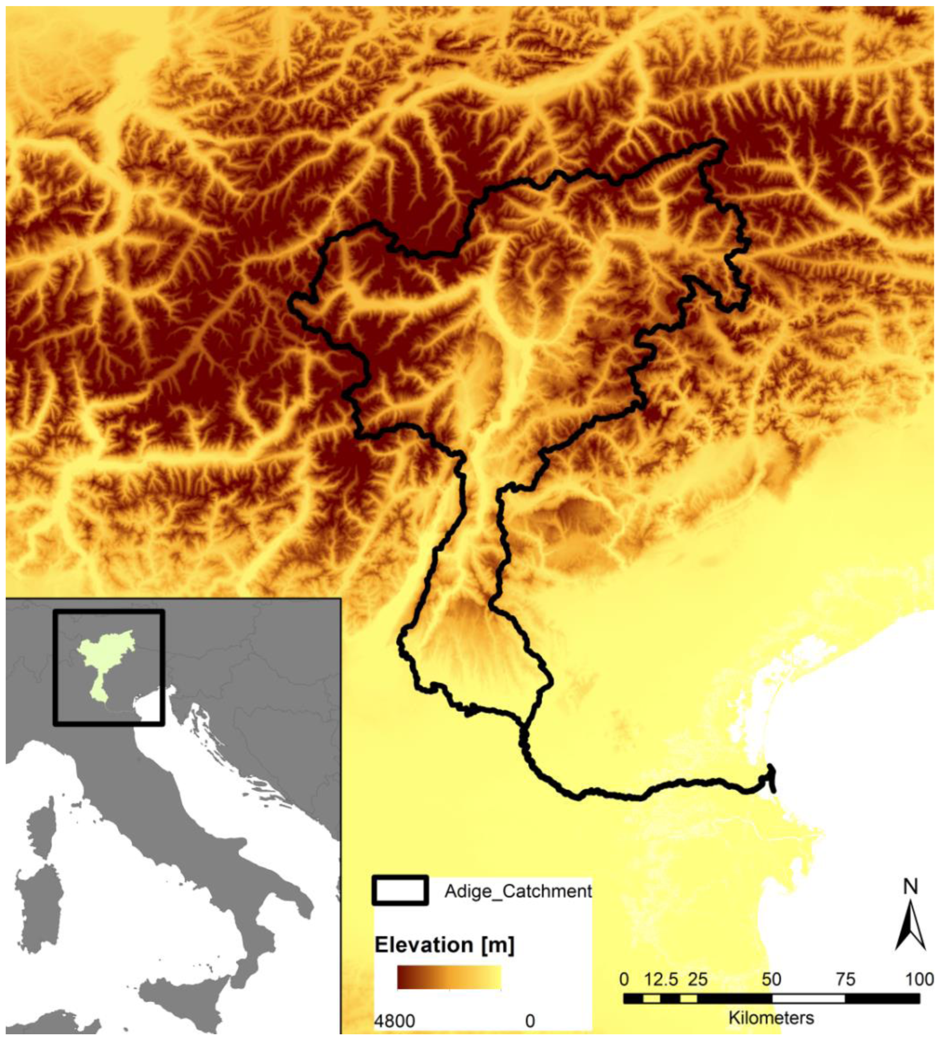
Figure 2.
Mean annual precipitation sums for the observation stations.

Figure 3.
Evaluation of interpolation performance at various precipitation stations over the Adige catchment. Assessment through the indicators: MAE* (a); Mean Absolute Error (MAE) (b) and Root Mean Square Error (RMSE) (c); and Percent Bias (PBIAS) (d). Stations outside the catchment are masked.
Figure 3.
Evaluation of interpolation performance at various precipitation stations over the Adige catchment. Assessment through the indicators: MAE* (a); Mean Absolute Error (MAE) (b) and Root Mean Square Error (RMSE) (c); and Percent Bias (PBIAS) (d). Stations outside the catchment are masked.
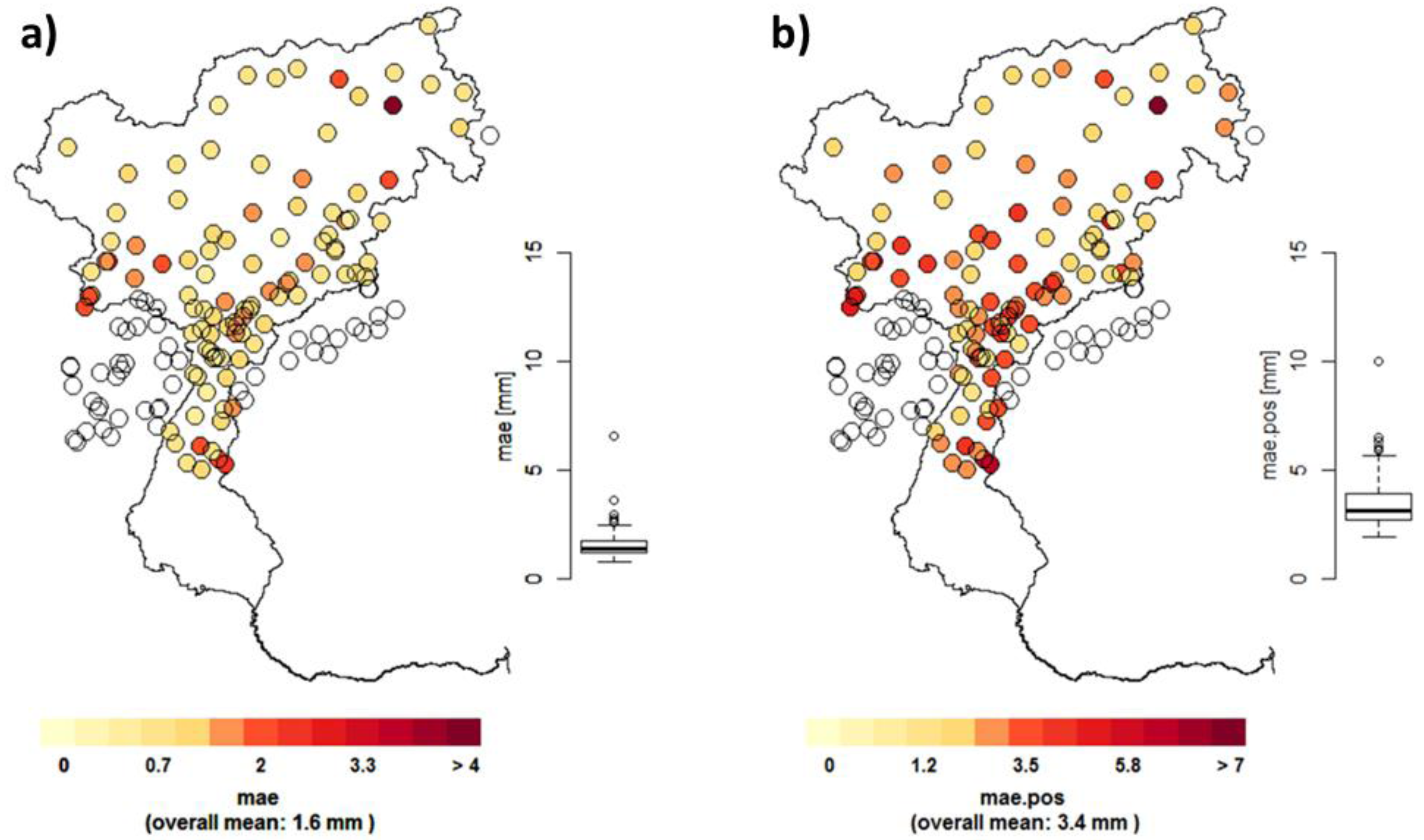

Figure 4.
Evaluation of interpolation performance at monthly scale, boxplots result from mean results at each observation station over the Adige catchment. Four indicators presented: RMSE (a); PBIAS (b); MAE* (c); and MAE (d).
Figure 4.
Evaluation of interpolation performance at monthly scale, boxplots result from mean results at each observation station over the Adige catchment. Four indicators presented: RMSE (a); PBIAS (b); MAE* (c); and MAE (d).

Figure 5.
Mean annual precipitation over the catchment for the applied data sets including the ensemble mean; numbers in the panels correspond to the mean catchment precipitation.
Figure 5.
Mean annual precipitation over the catchment for the applied data sets including the ensemble mean; numbers in the panels correspond to the mean catchment precipitation.

Figure 6.
Taylor Diagram based on daily (a); monthly (b) and annual (c) catchment mean precipitation for the Adige catchment. Circles correspond to the gridded precipitation data sets, while triangles refer to aggregated reference grid.
Figure 6.
Taylor Diagram based on daily (a); monthly (b) and annual (c) catchment mean precipitation for the Adige catchment. Circles correspond to the gridded precipitation data sets, while triangles refer to aggregated reference grid.

Figure 7.
Monthly Precipitation Sums for the applied data sets. The grey boxplots correspond to the high resolution Water Flow and Balance Simulation Model (WaSiM) aggregation, while shaded boxes show the boxplots for the respective grids.
Figure 7.
Monthly Precipitation Sums for the applied data sets. The grey boxplots correspond to the high resolution Water Flow and Balance Simulation Model (WaSiM) aggregation, while shaded boxes show the boxplots for the respective grids.

Figure 8.
Maximum number of consecutive dry days (CDD) in ADG-1KGPR, the ensemble mean and corresponding standard deviation (top row) and the deviations from the corresponding reference grid for the eight gridded data sets (middle & bottom row).
Figure 8.
Maximum number of consecutive dry days (CDD) in ADG-1KGPR, the ensemble mean and corresponding standard deviation (top row) and the deviations from the corresponding reference grid for the eight gridded data sets (middle & bottom row).
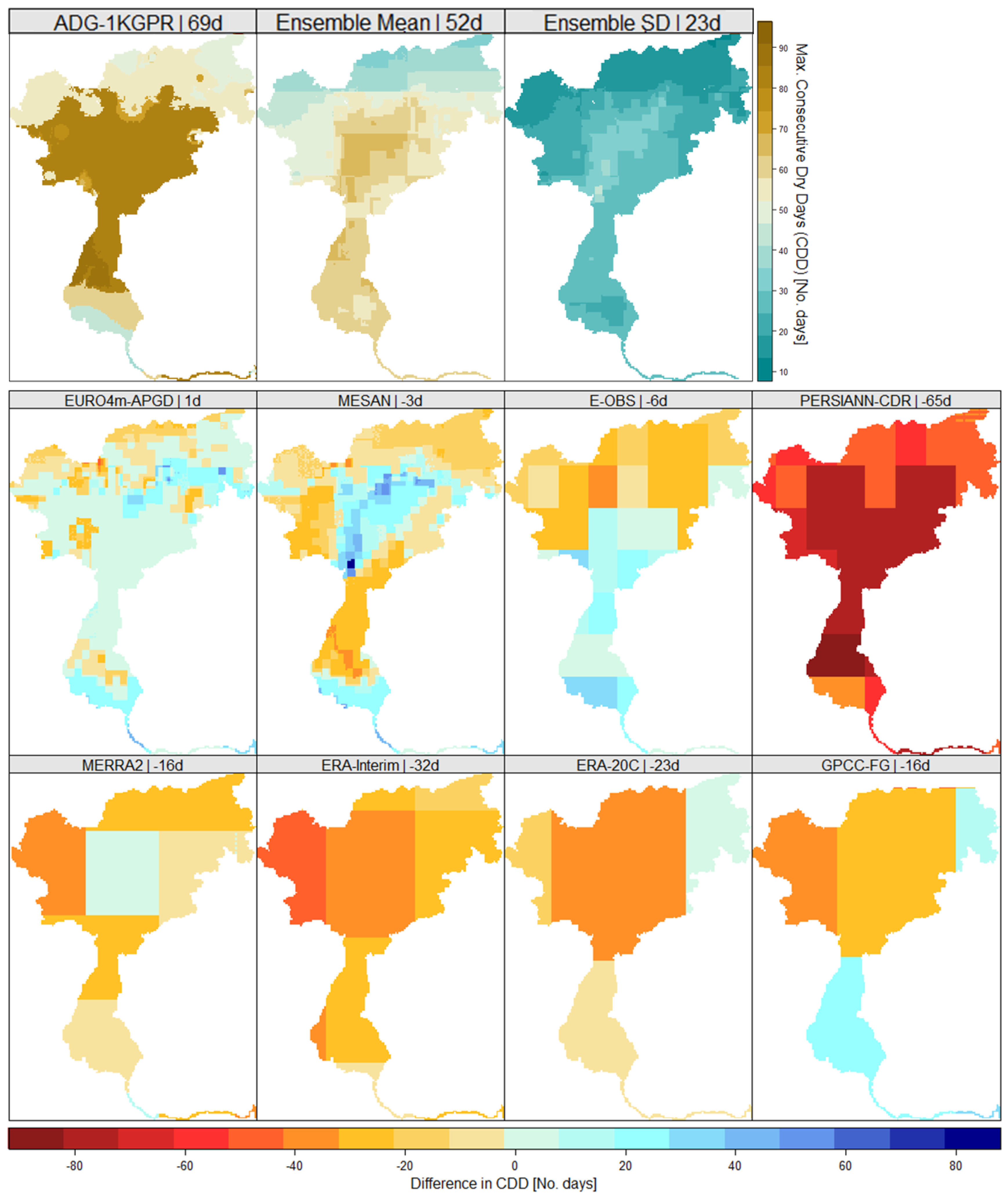
Figure 9.
Same as Figure 8 but for consecutive wet days (CWD).
Figure 9.
Same as Figure 8 but for consecutive wet days (CWD).

Figure 10.
Contribution of heavy precipitation (>95th percentile) to annual precipitation in % (R95pTOT) for the reference grid and the selected data sets.
Figure 10.
Contribution of heavy precipitation (>95th percentile) to annual precipitation in % (R95pTOT) for the reference grid and the selected data sets.

Figure 11.
Coefficient of Variation (CV) with respect to the source of the data sets for observational grids (blue) and reanalysis data sets (red), compared to CV introduced only by elevation (boxplots, black).
Figure 11.
Coefficient of Variation (CV) with respect to the source of the data sets for observational grids (blue) and reanalysis data sets (red), compared to CV introduced only by elevation (boxplots, black).

Figure 12.
Indicators for the selected grids ensemble, (a) mean annual precipitation in mm; (b) R95pTOT in %; (c) CDD in number of days; and (d) CWD in number of days.
Figure 12.
Indicators for the selected grids ensemble, (a) mean annual precipitation in mm; (b) R95pTOT in %; (c) CDD in number of days; and (d) CWD in number of days.


Table 1.
Overview of data sets included in this study with corresponding spatial resolution, temporal coverage, data set type or source respectively, and reference publication.
Table 1.
Overview of data sets included in this study with corresponding spatial resolution, temporal coverage, data set type or source respectively, and reference publication.
| Data Set | Resolution | Temporal Coverage | Type/Source | Reference |
|---|---|---|---|---|
| MESAN | 5 km | 1989–2010 | Downscaling/Reanalysis | [15] |
| EURO4m-APGD | 5 km | 1971–2008 | Observations | [14] |
| E-OBS v. 11 | 25 km | 1950–2015 | Observations | [20] |
| PERSIANN-CDR | 0.25° (~30 km) | 1983–present | Multisatellite (infrared), corrected | [19] |
| MERRA-2 | 0.5° latitude × 0.625° longitude (~50 km) | 1980–present | Reanalysis | [53] |
| ERA-Interim | 0.75° (~80 km) | 1979–present | Reanalysis | [11] |
| GPCC–FDD v1.0 | 1.0° (~100 km) | 1988–2013 | Observations | [12] |
| ERA-20C | 125 km | 1900–2010 | Reanalysis | [54] |
© 2017 by the authors. Licensee MDPI, Basel, Switzerland. This article is an open access article distributed under the terms and conditions of the Creative Commons Attribution (CC BY) license (http://creativecommons.org/licenses/by/4.0/).
Share and Cite
MDPI and ACS Style
Gampe, D.; Ludwig, R. Evaluation of Gridded Precipitation Data Products for Hydrological Applications in Complex Topography. Hydrology 2017, 4, 53. https://doi.org/10.3390/hydrology4040053
AMA Style
Gampe D, Ludwig R. Evaluation of Gridded Precipitation Data Products for Hydrological Applications in Complex Topography. Hydrology. 2017; 4(4):53. https://doi.org/10.3390/hydrology4040053
Chicago/Turabian StyleGampe, David, and Ralf Ludwig. 2017. "Evaluation of Gridded Precipitation Data Products for Hydrological Applications in Complex Topography" Hydrology 4, no. 4: 53. https://doi.org/10.3390/hydrology4040053
Note that from the first issue of 2016, this journal uses article numbers instead of page numbers. See further details here.