Thermal Regime of A Deep Temperate Lake and Its Response to Climate Change: Lake Kuttara, Japan

Abstract

A deep temperate lake, Lake Kuttara, Hokkaido, Japan (148 m deep at maximum) was completely ice-covered every winter in the 20th century. However, ice-free conditions of the lake over winter occurred three times in the 21st century, which is probably due to global warming. In order to understand how thermal regime of the lake responds to climate change, a change in lake mean water temperature from the heat storage change was calculated by integrating observed water temperature over water depths and by numerical calculation of heat budget components based on hydrometeorological data. As a result, a temporal variation of lake mean water temperature from the heat budget calculation was very reasonable to that from the observed water temperature (determination coefficient R² = 0.969). The lowest lake mean temperature for non-freeze was then evaluated at −1.87 °C, referring to the zero level at 6.80 °C. The 1978–2017 data at a meteorological station near Kuttara indicated that there are significant (less than 5% level) long-term trends for air temperature (+0.024 °C/year) and wind speed (−0.010 m/s/year). In order to evaluate the effects of climate change on freeze-up patterns, a sensitivity analysis was carried out for the calculated lake mean water temperature. It is noted that, after two decades, the lake could be ice-free once per every two years.

1. Introduction

At present, global warming tends to increase ice-free days in the arctic to subarctic regions [1,2], though a temporal slowdown in the global warming in 1998–2013 was reported [3,4]. Following the Köppen-Geiger climate classification, the Hokkaido Island, Japan, belongs to the southernmost subarctic area (Type Dfa to Dfb), where some water regions increase ice-free days [2]. Three deep caldera lakes, Shikotsu (360.1 m deep at maximum), Toya (180.0 m deep at maximum), and Kuttara (148.0 m at maximum), Hokkaido, are located in the Shikotsu-Toya National Park. Shikotsu and Toya are known as secularly ice-free lakes [5,6,7], while Kuttara is normally ice-covered in winter. Daily ice-covered conditions of Lake Kuttara have been observed by two curators, Ms. Naoko Mayeda and Mr. Hideyuki Sakamoto, of the Bear Museum at site B (Figure 1) since 1980s. According to their report, Lake Kuttara, located between Shikotsu and Toya, was completely ice-covered in the 20th century, when ice-ridge lines were often built up [8]. However, Kuttara was completely ice-free in 2004, 2007, and 2009, and partly ice-covered only one day in 2015, due to relatively warm winters. Even if ice-covered, the lake tends to shorten the ice-covered periods [9]. Non-freeze or shortening ice-covered periods could affect the aquatic ecosystem, because the solar radiation input then increases and nutrient input by snowmelt and rainfall runoffs from the surrounding catchment slope occurs at any time.

How lakes are ice-covered and then the lake ice is grown is physically developed by Ashton [10], Aihara et al. [8], Gebre et al. [11], and Leppäranta [12]. Aihara et al. [8] simulated the ice growth in Lake Kuttara by applying a three-layered model of snow, snow ice and pure ice. Applying a one-dimensional multi-year model, MyLake, of Saloranta and Andersen [13], Gebre et al. [11] simulated lake ice phenology and annual maximum lake ice thickness in the Nordic region. The Nordic lakes are completely ice-covered in November–May, while Lake Kuttara is ice-covered in late January–mid-April at longest and was completely ice-free in 2004, 2007, and 2009, and partly ice-covered in 2015. Kuttara is, thus, suitable for the investigation of a critical thermal condition for freeze or non-freeze over winter. In this study, heat budget of subarctic Lake Kuttara is estimated for about 4 years, and the calculated heat storage change is compared with observed one from moored temperature loggers. An increase in the frequency of ice-free conditions for the future is predicted from significant long-term trends for air temperature and wind speed.

2. Study Area and Field Observations

A deep temperate lake, Lake Kuttara (42°29′57″ N, 141°10′55″ E; lake level, ca. 258 m above sea level abbreviated as “asl”; 4.68 km² in area), was formed 40,000 years ago by the volcanic eruption of the Kuttara Volcano (Figure 1). Kuttara is topographically closed, since it has no outflowing river. However, the lake is hydrologically open because groundwater outflow is estimated at 0.44 m³/s [14]. This outflow corresponds to a decrease in lake level at 7.6 mm/day. Kuttara is dimictic, where vertical overturn occurs twice per year (in late December and early to late April, when the lake is thermally uniform at about 4 °C). Thus, Kuttara belongs to “temperate” lakes in the lake classification [15], though Hokkaido is in the subarctic zone.

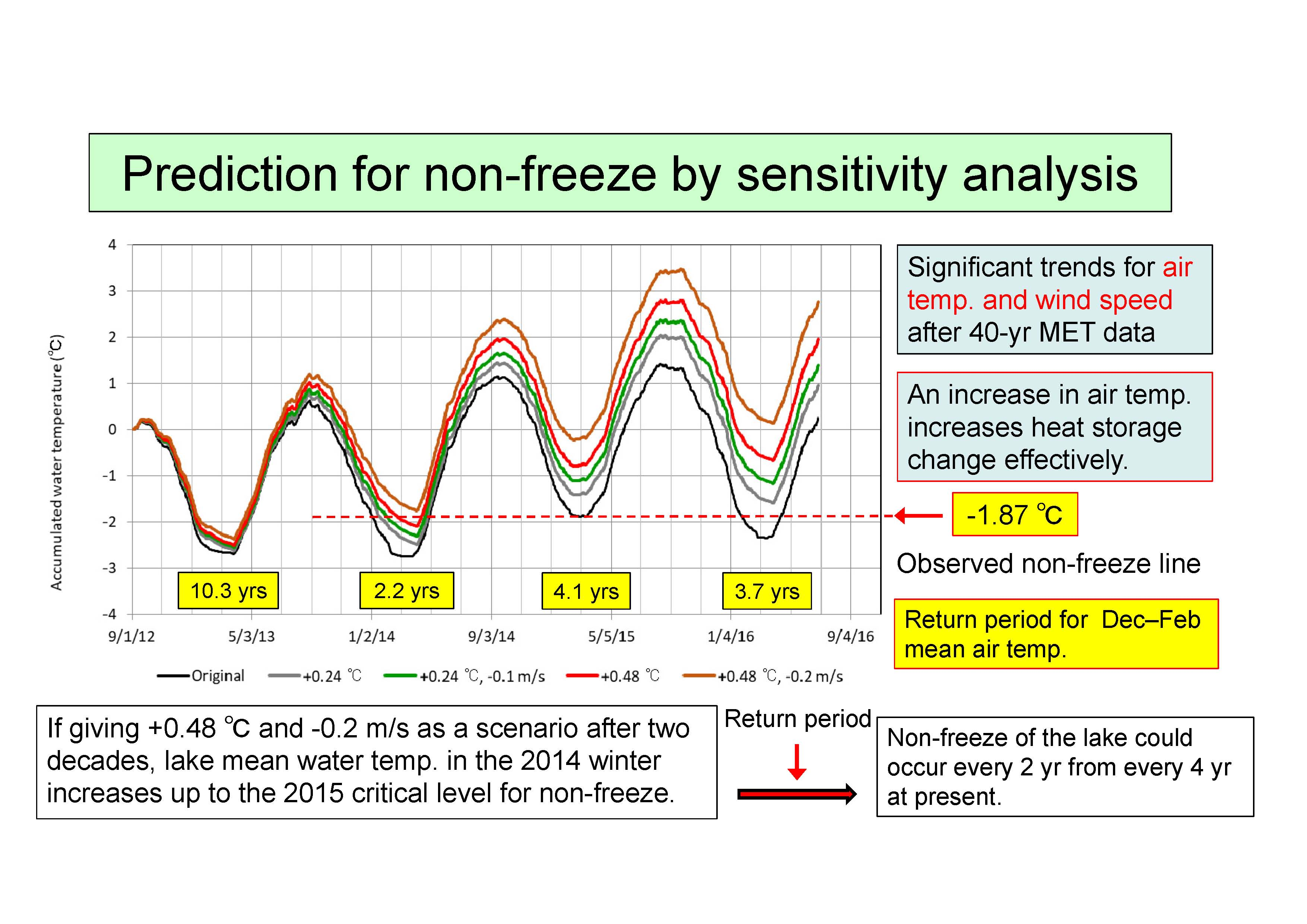
In order to estimate heat storage change of Lake Kuttara, 33 temperature data loggers were moored at the deepest point (site MD in Figure 1) on 1 September 2012 (Figure 2). The data loggers deployed are 20 Stowaway TidbiT, eight HOBO TidbiT v2 and five HOBO Pro v2 (accuracy, ±0.2 °C; Onset Computer Corporation, Bourne, MA, USA), which record water temperature at 30 min intervals. Since the accuracy of the temperature loggers is relatively low, they were calibrated by a standard thermometer (accuracy, ±0.02 °C) and a RINKO-profiler (model ASTD102, JFE Advantech, Co., Ltd., Nishinomiya, Japan; accuracy, ±0.01 °C) at a range of 0–35 °C.

The lake level seasonally varies with the amplitude of less than ca. 1.5 m. The mooring system in Figure 2 thus provides the depth-overlapping measurement of water temperature by the lowest four or five loggers below the surface marker buoy and the uppermost two loggers (140 m and 142 m above bottom) below the underwater buoy. In order to observe the heat flux at bottom, six loggers were fixed every 1 m depth above the bottom. Vertical profiles (0.1 m pitch) of water temperature from the profiler were obtained once per two months on average at seven sites, MD and P2–P7 during the loggers’ mooring (1 September 2012–30 June 2016). The profiler needs 15 to 26 min to get a vertical profile at each of the seven sites, and totally about 4 h to get vertical profiles at all the sites in the ice-free periods.

Meteorology (solar radiation, air temperature, relative humidity, rainfall, air pressure, and wind velocity) at the lake was observed at 30 min intervals at site M (ca. 3 m above the lake level), and water level at 30 min intervals at site L (Figure 1). Meteorology for data-missing periods was complemented from the linear relationship with data of AMeDAS (Automated Meteorological Data Acquisition System) Noboribetsu station (42°27′30″ N, 141°7′6″ E; 197 m asl) at 5.7 km southwest of site M and the Muroran Meteorological Observatory (42°18′42″ N, 140°58′30″ E; 39.9 m asl) at 25.8 km southwest of site M (correlation coefficient r = 0.852, 0.912, 0.805, 0.987, 0.995, and 0.734 for wind speed, air pressure, solar radiation, precipitation, air temperature, and relative humidity, respectively; p < 0.01). For snowfall and snow depth on the lake shore, the Noboribetsu data were utilized, assuming that the northern winter monsoon, producing snowfall, blows similarly at both Lake Kuttara and Noboribetsu. Rainfall or snowfall in winter was judged by air temperature and relative humidity at site M.

The lake level at site L was obtained at 30 min interval from a pressure data logger (model U20-001-01, HOBO Water Level Data Logger, Onset Computer Inc., USA; accuracy, ±0.3% FS for a range of 0–207 kPa) and air pressure at site M. Here, the calculated water depth (m) at site L was correlated with the lake level (m asl) from frequent topographic surveys, referring to the 1st class benchmark (no. H17-1-19; 42°29′35.2264″ N, 141°10′13.8119″ E; 263.682 m asl) of Geospatial Information Authority of Japan near site M. As a result, the observation error of lake level was about ±0.01 m. The lake level data are utilized at the daily mean base in the estimate of heat budget of the lake. Then, the effect of small and short surface oscillations such as surface seiche, wind wave, etc. can be neglected [16].

Inflow of some perennial streams is seen around site M. Their amount and water temperature were frequently measured in February to October. The non-freeze, partial freeze, or complete freeze of Lake Kuttara in winter has been judged by Mr. H. Sakamoto or Ms. M. Maeda, a curator of the Hokkaido Brown Bear Museum at site B since 1980s. As a result, the lake was completely ice-covered in the winters of 2013, 2014 and 2016, but partially ice-covered only one day in the winter of 2015. The thickness and inner structure of lake ice and upper snow after complete freeze were examined at site MD on 19 March 2013 and 21 February 2014.

3. Observational Results and Discussion

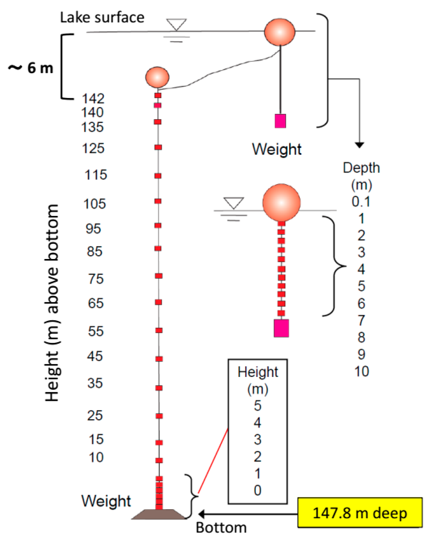
Figure 3 shows time series of daily mean air temperature and solar radiation, and daily mean water level (m asl) and daily precipitation for 2 September 2012–30 June 2016. The lake level varied with the amplitude of ca. 1.5 m, increasing in response to rainfalls, especially those in autumn. The increasing rate of lake level responding to rainfall is about 0.06 m per 50 mm/day. During relatively small rainfall at less than 10 mm/day or non-rainfall, the lake level decreases consistently. This is caused by the net groundwater output (groundwater outflow, ca. 0.4 m³/s, equivalent to ca. 7 mm/day) rather than evaporation (1–3 mm/day) at water surface [14]. When the day of 1st May is adopted as the first day of a hydrological year for the lake, the three years of 1 May 2013–30 April 2014, 1 May 2014–30 April 2015 and 1 May 2015–30 April 2016 showed total precipitation at 2182 mm (rainfall 93.6%, snowfall 6.4%), 2143.5 mm (rainfall 95.0%, snowfall 5.0%) and 1665 mm (rainfall 93.9%, snowfall 6.1%), respectively. As a result, the relatively small rainfalls in the final year induced very small fluctuations of lake level (Figure 3), when the rainfalls are likely balanced by the net groundwater output. Stream inflow near site M was totally less than 0.01 m³/s at water temperature of 3–23 °C.

Air temperature averaged over 1 December–28 or 29 February was −5.6 °C in December 2012–February 2013, −3.5 °C in December 2013–February 2014, −1.4 °C in December 2014–February 2015 and −2.7 °C in December 2015–February 2016. Meanwhile, the lake was completely ice-covered for 82 days (25 January–16 April) in 2013, 57 days (8 February–5 April) in 2014, and 31 days (23 February–24 March) in 2016, and partially ice-covered (70% area) only for one day (12 January 2015). Thus, ice-covered conditions of the lake are likely controlled by the winter temperatures, where −1.4 °C in 2015 seems to be critical for freeze or non-freeze (i.e., ice-free at more than −1.4 °C). In order to know the other critical condition for freeze or non-freeze, the sum, F, of negative degree-days before complete freeze was calculated [17]. As a result, F = 308.8 °C·day for 19 November 2012–25 January 2013 (completely frozen), 303.5 °C·day for 11 November 2013–8 February 2014 (completely frozen), 299.7 °C·day for 22 November 2015–23 February 2016 (completely frozen), and 264.4 °C·day for 14 November 2014–8 April 2015 (a final negative-degree day). Thus, the lake could be completely ice-covered at F > ~ 300 °C·day, and completely ice-free at F < ~260 °C·day. The duration with negative air temperature before complete freeze is shortest (50 days) in the winter of 2012–2013, but the mean air temperature was then lowest at −4.3 °C. Hence, it is seen that the efficiency of cooling down to complete freeze was highest in 2012–2013.

Observations at site B offered ice-covered processes in the lake by two ways; one is pure-ice extension from lake shore by natural cooling, and the other is snow-ice formation from relatively large snowfall onto water surface. In the latter way, the lake was completely ice-covered in about a day. F values during the complete freeze were 287.9 °C·day in 2012–2013, 166.0 °C·day in 2013–2014, and 81.5 °C·day in 2015–2016. If the lake ice grows as snow-free ice following the Stefan’s law, the ice thickness of 2012–2013 could be about twice as large as that of 2015–2016. In reality, the complete freeze of 2012–2013 and 2015–2016 occurred by snow-ice formation from 7 cm snowfall of 24 January 2013 and by pure-ice extension from natural cooling, respectively. The snow depth on ice after complete freeze temporally changed from 2 cm to 36 cm. Hence, the ice growth needs to be simulated by calculating the heat flux at interfaces of air-snow, snow-ice and ice-water.

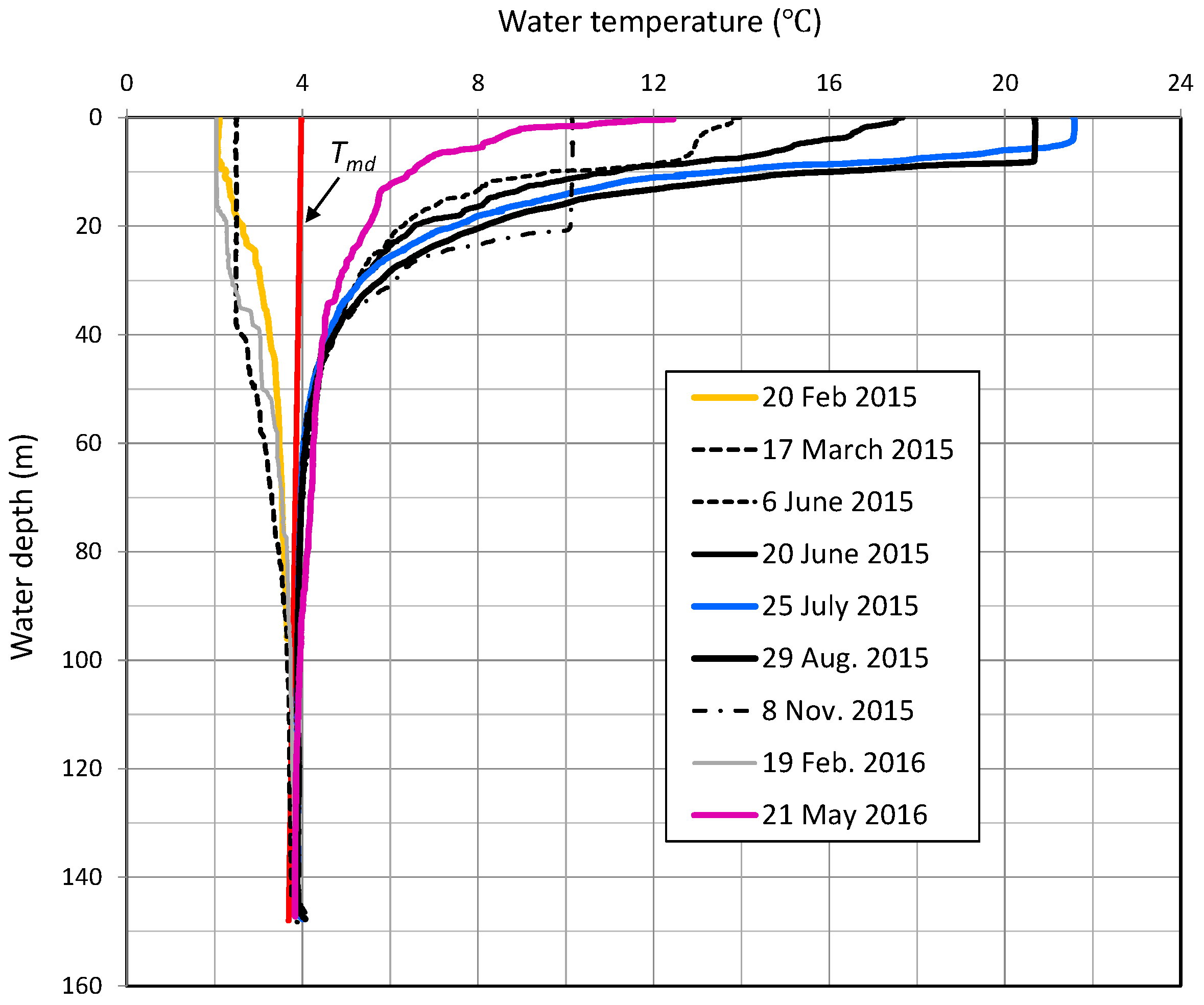
Figure 4 shows vertical distributions (0.1 m pitch) of water temperature at site MD in February 2015–May 2016. The T_md line depicts water temperature (°C) giving maximum density under water pressure and salinity at a certain water depth [6], and, in case of Lake Kuttara, 3.69 °C at 148.0 m. Lake Kuttara was partially ice-covered only on 12 January 2015, and completely ice-covered for 23 February–24 March 2016. Thus, the temperature profiles of 20 February 2015 and 19 February and 21 May 2016 in Figure 4 have no 0 °C layers at surface because of no ice. On 20 February 2015, the surface temperature was ca. 2 °C with the ca. 4 °C layer at depths of more than 100 m. Thus, the lake was thermally stratified even under completely ice-free condition. It is seen that, at depths of more than 90 m, the temporal change of water temperature is less than 1 °C. During the intense stratification of June–August, the bottom temperature at 3.86 °C (6 June 2015) increased up to 4.07 °C (29 August 2015). Since the heat flux toward the bottom is little in hypolimnion under the strong stratification, the increase in bottom temperature probably depicts the leakage of relatively warm water with some dissolved solids from below the bottom [18,19]. In fact, a geophysical survey by the magnetotelluric (MT) method in the Kuttara caldera suggests that there is a reservoir of geothermal water below the bottom at the deepest point [20]. When the lake is ice-free throughout the year, such an increase in bottom temperature is not seen in December–March. It is because the vertical circulation in the lake, which prevails during the weak stratification or approximately isothermal conditions in December–March, tends to dissipate the leaked water [18,21]. At the other points, such an increase in bottom temperature was not observed. Hence, the leakage from bottom seems to be confined to the deepest point or around (Figure 1).

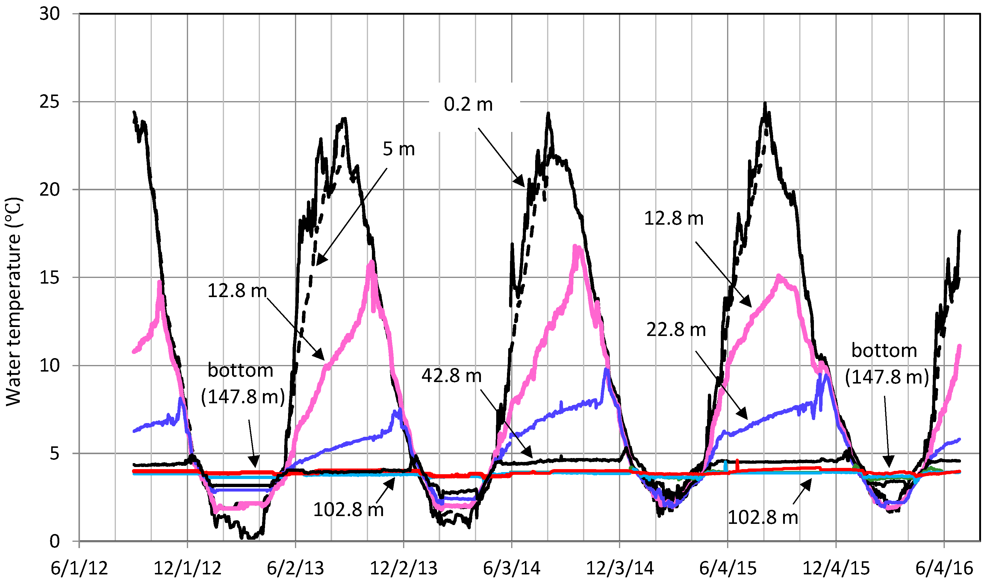
Figure 5 shows time series of daily mean water temperature from 0.2 m depth to the bottom (147.1–148.9 m in depth) for 2 September 2012–30 June 2016. The depths of more than 10 m are those averaged over the observed periods. The lake was completely ice-covered for 82 days in 2013, 57 days in 2014, and 31 days in 2016. It is seen that, as the ice-covered periods are longer, the water temperatures at 0.2 m, 5 m and 12. 8 m approach to 0 °C. This means that the upper layer is cooled by downward growth of pure ice [8]. In 2015 partially ice-covered, water temperature at depths of less than 42.8 m changes very similarly at less than 4 °C. This suggests that, during and after the pressure sensitive phase of the surface layer crossing the T_md line, wind mixing and an internal seiche initiated by wind produced gravitational instability and mixing by depressing a part of the negative temperature gradient to below the T_md line [21,22]. Thus, the investigation of the cooling process in a lake is needed to understand how the lake freezes and grows ice year by year [8,12,21]. The water temperature at 0–5 m above the bottom (Figure 2) varied over 3.6–4.1 °C. The heat flux from bottom may thus be evaluated, because the temperature difference is more than the accuracy of the loggers.

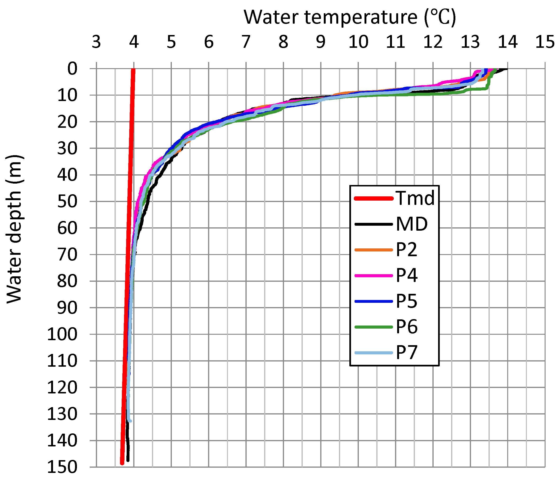
Figure 6 shows vertical distributions of water temperature at six sites, MD and P2, P4–P7 on 6 June 2015 (Figure 1). The temperature difference between the six profiles at a certain depth was ca. 1 °C at maximum. The small difference is due to both the small stream inflow (without prevalent river-induced currents) and active horizontal mixing by the sea wind in daily land-sea wind cycles or from episodic cyclones in the Pacific Ocean [16]. Here, the difference of ca. 1 °C is regarded as a maximum error in estimating heat storage changes of the lake from the daily mean temperature only at site MD (Figure 5). At depths of 70–140 m, the temperature at six sites is close to the T_md line. This suggests that the vertical circulation in spring occurred enough at these depths. At depths of 140 m, however, geothermal-water leakage after the circulation seems to slightly increase the temperature, thus being a little far from the T_md value [18].

4. Heat Storage Change of the Lake

Here, the heat storage change of Lake Kuttara will be numerically obtained by two ways; by direct measurements of water temperature and water level, and by the heat budget estimate. The ways are connected by the following equation:

$$\Delta G/\Delta t=\left(\Delta \left({{\displaystyle \int }}_{-h}^0\left({\rho }_w{c}_{p}T\left(z\right)A\left(z\right)dz\right)/\Delta t\right)\right)/A_0=R_n-Q_H-Q_E+Q_P+H_{Rin}+H_G+H_S$$

(1)

where ΔG is heat storage change (J/m²) of a lake for a budget period Δt (s), h is water depth (m) at deepest point, ρ_w and c_p are water density (kg/m³) and specific heat of water (J/kg/K) at temperature T (K), respectively, A is lake area (m²) at a depth, z (m) (A = A₀ at lake surface, z = 0), R_n is net radiation (W/m²), Q_H is sensible heat flux (W/m²), Q_E is latent heat flux (W/m²), Q_P is heat flux (W/m²) by direct precipitation onto the lake, H_Rin is heat flux (W/m²) by river inflow, H_G is heat flux (W/m²) by net groundwater inflow, and H_s is heat flux (W/m²) at lake bottom. Lake area A(z) is here acquired at 5 m depth interval by using the 1/10,000-scale bathymetric map published by Geospatial Information Authority of Japan. H_G and Q_P in Equation (1) are given as follows:

H_G = H_Gin − H_Gout = ρ_wC_p(G_in(T_Gin − T_l) − G_out(T_Gout − T_l))/A₀

(2)

$$Q_p={\rho }_w{C}_{p}P\left(T_p-T_s\right)$$

(3)

where G_in and G_out are groundwater inflow and outflow (m³/s), H_Gin and H_Gout are heat fluxes (W/m²) by groundwater inflow and outflow, respectively, T_Gin, T_Gout and T_l are temperatures (K) of inflowing and outflowing groundwaters and lake mean water temperature, respectively, P is precipitation (m/s) onto lake surface, T_P is temperature (K) of precipitation (here, assumed to be equal to the dew-point temperature), and T_s is water temperature at lake surface. Here, daily means of the meteorological factors, lake level and temperatures were utilized for a budget period, Δt = 86,400 s. In case of snowfall onto the lake, latent heat of ice from the negative air temperature to 0 °C and fusion heat of the 0 °C ice in water are reduced from Equation (3).

Net radiation R_n in Equation (1) consists of net shortwave radiation K* and net longwave radiation L*, as given by the following:

$$R_n=K^{*}+L^{*}=\left(1-\alpha \right)S_d+L_d-L_{up}=\left(1-\alpha \right)S_d+L_d-\epsilon \sigma T_{\mathrm{s}}^4$$

(4)

where S_d is downward shortwave radiation, α is albedo, L_d and L_up are downward and upward longwave radiations, respectively, ε is emissivity (here, 0.97 for ice (or snowy ice), water and snow, and 1.0 for air), and σ is Stefan-Boltzmann constant (=5.67 × 10⁻⁸ W/m²/K⁴). Referring to observational results of Brandt and Warren [23], α values of water, snow, ice (or snowy ice) and snowy water were given as constants of 0.05, 0.8, 0.5, and 0.3, respectively. The α values were then determined depending on lake surface conditions before and after complete ice cover, i.e., pure-ice extension from lake shore, snowy water (slush) just after snowfall, snowy ice after its freeze and snow accumulation on ice. Downward longwave radiation L_d was numerically obtained as a function of air temperature, total amount of effective water vapor content and relative sunshine duration [24].

Sensible heat flux Q_H and latent heat flux Q_E in Equation (1) were numerically obtained by the following bulk transfer method:

$$Q_H=(c{\rho }_a{a}_H{u}_z)\cdot \left(T_s-T_z\right)$$

(5)

$$Q_E=lE=-l\left(\frac{{\rho }_a\beta }{p}\right)\cdot \left(a_E{u}_z\right)\cdot \left(e_z-e_0\right)$$

(6)

where ρ_a is air density (=1.2 kg/m³), c is specific heat (J/Kg/K) of air under constant pressure, β is ratio of water vapor density to dry air density (=0.622), a_H and a_E are dimensionless bulk transfer coefficients for sensible heat and latent heat, respectively, u_z is wind speed (m/s) at z (m) above ground surface, T_z is air temperature (K) at z, T_s is surface temperature (K) at water surface, ice surface or snow surface, l is latent heat (J/kg) for evaporation, p is air pressure (Pa) at z, e_z is vapor pressure (Pa) at z, and e₀ is saturated vapor pressure (Pa) at T_s. Assuming the atmospheric condition to be neutral at any time, a_H = a_E ~ 1.5 × 10⁻³ was given for 1~ < u₃ < ~10 m/s [24]. During complete freeze, Q_E is zero at ice-water interface, and, instead, sublimation from ice or snow surface at less than 0 °C or evaporation at water surface of 0 °C (after rainfall) above ice surface was calculated. At T₃ > 0 °C, T_s = 0 °C is given, and the net heat flux, R_n − Q_H − Q_E + Q_P, at surface is then consumed as fusion heat of ice or snow. When the right side of Equation (1) was negative at ice-water interface after complete freeze, and also its absolute value is larger than the upward heat flux at ice-water interface, the consequent heat loss was replaced by pure-ice growth. Snow depth on ice after complete freeze was supposed to be equal to snow depth after the date of freeze at the Noboribetsu station. The integration of heat storage change between z = −h and 0 m in Equation (1) was numerically obtained by water temperature of 0–90 m depth, because of little temperature fluctuation at depths of more than 90 m (Figure 4).

5. Calculated Results

Figure 7 shows 5-day moving average for each of the thermal terms, K*, L_up, L_d, Q_P, Q_H and Q_E at water surface, ice surface or snow surface. Depending on the albedo of water surface, ice surface and snow surface, net shortwave radiation K* changes greatly, especially for a time period of complete freeze to the open water in early April or mid-April. The heat flux Q_p is given at −1.73 W/m² on average, at 16 W/m² at maximum, and at −19 W/m² at minimum for the observation period. The Q_P is relatively effective to cool the lake, when a large rainfall of more than 100 mm/day occurs in the cooling season of September-October. For example, the rainfalls of 106 mm/day and 265 mm/day on 11 and 25 October 2013 gave Q_P = −15.1 W/m² and −45.8 W/m², respectively. The heat flux H_Rin by river inflow is less than 1 W/m² at any time and thus is neglected. The heat flux H_s at bottom was evaluated at the order 1 W/m² at the deepest point [18,19]. The magnitude of H_s could be restricted to the deepest point or around, since the increase in bottom temperature was not observed at the other points (Figure 1). Thus, H_s is also neglected. For the ice-covered period, Q_H is consistently negative, thus heating ice or snow surface. Then, the net heat flux H_G by groundwater input and output in Equation (2) is estimated at 0.52 W/m² from G_in = 0.16 m³/s, G_out = 0.44 m³/s, T_Gin = 7.3 °C (annual mean air temperature), T_Gout = 4.0 °C and T_l = 4.2 °C [14,25]. The value of 0.52 W/m² probably corresponds to the annual minimum, since G_in tends to increase by rainfall. However, when G_in = 0.3 m³/s and T_l = 8 °C are supposed as those in the rainfall season, H_G is calculated at 1.4 W/m². Hence, in addition to H_Rin and H_s, the heat flux H_G is judged to be negligibly small compared with the heat budget components in Figure 7.

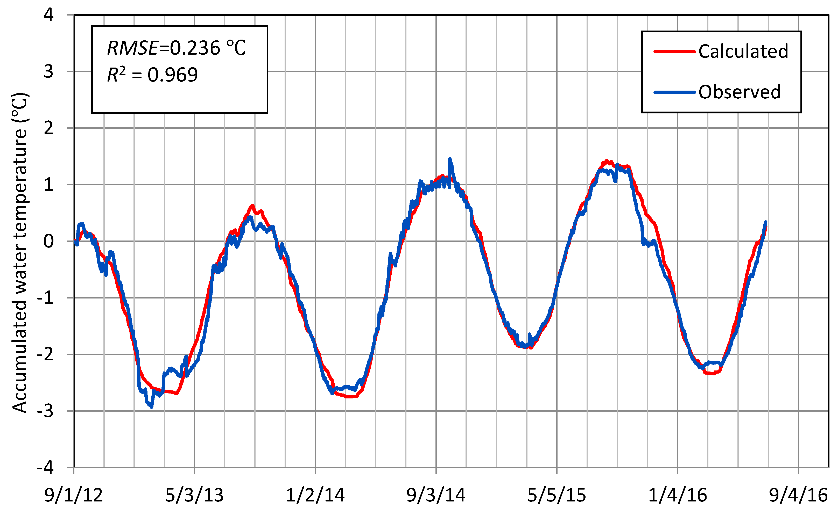
Figure 8 shows temporal variations of observed and calculated lake mean water temperature (°C) from the heat storage change ΔG/Δt (J/m²/day). Taking the lake mean water temperature, 6.80 °C, of 2 September 2012 as a reference level, a daily increment or a daily decrement of lake mean water temperature was calculated by dividing ΔG by (ρ_w·C_p·h_m), where h_m is the mean water depth (=106.6 m), and then was accumulated for 3 September 2012–30 June 2016. As a result, the lake mean water temperature from the heat budget calculation on the right side of Equation (1) is very reasonable to that from the observed water temperature with the determination coefficient R² = 0.969 and the root-mean square error, RMSE = 0.236 °C. Thus, the heat storage change can be reasonably acquired by data of meteorology, lake level, and surface water temperature. The observed water temperature in Figure 8 indicates that the lake is heated in mid-February–mid-August and cooled in mid-August–mid-February. In the winter of 2015, the lake was partly ice-covered only one day (12 January). Thus, this winter could provide a critical lake mean water temperature for ice-free conditions. As a result, the observed lowest water temperature is given at 4.93 °C (at –1.87 °C in Figure 8) as a threshold for non-freeze. The lowest water temperature in 2013, 2014 and 2016 was 4.06 °C, 4.19 °C and 4.55 °C, which correspond to the durations of complete freeze, 82 days, 57 days and 31 days, respectively.

6. Prediction for Non-Freeze

By sensitivity analysis for heat storage change from the heat budget calculation, Chikita et al. [26] revealed that the heat storage change of Lake Kuttara increases effectively with increasing air temperature. Applying the 1978–2017 data of the Noboribetsu meteorological station, it is seen that there are statistically significant long-term trends (less than 5% level) for annual mean air temperature and wind speed. As a result, an increasing rate of air temperature was given at +0.024 °C/year, and a decreasing rate of wind speed, at −0.01 m/s/year. Meanwhile, annual rainfall and precipitation did not depict any significant trends. Assuming the trends to be identical to those at the lake, it is possible to predict the occurrence of ice-free conditions for the future.

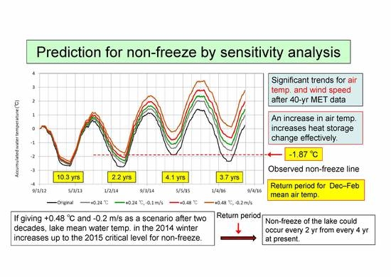
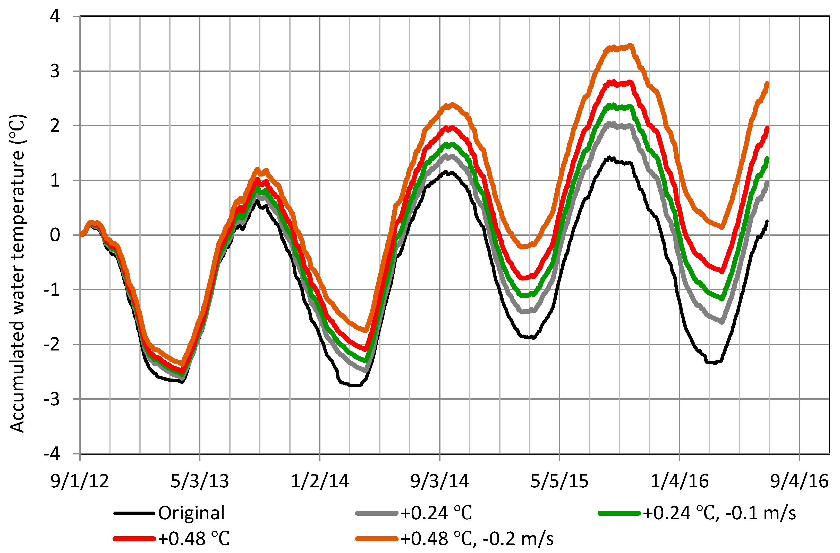
Figure 9 shows temporal variations of lake mean water temperature calculated under condition of air temperature at +0.24 °C and +0.48 °C and, in addition, wind speed at −0.1 m/s and −0.2 m/s. Applying the rates of +0.024 °C/year and −0.01 m/s/year for air temperature and wind speed, respectively, the increments of +0.24 °C and +0.48 °C and the decrements of −0.1 m/s and −0.2 m/s correspond to annual mean air temperature increased and wind speed decreased after a decade and two decades, respectively. As a result, the combination of +0.48 °C and −0.2 m/s increases the lowest water temperature in 2014 up to the critical water temperature in 2015. The increment of +0.24 °C and its combination with the decrement of −0.1 m/s are not enough to increase the lowest temperature in 2014 up to the critical one, but, instead, increases the lowest temperature in 2016 to the level above the criterion. Thus, the bidecadal and decadal increments and decrements could raise the lowest water temperatures in 2014 and 2016 to the non-freeze level, respectively. In the 40-year Noboribetsu data, return periods of mean air temperature in December–February are 2.2 years, 4.1 years, and 3.7 years for December 2013–February 2014, December 2014–February 2015, and December 2015–February 2016, respectively. Thus, in two decades, the ice-free condition could occur every ca. 2 years on average from every ca. 4 years at present. A return period of mean air temperature in December 2012–February 2013 was 10.3 years. If the lowest water temperature, 4.06 °C, in 2013 approaches to the critical level, 4.93 °C, for the future, Lake Kuttara may be secularly ice-free.

7. Conclusions

Data of meteorology, lake level and water temperature for a deep temperate lake, Lake Kuttara, were obtained for the period of 2 September 2012–30 June 2016, and heat storage change of the lake was numerically evaluated by two ways, i.e., by integrating observed water temperature over water depths and by the heat budget calculation based on hydrometeorologial data. The heat storage change obtained was expressed as a change in water temperature averaged over the lake, which was accumulated for 3 September 2013–30 June 2016. The lake mean water temperature, 6.80 °C, of 2 September 2012, was then chosen as a reference level. As a result, a change in lake mean water temperature from the heat budget calculation was very consistent at R² = 0.969 and RMSE = 0.236 °C with that from observed water temperature. In the winter of 2015, the lake is partly ice-covered only one day, while, in the winters of 2013, 2014, and 2016, it was completely ice-covered. Hence, the lowest lake mean water temperature, 4.93 °C, in 2015 was judged to be a threshold for non-freeze. Based on a sensitivity analysis for the change of lake mean water temperature, ice-free conditions of the lake for the future were discussed. Significant long-term trends from the 40-year meteorological data indicated +0.024 °C/year for air temperature and −0.01 m/s/year for wind speed. Hence, air temperature’s increments of +0.24 °C and +0.48 °C and the combination with wind speed’s decrements of −0.1 m/s and −0.2 m/s, were given as scenarios of thermal conditions after a decade and two decades, respectively. As a result, the scenario of +0.48 °C and −0.2 m/s increased the lowest lake mean water temperature in 2014 up to the non-freeze level. Considering the return periods of mean air temperature in December–February, after two decades, the non-freeze of the lake could occur every ca. 2 years from every ca. 4 years, at present.