Changes in Temperature and Rainfall as a Result of Local Climate Change in Pasadena, California


Water & Power Department, City of Pasadena, 150 S. Robles Ave., Suite 200, Pasadena, CA 91101, USA
Hydrology 2018, 5(2), 25; https://doi.org/10.3390/hydrology5020025
Submission received: 21 March 2018
/
Revised: 12 April 2018
/
Accepted: 18 April 2018
/
Published: 10 May 2018
(This article belongs to the Special Issue Climatic Change Impact on Hydrology)
Abstract
:The City of Pasadena is located in southern California, a region which has a Mediterranean climate and where the vast majority of rainfall occurs between October and April, with the period between January and March being the most intense. A significant amount of the local water supply comes from regional rainfall, therefore any changes in precipitation patterns in the area has considerable significance. Hypothesis: Local climate change has been occurring in the Pasadena area over the last 100 years resulting in changes in air temperature and rainfall. Air Temperatures: Between 1886 and 2016, the air temperature in Pasadena, California has increased significantly, from a minimum of 23.8 °C in the daytime and 8.1 °C at night between 1911 and 1920 to 27.2 °C and 13.3 °C between 2011 and 2016. The increase in nighttime temperature was uniform throughout the year, however daytime temperatures showed more seasonal variation. There was little change in the daytime temperatures for May through July, but more change the rest of the year. For example, the median daytime temperature for June between 1911 and 1920 was 27.9 °C but was 28.7 °C between 2011 and 2016, a difference of 0.8 °C. In contrast, for October for the same periods, the median daytime temperatures were 25.6 °C and 28.9 °C, a difference of 3.3 °C. Rainfall: There has been a change in local rainfall pattern over the same period. In comparing rainfall between 1883 and 1949 and between 1950 and 2016, there appeared to be less rainfall in the months of October, December, and April while other months seemed to show no change in rainfall. For example, between the two periods mentioned above, the median rainfall in October was 12.4 mm and 8.9 mm, respectively, while for December they were 68.6 mm and 40.4 mm. There was comparatively a smaller change in the median volume of rainfall in April (18.8 mm vs. 17.5 mm). However, between 1883 and 2016, there were 13 with less than 1 mm of rain, 12 of which occurred after 1961. In the same line of logic, no measureable amount of rain occurred for 23 Octobers, 15 of those occurring after 1961. Conclusions: As air temperatures increased over the last 100 years in the Pasadena area, rainfall may have decreased in October, December, and April.
1. Introduction
In a recently published study, it has been shown that median air temperatures have increased significantly in the City of Pasadena over the last 100 years [1], which resulted in significant stream flow changes in the Arroyo Seco. The paper argued that these changes in air temperature and stream flow were the result of Anthropogenic Climate Change (ACC). It would not be too surprising to speculate that rainfall in the Pasadena area would also be affected by ACC. Some models project changes in rainfall as a result of ACC in the southern California region [2]. This paper examines increasing air temperatures in the Pasadena region, compares them to broader regional changes, and then correlates them with changes in rainfall patterns. Actual local temperature and rainfall data is used and not downscaled global data [3,4,5].
2. Pasadena and Its Environment
The City of Pasadena is located in Los Angeles County, at the southern, windward side of the San Gabriel Mountains, which are approximately 1700 m high and 40 km from the Pacific Ocean. Pasadena is located 15 km north-east of downtown Los Angeles and sits atop of the Raymond Basin, an alluvial aquifer in the northwestern corner of the highly urbanized San Gabriel Valley. The area has a Mediterranean climate [6] with the overwhelming majority of rainfall occurring between October and April. Most of Pasadena is approximately 260 m (780 ft) above mean sea level but it ranges from 180 m (540 ft) to 460 m (1380 ft).
3. Study Design
3.1. Hypothesis
Southern California has been experiencing ACC and as a result, rainfall patterns have been and continue to be altered in the Pasadena area. The change in climate is shifting air temperatures unevenly which results in daytime and nighttime temperatures deviating at different rates and during different seasons. As a result, any changes in rainfall would not be uniform.
3.2. Study Design
- Organization: There are three parts to this study. The first two parts involves air temperatures in the City of Pasadena for evidence of local climate change. The third part examined changes in rainfall in Pasadena.
- Periods:
- The Study Period covered the 1880s to 2016 depending on the location.
- The Base Period covered the years 1910–2000 and was used a baseline for changes in temperature.
- The Control Period covered all years prior to 1950.
- The Test Period covered 1950 and all subsequent years.
- These Control and Test Periods were selected to divide the rainfall data into two equal halves and the air temperatures into two approximately equal populations.
- Part 1: The average annual surface temperatures differences from the long term mean temperature were determined for each year between the Study Period. Then, the annual average temperature for each was compared to the average temperature of the Base Period. The difference between the annual average temperature of each year and the Base Period was calculated. This was done for the surface temperatures for the entire globe, the Northern Hemisphere, North America, California, and Pasadena. If the average annual temperature difference increased in parallel to changes seen in the broader data sets, there would be evidence for local climate change.
- Part 2: The daytime and nighttime temperatures for Pasadena were analyzed separately. If the daytime or nighttime temperatures increase or decrease significantly between 1885 and 2016, that would be an indication that climate change has been occurring. The record for 1885 was incomplete so it was not used in Part 1, but it would be useful for Part 2 for some months.
- Part 3: The second component involves measuring rainfall in the Pasadena area between 1883 and 2016 to determine if there has been a significant change in rainfall.
3.3. Statistical Procedures
- Normality. The normality of each data set was assessed using the Kolmogorov–Smirnov test. Air temperatures and rainfall in all study periods were non-normally distributed (p < 0.001); the results were strongly skewed and kurtotic. This means that rather than being distributed in a normal bell-shaped curve with data evenly balanced on both sides of the mean, more data was on one side than the other and the shape of the curve was wider than expected. Almost all of the data in this paper was non-normally distributed.
- Comparisons of Two Groups. When the rainfall and air temperature data were compared pairwise, the Mann–Whitney Rank Sum Test (MWRST) was used. This is the nonparametric equivalent to the Student’s t-test. The U values are calculated and the probability (p) that these represent significant differences was determined.
- Comparisons of More than Two Groups. The air temperature data was grouped based on decade and were compared to the most recent decade, the Kruskal–Wallis One-Way Analysis of Variance on Ranks (KW) was used. If a significant difference was determined to be present, i.e., if the Kruskal–Wallis Statistic (H) is above the critical value, then each group was compared against a control group using Dunn’s Test. Dunn’s Test produces a Studentized Range value, q, which is assessed in the same fashion as the Student’s t-test critical values with probabilities and critical values corresponding to levels of probability, α, of incorrectly rejecting the null hypothesis.
- Correlations. When temperature data from different locations was compared to determine if they tend to track each other, the Spearman Rank Order Correlation (SPOC) was used. The SPOC is the nonparametric equivalent to the Pearson Product Moment Correlation. The greater the correlation coefficient (R), the more the two sets of data track each other.
- Extreme Values. The rainfall data was also assessed for extremes. The number of driest and wettest months were calculated for each period using the Fisher Exact (FE) Test.
The critical value for this study for α was 0.05 for KW, MWRST, SROC, and FE tests [7].
3.4. Data Acquisition and Assessment
- Air-PWP has extensive written records of atmospheric temperatures in Pasadena dating back to the 1880s, collected mostly by the employees of the City of Pasadena, but the records from 1882 to 1890 were collected by a private resident of Pasadena, Dr. Thomas Rigg. However, there are two significant gaps in the temperature records, one between 1890 and 1893 and the other between 1895 and 1908. The first gap is the time between when Dr. Rigg stopped collecting data and when the City started collecting data. The second gap was caused in part by the loss of paper records stored by the Department of Commerce in San Francisco following the earthquake and fire of 1906. The records were supplemented by and checked against records from the National Oceanic and Atmospheric Administration’s National Climatic Data Center (NOAA-NCDC). A database of the daily maximum temperature (all maximum temperatures occurred during the daylight hours are referred as “daytime temperatures”), minimum temperatures (all minimum temperatures occurred during the nighttime hours are referred as “nighttime temperatures”), and precipitation were created and checked for accuracy (paper records vs. electronic, missing data, and obvious outliers). A database of air temperatures was created with both the daytime (n = 41,201) and nighttime temperatures (n = 45,964) for Pasadena (most of the data was collected at City Hall, +34.15, −118.14 while other data were all collected within a kilometer of it). The temperature differences between the base period and each individual year was downloaded from the National Centers for Environmental information, Climate at a Glance: Global Time Series [8].
- Rainfall—The City of Pasadena began officially collecting rainfall data with its own staff in 1883 near the same location used for measuring temperature. Later, this site was coordinated with NOAA. Rainfall data was downloaded from the same webpage as the temperature data and the two databases were crosschecked.
4. Results
4.1. Part 1
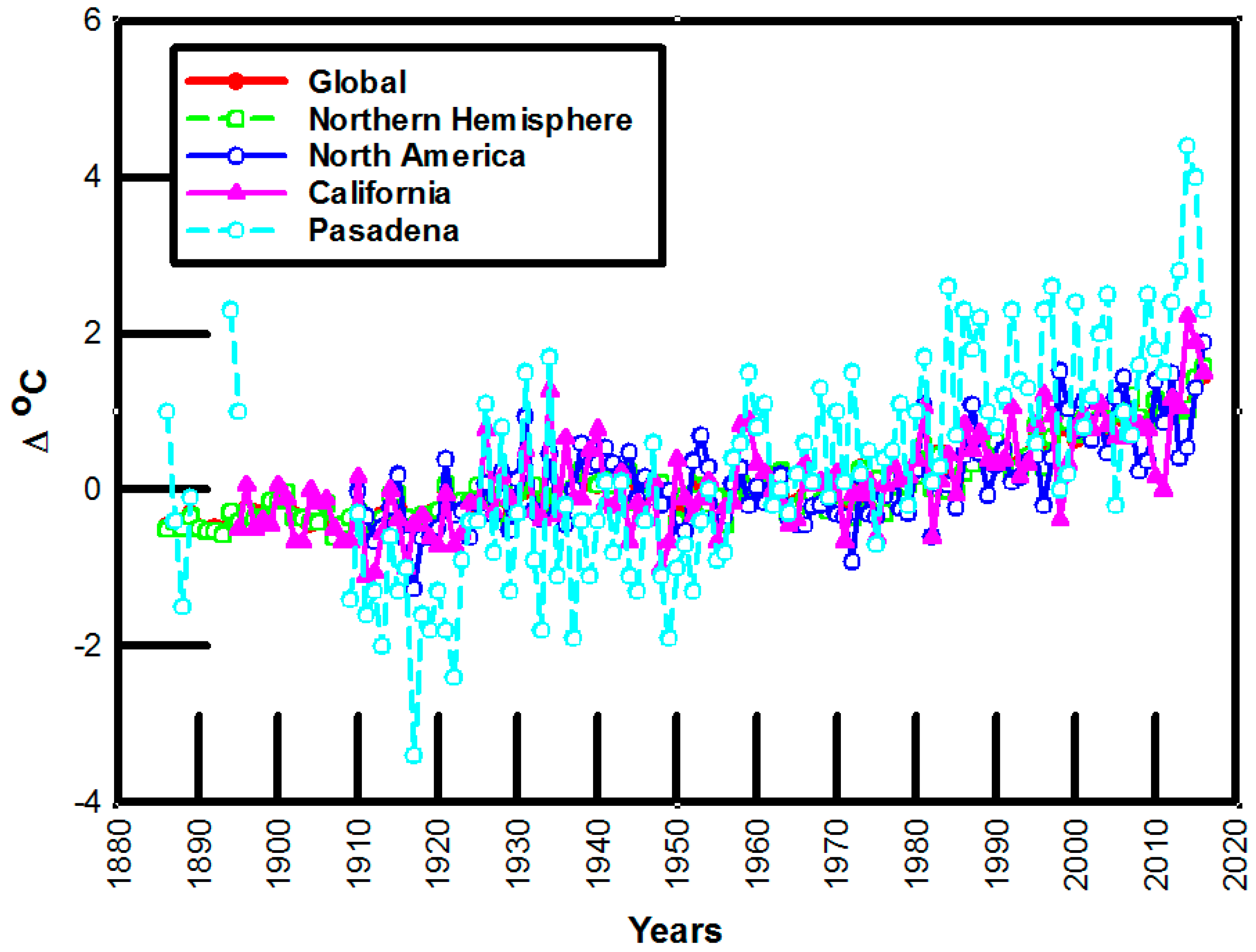
Table 1 summarizes the annual average diviations from the Base Period for surface temperatures for the entire earth (Global), the Northern Hemisphere (NH), North America (NA), California (Cal), and Pasadena. In all cases, the mean and median differences in surface temperature were lower than the Base Period before 1950 and higher after 1950 to a statistically significant degree. The mean and median differences very similar, about −0.2 °C for the Control Period and about +0.2 °C for the Test Period. The data from California were slightly more extreme for both periods. The data from Pasadena was much more extreme, −0.9 °C for the Control Period and +0.8 °C for the Test Period. If the Control Period data for the five areas are compared by using the KW test, there is a significant difference (H = 25, p < 0.001). Using Dunn’s Test, the Pasadena data was significantly lower than the Global data (Q = 3.83, p = 0.001), lower than the Northern Hemisphere data (Q = 3.99, p < 0.001), and lower than the North American data (Q = 4.45, p < 0.001). Although lower than the California data, the Pasadena data was not significantly lower (Q = 2.76, p = 0.06) although only just barely. Conversely, if the Test Period data for the five areas are compared by using the KW test, there is a significant difference (H = 21, p < 0.001). Using Dunn’s Test, the Pasadena data was significantly higher than the Global data (Q = 4.61, p = 0.010), lower than the Northern Hemisphere data (Q = 4.73, p = 0.007), lower than the North American data (Q = 5.88, p < 0.001), and lower than the California data (Q = 4.36, p = 0.018). The SROC showed that the changes in the data among all locations tended to track one another, although the Pasadena data showed the least correlation with other locations. The data from all five locations was plotted over time in Figure 1.
4.2. Part 2
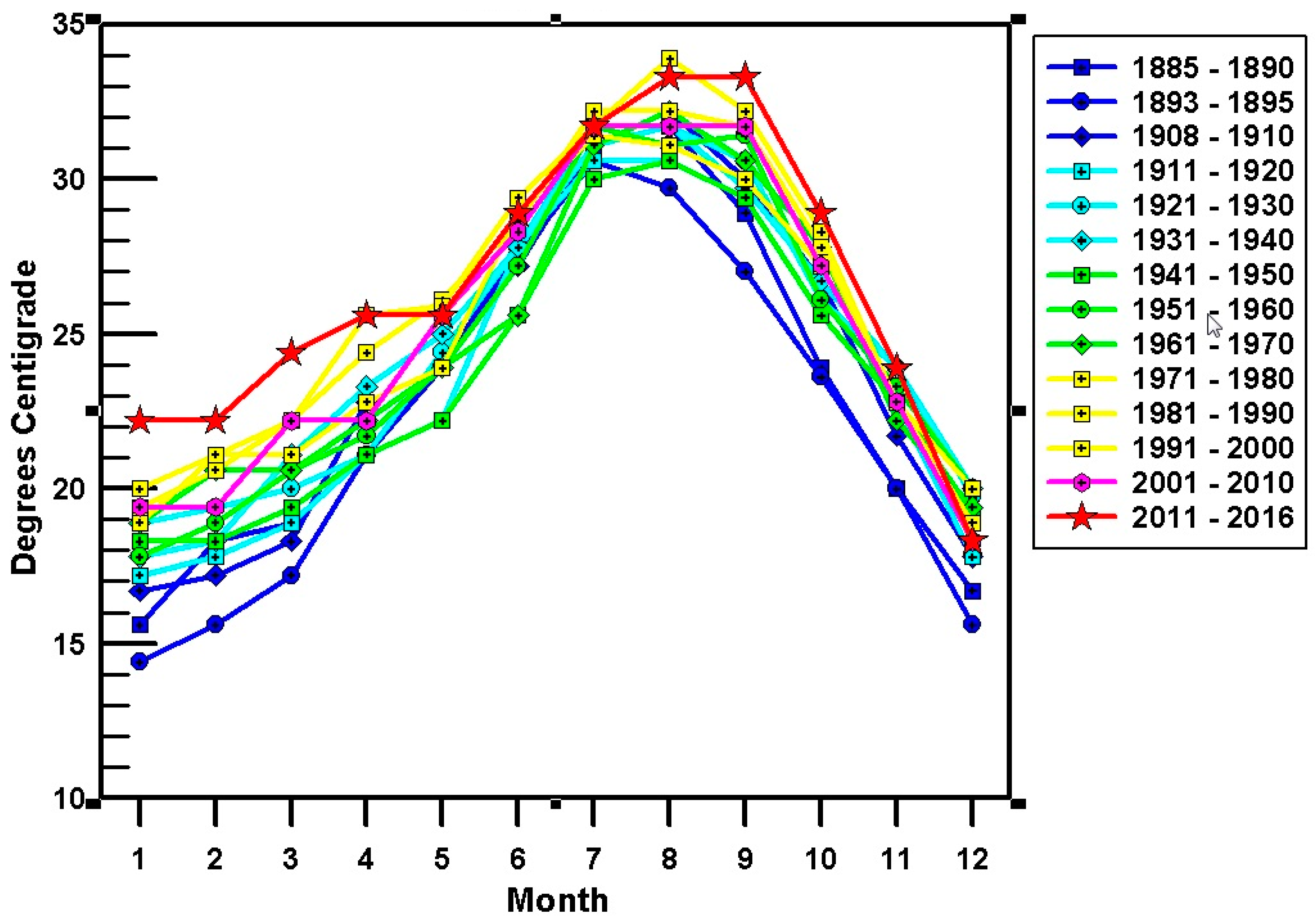
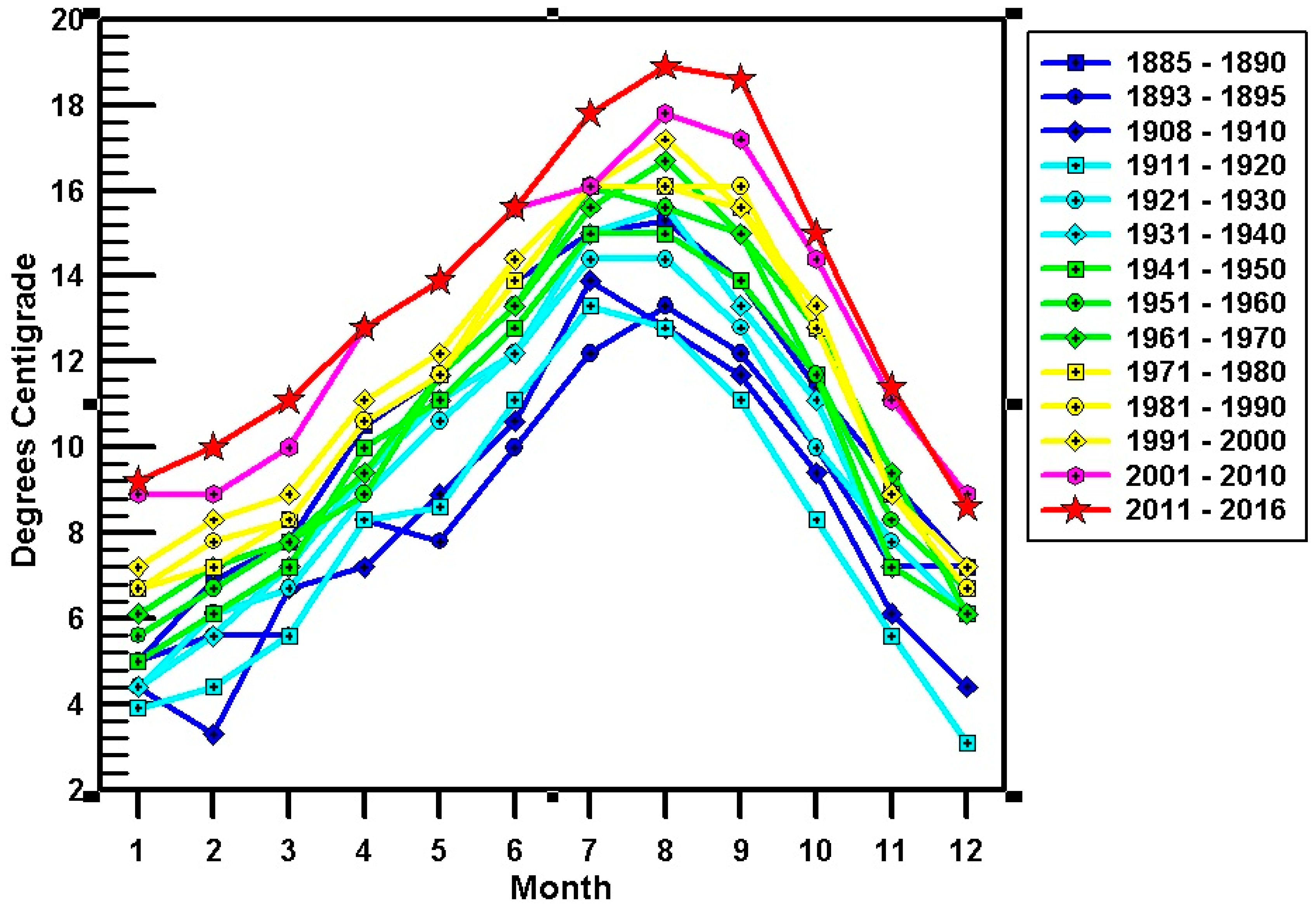
All of the daily maximum (daytime) and minimum (nighttime) temperatures recorded in Pasadena between March of 1885 and December 31, 2016, the Study Period, are summarized in the first line of Table 2 and Table 3, respectively. The two groups were tested using MW. Table 2 shows the number of daily maximum readings for the entire Study Period, the Control Period, and the Test Period for all years and each month as well as the mean, median, 25th percentile, 75th percentile, and the results of the MWRST. Table 3 shows the same results for daily minimum readings for the entire year and for each month separately. Both the daytime and nighttime results were non-normally distributed. In all cases but one, (November daytime temperatures), the Test Period had significantly higher temperatures than the Control Period. The data was then divided up by decades, 1881–1890, 1891–1990, etc., and plotted against the month and are shown in Figure 2 and Figure 3 for daytime and nighttime temperatures, respectively. The November daytime temperature divided by decade was tested using the KW test and it was shown that there was a significant difference (H = 97 with 13 degrees of freedom p ≤ 0.001). Using Dunn’s Test and using the 2011–2016 period as a control, the q value for the decade of 1881–1890 was 6.8 (p < 0.001), for 1891–1900 it was 4.1 (p < 0.005), for 1901–1910 it was 3.5 (p < 0.01), and all other decades had a q value of 2.5 or less which was not significant (p > 0.05). The mean daytime temperatures for the decade of 1881–1890 was 20.0 °C (n = 150), for 1891–1900 it was 20.0 °C (n = 60), for 1901–1910 it was 21.7 °C (n = 90), and for 2011–2016 it was 23.9 °C (n = 171).
Overall, the daytime median temperatures increased by 5% between the Control Period and the Test Period (24.4 °C to 25.6 °C, a difference of 1.2 °C) however, the amount of that increase varied considerably for different months. Generally, colder months showed larger increases than warmer months. Figure 2 shows that the median temperatures in the winter months, such as January, were considerably greater than in summer months, such as July. In Table 2, the median air temperature increased 9% in January between the Control Period and the Test Period but in July, the median air temperature only increased 2%, while in November there was no measurable increase at all.
The nighttime air temperatures showed a much larger and more consistent increase. The median nighttime temperatures increased by 24% (9.4 °C to 11.7 °C or 2.3 °C), which is larger both in absolute terms and as a percentage. In Table 3 and Figure 3, every month showed large increases in the median nighttime temperature as compared to daytime temperatures. However, there were still considerable variations between months. Colder months showed greater increases than warmer months. January showed the largest difference between the Control Period and the Test Period, 2.8 °C or a 64% increase, while July only showed a 2.3 °C change or a 16% increase in median air temperature.
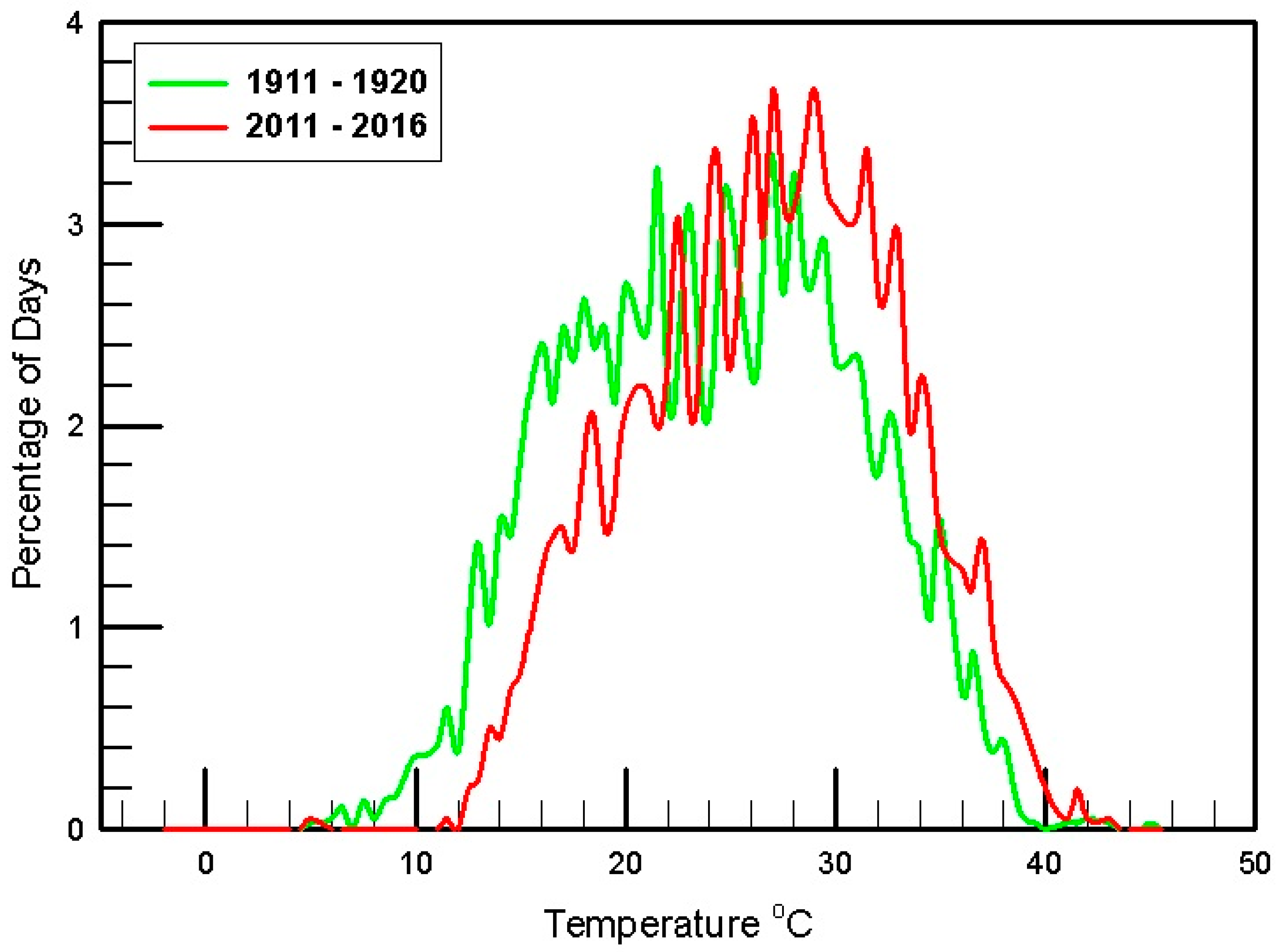
To further assess the nature of these temperature changes, the same data used in Figure 2 and Figure 3 were recalculated as a frequency. The percentage of days within a given range of temperatures was calculated and plotted in Figure 4. For clarity, only two decades are shown, the period between 1911 and 1920 and the period between 2011 and 2016. There is little change in the frequency distribution of hotter days while there has been much more of a change during colder days. For example, in the 1911–1920 period, there are a substantial number of days with a maximum temperature of less than 10 °C, while in the 2011–2016 period there are almost none. In contrast, the number of days with a maximum daytime temperature above 40 °C has hardly changed at all. This would create the impression that there is a maximum daytime temperature that is generally not exceeded.
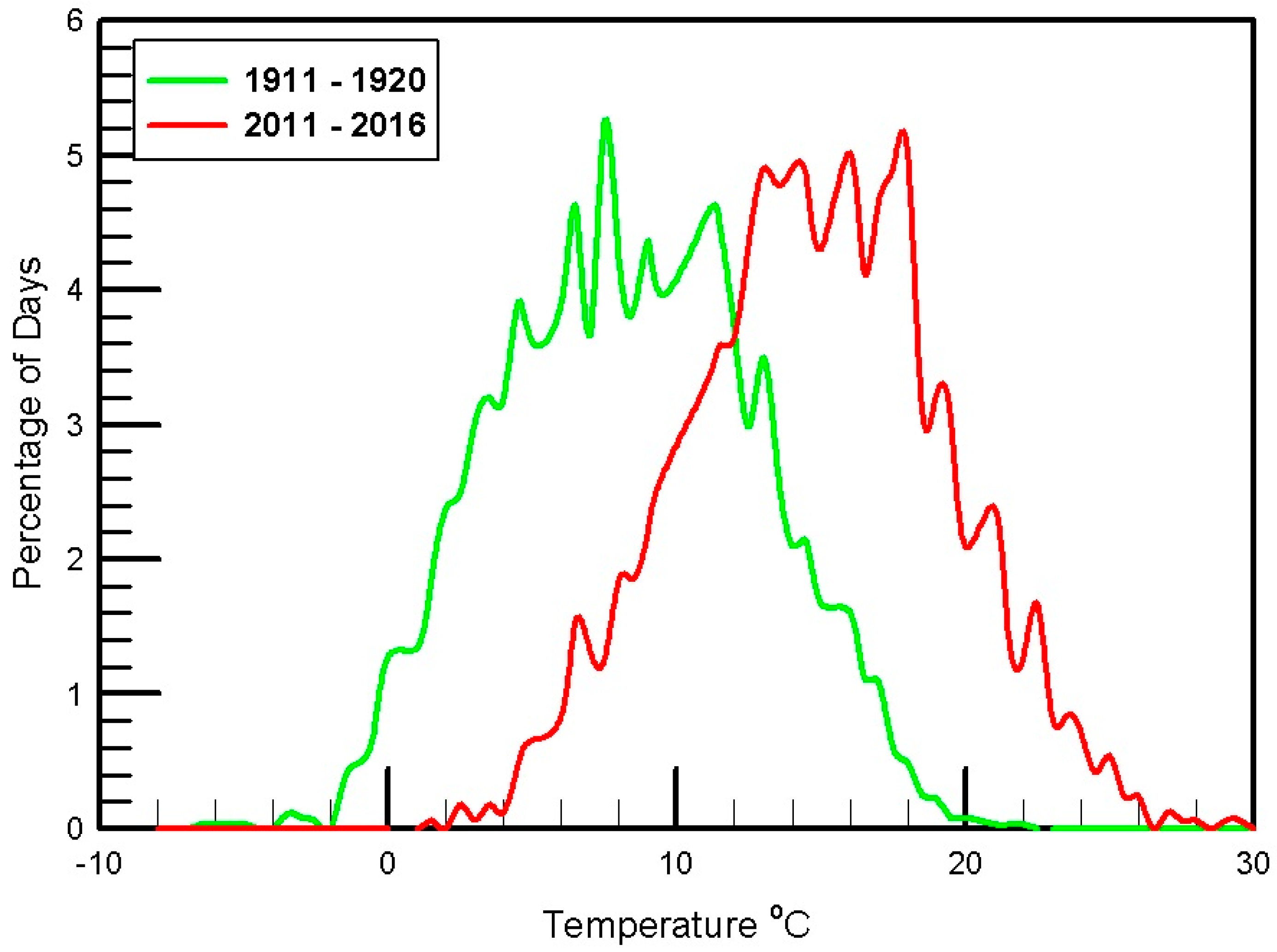
Figure 5 shows a very different pattern. The entire distribution has shifted toward higher temperatures with the frequency of colder nights changing as much as warmer nights. For example, in the 1911–1920 period, there are a substantial number of nights with a minimum temperature below 0 °C, while in the 2011–2016 period there were none at all. Similarly, in the 1911–1920 period, there were almost no nights with a temperature greater than 20 °C, but in the 2011–2016 period there were a great many. This would not suggest any sort of maximum nighttime temperature in the same way that the daytime temperature distribution does.
4.3. Rainfall
Table 4 provides a summary of the rainfall in Pasadena for the entire Study Period, the Test Period, and the Control Period for the entire year and for the months of October through April. All of the data in all of the periods examined were non-normally distributed. Table 4 provides the number of results, the mean, median, 25th percentile, 75th percentile, the number of driest and wettest months, and the results of the MWRST and FE tests. In every case except one (November), the mean, median, 25th percentile, and 75th percentile values are lower in the Test Period than the Control Period. In none of those cases was the degree of difference statistically significant, although in three cases the probability that the difference was caused by other effects was 0.2 or less—the entire year, October, and December (p-value for the November MWRST result was also less than 0.2, but the median November rainfall was higher in the Test Period as compared to the Control Period). The percent change in the median value for these three study groups was 11%, 28%, and 42%, respectively (November was 183%). March showed a 25% decrease in median rainfall between the Control and Test Periods but the p-value was 0.338. There were 23 months that were equally the driest in the Study Period for October, 15 of which were in the Test Period. Conversely, 8 of the 10 wettest Octobers were in the Control Period and the p-value for the FE test were 0.2 or less for both the wettest and driest months in October. In December, like October, 8 of the 10 wettest months occurred in the Control Period, but only five of the driest months occurred in the Control Period, which is similar to March. April showed only a small decrease in the median rain fall (7%), however of the 13 driest months, 12 occurred during the Test Period. This was a statistically significant deviation from the overall all pattern using the FET. It is important to note that the years 2011–2016 were marked by the most severe drought in California’s history [1] and three of the driest periods in April occurred in that time span.
5. Discussion
The average temperatures in Pasadena have clearly increased significantly over the Study Period. The pattern of temperature increases paralleled those seen globally, in the Northern Hemisphere, North America, and California. However, the degree of change was considerably larger in Pasadena. Pre-1950, temperatures were much lower than the baseline data and the post-1950 temperature data was much higher. Globally, the lowest difference from the Base Period data was −0.59 °C (1907) and the highest was 1.45 °C (2016), while for Pasadena, the lowest difference was −3.40 °C (1918) and the highest was 4.40 (2014). Figure 1 shows that pattern was not uniform but increased over time, with the data in Pasadena that showed the greatest divergence being at the two ends of the study period.
Daytime temperatures in Pasadena have increased significantly since records were first collected in 1885 but only for certain times of the year. This is consistent with local climatic models which predict increases in local temperatures [2]. Since nighttime temperatures are rising more rapidly than daytime temperatures, the difference between the two should be decreasing; the data on Table 2 is suggestive of this, but it is not conclusive.
This difference between June and January temperatures is likely due to the marine layer in southern California [9]. The marine layer consists of low-altitude stratus clouds that form over the Pacific Ocean coast which is then advected by on shore winds over large areas of coastal California. These clouds form a sheetlike deck which is rather uniform in depth of 500 to 2000 m and extends for large distances inland. Further inland, motion is generally prevented by the line of very high coast mountain ranges, such as the San Gabriel Mountains. It is thus not unusual for there to be many continuous days and weeks between April and June when the weather in Pasadena is cool and overcast (informally locally known as “May Gray” or “June Gloom”), although this sort of weather can occur at any time of year. The marine layers may last a few hours or an entire day but typically “burns off” by mid-afternoon [9].This greatly reduces incoming solar radiation, including both incoming incident shortwave radiation (ISR) and longwave radiation (ILR) as they are reflected back into space by the surface of the clouds. The ISR and ILR that do reach the ground are reflected or absorbed and re-emitted as outgoing shortwave radiation (OSR) and longwave radiation (OLR), with an increased ratio of longwave to shortwave radiation. Furthermore, the low cloud deck reflects both OSR and OLR back towards earth and are likewise both emitted and reflected by the earth’s surface. Greenhouse Gases (GHGs), e.g. carbon dioxide, absorb ILR and OLR but not ISR and OSR, so as the concentrations of GHGs increase, the amount of energy captured by the atmosphere increases. However, the marine layer creates a well-buffered environment which minimizes significant increases in atmospheric daytime temperatures. Nevertheless, in the winter and summer, these conditions do not prevail nearly as much because as more sunlight reaches the surface, more OLR will be emitted and less OLR will be reflected back toward the surface, so GHGs can capture more OLR hence atmospheric temperatures can increase. The marine layer has both an energy reflecting effect and an energy trapping effect. This dynamic does not occur the same way at night since there is no ISR or ILR, only OSR and OLR, and as a result, the marine layer only has an energy trapping effect but no energy reflecting effect. This explains why the nighttime temperatures have increased faster than daytime temperatures and why there is less variability between seasons at night as compared to during the daylight hours [10].
Additionally, there is the Urban Heat Island (UHI) effect [11]. Urban areas with their large masses of concrete, asphalt, steel, and glass can absorb much more heat than agricultural and rural areas. Therefore, as an area becomes more urbanized, air temperatures will increase separately from climatic changes caused by GHGs and the absorption of OLR. However, it is not very likely that the UHI effect is a major contributor to the atmospheric effects, as the location of the temperature measuring equipment has always been in a significantly urbanized area even in the 1880s. The city was largely as urbanized as it is today, especially near the measuring equipment since the 1920s. Further, as can be seen in Figure 2, Figure 3, Figure 4 and Figure 5, temperatures have increased since the 1920s when there was no appreciable increase in the degree of urbanization in Pasadena.
This change in atmospheric temperatures appears to have had some measureable impact on local rainfall. While the median rainfall declined in all months studied except November, the differences were generally not large or statistically significant, with two exceptions. The months of October and April did appear to show measurable differences in rainfall, as measured by changes in median rainfall, the frequency of extremely dry months, and extremely wet months. Most rainfall in the Pasadena area occurs in the colder months of the year, October through April, and generally arrives in the form of front storms generated in the Bering Sea thousands of kilometers to the northwest. Local climatic changes in Pasadena undoubtedly cannot have any direct impact on the pattern of storm formation and movement into southern California. However, since October and April are months characterized by the least amount of rainfall in general, the “edges” of the rainy season, as it were, it could be possible that the higher temperatures could impact smaller storm events. Pasadena is located on the windward side of the San Gabriel Mountains, creating conditions for orographic lift with associated adiabatic cooling and increasing relative humidity and vapor pressure. With smaller cold fronts, local warming may raise the temperature in the clouds, reducing vapor pressure and inhibiting droplet formation.
6. Conclusions
It is very clear that there is ACC on a local scale in the Pasadena area, since air temperatures have been increasing over the last 100 years to a measurable and statistically significant degree. Nighttime temperatures have increased much more than daytime temperatures and temperatures in the colder months have increased more than warmer months. The data suggests that there is a maximum daytime temperature of approximately 40 °C, which limits the amount of increase possible during daylight hours. It would appear that this change in air temperature may be having some limited impact on rainfall in the months of April and October.
Acknowledgments
The author would like to thank Onderdonk of the California Institute of Technology for his assistance on this paper, Robert Haw of the Jet Propulsion Laboratories, and Peter Kalmus of the University of California, Los Angeles. The author would also like to thank Diana Hsueh and Mercedes Acevedo of PWP for their assistance in the preparation of this manuscript.
Conflicts of Interest
The author declares no conflict of interest.
References
- Kimbrough, D.E. Local Climate Change in Pasadena California and the Impact on Stream Flow. J. Am. Water W. Assoc. 2017, 109, E416–E425. [Google Scholar] [CrossRef]
- Los Angeles Basin Stormwater Conservation Study. Available online: https://www.usbr.gov/lc/socal/basinstudies/LABasin.html (accessed on 12 April 2018).
- Barsugli, J.J.; Guentchev, G.; Horton, R.M.; Wood, A.; Mearns, L.O.; Liang, X.-Z.; Winkler, J.A.; Dixon, K.; Hayhoe, K.; Rood, R.B.; et al. The Practitioner’s Dilemma: How to Assess the Credibility of Downscaled Climate Projections. Eos, Trans. Am. Geophys. Union 2013, 94, 424–425. [Google Scholar] [CrossRef]
- Sun, F.; Walton, D.; Hall, A. A hybrid dynamical–statistical downscaling technique, part II: End-of-century warming projections predict a new climate state in the Los Angeles region. J. Clim. 2015, 28, 4618–4636. [Google Scholar] [CrossRef]
- Hall, A. Projecting regional change. Science 2014, 346, 1461–1462. [Google Scholar] [CrossRef] [PubMed]
- Napton, D.E. Southern and Central California Chaparral and Oak Woodlands Ecoregion. In Status and Trends of Land Change in the Western United States—1973 to 2000; Benjamin, M.S., Tamara, S.W., William, A., Eds.; U.S. Geological Survey: Reston, VA, USA, 2012. [Google Scholar]
- De Muth, J.E. Basic Statistics and Pharmaceutical Statistical Applications, 3rd ed.; CRC Press: Boca Raton, FL, USA, 2014; pp. 242–244. ISBN 9781466596733. [Google Scholar]
- National Oceanic and Atmospheric Administration. Climate at a Glance: Global Time Series. Available online: https://www.ncdc.noaa.gov/cag/ (accessed on 10 April 2018).
- Edinger, J.G. Modication of Marine Layer over Southern California. J. Appl. Meteorol. 1963, 2, 706–712. [Google Scholar] [CrossRef]
- Terjung, W.H.; O’Rourke, P.A. Influences of Physical Structures on Urban Energy Budgets. Bound. Layer Meteorol. 1980, 19, 421–439. [Google Scholar] [CrossRef]
- Hatzianastassiou, N.; Fotiadi, A.; Matsoukas, C.; Pavlakis, K.G.; Drakakis, E.; Hatzidimitriou, D.; Vardavas, I. Long-term global distribution of Earth’s shortwave radiation, budget at the top of atmosphere. Atmos. Chem. Phys. 2004, 4, 1217–1235. [Google Scholar] [CrossRef]
Figure 1.
Annual average surface temperature deviations from the 1910 to 2000 average at several locations, 1886–2016.
Figure 1.
Annual average surface temperature deviations from the 1910 to 2000 average at several locations, 1886–2016.

Figure 2.
Median daytime temperatures by decade and month, 1885–2016.

Figure 3.
Median nighttime temperatures by decade and month, 1885–2016.

Figure 4.
Frequency of daytime temperatures in Pasadena by decade, 1911–2016.

Figure 5.
Nighttime temperatures in Pasadena by decade, 1911–2016.


Table 1.
Annual average surface temperature deviations from the 1910–2000 average at several locations between 1886–2016 with the Mann-Whitney Rank Sum Test (MWRST) and Spearman Rank Order Correlation. All Results are in Degrees Centigrade Difference.
Table 1.
Annual average surface temperature deviations from the 1910–2000 average at several locations between 1886–2016 with the Mann-Whitney Rank Sum Test (MWRST) and Spearman Rank Order Correlation. All Results are in Degrees Centigrade Difference.
| Location | Period | n | Mean | 50th | 25th | 75th | MWRST | ||
|---|---|---|---|---|---|---|---|---|---|
| Percentile | U | T | p | ||||||
| Global | 1886–2016 | 131 | 0.08 | −0.03 | −0.26 | 0.27 | |||
| 1886–1949 | 64 | −0.21 | −0.21 | −0.38 | −0.03 | ||||
| 1950–2016 | 67 | 0.35 | 0.23 | −0.05 | 0.80 | 567 | 2647 | <0.001 | |
| Norther Hemisphere | 1886–2016 | 131 | 0.08 | −0.03 | −0.29 | 0.26 | |||
| 1886–1949 | 64 | −0.20 | −0.19 | −0.39 | 0.01 | ||||
| 1950–2016 | 67 | 0.35 | 0.23 | −0.05 | 0.84 | 428 | 2808 | <0.001 | |
| North America | 1910–2016 | 107 | 0.14 | 0.080 | −0.31 | 0.46 | |||
| 1886–1949 | 40 | −0.20 | −0.19 | −0.39 | 0.01 | ||||
| 1950–2016 | 67 | 0.28 | 0.24 | −0.21 | 0.64 | 871 | 1691 | 0.003 | |
| California | 1895–2016 | 122 | 0.10 | 0.03 | −0.39 | 0.50 | |||
| 1886–1949 | 55 | −0.24 | −0.28 | −0.56 | 0.00 | ||||
| 1950–2016 | 67 | 0.35 | 0.33 | 0.00 | 0.83 | 704 | 2244 | <0.001 | |
| Pasadena | 1886–2016 * | 114 | 0.29 | 0.15 | −0.80 | 1.23 | |||
| 1886–1949 * | 47 | −0.68 | −0.90 | −1.40 | 0.20 | ||||
| 1950–2016 | 67 | 0.98 | 0.80 | 0.10 | 1.80 | 457 | 1585 | <0.001 | |
| Norther Hemisphere | North America | California | Pasadena | ||||||
| Global | R | 0.99 | 0.81 | 0.69 | 0.64 | ||||
| p | <0.0001 | <0.0001 | <0.0001 | <0.0001 | |||||
| Norther Hemisphere | R | 0.84 | 0.67 | 0.59 | |||||
| p | <0.0001 | <0.0001 | <0.0001 | ||||||
| North America | R | 0.60 | 0.54 | ||||||
| p | <0.0001 | <0.0001 | |||||||
| California | R | 0.79 | |||||||
| p | <0.0001 | ||||||||
* There is a gap in the record between 1890–1893 and 1896–1908.
Table 2.
Air temperatures in Pasadena between 1886–2016
All results are in Degrees Centigrade
Daily maximum temperatures.
Table 2.
Air temperatures in Pasadena between 1886–2016
All results are in Degrees Centigrade
Daily maximum temperatures.
| Months | Period | n | Mean | 50th | 25th | 75th | % Change in Median | MWRSTU Value | Probability |
|---|---|---|---|---|---|---|---|---|---|
| All | Study | 41,890 | 25.0 | 25.0 | 20.0 | 30.0 | |||
| Control | 17,590 | 24.2 | 24.4 | 19.4 | 29.4 | ||||
| Test | 24,299 | 25.5 | 25.6 | 20.6 | 30.6 | 5 | 190,921,246 | <0.001 | |
| January | Study | 3580 | 19.1 | 18.9 | 15.6 | 22.8 | |||
| Control | 1505 | 18.1 | 17.8 | 14.4 | 22.2 | ||||
| Test | 2075 | 25.5 | 19.4 | 16.1 | 23.3 | 9 | 1,258,874 | <0.001 | |
| February | Study | 3213 | 20.0 | 19.4 | 16.1 | 23.3 | |||
| Control | 1320 | 18.6 | 18.3 | 15.0 | 21.7 | ||||
| Test | 1893 | 20.9 | 20.6 | 17.2 | 24.4 | 13 | 919,116 | <0.001 | |
| March | Study | 3225 | 21.2 | 20.6 | 17.8 | 24.4 | |||
| Control | 1458 | 20.1 | 19.4 | 16.7 | 23.3 | ||||
| Test | 2067 | 21.9 | 21.7 | 18.3 | 25.0 | 5 | 2,245,290 | <0.001 | |
| April | Study | 3377 | 23.0 | 22.8 | 19.4 | 26.7 | |||
| Control | 1380 | 22.0 | 21.7 | 18.3 | 25.6 | ||||
| Test | 1997 | 23.8 | 23.3 | 20.0 | 27.2 | 7 | 1,107,918 | <0.001 | |
| May | Study | 3514 | 24.7 | 24.4 | 21.7 | 27.8 | |||
| Control | 1452 | 23.9 | 23.3 | 20.6 | 26.7 | ||||
| Test | 2052 | 25.3 | 25.0 | 22.2 | 28.3 | 7 | 1,239,675 | <0.001 | |
| June | Study | 3378 | 27.7 | 27.8 | 25.0 | 30.6 | |||
| Control | 1410 | 27.2 | 27.2 | 24.4 | 30.0 | ||||
| Test | 1968 | 28.2 | 28.3 | 25.0 | 31.1 | 4 | 1,209,085 | <0.001 | |
| July | Study | 3558 | 31.4 | 31.1 | 29.4 | 33.3 | |||
| Control | 1492 | 31.0 | 31.1 | 28.9 | 32.8 | ||||
| Test | 2066 | 31.6 | 31.7 | 29.4 | 33.3 | 2 | 1,348,717 | <0.001 | |
| August | Study | 3612 | 31.8 | 31.7 | 29.4 | 33.9 | |||
| Control | 1549 | 31.3 | 31.1 | 28.9 | 33.9 | ||||
| Test | 2063 | 32.2 | 32.2 | 30.0 | 34.4 | 4 | 1,358,929 | <0.001 | |
| September | Study | 3500 | 30.7 | 30.6 | 27.2 | 33.9 | |||
| Control | 1500 | 29.7 | 29.4 | 26.7 | 32.8 | ||||
| Test | 2000 | 31.4 | 31.7 | 27.8 | 34.4 | 8 | 1,189,293 | <0.001 | |
| October | Study | 3587 | 27.0 | 26.7 | 23.3 | 30.6 | |||
| Control | 1519 | 25.9 | 25.6 | 22.2 | 29.4 | ||||
| Test | 2068 | 27.8 | 27.2 | 23.9 | 31.1 | 6 | 1,255,054 | <0.001 | |
| November | Study | 3387 | 23.1 | 22.8 | 19.4 | 26.7 | |||
| Control | 1525 | 23.0 | 22.8 | 19.4 | 26.7 | ||||
| Test | 1982 | 23.2 | 22.8 | 20.0 | 26.7 | 0 | 1,483,766 | 0.35 | |
| December | Study | 3563 | 19.5 | 18.9 | 16.1 | 22.8 | |||
| Control | 1519 | 19.1 | 18.9 | 15.6 | 22.8 | ||||
| Test | 2044 | 19.8 | 19.4 | 16.7 | 22.8 | 2 | 1,409,343 | <0.001 |
Table 3.
Air temperatures in Pasadena between 1886–2016
All results are in Degrees Centigrade
Daily minimum temperatures.
Table 3.
Air temperatures in Pasadena between 1886–2016
All results are in Degrees Centigrade
Daily minimum temperatures.
| Months | Period | n | Mean | 50th | 25th | 75th | % Change in Median | MWRSTU Value | Probability |
|---|---|---|---|---|---|---|---|---|---|
| All | Study | 41,856 | 10.7 | 10.6 | 10.6 | 7.20 | |||
| Control | 17,588 | 9.4 | 9.4 | 6.1 | 12.8 | ||||
| Test | 24,268 | 11.6 | 11.7 | 8.3 | 15.0 | 24 | 58,789,490 | <0.001 | |
| January | Study | 3579 | 6.0 | 6.1 | 3.9 | 8.3 | |||
| Control | 1505 | 4.6 | 4.4 | 2.2 | 6.7 | ||||
| Test | 2074 | 7.0 | 7.2 | 5.0 | 9.4 | 64 | 917,958 | <0.001 | |
| February | Study | 3213 | 6.8 | 6.7 | 4.4 | 8.9 | |||
| Control | 1320 | 5.5 | 5.6 | 3.3 | 7.8 | ||||
| Test | 1893 | 7.8 | 7.8 | 5.6 | 10.0 | 39 | 748,569 | <0.001 | |
| March | Study | 3525 | 7.9 | 7.8 | 5.6 | 10.0 | |||
| Control | 1458 | 6.8 | 6.7 | 4.4 | 8.9 | ||||
| Test | 2067 | 8.6 | 8.9 | 6.7 | 10.6 | 33 | 953,700 | <0.001 | |
| April | Study | 3372 | 9.5 | 9.4 | 7.8 | 11.7 | |||
| Control | 1380 | 8.5 | 8.9 | 6.7 | 10.6 | ||||
| Test | 1998 | 10.1 | 10.0 | 8.3 | 12.2 | 12 | 953,700 | <0.001 | |
| May | Study | 3513 | 11.4 | 11.7 | 9.4 | 13.3 | |||
| Control | 1452 | 10.3 | 10.6 | 8.3 | 12.2 | ||||
| Test | 2061 | 12.2 | 12.2 | 10.6 | 13.9 | 15 | 931,875 | <0.001 | |
| June | Study | 3377 | 13.3 | 13.3 | 11.7 | 15.0 | |||
| Control | 1410 | 12.0 | 12.2 | 10.6 | 13.9 | ||||
| Test | 1977 | 14.3 | 14.4 | 12.8 | 15.6 | 18 | 700,701 | <0.001 | |
| July | Study | 3553 | 15.6 | 15.6 | 13.9 | 17.2 | |||
| Control | 1492 | 14.3 | 14.4 | 12.8 | 16.1 | ||||
| Test | 2064 | 16.6 | 16.7 | 15.0 | 18.3 | 16 | 779,121 | <0.001 | |
| August | Study | 3598 | 15.8 | 15.6 | 13.9 | 17.8 | |||
| Control | 1549 | 14.4 | 14.4 | 12.2 | 16.1 | ||||
| Test | 2047 | 16.9 | 16.7 | 15.0 | 18.3 | 16 | 780,254 | <0.001 | |
| September | Study | 3499 | 15.0 | 14.4 | 12.5 | 16.7 | |||
| Control | 1500 | 13.1 | 12.8 | 11.1 | 15.0 | ||||
| Test | 1999 | 16.1 | 16.1 | 13.9 | 17.8 | 26 | 729,880 | <0.001 | |
| October | Study | 3584 | 12.0 | 12.2 | 10.0 | 14.4 | |||
| Control | 1519 | 10.4 | 12.2 | 10.0 | 14.4 | ||||
| Test | 2065 | 13.2 | 13.3 | 11.1 | 15.0 | 9 | 808,120 | <0.001 | |
| November | Study | 3388 | 8.54 | 8.3 | 6.1 | 11.1 | |||
| Control | 1525 | 7.48 | 7.2 | 5.0 | 9.4 | ||||
| Test | 1983 | 9.45 | 9.4 | 7.2 | 11.7 | 31 | 988,824 | <0.001 | |
| December | Study | 3561 | 6.4 | 6.1 | 4.4 | 8.3 | |||
| Control | 1519 | 5.5 | 5.6 | 3.3 | 7.8 | ||||
| Test | 2042 | 7.0 | 7.2 | 5.0 | 8.9 | 29 | 1,131,512 | <0.001 |
Table 4.
Rainfall in Pasadena between 1883 and 2016 compared by the Mann-Whitney Rank Sum Test and Fisher Exact Test.
All Results are in millimeters of rain or Number of Months.
Table 4.
Rainfall in Pasadena between 1883 and 2016 compared by the Mann-Whitney Rank Sum Test and Fisher Exact Test.
All Results are in millimeters of rain or Number of Months.
| Months | Period | Years | n | Mean | 50th | 25th | 75th | Driest Months | Wettest Months | Median MWRST | Driest FE | Wettest FE | |
|---|---|---|---|---|---|---|---|---|---|---|---|---|---|
| U | P | P | P | ||||||||||
| All | Study | 1883–2016 | 134 | 508 | 456 | 334 | 648 | 395 | 100 | ||||
| Control | 1883–1949 | 67 | 523 | 462 | 361 | 657 | 194 | 53 | |||||
| Test | 1950–2016 | 67 | 491 | 411 | 289 | 628 | 201 | 47 | 1957 | 0.202 | |||
| October | Study | 1883–2016 | 134 | 19.4 | 11.4 | 1.0 | 24.6 | 23 | 10 | ||||
| Control | 1883–1949 | 67 | 22.0 | 12.4 | 2.3 | 25.4 | 8 | 8 | |||||
| Test | 1950–2016 | 67 | 16.8 | 8.9 | 0.3 | 23.4 | 15 | 2 | 1944 | 0.181 | 0.20 | 0.20 | |
| November | Study | 1883–2016 | 134 | 43.1 | 25.5 | 4.0 | 61.6 | 14 | 10 | ||||
| Control | 1883–1949 | 67 | 38.8 | 18.5 | 3.8 | 53.1 | 8 | 6 | |||||
| Test | 1950–2016 | 67 | 47.3 | 33.8 | 4.3 | 64.8 | 6 | 4 | 1945 | 0.182 | 0.6 | 0.75 | |
| December | Study | 1883–2016 | 134 | 80.1 | 51.3 | 19.1 | 122 | 10 | 10 | ||||
| Control | 1883–1949 | 67 | 91.2 | 68.6 | 24.1 | 126 | 5 | 8 | |||||
| Test | 1950–2016 | 67 | 69.1 | 40.4 | 16.8 | 112 | 5 | 2 | 1957 | 0.201 | 1.0 | 0.18 | |
| January | Study | 1883–2016 | 134 | 105 | 73.7 | 25.0 | 156 | 10 | 10 | ||||
| Control | 1883–1949 | 67 | 101 | 75.2 | 23.6 | 159 | 5 | 5 | |||||
| Test | 1950–2016 | 67 | 110 | 72.1 | 25.7 | 152 | 5 | 5 | 2174 | 0.757 | 1.0 | 1.0 | |
| February | Study | 1883–2016 | 134 | 110 | 68.7 | 27.8 | 162 | 10 | 10 | ||||
| Control | 1883–1949 | 67 | 110 | 76.5 | 27.9 | 162 | 6 | 4 | |||||
| Test | 1950–2016 | 67 | 111 | 62.2 | 25.9 | 163 | 4 | 6 | 2162 | 0.717 | 0.75 | 0.75 | |
| March | Study | 1883–2016 | 134 | 88.1 | 60.7 | 25.3 | 122 | 10 | 10 | ||||
| Control | 1883–1949 | 67 | 96.0 | 73.9 | 24.4 | 133 | 4 | 8 | |||||
| Test | 1950–2016 | 67 | 80.6 | 55.6 | 25.9 | 112 | 6 | 2 | 2028 | 0.338 | 0.75 | 0.20 | |
| April | Study | 1883–2016 | 134 | 36.1 | 18.0 | 8.3 | 52.5 | 13 | 10 | ||||
| Control | 1883–1949 | 67 | 36.4 | 18.8 | 9.7 | 52.3 | 1 | 4 | |||||
| Test | 1950–2016 | 67 | 35.8 | 17.5 | 3.8 | 52.8 | 12 * | 6 | 2095 | 0.509 | 0.003 | 0.75 | |
* Three of these were during the drought of 2011–2016.
© 2018 by the author. Licensee MDPI, Basel, Switzerland. This article is an open access article distributed under the terms and conditions of the Creative Commons Attribution (CC BY) license (http://creativecommons.org/licenses/by/4.0/).
Share and Cite
MDPI and ACS Style
Kimbrough, D.E. Changes in Temperature and Rainfall as a Result of Local Climate Change in Pasadena, California. Hydrology 2018, 5, 25. https://doi.org/10.3390/hydrology5020025
AMA Style
Kimbrough DE. Changes in Temperature and Rainfall as a Result of Local Climate Change in Pasadena, California. Hydrology. 2018; 5(2):25. https://doi.org/10.3390/hydrology5020025
Chicago/Turabian StyleKimbrough, David Eugene. 2018. "Changes in Temperature and Rainfall as a Result of Local Climate Change in Pasadena, California" Hydrology 5, no. 2: 25. https://doi.org/10.3390/hydrology5020025
Note that from the first issue of 2016, this journal uses article numbers instead of page numbers. See further details here.