Development of Monsoonal Rainfall Intensity-Duration-Frequency (IDF) Relationship and Empirical Model for Data-Scarce Situations: The Case of the Central-Western Hills (Panchase Region) of Nepal

Abstract

Intense monsoonal rain is one of the major triggering factors of floods and mass movements in Nepal that needs to be better understood in order to reduce human and economic losses and improve infrastructure planning and design. This phenomena is better understood through intensity-duration-frequency (IDF) relationships, which is a statistical method derived from historical rainfall data. In Nepal, the use of IDF for disaster management and project design is very limited. This study explored the rainfall variability and possibility to establish IDF relationships in data-scarce situations, such as in the Central-Western hills of Nepal, one of the highest rainfall zones of the country (~4500 mm annually), which was chosen for this study. Homogeneous daily rainfall series of 8 stations, available from the government’s meteorological department, were analyzed by grouping them into hydrological years. The monsoonal daily rainfall was disaggregated to hourly synthetic series in a stochastic environment. Utilizing the historical statistical characteristics of rainfall, a disaggregation model was parameterized and implemented in HyetosMinute, software that disaggregates daily rainfall to finer time resolution. With the help of recorded daily and disaggregated hourly rainfall, reference IDF scenarios were developed adopting the Gumbel frequency factor. A mathematical model [i = a(T)/b(d)] was parameterized to model the station-specific IDF utilizing the best-fitted probability distribution function (PDF) and evaluated utilizing the reference IDF. The test statistics revealed optimal adjustment of empirical IDF parameters, required for a better statistical fit of the data. The model was calibrated, adjusting the parameters by minimizing standard error of prediction; accordingly a station-specific empirical IDF model was developed. To regionalize the IDF for ungauged locations, regional frequency analysis (RFA) based on L-moments was implemented. The heterogeneous region was divided into two homogeneous sub-regions; accordingly, regional L-moment ratios and growth curves were evaluated. Utilizing the reasonably acceptable distribution function, the regional growth curve was developed. Together with the hourly mean (extreme) precipitation and other dynamic parameters, regional empirical IDF models were developed. The adopted approach to derive station-specific and regional empirical IDF models was statistically significant and useful for obtaining extreme rainfall intensities at the given station and ungauged locations. The analysis revealed that the region contains two distinct meteorological sub-regions highly variable in rain volume and intensity.

1. Introduction

1.1. Background

Nepal has experienced numerous natural hazard events over the past resulting in enormous economic losses and thousands of causalities, compounding the country’s already high level of poverty [1,2,3,4,5]. The frequent natural and human-induced disasters are due to its fragile geomorphology, active tectonics, and unplanned human activity on steep slopes combined with climate extremes [3,4,6,7,8]. Flooding and landslides occur frequently, mostly triggered by extreme precipitation or by earthquakes, as evidenced by the 2015 Gorkha earthquake. The importance of human interventions, such as road construction, on mass movements was at best underestimated and largely neglected by researchers and authorities in Nepal [9]. Landslides are caused by a number of underlying natural and human factors including slope aspect, gradient, soil type, land cover (changes), proximity to rivers and land use (i.e., road construction, quarrying) and most often triggered by rainfall or earthquakes [8,10]. Rainfall, while critical to maintaining ecosystem services and supporting livelihoods, is thus a triggering factor that needs to be understood and managed in order to reduce impacts due to flooding and mass movements and erosion. Reducing and managing climate-induced disaster-risk (e.g., damage due to floods and landslides) relies on knowledge of the frequency and intensity of rainfall events [11]. Extreme precipitation-induced pluvial flood and shallow landslide disaster management requires the establishment of intensity-duration-frequency (IDF) relationships of extreme events in order to formulate better design guidelines for the development of infrastructure so as to reduce impacts due to disaster-risk, and save lives, property and ecosystems [12].

However, inadequate rainfall data continue to hamper the establishment of reasonable IDF relationships [13,14,15]. Researchers have realized that the design of water resources projects, the management of storm water runoff and disaster mitigation planning with scarce and insufficient data are always a challenge [13,16,17]. The situation is even more challenging in the least-developed countries such as Nepal. In Nepal, the Department of Hydrology and Meteorology (DHM) is the government organization responsible for meteorological instrumentation and maintaining the climate variable database including rainfall. DHM has reported that there is no instrumentation for measuring fine-scale rainfall (e.g., hourly, sub-hourly precipitation) nor did it develop any systematic IDF relationships for the country.

This research explored the possibility of establishing an IDF relationship in the data-scarce environment of Nepal and developed an empirical IDF model to better estimate extreme rainfall events at some fixed duration of time and recurrence interval for the Panchase region in the Central-Western Hills of Nepal, a region with one of the highest annual rainfall amounts (between 4000–5000 mm, mean = 2984.40 mm, standard deviation (SD) = 1497.60). The objectives of the study were to develop monsoon season IDF relationships for the low-resolution rainfall data recording situation followed by the development of location-specific empirical IDF models, and to demonstrate the application of IDF for ungauged locations. For this purpose, the recorded daily and disaggregated hourly rainfall series were the main data sources. Using the IDF, we can better understand the short- and long-term rainfall intensity during the monsoon season that triggers mass movements and other hazards induced by intense rainfall in this region. Furthermore, the IDF relationship can be used in water resources management and infrastructure planning and design.

1.2. Rationale

The importance of rainfall and IDF relationships in addressing extreme precipitation-induced hazards such as mass-movement has been emphasized by many researchers [18,19,20]. IDF curves are also the graphical representation that summarizes the important statistical properties of extreme precipitation events [21]. First established in 1932 by Bernard [17], IDF is a statistical relationship of the intensity, duration and frequency of rainfall derived from historical rainfall data [13,16,22]. Since then, many different sets of relationships have been constructed for different parts of the world [13,16,17,22,23,24,25].

In the literature there are several functions to establish IDF relationships (e.g., [16,22,26]). Chen [26] derived a generalized IDF relationship for any location in the United States using three basic rainfall depths (e.g., 1 h 10-year, 24 h 10-year, and 1 h 100-year rainfall depth). Baghirathan and Shaw [27] and Gert et al. [28] proposed regional IDF formulae for ungauged areas while Kothyari and Garde [29] used daily rain and two-year return period to establish the IDF relation in India. Furthermore, Koutsoyiannis et al. [22] proposed a mathematical approach to formulate IDF relationships followed by the construction of IDF curves utilizing point information of long-term historical rainfall time series in the context of geographical variability and the regionalization of the IDF model.

The concept of regional IDF relationships was executed by Yu and Chen [30] and Madsen et al. [31] who examined regression techniques, while Willems [32], Yu et al. [33] and Langousis and Veneziano [19] applied a scaling method and developed regional IDF curves. Dalrymple [34] proposed a regional frequency analysis (RFA) method for pooling various data samples, also known as the index-flood procedure in hydrology [35]. Hosking et al. [36] studied the properties of a probability-weighted moments (PWMs) method based on L-moment, and Hosking and Wallis [11] showed the application L-moments for the RFA. L-moments are an efficient tool used to detect the homogeneous regions, to select suitable regional frequency distribution, and to predict extreme precipitation quantiles at a region of interest. The IDF relationship if regionalized can minimize computational time and effort to obtain the IDF curves for areas where rainfall gauging stations are not installed.

In order to establish IDF relationships in data-scarce situations, researchers need to disaggregate commonly available daily rainfall data. They have, therefore, developed methods for utilizing historical statistical information from commonly available daily rainfall to synthetically generate fine time-resolution rainfall series [13,37,38,39,40,41,42,43,44]. Stochastic simulation tools generate fine timescale synthetic rainfall series from coarser resolution, preserving similar statistical properties [37,39,40,41,45].

Nepal as a whole is dominated by S-E monsoon [46], where topography has a considerable effect on the rainfall patterns. There are four distinct hydrological seasons: pre-monsoon (April and May: AP), monsoon (June to September: JJAS), post-monsoon (October and November: ON) and winter or dry period (December to March: DJFM) in the country [46]. The monsoonal rainfall is highly variable over the country (~1000 mm–~4500 mm) and is intense in nature where more than 80% of the annual rainfall occurs in the 4 months of the monsoon [18,47], resulting in landslides, debris flows, flooding and sedimentation, threatening livelihoods and properties in numerous ways [48].

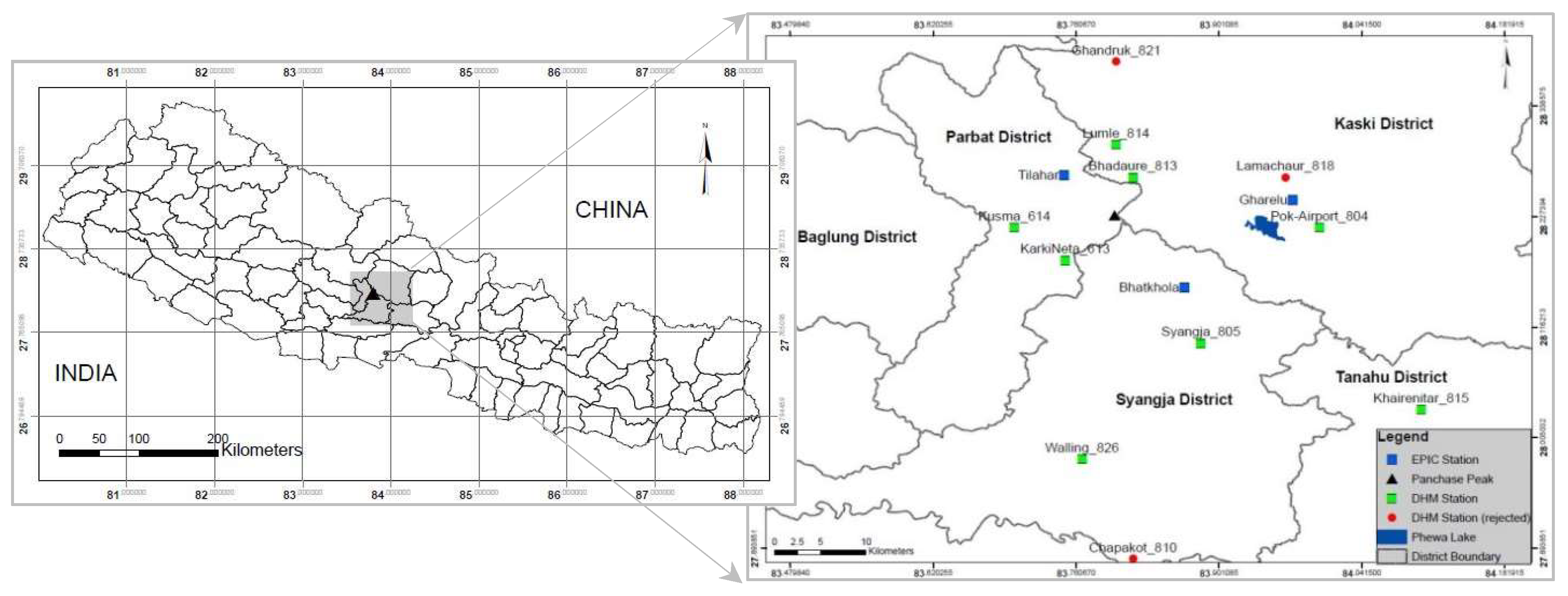
1.3. The Panchase Region

Panchase is a mountainous region in the middle-hills of Central-Western Nepal between latitudes 28°12′ N to 28°18′ N and longitudes 83°45′ E to 83°57′ E. The region is located in three districts—Kaski, Syangja and Parbat (Figure 1). The elevation varies from 742 m above sea level (masl) (outlet of Phewa Lake, near Pokhara city) to 2523 masl (Panchase Peak) and is characterized by hot, humid summers and cool-temperate winter seasons [6]. The Panchase hill range extends from the south-west to the north-west directions, dividing the region into two distinct eastern and western regions. In order to evaluate the rainfall variability and to establish the IDF relationship of the region, the historical rainfall data of 11 weather stations were collected from the DHM (

Table 1. Summery statistics of historical daily rainfall (1982–2015), missing values, and homogeneity test of all 11 stations.

Location	Department of Hydrology and Meteorology (DHM) Station Number (Nr.)	Altitude (masl)	Years of Records	Annual (mean) Rainfall (mm)	Monsoonal (mean) Rainfall (mm)	Nr. of Storms > 100 mm in 24 h	Nr. of Storms > 200 mm in 24 h	Mean (Extreme) Daily Rainfall (mm/day)	Missing Values	Homogeneity (Rejected at 95%)
GHANDRUK	821	1960	1982–2014	3384	2642	47	0	7.5	>5%	Yes
LUMLE	814	1740	1982–2014	5504	4681	352	17	15.1	<5%	No
KARKI-NETA	613	1720	1982–2014	2543	2047	56	0	7	<5%	No
BHADAURE-DEURALI	813	1600	1984–2015	3744	3093	150	7	11.3	<5%	No
LAMACHAUR	818	1070	1982–2014	4220	3380	204	10	10.5	>5%	Yes
KUSHMA	614	891	1982–2014	2531	2122	39	0	7.3	<5%	No
SYANGJA	805	868	1982–2014	2840	2280	101	7	7.8	<5%	No
POKHARA-AIRPORT	804	827	1982–2015	3969	3160	189	19	10.9	<5%	No
WALLING	826	750	1989–2012	1929	1658	61	6	5.4	<5%	No
KHAIRINITAR	815	500	1982–2012	2384	1719	50	1	6.6	<5%	No
CHAPAKOT	810	460	1982–2012	1878	1451	59	2	7.8	>5%	Yes

).

The region is one of the most studied areas in the country [48,49,50,51,52,53] due to the importance of Phewa Lake that promotes economic activities and biodiversity. However, the study of rainfall patterns, their intensity and impact have not been properly addressed yet. The Ecosystem Protecting Infrastructures and Communities (EPIC) project established and monitored three community-based rural roadside bioengineering demonstration sites in the region. In addition to capacity building and policy advocacy, the project combined formal and citizen-science by mobilizing local people and exploring local knowledge regarding climate extremes, plant species and the importance of rural access roads for building climate-resilient communities. In order to link local knowledge with formal science, the project installed three continuous recording meteorological stations in the period November–February 2014 next to each demonstration site.

2. Methods

2.1. Data Quality and Rainfall Variability

Historical daily rainfall data of 11 weather stations (Table 1 and Figure 1) in and around Panchase region with a recording period of above 30 years were obtained from DHM. Only the station in Walling had a shorter recording period of 22 years. Frequency analysis of rainfall time series requires that the data are homogeneous and independent [54]. In order to evaluate the data quality, we performed homogeneity test and evaluated for missing values. Among several methods for the homogeneity test (see [55]), we implemented simple cumulative deviations of the data from the mean according to Buishand [54] to check whether the sample data were from the same population (Equations (1)–(3), Table 1). The cumulative deviations from the mean can be expressed as:

$$S_k={\displaystyle \sum _{i=1}^k\left(X_i-\overline{X}\right)}k=1,2,\dots \dots ,n$$

(1)

where, $X_i$ are the records from the meteorological series $X_1$, $X_2$, …… $X_n$ and $\overline{X}$ is the mean. $S_{k=0}$ and $S_{k=n}$, respectively, are the initial and final value of the series.

Buishand [54] demonstrated cumulative deviations of the mean of rainfall records are often rescaled dividing $S_k$ by the sample standard deviation ($\sigma$). By evaluating the maximum (Q) or the range (R) of the rescaled cumulative deviations from the mean, the homogeneity of the data series can be tested, where:

$$Q=\underset{0\le k\le n}{\max }\left[\frac{S_k}{{\sigma }_x}\right]$$

(2)

$$R=\underset{0\le k\le n}{\max }\left(\frac{S_k}{{\sigma }_x}\right)-\underset{0\le k\le n}{\min }\left(\frac{S_k}{{\sigma }_x}\right)$$

(3)

According to Raes et al. [56] high values of Q and R indicate that data of the series are not from the same population and the fluctuations are not purely random.

The inhomogeneous data series were excluded from the analysis whereas homogeneous data series containing less than 5% missing values were further evaluated. To complete the data series, missing values were imputed using the RClimTool [57] and nearest neighborhood method as explained in XLSTAT [58].

To understand the rainfall variability in the Panchase region, we adopted a generic approach of analyzing the completed daily rainfall series in terms of the variation of annual monsoonal rain [JJAS], variation in monsoonal dry days, and extreme events of over 100 mm of rain depth in 24 h. To better estimate the variation, we grouped the rainfall series according to the hydrological year that starts from April and focused on monsoonal rainfall depth. The evaluation of historical monsoonal dry/wet days can be an indicator to understand rainfall variability, as shown by other researchers (e.g., [59]).

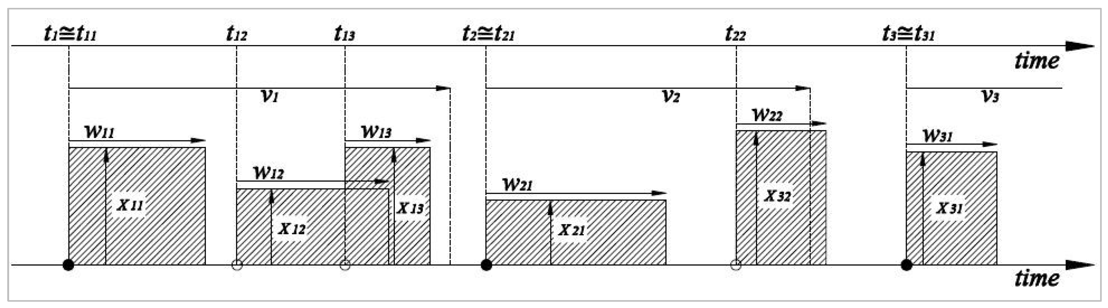
2.2. Disaggregation of Daily Rainfall

A general framework to generate synthetic rainfall time series at finer time resolution consistent with the given coarser resolution, preserving the statistical characteristics (e.g., mean, standard deviation, lag 1 auto-correlation and percentage of dry days) of both scales, was initially proposed by Koutsoyiannis [42] and Koutsoyiannis and Manetas [60]. Koutsoyiannis and Onof [44] extended the methodology to disaggregate daily rainfall into hourly data by coupling with the Bartlett–Lewis rectangular pulse (BLRP) model [41,44] with adjusting procedure [60]. The original BLRP model proposed by Rodriguez-Iturbe et al. [61] consists of five parameters ($\lambda$, $\beta$, $\gamma$, $\eta$, and ${\mu }_x$) and modelled the rainfall using rectangular pulses and characterized it by the parameters (Figure 2). The general assumption of the BLRP model as proposed by Rodriguez-Iturbe et al. [61] are:

• The occurrence of random storm events (t_i) is assumed to be modelled as a Poisson process with rate $\lambda$ and each event i is associated with a random number of cells.
• Each storm event t_ij, is assumed as a precipitation rectangular pulse with random duration t_d and the origin of storm events t_ij of each cell j occurs following a second Poisson process with rate $\beta$. The inter-arrival time of two subsequent storm events (i.e., successive cells) is independent, identically distributed and follows an exponential distribution.
• The cell-generation process terminates after time span of ${\nu }_i$ following the exponential distribution rate $\gamma$. Also, the number of cells per storm contains a geometric distribution of mean ${\mu }_c=1+\beta /\gamma$.
• The random precipitation rectangular pulse duration t_d is modelled as w_ij and also follows exponential distribution with rate $\eta$.
• Finally, the cell intensity x_ij is assumed to be exponentially distributed with mean ${\mu }_x$.

According to Rodriguez-Iturbe et al. and Onof and Wheater [62,63] the BLRP model reproduced the basic statistics but they observed difficulties in reproducing the temporal characteristics. According to Kossieris et al. [41], in order to improve the model’s flexibility in generating a greater diversity of rainfalls, Rodriguez-Iturbe et al. [63] modified the original model so that the parameter $\eta$ is randomly varied from storm to storm according to gamma distribution with a shape parameter $\alpha$ and rate parameter $\nu$ in such way that the ratios of cell origin rate ($\beta$) and storm duration rate ($\gamma$) to the parameter $\eta$ (i.e., $\kappa =\beta /\eta$ and $\varphi =\gamma /\eta$) are kept constant. Also, the parameters $\beta$ and $\gamma$ are random variables that follow a gamma distribution with common shape parameter $\alpha$ and rate parameters $\nu /\kappa$ and $\nu /\varphi$ [41]. Implementing the modified approach, the model consists of six parameters ($\lambda$, $\alpha$, $\nu$, $\kappa$, $\varphi$ and ${\mu }_x$), what we called modified BLRP (MBLRP).

The successful application of the MBLRP model in different climatic regions was reported by several researchers (e.g., [38,39,41,44,62,64,65,66,67,68,69,70,71]. The model was successfully verified and implemented through HyetosMinute, and R-based computer software by Kossieris et al. [41]. According to Kossieris et al. [41], HyetosMinute is an extended and improved version of the Hyetos model [43] to disaggregate daily rainfall depth to sub-hourly resolution [72]. HyetosMinute implements the MBLRP scheme of the Poisson-clusters model and disaggregates daily rainfall, dividing the rainfall depth into many clusters as sequences of wet days separated by at least one dry day. Also, each sequence is considered to be an independent event [39,41].

We used the HyetosMinute [72] to generate the required level of rainfall resolution according to Kossieris et al. [41]. As far as we are aware, this is the first attempt to apply a rainfall disaggregation approach in order to establish IDF relationships in Nepal and, thus, we evaluated the model parameter for each station first for the annual and second for the seasonal rainfall series. We focused on available daily monsoonal rainfall series to parameterize the model adopting a global optimization algorithm. The algorithm was implemented in a computer package called Evolutionary Annealing-Simplex (EAS) in R software [41,72] utilizing the historical statistical characteristics in terms of mean, variance, covariance, and percentage of dry days. While performing the EAS, suitable boundary conditions of the model parameters were estimated executing iterations, [41] in such a way that the model preserves the statistical characteristics of the historical rainfall.

The global optimization algorithm generated statistical parameters ($\lambda$, $\alpha$, $\nu$, $\kappa$, $\varphi$ and ${\mu }_x$) derived from the daily available monsoonal rainfall data, and rainfall depth as an input disaggregation was executed in HyetosMinute [41,72].

2.3. Evaluation of Disaggregation Model

In the case of Nepal, we are facing an inadequate data situation; hence we are limited in our ability to tune the model. We performed the model evaluation using limited fine-resolution (hourly) rainfall data recorded within the study region. We implemented the model performance evaluation scheme according to Kossieris et al. [41]. The EPIC project has established three tipping-bucket type weather stations within the test area which were calibrated to measure rainfall volume of 0.2 mm per tip with temporal resolution of an hour. Hourly rainfall data (JJAS 2016) of Gharelu, one of the test sites of EPIC, were obtained and used to evaluate the disaggregation model performance. For this purpose, we first aggregated the hourly rainfall to daily series then the series was disaggregated adopting the procedure discussed in Section 2.2. The statistical characteristics of the aggregated daily series was calculated and fitted into the EAS model to estimate the parameters (

Table 2. Estimated modified BLRP (MBLRP) parameters to be used in HyetosMinute derived from the test rainfall data series.

Location	Weather Station	$\mathit{\lambda }$ (day−1)	$\mathit{\alpha }$	$\mathit{\nu }$ (day)	$\mathit{\kappa }$	$\mathit{\varphi }$	${\mathit{\mu }}_{\mathit{x}}$ (mm/day)
Gharelu	EPIC:1	1.4805	6.9398	0.1534	1.9181	0.2615	105.98

).

We calculated the mean (E_n), variance (Var_n) and skewness (Skew_n) of the disaggregated series and compared the characteristic of aggregated series for each of the monsoonal months. Furthermore, we evaluated the recorded and disaggregated hourly intensity for the test data series for which a goodness-of-fit (GoF) test was performed.

2.4. Fitting of Probability Distribution Function and Construction of Reference Intensity-Duration-Frequency (IDF)

The probability distribution of time series with daily rainfall data is important in the field of hydrology and meteorology [73]. It is also important for the construction of IDF curves that requires the fitting of a probability distribution function (PDF) according to Koutsoyiannis et al. [22]. Several distribution models (e.g., Gumbel Extreme Value Type I (EV I), Generalized Extreme Value (GEV), Log Pearson Type III, Beta, Gamma, log-normal, Normal, etc.) are particularly useful for hydrological and meteorological time-series data analysis [22,74,75,76,77]. In Nepal there is currently limited use of IDF curves/model, and thus no preferred distribution model to be fitted for the rainfall data series. However, in some flood-frequency studies, the Gumbel Extreme Value Type I and Log-Pearson Type III were used [52]. In this research, the PDF was evaluated and the best fit was chosen for which EasyFit statistical software developed by MathWave-Technology [78] was used as employed in Gamage et al. [79] and Misic [80] and as discussed in Hosking et al. [81], Stedinger et al. [82], Koutsoyiannis [83,84] and Millington et al. [75]. The homogeneous daily rainfall data of eight weather stations discussed earlier (see Table 1) were examined by fitting the PDF, in particular GEV and EV I (Equations (4) and (5)).

$$F_x(x)=\exp \left\{-{\left[1+\kappa \left(\frac{x}{\lambda }-\psi \right)\right]}^{-\frac{1}{\kappa }}\right\}\kappa \ne 0$$

(4)

where, $\kappa >0$, $\lambda >0$ and $\psi$ are shape, scale and location parameters, respectively. For $\kappa =0$, the GEV distribution turns into the Gumbel distribution [82]:

$$F_x(x)=\exp \left[-\exp \left(-\frac{x-\psi }{\lambda }\right)\right]$$

(5)

While analyzing the daily time series we recognized that the data contain some degree of seasonality effects, leading to separation of the annual series into seasonal to better understand the rainfall characteristics. The PDF for the monsoonal daily and annual extreme time series rainfall was assessed using the test statistics adopting the Kolmogorov–Smirnov (K-S), Anderson–Darling (A-D) and chi-squared test (${\chi }^2$) as illustrated in the EasyFit software [78]. Accordingly, the best-fitted PDF was chosen and model parameters ($\kappa$, $\lambda$ and $\psi$) were estimated.

We proposed the construction of reference IDF utilizing the recorded monsoonal daily and disaggregated hourly extreme rainfall and computed the frequency of precipitation depth P_T, (in mm) for the given rainfall duration t_d (in hour) with specified return period T_r (in Years) according to Wilson [85];

$$I_T=\frac{P_T}{t_d}$$

(6)

$$P_T=P_{ave}+K_T{S}_d$$

(7)

where, $P_T$ is frequency of precipitation depth, $P_{ave}$ is mean rainfall of monsoonal annual series (recorded daily and disaggregated hourly) extremes, $S_d$ is standard deviation of annual series, and $K_T$ is Gumbel frequency factor for the given duration (Equation (8)):

$$K_T=-\frac{\sqrt{6}}{\pi }\left\{0.5772+\ln \left[\ln \left(\frac{T_r}{T_r-1}\right)\right]\right\}$$

(8)

where, T_r is return period and 0.5772 is Euler’s constant.

From Equations (6)–(8), we determined the rainfall intensities for a given duration and given return period, what we called IDF scenarios, representing given locations (i.e., stations). These IDF scenarios were later used as a reference to evaluate station-specific fine resolution IDF curves developed by implementing the mathematical model proposed by Koutsoyiannis et al. [22] expressed as below:

$$i=\frac{a\left(T\right)}{b(d)}$$

(9)

According to Koutsoyiannis et al. [22], the above expression (Equation (9)) can be expressed in terms of a(T) and b(d) as below (Equations (10) and (11)):

$$a(T)=\lambda \left\{\psi -\ln \left[-\ln \left(1-\frac{1}{T_r}\right)\right]\right\}$$

(10)

where, $\lambda$ and $\psi$ are scale and location parameters of the distribution, respectively, and $T_r$ is return period for the best-fitted PDF (i.e., EV I, see Section 3.4).

$$b(d)={(t_d+\theta )}^{\eta }$$

(11)

where, $t_d$ is duration, $\theta$ and $\eta$ are parameters to be estimated ($\theta$ > 0 and 0 < $\eta$ < 1).

In order to evaluate the PDF, three sets of parameters were derived from three different levels of analysis, respectively, from annual daily extremes, hourly extremes and monsoonal time-series rainfall depth. The main objective was to establish monsoonal IDF relationship; we focused on the monsoonal rainfall series and thus the PDF parameters. For this reason, the best-fitted PDF was adopted and we obtained $\lambda$ and $\psi$ as discussed in Section 2.4. The empirical parameter $\theta$ and $\eta$ were estimated adopting Koutsoyiannis et al. [22]. Accordingly, separate IDF curves for fine time resolution were developed representing each station. In order to estimate the performance of the mathematical model, the reference IDF curves (t_d = 1 and 24 h) were fitted to the mathematical model and results were evaluated using the standard error of prediction (SEP) (Equation (12)) and the GoF test.

$$SEP=\sqrt{\left\{\frac{{\displaystyle \sum {\left(I_s-I_p\right)}^2}}{n}\right\}}$$

(12)

where, $SEP$ is the standard error of prediction, $I_s$ and $I_p$ are, respectively, the intensities (at given duration $t_d$ and return period $T_r$) observed in the reference IDF and mathematical model predicted intensities, and $n$ is the number prediction (i.e., return periods).

In order to improve the prediction and better fitting of reference IDF, the mathematical model was calibrated, adjusting the parameter by minimizing the SEP implemented in SOLVER add-ins available in MS-EXCEL. This process of analysis and adjustment of the parameters led to the development of individual station-specific empirical models.

2.5. Estimation of IDF for Ungauged Location

Researchers have demonstrated several ways to estimate extreme storms in terms of IDF for ungauged locations. Among them logistic and multiple linear regression, spatial interpolation techniques and regional frequency analysis (RFA) are particularly in use (e.g., [11,16,22,86]). The RFA technique was initially introduced for extreme flood estimation, known as the index-flood method based on L-moments, and is also in use to estimate extreme rainfall events in the homogeneous region [11,35,82,87]. In this study, the L-moment based RFA method was used to establish regional IDF relationship and develop the regional empirical IDF model.

Details about the L-moments method can be found in Hosking and Wallis [11]. In brief, the L-moments are defined as the linear function of the probability-weighted moments (PWMs) explored by Greenwood et al. [88], with the benefit of offering a description of the shape of a probability distribution by L-skewness and L-kurtosis. The PWM can be defined as (Equation (13)):

$${\beta }_r=E\left[x{\left\{F\left(x\right)\right\}}^r\right]$$

(13)

The rth L-moment ${\lambda }_r$ is related to the rth PWM, according Hosking [89]:

$${\lambda }_{r+1}={{\displaystyle \sum _{k=0}^r{\beta }_k\left(-1\right)}}^{r-k}\left({}_k^r\right)\left({}_k^{r+k}\right)$$

(14)

Therefore, the first four L-moments are:

$$\begin{array}{l}{\lambda }_1={\beta }_0\\ {\lambda }_2=2{\beta }_1-{\beta }_0\\ {\lambda }_3=6{\beta }_2-6{\beta }_1+{\beta }_0\\ {\lambda }_4=20{\beta }_3-30{\beta }_2+12{\beta }_1-{\beta }_0\end{array}$$

The L-moments are independent of units of measurement, called L-moment ratios, and are defined to the quantities, according Hosking [89]:

$$\begin{array}{l}\tau ={\lambda }_2/{\lambda }_1\\ {\tau }_3={\lambda }_3/{\lambda }_2\\ {\tau }_4={\lambda }_4/{\lambda }_2\end{array}$$

where, $\tau$ is L-coefficient of variations (L-C_v), ${\tau }_3$ is L-coefficient of skewness (L-C_s) and ${\tau }_4$ is the L-coefficient of kurtosis (L-C_k). According to Hosking and Wallis [11], the L-moments can be defined uniquely and no two distributions can have the same L-moments.

L-moments have superior abilities to conventional moments in discriminating between different distributions, because the L-moment ratio estimators of location, scale and shape are nearly unbiased, regardless of the probability distribution from which the observations arise and efficient estimators of the characteristic of climatic data and of the parameters of the distribution. The L-moment based RFA consist of the following steps:

• Screening of data through discordancy measure;
• Identification of homogeneous regions;
• Selection of regional distribution and goodness of fit measure;
• Estimation of regional growth curve using index-flood procedure.

2.5.1. Screening of Data and Discordancy Measure

Screening of data comprises evaluation of the data in terms of gross error, homogeneity, consistency and stationarity. In addition, according to the assumptions of the index-flood method, the serial and spatial independency of sites is required. For the detection of data quality, Hosking and Wallis [11] proposed evaluation of discordancy measures D_i as an indicator for a site i. Mathematically, D_i can be expressed as (Equation (15)):

$$D_i=\frac{1}{3}{\left({\mu }_i-\overline{\mu }\right)}^T{S}^{-1}\left({\mu }_i-\overline{\mu }\right)$$

(15)

where, ${\mu }_i={\left[t^{(i)},t_3^{(i)},t_4^i\right]}^t$, $\overline{\mu }=N^{-1}{\displaystyle {\sum }_{i=1}^N{\mu }_i}$ and $S=\frac{1}{N-1}{\displaystyle {\sum }_{i=1}^N\left({\mu }_i-\overline{\mu }\right)}{\left({\mu }_i-\overline{\mu }\right)}^T$ are vectors where t, t₃ and t₄ are L-moment ratios $\overline{\mu }$ is mean of ${\mu }_i$. The measure D_i indicates how far ${\mu }_i$ is from the center of the region relative to the size of the region. Hosking and Wallis [11] recommended that the site is discordance if D_i > 3.

2.5.2. Identification of Homogeneous Region

This is the core part of RFA and based on the grouping of sites to regions in which the samples are from the same population and consist of the same frequency distributions. We implemented the L-moment based RFA by dividing the eight rain gauge stations distributed into the heterogeneous region to two homogeneous sub-regions (eastern region: Lumle, Bhadaure, Pokhara-Airport and Khairenitar; western region: Kusma, Karki-Neta, Syangja and Walling). The division was made considering the meteorological and physical characteristics such as mean annual precipitation, altitude, latitude and distance to the gauging stations to Lake Phewa. According to Hosking and Wallis [11], heterogeneity measure estimates the degree of heterogeneity in a group of sites and assesses whether they might reasonably be treated as a homogeneous region. The heterogeneity measure (Equation (16)) compares the observed and simulated dispersion of L-moments for N sites under consideration.

$$H_j=\frac{\left(V_j-{\mu }_{v_j}\right)}{{\sigma }_{v_j}},(j=1,2\mathrm{and}3)$$

(16)

The regions are regarded as “acceptably homogeneous” when H_j < 1, “possibly heterogeneous” when 1 < H_j < 2, and “definitely heterogeneous” when H_j > 2. The details of the calculation of H_j are given in Hosking and Wallis [11].

2.5.3. Selection of Regional Distribution and Goodness of Fit

L-moment ratio diagrams were constructed using the unbiased estimators of L-moments according to Hosking [89]. The curves show the theoretical relationships between L-Skewness (L-C_s) and L-Kurtosis (L-C_k) of various candidate distributions. In addition, Z-statistics (Z^DIST) defined by Hosking and Wallis [90] compare simulated L-C_s and L-C_k of fitted distribution with the regional average L-C_s and L-C_k values obtained from observed data. The following relation (Equation (17)) defines the Z^DIST:

$$Z^{DIST}=\left({\tau }_4^{DIST}-t_4^R+{\beta }_4\right)/{\sigma }_4$$

(17)

where, ${\tau }_4^{DIST}$ is the L-C_k of fitted distribution, and ${\beta }_4$ and ${\sigma }_4$ simulated regional bias and simulated regional standard deviation of $t_4^R$. The simulation was made with the fitted Kappa distribution to regional L-moments. The fit is regarded as adequate if $\left|Z^{DIST}\right|$ is close to zero and acceptable if $\left|Z^{DIST}\right|\le 1.64$ at a confidence level of 90%.

The satisfactory distributions were obtained as depicted in the $\left|Z^{DIST}\right|$ and L-moment ratio diagram. Among the satisfactory distributions, simpler distributions were chosen, and accordingly regional growth curves were developed.

2.5.4. Estimation of Regional Growth Curves using Index-Flood Procedure

The important assumption of the index-flood or the growth curves procedure was that the frequency distributions of N stations in the homogeneous region are identical apart from a site-specific scaling factor of the ith site which can be written as (Equation (18)):

$$Q_i(F)={\mu }_{i}q(F),i=1,2,\dots \dots N$$

(18)

where, $Q_i(F)$ is the precipitation at site i at a given return period, ${\mu }_i$ is the index-flood [11], N is the number of sites, and $q(F)$ is the regional growth curve, a dimensionless quantile function common to the homogeneous site. The index-flood ${\mu }_i$ also known as the scaling factor is the sample means of the data at site i. Since, we were concerned with the short duration, extreme precipitation and thus hourly (extreme) mean precipitation was considered as the index-flood (${\mu }_i=\overline{{\mu }_{i(hr)}}$). The following equations (Equations (19) and (20)) presents the regional growth curve defined by the quantile function of chosen distribution (Gen. Logistic (GLO) and GEV) for the western and eastern regions under consideration:

$$q{(F)}_{GLO}=\psi +\frac{\lambda }{\kappa }\left(1-{\left(T_r-1\right)}^{-\kappa }\right)$$

(19)

$$q{(F)}_{GEV}=\psi +\frac{\lambda }{\kappa }\left\{1-{\left[-LOG\left(1-\frac{1}{T_r}\right)\right]}^{\kappa }\right\}$$

(20)

where, $\lambda$, $\psi$ and $\kappa$ are, respectively, the scale, location and shape parameter and T_r is the return period.

Utilizing the above two regional quantile functions together with the ${\mu }_i$, we developed a nominator [a(T)] of Equation (9). For the denominator [b(d) = (t_d + θ)^η] of Equation (9), we made a use of the reference IDF and solved the following (Equation (21)) relation to obtain two parameters ($\theta$ and $\eta$) of b(d) at a given duration (t_d = 1 and 24 h) by implementing SEP (Equation (12)) as discussed in Section 2.4:

$$i=\frac{a(T)}{b(d)}=\frac{\overline{{\mu }_{i(hr)}}·q(F)}{{(t_d+\theta )}^{\eta }}$$

(21)

3. Results

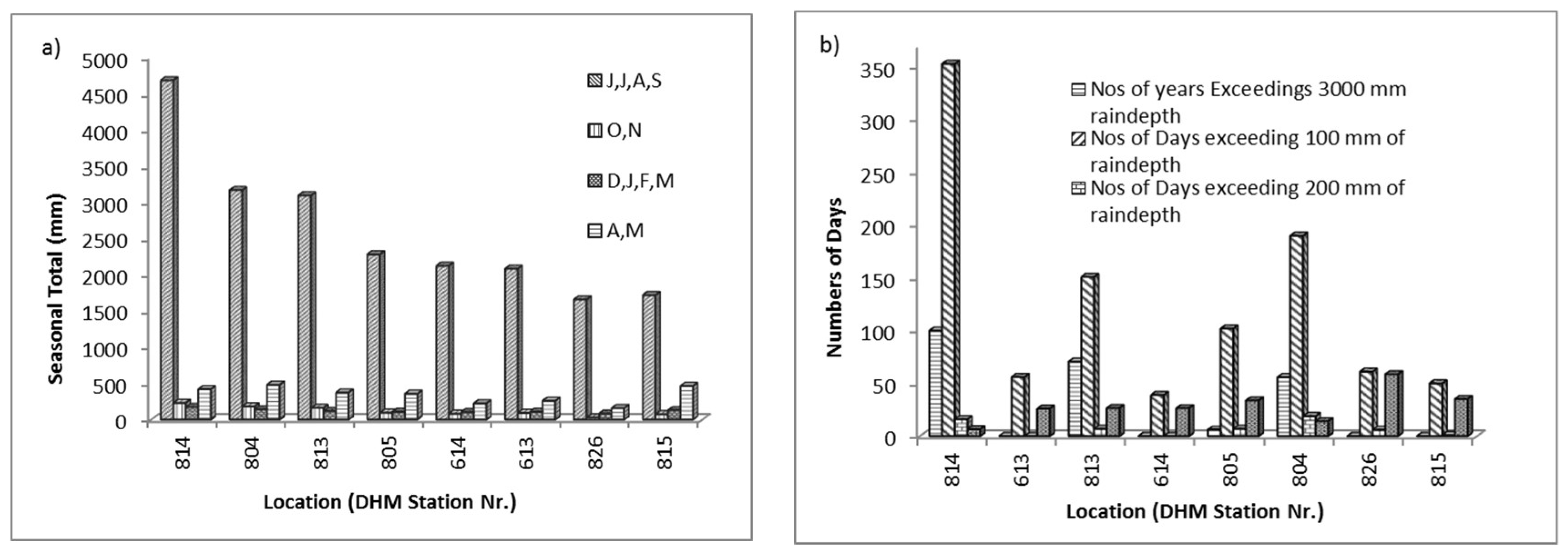
3.1. Data Quality and Rainfall Variability

The evaluation of the historical daily rainfall series from the available 11 stations led to the exclusion of three stations (Chapakot, Nr. 810; Lamachaur, Nr. 818 and Ghandruk, Nr. 821) from further analysis as these data passed the threshold of inhomogeneity or contained more than five percent of missing values. Therefore, only eight stations were considered for further analysis. Table 1 presents the characteristics of the rainfall records, with missing values and homogeneity test results.

The daily rainfall series of the eight stations showed that 81.40% of rainfall occurred during the monsoon season followed by pre-monsoon (11.10%), winter (4.0%) and post-monsoon (3.50%). Out of the eight stations, three are in the eastern part (Bhadaure-Deurali, Pokhara-Airport and Khairenitar), four in the western part (Syangja, Walling, Karki-Neta and Kusma) and Lumle on the N-W part of the Panchase hill range. The mean monsoonal rain of the eastern and western part was 2657 mm and 2027 mm, respectively. The analysis also revealed that over a 30-year period in the eight stations the total number of storms exceeding 100 mm in 24 h was 998 of which 57 exceeded 200 mm (Figure 3b). The highest recorded annual total precipitation in the region was 5631 mm in 1984 in Lumle with the mean monsoonal sum of 4681 mm (Figure 3a) and the recorded maximum rain in 24 h was 357 mm at Pokhara-Airport. This analysis clearly indicated that the rainfall in Panchase region is highly variable and the hill range distinctly divided the area into two meteorological regions.

3.2. Disaggregation of Daily Rainfall Depth

The rationale behind the rainfall disaggregation was to split the daily rainfall into hourly to sub-hourly [13,39,41,42,44,71,91] when the resolution of the available data is not fine enough. We derived MBLRP model parameters (

Table 3. Adopted MBLRP model parameters implemented in HyetosMinute derived from the historical monsoonal (daily) rainfall series of the homogeneous data set of eight stations.

SN	Location	DHM (Nr.)	$\mathit{\lambda }$ (day−1)	$\mathit{\alpha }$	$\mathit{\nu }$ (day)	$\mathit{\kappa }$	$\mathit{\varphi }$	${\mathit{\mu }}_{\mathit{x}}$ (mm/day)	Hourly (Extreme) Mean (mm/h)
1	Lumle	814	2.282	4.039	0.105	1.651	0.246	63.287	38.36
2	Karki-Neta	613	0.939	4.327	0.186	0.251	0.101	83.702	17.4
3	Bhadaure-Deurali	813	1.087	3.511	0.103	1.303	0.1493	55.347	27.89
4	Kusma	614	1.031	9.904	0.47	0.577	0.171	68.614	17.46
5	Syangja	805	0.863	5.797	0.224	1.145	0.201	68.704	18.63
6	Pokhara Airport	804	1.601	4.505	0.304	1.022	0.686	74.703	25.81
7	Walling	826	0.423	6.816	0.2	1.895	0.129	58.762	14.27
8	Khairenitar	815	0.423	6.816	0.2	1.895	0.129	58.762	13.59

) utilizing the statistical characteristics of historical monsoonal daily rainfall series for all eight stations and implemented the HyetosMinute software in R. We observed that the higher skewness value of the daily rainfall series was possibly due to strong variability in the daily rainfall time series, whereas the annual rainfall time series is rather smoothened out leading to low skewness, which was expected. The HyetosMinute effectively utilized the MBLRP model and disaggregated the monsoonal daily rainfall to synthetic hourly series even for long clusters of wet days separated by at least 1 dry day.

3.3. Evaluation of Disaggregation Model

The model discussed in Section 2.2 was evaluated utilizing the short duration hourly rainfall depth (June–September, 2016) available from the EPIC project. For this purpose, we implemented the global optimization algorithm and obtained the parameters discussed in Section 2.3 and Section 2.4 according to Kossieris et al. [41] by comparing the original and disaggregated rainfall series in terms of statistical characteristics (e.g., mean, variance and skewness). We summarized the results for each month demonstrating that the disaggregated series preserved the statistical characteristics of the recorded rainfall series (

Table 4. Comparison of statistical characteristics of recorded and disaggregated rainfall series; respectively, the mean, variance and skewness (E_n, Var_n, Skew_n and E_n′, Var_n′, Skew_n′).

Month	En	En′	Varn	Varn′	Skewn	Skewn′
June	15.41	15.41	461.53	461.52	1.644	1.644
July	46.07	46.07	2459.81	2459.79	1.105	1.105
August	28.50	28.50	1873.35	1873.36	1.831	1.831
September	45.67	45.67	1925.78	1925.77	0.966	0.966

) for the continuous weather station of the EPIC project at Gharelu in Kaski. However, we noticed the hourly synthetic rainfall series contained small differences in variance whereas the mean and skewness were similar to that of the original daily series.

In order to evaluate how well the model disaggregated the extreme intensity of the synthetic hourly rainfall depth, we compared the recorded and disaggregated extreme intensity for each of the monsoonal months. The GoF test showed that there was a good agreement among the recorded and synthetic hourly intensities of the rainfall series (${\chi }^2$ = 0.932, alpha = 0.05 and degree of freedom = 3).

3.4. Selection of Probability Distribution Function (PDF) and Parameter Estimation

The chosen PDF (EV I and GEV) were evaluated for which K-S, A-D and the chi-squared test were performed (

Table 5. Probability distribution function (PDF), estimated parameters and test statistics for the monsoonal daily time series and annual extremes.

S. N.	Location	PDF	Parameter: Monsoonal Daily Time Series			Test Statistics			Parameter: Monsoonal Annual Extremes			Test Statistics
			$\mathit{\kappa }$	$\mathit{\lambda }$	$\mathit{\psi }$	K-S	A-D	${\mathit{\chi }}^2$	$\mathit{\kappa }$	$\mathit{\lambda }$	$\mathit{\psi }$	K-S	A-D	${\mathit{\chi }}^2$
1	Lumle	GEV	0.22	18.59	23.28	0.09	41.79	161.35	0.11	183.24	28.163	0.081	0.274	1.284
		EV I	-	20.28	31.34	0.148	78.32	138.42	-	185.11	30.59	0.108	0.407	2.744
2	Karki Neta	GEV	0.37	6.84	11.26	0.137	160.39	350.25	−0.3	104.32	26.43	0.105	0.497	1.522
		EV I	-	7.67	20.97	0.229	183.24	252.72	-	101.87	21.33	0.154	0.875	0.563
3	Bhadaure Deurali	GEV	0.26	11.64	17.65	0.136	99.08	456.92	0.1	131.91	42.13	0.068	0.202	1.147
		EV I	-	12.96	25.86	0.192	115.48	187.68	-	134.16	46.13	0.08	0.254	0.214
4	Kusma	GEV	0.35	6.11	10.36	0.144	133.95	460.62	−0.3	106.06	24.33	0.101	0.377	0.313
		EV I	-	7.12	17.91	0.226	190.73	262.53	-	103.19	18.72	0.104	1.06	0.383
5	Syangja	GEV	0.45	5.12	9.83	0.178	182.59	762.43	−0.1	139.27	41.64	0.073	0.246	0.382
		EV I	-	5.59	22.6	0.278	286.99	329.4	-	139.01	36.81	0.087	0.313	0.199
6	Pokhara Airport	GEV	0.38	8.92	14.45	0.132	99.27	411.95	0.05	170.89	33.81	0.104	0.574	4.124
		EV I	-	9.87	27.62	0.238	212.39	276.32	-	171.13	36.1	0.111	0.584	4.118
7	Walling	GEV	0.61	2.05	5.47	0.326	356.66	1804.8	0.11	126.09	33.66	0.134	0.372	0.08
		EV I	-	1.3	21.29	0.323	381.37	586.36	-	127.57	37.86	0.129	0.388	0.873
8	Khairenitar	GEV	0.49	3.46	7.02	0.19	197.91	986.36	0.05	112.62	26.34	0.085	0.263	0.325
		EV I	-	3.56	18.35	0.297	318.15	520.36	-	113.45	27.68	0.088	0.277	0.643

). The K-S and A-D statistics ranked the three parameter ($\kappa$, $\psi$ and $\lambda$) GEV distribution model better over the EV I, whereas the chi-squared test ranked the two parameter ($\psi$ and $\lambda$) EV I better than the GEV.

Stedinger et al. [82] expressed that the EV I distribution is obtained when $\kappa$ = 0, and the general shape of GEV turns to EV I where $\kappa$ < 0.3. In our case, for the monsoonal annual extremes the $\kappa$ value was always less than 0.3 (Table 5) whereas this was not fully satisfied for the daily series. Also, according to Koutsoyiannis et al. [22] the performance of GEV is not very satisfactory with a small number of samples as in our case. Based on the analysis at various levels (e.g., annual and monsoonal daily series, annual extremes and disaggregated hourly extremes series), we concluded that in this case the EV I distribution was better than GEV.

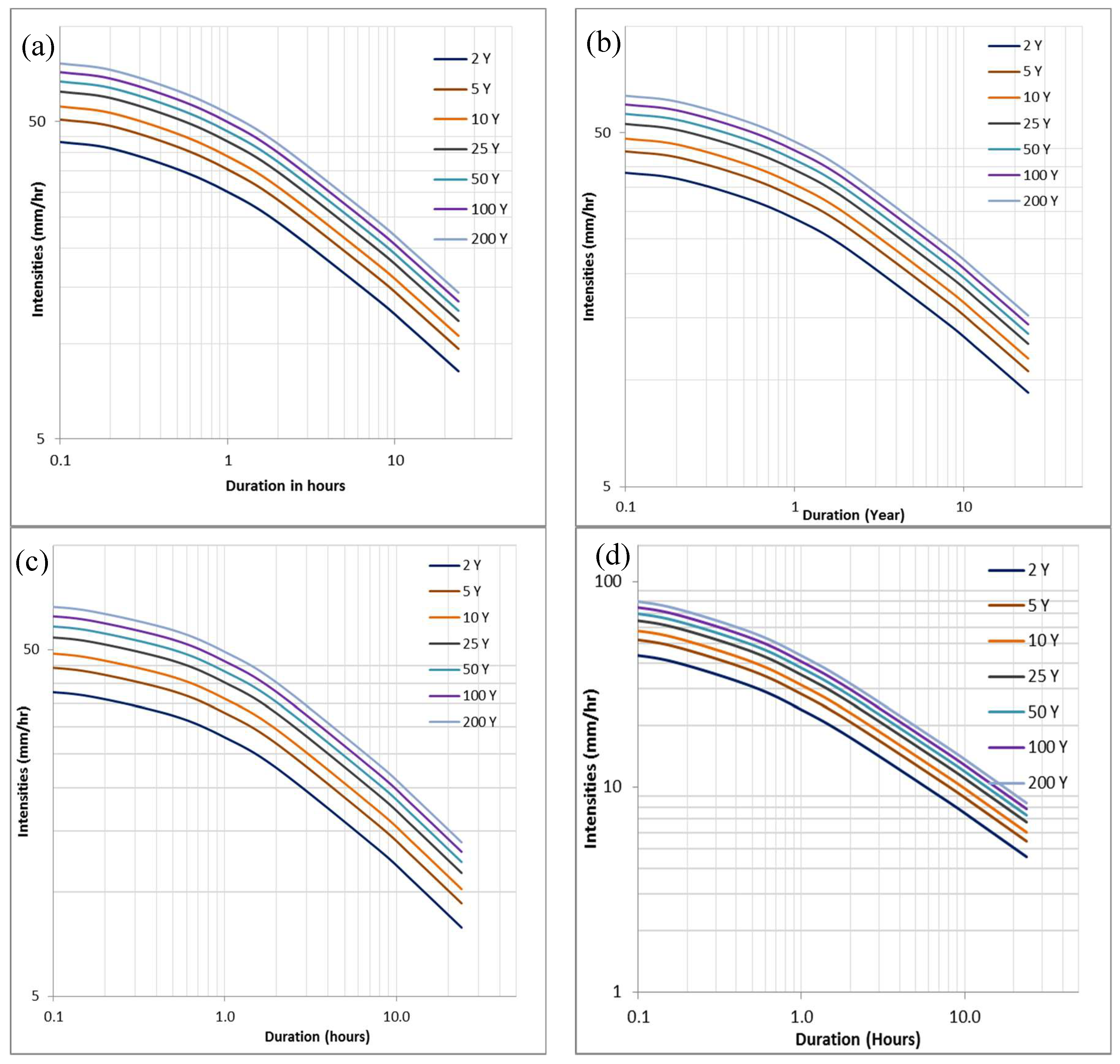
3.5. Construction of Reference and Empirical IDF Relationship

The reference IDF curves were developed for the coarser time resolution of 1 and 24 h duration utilizing the extreme rainfall from the recorded daily and disaggregated hourly monsoonal rainfall series. The frequency of extreme rainfall depth (P_T) and dimensionless Gumbel frequency factor (K_T) also known as Gumbel growth curve [92,93] were derived for the eight stations. The results showed that the frequency of precipitation is highest in the Bhadaure-Deurali station and the lowest in Khairenitar. Utilizing the method of Wilson [85], we developed the IDF curves for 1 and 24 h durations, which we called the reference IDF curves. These curves were the means to verify the finer time resolution IDF relationship.

In order to establish the IDF relationship for finer time resolution, the mathematical model proposed by Koutsoyiannis et al. [22] was parameterized. Accordingly, the best-fitted PDF parameters scale ($\lambda$) and location ($\psi$) and other empirical constants $\theta$ and $\eta$ were estimated to be fitted into the mathematical model discussed in Section 2.4. The estimated parameters are shown in

Table 6. Adopted parameters derived from Gumbel Extreme Value Type I (EV I) distribution ($\lambda$, $\psi$) and estimated ($\theta$, $\eta$) according to Koutsoyiannis et al. [22] for monsoon season rainfall time series.

SN	Location	DHM (Nr.)	$\mathit{\lambda }$	$\mathit{\psi }$	$\mathit{\theta }$	$\mathit{\eta }$
1	Lumle	814	31.335	20.284	21.889	0.943
2	Karki-Neta	613	20.97	7.673	4.226	0.959
3	Bhadaure-Deurali	813	25.857	12.961	8.428	0.988
4	Kusma	614	17.91	7.125	4.38	0.98
5	Syangja	805	22.599	5.589	5.125	0.865
6	Pokhara-Airport	804	27.623	9.866	8.977	0.957
7	Walling	826	21.292	1.298	0.99	0.5
8	Khairenitar	815	18.354	3.564	0.988	0.472

which were used to develop the station-specific mathematical IDF relationship.

3.6. Evaluation of the IDF Relationship and Development of Empirical Model

The mathematically computed IDF relationship (Section 3.5) was evaluated by fitting reference IDF scenarios, and SEP and chi-square tests were performed. The test statistics indicated that the mathematical model overestimated the IDF values for the Lumle (Nr. 814) station for both scenarios (i.e., 1 and 24 h). Similarly the Walling (Nr. 826) and Bhadaure-Deurali (Nr. 813) stations were poorly estimated for 1 h duration. The possible reason for this could be either due to the PDF that we chose or the limitation of the mathematical model where intense and prolonged rainfall occurs. This leads to the calibration of the model for which we again performed minimization of SEP by adjusting all four parameters ($\lambda$, $\psi$, $\theta$ and $\eta$) at a time. This reconstruction of the IDF significantly reduces the SEP and achieved significant test statistics except in Khairenitar station, for which both SEP and GoF were increased but yet significant.

Table 7. Standard error of prediction (SEP) and chi-square test-statistics (alpha = 0.05, test statistics = 12.59 for degree of freedom = 7) before and after the calibration of the mathematical model.

S. N.	Location	DHM Station Number (Nr.)	Before Calibration				After Calibration				Region
			Standard Error of Prediction (SEP)		Chi-Square Test Statistics (alpha at 0.05 = 12.59)		Standard Error of Prediction (SEP)		Chi-square Test Statistics (alpha at 0.05 = 12.59)
			1 h	24 h	1 h	24 h	1 h	24 h	1 h	24 h
1	Lumle	814	6.59	8.22	7.55	24.36	0.10	0.00	0.00	0.00	N-W hill range
2	Karki-Neta	613	3.19	2.10	1.81	3.55	2.05	0.00	0.72	0.00	Western part
3	Bhadaure-Deurali	813	6.10	1.95	11.47	4.00	5.70	0.56	0.17	0.05	Eastern part
4	Kusma	614	0.77	0.28	0.14	0.09	0.29	0.00	0.02	0.00	Western part
5	Syangja	805	1.27	0.52	0.24	0.21	0.00	0.87	0.00	0.60	Western part
6	Pokhara-Airport	804	1.37	1.21	0.36	0.97	0.60	0.90	0.06	0.55	Eastern part
7	Walling	826	9.27	2.21	17.41	3.05	0.87	1.10	0.19	1.02	Western part
8	Khairenitar	815	4.98	0.44	3.96	0.14	0.64	0.63	6.55	8.77	Eastern part

compared the test statistics before and after the calibration of the mathematical model. Utilizing the calibrated empirical constant (${\lambda }^{\prime }$, ${\psi }^{\prime }$, ${\theta }^{\prime }$, ${\eta }^{\prime }$) and fitting them into Equations (9)–(11), we developed the station-specific empirical IDF model.

Interpretation of the IDF relationship indicated that the eastern part generally received higher rain than the western part. Variability was also observed in the rainfall intensity from east to west. Figure 4 shows computed IDF relationship of four stations (Lumle, Pokhara-Airport, Syangja and Kusma) from the equations shown in

Table 8. Station-specific empirical model based on adjusted parameters (${\lambda }^{\prime }$, ${\psi }^{\prime }$, ${\theta }^{\prime }$, ${\eta }^{\prime }$).

S. N.	Location	DHM Nr.	Empirical Model
1	Khairenitar	815	$i=5.469\frac{7.047-\ln \left[-\ln \left(1-\raisebox{1ex}{$1$}\!\left/ \!\raisebox{-1ex}{$T_r$}\right.\right)\right]}{{\left(t_d+0.988\right)}^{0.472}}$
2	Pokhara Airport	804	$i=4.935\frac{7.21-\ln \left[-\ln \left(1-\raisebox{1ex}{$1$}\!\left/ \!\raisebox{-1ex}{$T_r$}\right.\right)\right]}{{\left(t_d+0.85\right)}^{0.434}}$
3	Bhadaure-Deurali	813	$i=5.953\frac{5.77-\ln \left[-\ln \left(1-\raisebox{1ex}{$1$}\!\left/ \!\raisebox{-1ex}{$T_r$}\right.\right)\right]}{{\left(t_d+0.867\right)}^{0.465}}$
4	Lumle	814	$i=6.197\frac{6.05-\ln \left[-\ln \left(1-\raisebox{1ex}{$1$}\!\left/ \!\raisebox{-1ex}{$T_r$}\right.\right)\right]}{{\left(t_d+0.764\right)}^{0.493}}$
5	Kusma	614	$i=4.827\frac{5.568-\ln \left[-\ln \left(1-\raisebox{1ex}{$1$}\!\left/ \!\raisebox{-1ex}{$T_r$}\right.\right)\right]}{{\left(t_d+0.378\right)}^{0.574}}$
6	Karki-neta	613	$i=7.003\frac{4.775-\ln \left[-\ln \left(1-\raisebox{1ex}{$1$}\!\left/ \!\raisebox{-1ex}{$T_r$}\right.\right)\right]}{{\left(t_d+0.311\right)}^{0.647}}$
7	Syangja	805	$i=6.122\frac{6.09-\ln \left[-\ln \left(1-\raisebox{1ex}{$1$}\!\left/ \!\raisebox{-1ex}{$T_r$}\right.\right)\right]}{{\left(t_d+0.998\right)}^{0.501}}$
8	Walling	826	$i=5.096\frac{6.093-\ln \left[-\ln \left(1-\raisebox{1ex}{$1$}\!\left/ \!\raisebox{-1ex}{$T_r$}\right.\right)\right]}{{\left(t_d+0.99\right)}^{0.5}}$

.

The basis of this IDF relationship was the theoretical probabilistic approach of the rainfall data distribution to compute the parameters of a(T) and the optimization procedure for the parameters of b(d) that represent the dynamics of the rainfall pattern discussed in Section 2.4 and demonstrated in Koutsoyiannis et al. [22]. However, there was some adjustment on the empirical constants that demonstrated better statistical significance and let the IDF curves pass through or much closer to the reference IDF point at given t_d and T_r. The reason for such an adjustment was also explained in Koutsoyiannis et al. [22] and Van de Vyver and Demaree [17] who stated that empirical considerations are not always consistent with the theoretical probabilistic approach of the IDF relationship.

3.7. Reganalization of IDF for Ungauged Locations

We executed RFA based on L-moments for the heterogeneous regions divided into two homogeneous regions (eastern region: Lumle, Pokhara-Airport, Bhadaure-Deurali and Khairenitar and western region: Kusma, Karki-Neta, Syangja and Walling) for which the heterogeneity measure was evaluated. The heterogeneity measure of the L-moment demonstrated that the sub-regions were found to be statistically homogeneous. The estimated heterogeneity measures (H) for the eastern and western regions were −0.97 and 0.34 respectively. Similarly, the L-moment ratio diagram and Z^DIST demonstrated reasonably acceptable regional distribution functions (

Table 9. List of evaluated distribution indicating the goodness-of-fit (GoF) test statistics (Z^DIST < 1.64 to accept the distribution).

S. N.	Distribution	ZDIST-Statistics/GoF		Remarks
		Eastern Region	Western Region
1	Pearson Type III	−0.19	−1.31	accept
2	Gen. Normal	0.35	−1.10	accept
3	Gaucho	−0.48	−2.37	accept/reject
4	Gen. Extreme Value	0.61	−1.12	accept
5	Gen. Logistic	1.6	0.11	accept
6	Gen. Pareto	−1.66	−3.67	reject

and Figure 5).

For the development of the regional growth curve, we chose one set up based on simple but statistically acceptable distributions, (1) Gen. Extreme Value (GEV) and (2) Gen. Logistic (GLO) respectively for the eastern and western region. Utilizing the empirical parameters (

Table 10. Chosen distribution for their fitted and estimated empirical parameters.

S. N.	Distribution	Parameters			$\mathit{\theta }$	$\mathit{\eta }$	Region
		Location ($\mathit{\psi }$)	Scale ($\mathit{\lambda }$)	Shape ($\mathit{\kappa }$)
1	Gen. Logistics (GLO)	0.98	0.388	−0.085	0.09	0.39	western
2	Gen. Extreme Value (GEV)	0.877	0.191	−0.06126	0.51	0.40	eastern

), the quantile function (Equations (19) and (20)) of the chosen distribution, and hourly (extreme) mean precipitation (see Table 3) as an index-flood, we established the IDF relation for an hour (t_d = 1 h) and a given return period (T_r = 2, 5, 10, 25, 50, 100, 200 years).

By solving Equation (21) and from the regional distribution we obtained the regional parameters shown in Table 10. We then evaluated the regional IDF with the station-specific reference IDF for the given duration (t_d = 1 and 24 h) and return period (T_r = 2, 5, 10, 25, 50, 100 and 200 years) for which SEP and GOF were performed. The test depicted that the stations Khairenitar (Nr. 815), Lumle (Nr. 814) and Walling (Nr. 826) demonstrated insignificant IDF values (i.e., the regional model either overestimated or underestimated the IDF at the given duration (t_d = 1 h and 24 h)), indicating the existence of some degree of heterogeneity, leading to the adjustment/calibration in the empirical parameters in Table 10. In

Table 11. Standard error of prediction (SEP) and chi-square test-statistics (alpha = 0.05, test statistics = 12.59 for degree of freedom = 7) before and after the calibration of the regional model.

S. N.	Location	DHM Station Number (Nr.)	Before Calibration				After Calibration				Region
			Standard Error of Prediction (SEP)		Chi-square Test Statistics (alpha at 0.05 = 12.59)		Standard Error of Prediction (SEP)		Chi-Square Test Statistics (alpha at 0.05 = 12.59)
			1 h	24 h	1 h	24 h	1 h	24 h	1 h	24 h
1	Khairenitar	815	117.6	24.8	0	0	8.69	1.11	0.19	0.98	eastern
2	Pokhara- Airport	804	1.53	0.37	0.95	0.99	no adjustment				eastern
3	Bhadaure-Deurali	813	6.1	1.95	11.47	4					eastern
4	Lumle	814	37.15	17.43	0	0.01	9.34	0.11	0.16	0.99	eastern
5	Syangja	805	1.27	0.52	0.24	0.84	no adjustment				western
6	Kusma	614	1.37	1.21	0.36	0.86					western
7	Karki-Neta	613	9.27	2.21	17.41	0.85					western
8	Walling	826	37.54	8.52	0	0.20	24.60	3.60	0	0.73	western

, we present the test statistics before and after the adjustment.

The test statistics showed that the two homogeneous sub-regions (eastern and western) can be divided into further sub-regions such as three sub-regions in the eastern region [eastern sub-region 1: Khairenitar, eastern sub-region 2: Pokhara-Airport and Bhadaure-Deurali and eastern sub-region 3: Lumle] and two in the western region [western sub-region 1: Kusma, Karki-Neta and Syangja and western sub-region and 2: Walling]. Utilizing the best-fitted regional distribution and parameters, we developed regional IDF formula for the region, as shown in

Table 12. L-moment based regional empirical IDF model for the Panchase region.

S. N.	Area (Distribution)	DHM Nr.	Empirical Model	Region/Sub-Region
1	Khairenitar (GEV)	815	$i=\frac{0.95-9.2\left\{1-{\left[-LOG\left(1-\frac{1}{T_r}\right)\right]}^{-0.05}\right\}}{{\left(t_d+0.34\right)}^{0.41}}·\overline{{\mu }_{hr}}$	eastern-1
2	Pokhara Airport & Bhadaure-Deurali (GEV)	804/813	$i=\frac{0.95-3.06\left\{1-{\left[-LOG\left(1-\frac{1}{T_r}\right)\right]}^{-0.062}\right\}}{{\left(t_d+0.5\right)}^{0.4}}·\overline{{\mu }_{hr}}$	eastern-2
3	Lumle (GEV)	814	$i=\frac{0.88-3.06\left\{1-{\left[-LOG\left(1-\frac{1}{T_r}\right)\right]}^{-0.062}\right\}}{{\left(t_d+0.9\right)}^{0.55}}·\overline{{\mu }_{hr}}$	eastern-3
4	Kusma/Karki-Neta & Syangja (GLO)	614/613/805	$i=\frac{0.98-4.47\left[1-{\left(T_r-1\right)}^{-0.085}\right]}{{(t_d+0.09)}^{0.39}}·\overline{{\mu }_{hr}}$	western-1
5	Walling (GLO)	826	$i=\frac{0.99-14.86\left[1-{\left(T_r-1\right)}^{-0.035}\right]}{{(t_d+0.01)}^{0.35}}·\overline{{\mu }_{hr}}$	western-2

t_d = duration in hour, T_r = return period in year and ${\overline{\mu }}_{hr}$ = hourly (extreme) mean precipitation.

.

The adjustment of the empirical parameters helps to improve the test statistics except for Walling, indicating that the distribution we chose was not feasible for the western sub-region2. However, we could still say that the regional empirical model is useful in evaluating the IDF of rainfall for other sub-regions.

3.8. Rainfall Intensity in the Region

The computed rainfall intensity of eastern sub-region-3 was found to be the highest in terms of shorter duration rainfall (i.e., t_d = 0.5, 1 and 2 h), whereas for the longer duration (i.e., t_d = 24 h) the rainfall was relatively intense in western sub-region 2 followed by eastern sub-region 2 and western sub-region 2. Overall, rainfall in eastern sub-region 2 was less intense followed by western sub-region 2 for the shorter duration and return periods.

Table 13. Example of computed rainfall intensity (mm/h) for some durations and return periods of regions/sub-regions.

Return Period (Tr in Year)	Duration (td in h)				Region/Sub-Region
	0.5	1	2	24
5	31.61	26.10	20.77	7.95	eastern-1
25	45.48	37.56	29.88	11.44
100	57.85	47.77	38.01	14.55
5	28.89	24.57	20.03	8.04	eastern-2
25	45.40	38.60	31.47	12.63
100	54.70	46.51	37.92	15.22
5	43.28	36.59	29.00	8.89	eastern-3
25	55.90	47.25	37.45	11.48
100	67.35	56.93	45.12	13.83
5	32.88	25.88	20.08	7.74	western-1
25	50.56	39.79	30.87	11.90
100	66.57	52.40	40.65	15.67
5	29.74	23.41	18.40	7.72	western-2
25	47.10	37.08	29.14	12.23
100	61.62	48.51	38.13	16.01

presents the computed rainfall intensity of some important return periods (T_r) and duration (t_d) for example.

4. Discussion

Geographically, the Panchase region can be divided into two sub-regions, eastern and western parts, where the Panchase hill range is sitting in the midway extending N-W to S-E direction. This study demonstrated that the region can also divide into two parts in terms of rainfall variability. Monsoonal rainfall over the region is highly variable where the eastern part (i.e., Kaski District) received higher rain (>3000 mm, except Kahirenitar) than the western part (i.e., Syangja and Parbat Districts), where mean monsoonal rainfall was below 2300 mm. The geographical setting of the eastern part is relatively wider in comparison to the western part, which is a valley containing several lakes (e.g., Phewa Lake, Begnas Lake and Rupa Lake, etc.). Rainfall is a complex process and the complexity is compounded due to the presence of lakes and high mountain topography. This complex process requires more detailed analysis considering wind direction; variation in daily temperature, solar radiation, etc. in order to better understand the rainfall variability.

Use of the historical characteristics of the recorded daily rainfall to parametrize the disaggregation model in order to generate finer resolution synthetic rainfall series is an important step forward for data-scarce regions [15,39,41,45]. The method is useful especially for those locations where fine time-resolution rainfall data is not available, leading to better estimation of the finer resolution rainfall up to a minute [41]. However, we performed the disaggregation procedure only for time periods of one hour or more since the possible error accumulation for finer resolution disaggregation is yet to be known, and has to be investigated (Kossieris, 2017:personal communication).

Although many studies (e.g., [15,37,39,40,41,42,44,45,64,94,95] have reported on the generation of synthetic rainfall series and their effectiveness, we noticed that the attention is less on the intensities. We observed that the synthetic rainfall intensities were unable to represent the recorded data of a particular day since the model implements a Poisson process and assumed that the intensity varies exponentially. In our case, however, the statistics suggest that the synthetic intensities were statistically significant for the monsoonal months and useful for developing reference IDF scenarios for the study region. In order to better understand the synthetic rainfall intensities, a rigorous analysis is required where long-term fine-resolution time-series rainfall data are available.

The application of the Gumbel frequency factor technique is popular for evaluating frequencies of rain and flood storms [92,93,96,97]. The technique is also frequently used to establish IDF relationships [22,93] using fine-resolution rainfall data [22]. In our case, due to inadequate data resolution we demonstrated the use of synthetic rainfall intensities and developed reference IDF curves utilizing the technique of Gumbel frequency factor as scenarios to be fitted into the mathematically-derived empirical IDF model for better performance. In the literature, the use of scenario IDF computed from the disaggregated and recorded rainfall extremes to establish IDF relationship is limited. This is also the case for the approach of parameter adjustment in developing IDF relationships.

The L-moment based RFA method implemented in this study was able to demonstrate that the study area is heterogeneous in terms of geography and meteorology, which we observed while constructing the station-specific IDF through Gumbel. This has led to the division of the study area into sub-regions for the RFA. Application of L-moment ratios and other statistics in identifying reasonably acceptable distributions of the data set is robust, as was depicted in the results. Therefore, the technique is useful to better understand the IDF at the ungauged locations and can save computational time and resources. In this study, we observed that while fitting the regional IDF to the reference IDF, the chosen distribution slightly underestimated the intensity for the shorter duration and return periods. However, in most cases the result was statistically significant and useful.

The present study indicated that the Panchase region is highly variable in terms of rainfall amount and intensity. Short duration and intense monsoonal rain may have different effects on floods and landslides than less intense but extended duration monsoonal rainfall, respectively noticed in the western and eastern sub-regions of the area.

This research was carried out with limited data sources in terms of resolution, length of rainfall records and sparse observational network, which is common in the country. The low-resolution rainfall data leads to an exploration of alternative approaches of disaggregation to generate synthetic hourly rainfall. For this reason, the empirical model we proposed for the region shall be used with caution. Continuous monitoring and recording of finer resolution (e.g., hourly/sub-hourly) rainfall is important in helping to improve the IDF relationship by improving storm water management. Also, in order to better understand the regional rainfall trend, non-stationary modelling will be executed and, accordingly, the regional IDF curves will be developed.

5. Conclusions

This work demonstrated monsoonal rainfall variability over a geographic region in the Central-Western hills of Nepal and attempted to establish monsoon season IDF relationships where fine-resolution rainfall data was scarce, common to many developing countries. The reported methodology and available tools are useful and applicable for ungauged locations within the study region.

The available daily data were evaluated by grouping them in subsets according to the hydrological year. This approach was helpful to better understand the rainfall variability and better fitting of PDFs, as there was a strong seasonal effect on the rainfall in the region where more than 80% of rain occurred in the four monsoonal months. The Panchase hill geographically divides the region into an eastern (i.e., Kaski District) and western (i.e., Parbat and Syangja Districts) sub-regions. Analysis of the above 30 years of homogeneous daily rainfall of eight stations in the region showed that the monsoonal rainfall amount was higher in the eastern part than was recorded in the western part. Also, the numbers of monsoonal dry days were found to be increased over the period of 30 years in the eastern part, with the constant amount of monsoonal rain indicating that the rainfall intensity is increased; whereas in the western part no clear trend was noticed in the annual monsoonal rainfall amount except in Syangja, where dry days are decreased with an increased number of storms. However, because of geographical complexity, in order to better understand the complex rainfall process in the region more detailed analysis is needed.

The proposed methodology to develop the IDF relationship and empirical model in a data-scare situation was found to be statistically significant, for which the available daily data were disaggregated to hourly synthetic series. The recorded daily and disaggregated hourly rainfall data were useful for computing the reference IDF for all the stations. The reference IDF was effective in evaluating the mathematically computed station-specific IDF relationships. The mathematical model parameters ($\lambda$, $\psi$, $\theta$ and $\eta$) were estimated according to the established methods demonstrated by other researchers (e.g., [22]). Moreover, the adjustment of the empirical constants performed better statistical significance of the IDF and demonstrated the usefulness of the model for the ungauged locations within the region. To regionalize the IDF relationships, the adopted L-moment based RFA method was implemented, dividing the region into two sub-regions first; later it was noticed that the region contains some degree of heterogeneity, leading to the production of five sets of empirical models. The models were used to estimate the regional IDF for the given duration and return periods. Although the regional models underestimated the rainfall intensity for the shorter duration and return periods while fitting them into the reference IDF, they were significant in most cases. This procedure can be extended for larger areas to establish the IDF relationship in the data-scarce situation of Nepal, leading to better management of storm water, roadside drainage design, management and the mitigation of various hazards-risks induced by mass movement.

The station-specific (Gumbel) empirical IDF model demonstrated that the short duration (i.e., 5, 10, 30, 60 min) rainfall intensity in the western part was higher than in the eastern part (highest in Karki-Neta) whereas this was not the case in the regional IDF model. The regional model revealed that the eastern sub-region 2 (Lumle area) received the intense rain. The reason behind the different intensities could be the chosen distribution model. In addition, the regional empirical IDF model generalized the distribution model to be fitted for the region and used the regional mean (extreme) precipitation leading to variation in the intensities that come from the station-specific IDF model. The interpretation of the IDF clearly indicated that the Panchase hill range distinctly divides the region into two meteorological regions. The variability of the rainfall in terms of rain volume and intensity may have different effects on mass movement, soil erosion and floods in the region, which have to be investigated for better and effective hazard-risk management.

References

1. ADPC. Nepal Hazard Risk Assessment, Part 1; Asian Disaster Preparedness Center (ADPC): Bangkok, Thailand, 2010; p. 114. [Google Scholar]
2. MoHA; DPNeT. Nepal Disaster Report 2015; DPNeT: Kathmandu, Nepal, 2015; p. 147. [Google Scholar]
3. MoENV. National Adaptation Porgramme of Action (NAPA); Ministry of Environment: Kathmandu, Nepal, 2010; p. 165.
4. Petley, D.N.; Hearn, G.J.; Hart, A.; Rosser, N.; Dunning, S.; Oven, K.; Mitchell, W. Trends in Landslide occurrence in Nepal. Nat. Hazards 2007, 43, 23–44. [Google Scholar] [CrossRef]
5. Petley, D.N. On the impact of climate change and population growth on the occurrence of landslides in Asia. Q. J. Eng. Geol. Hydrogeol. 2010, 43, 487–496. [Google Scholar] [CrossRef]
6. CBS. Compendium of Environment Statistics of Nepal 2015; Government of Nepal: Kathmandu, Nepal, 2015; p. 176.
7. Haigh, M.; Rawat, J.S. Landslide causes: Human impacts on a Himalayan landslide swarm, Belgeo. Rev. Balge Geogr. 2011, 201–220. [Google Scholar] [CrossRef]
8. Cruden, D.M.; Varnes, D.J. Landslide Types and Processes. In Landslide: Investigation and Mitigation; Transportation Research Board: Denver, CO, USA, 1996; Volume 247, pp. 36–75. [Google Scholar]
9. Sudmeier-Rieux, K.; Jaquet, S.; Derron, M.-H.; Jaboyedoff, M.; Devkota, S. A Case Study of Landslides and Coping Strategies in Two Villages of Central-Eastern Nepal. J. Appl. Geogr. 2011, 32, 680–690. [Google Scholar] [CrossRef]
10. Jaboyedoff, M.; Derron, M.H.; Voumard, J.; Leibundgut, G.; Sudmeier-Rieux, K.; Nadim, F.; Leroi, E. Human-Induced Landslides: Toward the Analysis of Anthropogenic Changes of the Slope Environment; CRC Press: Bocaton, FL, USA, 2016. [Google Scholar]
11. Hosking, J.R.M.; Wallis, J.R. Regional Frequency Analysis: An Approach Based on L-Moments; Cambridge University Press: New York, NY, USA, 1997. [Google Scholar]
12. Rakhecha, P.R.; Singh, V.P. Applied Hydrometeorology; Springer: Dordrecht, The Netherlands; Capital Publishing Company: New Delhi, India, 2009. [Google Scholar]
13. Rana, A.; Bengtsson, L.; Jothiprakash, V. Development of IDF-curves for tropical India by random cascade modelling. Hydrol. Earth Syst. Sci. Discuss. 2013, 10, 4709–4738. [Google Scholar] [CrossRef]
14. WMO-UNESCO-IAHS. Design of Water Resources Projects with inadequate data. In Proceedings of the Madrid Symposium, Madrid, Spain, 4–6 June 1973. [Google Scholar]
15. Ganguli, P.; Paulin, C. Does nonstationarity in rainfall require nonstationary intensity–duration–frequency curves? Hydrol. Earth Syst. Sci. 2017, 21, 6461. [Google Scholar] [CrossRef]
16. Nhat, L.M.; Tachikawa, Y.; Taka, K. Establishment of Intensity-Duration-frequency Curves for Precipitaiton in the Monsoon area of Vietnam. Ann. Disaster Prev. Res. 2006, 49, 93–103. [Google Scholar]
17. Van de Vyver, H.; Demaree, G.R. Construction of Intensity-Duration-frequency (IDF) curves for precipitation at Lubumabashi, Congo, under the hypothesis of inadequate data. Hydrol. Sci. J. 2010, 55, 555–564. [Google Scholar] [CrossRef]
18. Dahal, R.K.; Hasegawa, S. Representative rainfall thresholds for landslides in the Nepal Himalayas. Geomorphology 2008, 100, 429–443. [Google Scholar] [CrossRef]
19. Langousis, A.; Veneziano, D. Intensity-Duration-frequency curves from scaling representation of rainfall. Water Resour. Res. 2007, 43. [Google Scholar] [CrossRef]
20. Van Asch, T.W.J.; Buma, J.; Van Beek, L.P.H. A view on some hydrological triggering system in landslides. Geomorphology 1999, 30, 25–32. [Google Scholar] [CrossRef]
21. Gerold, L.A.; Watkins, D.W. Short Duration Rainfall Frequency Analysis in Michigan Using Scale-Invariance Assumptions. J. Hydrol. Eng. 2005, 10, 450–457. [Google Scholar] [CrossRef]
22. Koutsoyiannis, D.; Kozonis, D.; Manetas, A. A mathematical framework for studying rainfall intensity-duration-frequency relationship. J. Hydrol. 1998, 208, 118–235. [Google Scholar] [CrossRef]
23. Afrin, S.; Islam, M.M.; Rahman, M.M. Development of IDF Curves for Dhaka City based on Scaling Theory under future precipitation variability due to climate change. Int. J. Environ. Sci. Dev. 2015, 6, 332–335. [Google Scholar] [CrossRef]
24. Cardoso, C.O.; Bertol, I.; de Paiva Sampaio, C.A. Generation of Intensity Duration frequency Curves and Intensity temporal variability Pattern of Intense rainfall for Lages. Braz. Arch. Biol. Technol. 2013, 57, 274–283. [Google Scholar] [CrossRef]
25. Verhoest, N.; Troch, P.A.; De Troch, F.P. On the applicability of Bartlett-Lewis rectangular pulses models in the modelling of design storms at a point. J. Hydrol. 1997, 202, 108–120. [Google Scholar] [CrossRef]
26. Chen, C.L. Rainfall-Intensity-Duration Formulas. ASCE J. Hydrol. Eng. 1983, 109, 1603–1621. [Google Scholar] [CrossRef]
27. Baghirathan, V.R.; Shaw, E.M. Rainfall depth-duration-frequency studies for Sri Lanka. J. Hydrol. 1978, 37, 223–239. [Google Scholar] [CrossRef]
28. Gert, A.; Wall, D.J.; White, E.L.; Dunn, C.N. Regional Rainfall Intensity-Duration-Frequency Curves For Pennsylvania. J. Am. Water Resour. 1987, 23, 479–485. [Google Scholar]
29. Kothyari, U.C.; Grade, R.J. Rainfall intensity duration frequency formula for India. J. Hydraul. Eng. 1992, 118, 323–336. [Google Scholar] [CrossRef]
30. Yu, P.S.; Chen, C.L. regional analysis of rainfall intensity-duration-frequency relationship. J. Chin. Inst. Eng. 1996, 19, 523–532. [Google Scholar] [CrossRef]
31. Madsen, H.; Mikkelsen, P.S.; Rosbjerg, D.; Harremoes, P. Regional estimation of rainfall intensity-duration-frequency curves using generalized least squares regression of partial duration series statistics. Water Resour. Res. 2002, 38, 21–31. [Google Scholar] [CrossRef]
32. Willems, P. Compound intensity-duration-frequency relationships of extreme precipitation for two seasons and two storm types. J. Hydrol. 2000, 233, 189–205. [Google Scholar] [CrossRef]
33. Yu, P.-S.; Yang, T.-C.; Lin, C.-S. Regional rainfall intensity formulas based on scaling property of rainfall. J. Hydrol. 2004, 295, 108–123. [Google Scholar] [CrossRef]
34. Dalrymple, T. Flood-Frequency Analyses, Mannual of Hydrology; USGS: Leston, VA, USA, 1960; p. 80. [Google Scholar]
35. Ariff, N.M.; Jemain, A.A.; Bakar, M.A.A. Regionalization of IDF Curves with L-Moments for Storm Events. Int. J. Math. Comput. Sci. 2016, 10, 217–223. [Google Scholar]
36. Hosking, J.R.M.; Wallis, J.R.; Wood, E.F. An appraisal of the regional frequency analysis. Hydrol. Sci. J. 1985, 30, 85–109. [Google Scholar]
37. Gaume, E.; Mouhous, N.; Andrieu, H. Rainfall stochastic disaggregation models: Calibration and validation of a multiplicative cascade model. Adv. Water Resour. 2007, 30, 1301–1319. [Google Scholar] [CrossRef]
38. Glasbey, C.A.; Cooper, G.; McGechan, M.B. Disaggregation of daily rainfall by conditional simulation of point-process model. J. Hydrol. 1995, 165, 1–9. [Google Scholar] [CrossRef]
39. Kaczmarska, J.; Isham, V.; Onof, C. Point process models for fine-resolution rainfall. Hydrol. Sci. J. 2014, 59, 1972–1991. [Google Scholar] [CrossRef]
40. Kilsby, C.D.G.; Jones, P.D.; Burton, A.; Ford, A.C.; Fowler, H.J.; Harpham, C.; James, P.; Smith, A.; Wilby, R.L. A daily weather generator for use in climate change studies. J. Environ. Model. Softw. 2007, 22, 1705–1719. [Google Scholar] [CrossRef]
41. Kossieris, P.; Makropoulos, C.; Onof, C.; Koutsoyiannis, D. A rainfall disaggregation scheme for sub-hourly time scales: Coupling a Bartlett-Lewis based model with adjusting procedures. J. Hydrol. 2016, 556, 980–992. [Google Scholar] [CrossRef]
42. Koutsoyiannis, D. A stochastic disaggregation method for design storm and flood synthesis. J. Hydrol. 1994, 156, 193–225. [Google Scholar] [CrossRef]
43. Koutsoyiannis, D.; Onof, C. A computer program for temporal rainfall disaggregation using adjusting procedures (HYETOS). In Proceedings of the XXV General Assembly of European Geophysical Society, Nice, France, 25–29 April 2010. [Google Scholar]
44. Koutsoyiannis, D.; Onof, C. Rainfall disaggregation using adjusting procedures on a Poisson cluster model. J. Hydrol. 2001, 246, 109–122. [Google Scholar] [CrossRef]
45. Kaczmarska, J. Further Development of Barlett-Lewis Model for Fine-Resolution Rainfall; Department of Statistical Science, University College London: London, UK, 2011. [Google Scholar]
46. Shrestha, M.L. Inter-annual variation of summer monsoon rainfall over Nepal and its relation to Southern Oscillation Index. Meteorol. Atmos. Phys. 2000, 75, 21–28. [Google Scholar] [CrossRef]
47. Chalise, S.R.; Khanal, N.R. An introduction to climate, hydrology and landslide hazards in the Hindu Kush-Himalayan region. In Landslide Hazard Mitigation in the Hindu Kush-Himalaya; ICIMOD: Kathmandu, Nepal, 2001; pp. 51–62. [Google Scholar]
48. Leibundgut, G.; Sudmeier-Rieux, K.; Devkota, S.; Jaboyedoff, M.; Derron, M.-H.; Penna, I.; Nguyen, L. Rural earthen roads impact assessment in Phewa watershed, Western region, Nepal. Geoenviron. Disasters 2016, 3, 13. [Google Scholar] [CrossRef]
49. Devkota, S.; Adhikari, B.R. Development of Ecosystem Based Sediment Control Techniques and Design of Siltation Dam to Protect Phewa Lake, Kaski District, Nepal; GOVN/UNDP/IUCN: Kathmandu, Nepal, 2015; p. 46. [Google Scholar]
50. Fleming, B.; Felming, P.J. A watershed conservation success story in Nepal: Land use changes over 30 years. Waterlines 2009, 28, 29–46. [Google Scholar] [CrossRef]
51. Gurung, H. Pokhara Valley: A Field Study in Regional Geography; University of Edingurg: Edingurg, UK, 1965. [Google Scholar]
52. JICA. The Development Study on the Environmental Conservation of Phewa Lake; Unpublished Project Report; JICA: Kathmandu, Nepal, 2002. [Google Scholar]
53. Thapa, G.B.; Weber, K.E. Status and management of watersheds in the upper Pokhara valley, Nepal. Environ. Manag. 1995, 19, 497–513. [Google Scholar] [CrossRef]
54. Buishand, T.A. Some methods for testing the homogeneity of rainfall records. Hydrology 1982, 58, 11–27. [Google Scholar] [CrossRef]
55. Wijngaard, J.B.; Klein Tank, A.M.G.; Können, G.P. Homogeneity of 20th century European daily temperature and precipitation series. Int. J. Climatol. 2003, 23, 679–692. [Google Scholar] [CrossRef]
56. Raes, D.; Willems, P.; GBaguidi, F. RAINBOW—A software package for analyzing data and testing the homogeneity of historical data sets. In Proceedings of the 4th International Workshop on ‘Sustainable management of marginal drylands’, Islamabad, Pakistan, 27–31 January 2006. [Google Scholar]
57. RClimTool. RClimTool: A Free Application for Analyzing Climatic Series; Clima y Sector Agropecuario Colombiano: Palmira, Colombia, 2014. [Google Scholar]
58. XLSTAT. XLSTAT Getting Started Manual; XLSTAT: Paris, France, 2016. [Google Scholar]
59. Devkota, S.; Lal, A.C. Local Knowledge for Addressing Climate Change Risks at Local level. In Identifying Emerging Issues in Disaster Risk Reduction, Migration, Climate Change and Sustainable Development; Sudmeier-Rieux, K., Fernandez, M., Penna, I.M., Jaboyedoff, M., Gaillard, J.C., Eds.; Springer: Berlin/Heidelberg, Germany, 2017. [Google Scholar] [CrossRef]
60. Koutsoyiannis, D.; Manetas, A. Simple disaggregation by accurate adjusting procedures. Water Resour. Res. 1996, 32, 2105–2117. [Google Scholar] [CrossRef]
61. Rodriguez-Iturbe, I.; Cox, D.R.; Isham, V. Some models for rainfall based on stochastic point processes. Proc. R. Soc. Lond. A 1987, 410, 269–288. [Google Scholar] [CrossRef]
62. Onof, C.; Wheater, H.S. Improvement to the modelling of British rainfall using a modified random parameter Bartlett-Lewis rectangular Pulses Model. J. Hydrol. 1994, 157, 177–195. [Google Scholar] [CrossRef]
63. Rodriguez-Iturbe, I.; Cox, D.R.; Isham, V. A point process model for rainfall: Further developments. Proc. R. Soc. Lond. A 1988, 417, 283–298. [Google Scholar] [CrossRef]
64. Abdellatif, M.; Atherton, W.; Alkhaddar, R. Application of the stochastic model for temporal rainfall disaggregation for hydrological studies in north western England. J. Hydroinf. 2013. [Google Scholar] [CrossRef]
65. Cowpertwait, P.S.P.; O’Connel, P.E.; Matcalfe, A.V.; Mawdsley, J.A. Stochastic point process modelling of rainfall, I, Single site fitting and validation. J. Hydrol. 1996, 176, 17–46. [Google Scholar] [CrossRef]
66. Cowpertwait, P.S.P.; O’Connel, P.E.; Matcalfe, A.V.; Mawdsley, J.A. Stochastic point process modelling of rainfall. II, Regionalization and disaggregation. J. Hydrol. 1996, 176, 47–65. [Google Scholar] [CrossRef]
67. Islam, D.; Entekhabi, D.; Bras, R.L. Parameter-estimation and sensitivity analysis for the modified Bartlett-Lweis rectangular pulses model of rainfall. J. Geophys. Res. 1990, 95, 2093–2100. [Google Scholar] [CrossRef]
68. Onof, C.; Wheater, H.S. Modelling of British rainfall using a random parameter Bartlett-Lewis rectangular Pulse Model. J. Hydrol. 1993, 149, 67–95. [Google Scholar] [CrossRef]
69. Onof, C.; Wheater, H.S. Improved fitting of the Bartlett-Lewis Rectangular Pulse Model for hourly rainfall. Hydrol. Sci. J. 1994, 39, 663–680. [Google Scholar] [CrossRef]
70. Pui, A.; Sharma, A.; Mehrotra, R.; Sivakumar, B.; Jeremiah, E. A comparison of alternatives for daily to sub-daily rainfall disaggregation. J. Hydrol. 2012, 470–471, 138–157. [Google Scholar] [CrossRef]
71. Yusop, H.Z.; Yusof, F. The use of BLRP Model for Disaggregating Daily Rainfall Affected by Monsoon in Peninsular Malaysia. Sains Malays. 2016, 45, 87–97. [Google Scholar]
72. Kossieris, P.; Koutsoyiannis, D.; Onof, C.; Tyralis, H.; Efstratiadis, A. ‘HyetosMinute’ Rainfall Disaggregation Software Plug in Package of R: Temporal Stochastic Simulation of Rainfall at Fine Time Scale; European Geosciences Union: Vienna, Austria, 2012. [Google Scholar]
73. Ghosh, S.; Roy, M.K.; Biswas, S.C. Determination of the best fit probability distribution for monthly rainfall data in Bangladesh. Am. J. Math. Stat. 2016, 6, 170–174. [Google Scholar]
74. Hanson, L.S.; Vogel, R. The Probability Distribution of Daily Rainfall in the United States; World Environmental and Water Resources Congress: Honolulu, HI, USA, 2008. [Google Scholar]
75. Millington, N.; Das, S.; Simonovic, S.P. The Comparison of GEV, Log-Pearson Type 3 and Gumbel Distributions in the Upper Thames River Watershed under Global Climate Models; The University Of Western Ontario Department Of Civil And Environmental Engineering: London, ON, Canada, 2011. [Google Scholar]
76. Svensson, C.; Jones, D.A. Review of rainfall frequency estimation methods. J. Flood Risk Manag. 2010, 3, 296–313. [Google Scholar] [CrossRef] [Green Version]
77. Win, N.L.; Win, K.M. The Probability Distributions of Daily Rainfall for Kuantan River Basin in Malaysia. Int. J. Sci. Res. 2014, 3, 977–983. [Google Scholar]
78. EasyFit. Data Analysis and Simulation, Distribution Fitting Tutorials. Available online: http://www.mathwave.com/company.html (accessed on 14 May 2018).
79. Gamage, S.H.P.W.; Hewa, G.A.; Beecham, S. Probability distributions for explaining hydrological losses in South Australian catchments. Hydrol. Earth Syst. Sci. 2013, 17, 4541–4553. [Google Scholar] [CrossRef]
80. Misic, B. Communication in Large Scale Basin Networks in Theory and Application; University of Toronto: Toronto, ON, Canada, 2014. [Google Scholar]
81. Hosking, J.R.M.; Wallis, J.R.; Wood, E.F. Estimation of the generalized extreme-value distribution by the method of probability-weighted moments. Technometric 1985, 27, 251–261. [Google Scholar] [CrossRef]
82. Stedinger, J.R.; Vogel, R.M.; Foufoula-Georgiou, E. Frequency analysis of extreme events. In Handbook of Hydrology; Maidment, D.R., Ed.; McGraw-Hill: New York, NY, USA, 1993. [Google Scholar]
83. Koutsoyiannis, D. Statistics of extremes and estimation of extreme rainfall, Theoretical investigation. Hydrol. Sci. J. 2004, 49, 575–590. [Google Scholar] [CrossRef]
84. Koutsoyiannis, D. Statistics of extremes and estimation of extreme rainfall, Empirical investigation of long rainfall records. Hydrol. Sci. J. 2004, 49, 591–610. [Google Scholar] [CrossRef]
85. Wilson, E.M. Engineering Hydrology, 4th ed.; Macmillan: London, UK, 1990. [Google Scholar]
86. Benabdesselam, T.; Amarchi, H. Regional approach for the estimation of extreme daily precipitation on North-east area of Algeria. Int. J. Water Resour. Environ. Eng. 2013, 5, 573–583. [Google Scholar]
87. Burn, D.H. Evaluation of regional Flood Frequency Analysis with a region of Influence Approach. Water Resour. Res. 1990, 26, 2257–2265. [Google Scholar] [CrossRef]
88. Greenwood, J.A.; Landwehr, J.M.; Matalas, N.C.; Wallis, J.R. Probability weighted moments: Definition and relation to parameters of several distributions expressible in inverse form. Water Resour. Res. 1979, 15, 1049–1054. [Google Scholar] [CrossRef]
89. Hosking, J.R.M. L-Moments: Analysis and Estimation of Distributions Using Linear Combinations of Order Statistics. J. R. Stat. Soc. Ser. B 1990, 52, 105–124. [Google Scholar]
90. Hosking, J.R.M.; Wallis, J.R. Some statistics useful in regional frequency analysis. Water Resour. Res. 1993, 29, 271–281. [Google Scholar]
91. Villani, V.; di Serafino, D.; Rianna, G.; Mercogliano, P. Stochastic Models for the Disaggregation of Precipitation Time Series on Sub-Daily Scale: Identification of Parameters by Global Optimization. Centro Euro-mediterraneo sui Cambiamenti Climatici: CMCC Research Paper No. RP0256. Available online: http://dx.doi.org/10.2139/ssrn.2602889 (accessed on 14 May 2018).
92. AlHassoun, A.S. Developing an empirical formulae to estimate rainfall intensity in Riyadh region. J. King Saud Univ. Eng. Sci. 2011, 23, 81–88. [Google Scholar] [CrossRef]
93. DePaola, F.; Giugni, M.; Topa, M.E.; Bucchignani, E. Intensity-Duration-Frequency (IDF) Curves, for data series and climate projection in African cities. Springerplus 2014, 3, 133. [Google Scholar] [CrossRef] [PubMed]
94. Connolly, R.D.; Schirmer, J.; Dunn, P.K. A daily rainfall disaggregation model. Agric. For. Meteorol. 1998, 92, 105–177. [Google Scholar] [CrossRef]
95. Koutsoyiannis, D.; Onof, C.; Wheater, H.S. Multivariate rainfall disaggregation at a fine timescale. Water Resour. Res. 2003, 39. [Google Scholar] [CrossRef]
96. Apel, H.; Thieken, H.A.; Merz, B.; Blöschl, G. A Probabilistic Modelling System for Assessing Flood Risks. Nat. Hazards 2006, 38, 79–100. [Google Scholar] [CrossRef]
97. Solomon, O.; Prince, O. Flood Frequency Analysis using Gumbel’s Distribution. Civ. Environ. Res. 2013, 3, 51. [Google Scholar]
Figure 1. Study Region indicating the location (name and station number) of weather stations of the DHM and those installed from the Ecosystem Protecting Infrastructures and Communities (EPIC) project (Table 1 for summary).
Hydrology 05 00027 g001
Figure 2. Graphical representation of the Bartlett–Lewis rectangular pulse (BLRP) model according to [61]. Filled and open circles denote, respectively, the storm origins and cell arrivals [41].
Hydrology 05 00027 g002
Figure 3. (a) Seasonal rainfall pattern and (b) monsoonal season extreme events and number of dry days (1982–2015). The numbers in the x-axis represent the stations.
Hydrology 05 00027 g003
Figure 4. Graphical view of IDF relationships derived from the calibrated mathematical model ploted log-log scale for duration td (td = 5 min, 10 min, 30 min, 60 min, up to 24 h) and return period Tr (Tr = 2, 5, 10, 25, 50, 100 and 200 years); (a) Lumle (Nr. 814), (b) Pokhara-Airport (Nr. 804), (c) Syangja (Nr. 805) and (d) Kusma (Nr. 614).
Hydrology 05 00027 g004
Figure 5. L-moment ratio diagram for six distributions (note the black plus and square block representing the western region whereas the blue plus and red block is for eastern region).
Hydrology 05 00027 g005