Assessing the Difference between Soil and Water Assessment Tool (SWAT) Simulated Pre-Development and Observed Developed Loading Regimes


1
School of Natural Resources, University of Missouri, 203-T ABNR Building, Columbia, MO 65211, USA
2
Institute of Water Security and Science, West Virginia University, 4121 Agricultural Sciences Building, Morgantown, WV 26506, USA
3
Davis College, Schools of Agriculture and Food, and Natural Resources, West Virginia University, 4121 Agricultural Sciences Building, Morgantown, WV 26506, USA
*
Author to whom correspondence should be addressed.
Hydrology 2018, 5(2), 29; https://doi.org/10.3390/hydrology5020029
Submission received: 5 May 2018
/
Revised: 22 May 2018
/
Accepted: 24 May 2018
/
Published: 26 May 2018
Abstract
:The purpose of this research was to assess the difference between Soil and Water Assessment Tool (SWAT) simulated pre-development and contemporary developed loading regimes in a mixed-land-use watershed of the central United States (US). Native land cover based on soil characteristics was used to simulate pre-development loading regimes using The Soil and Water Assessment Tool (SWAT). Loading targets were calculated for each major element of a pre-development loading regime. Simulated pre-development conditions were associated with increased retention and decreased export of sediment and nutrients when compared to observed developed conditions. Differences between simulated pre-development and observed developed maximum daily yields (loads per unit area) of suspended sediment (SS), total phosphorus (TP), and total inorganic nitrogen (TIN) ranged from 35.7 to 59.6 Mg km−2 (SS); 23.3 to 52.5 kg km−2 (TP); and, 113.2 to 200.8 kg km−2 (TIN), respectively. Average annual maximum daily load was less during simulated pre-development conditions when compared to observed developed conditions by ranges of 1,307 to 6,452 Mg day−1 (SS), 0.8 to 5.4 kg day−1 (TP), and 4.9 to 26.9 kg day−1 (TIN), respectively. Hydrologic modeling results indicated that the differences in annual maximum daily load were causally linked to land use and land cover influence on sediment and nutrient loading. The differences between SWAT simulated pre-development and observed contemporary loading regimes from this study point to a need for practical loading targets that support contemporary management and integrated flow and pollutant loading regimes.
1. Introduction
Rapid agricultural and urban expansion have caused wide-spread impairment to receiving waters [1,2,3,4]. Currently, over 54% of assessed stream and river miles are threatened or impaired for aquatic life harvesting (e.g., fishing and fish consumption) in the United States (US). [5]. Excessive sediment and nutrient inputs from agricultural and urban development are listed among the leading sources of impairment. The associated impairments due to excessive sediment and nutrient inputs are coupled to socioeconomic losses that exceed billions of dollars annually [6]. In addition to socioeconomic losses, studies have reported environmental problems that are not limited to the loss of physical habitat, water toxicity, alterations to trophic state, eutrophication and subsequent hypoxic conditions, reductions in biodiversity, and increases in invasive species [7]. Given the trajectory of increasing agricultural and urban development and are associated wide-spread impairment to receiving waters [8,9], there is a need for regional management planning approaches focused on restoration of impaired waters to mitigate future socioeconomic and environmental losses.
In response to wide-spread impairment of receiving waters, seminal hydroecological research from Poff et al., 1997, outlined a regional management planning approach to restore the magnitude, frequency, duration, timing and rate of change of flows prior to human disturbance (i.e., a natural flow regime) [10]. The impetus to restore natural flow regimes was based on previous works that showed that all elements across the continuum of a flow regime are important for ecosystem function [11,12,13]. However, the restoration of natural flow regimes alone may not restore ecological health [14]. A combined approach that integrates flow, sediment, and nutrient transport processes may be important in developed watersheds. This approach would restore the magnitude, timing, frequency, duration, and rate of change of flow-mediated sediment and nutrient delivery prior to human disturbance (i.e., pre-development loading regimes). Such an approach would promote aquatic ecosystem health, protect ecosystem services, and secure water resources for use in developed watersheds with alterations to flow, sediment, and nutrient regimes.
It is useful to consider a suite of different indices to represent all of the key elements of a loading regime when developing regional comprehensive management efforts. The US Geological Survey (USGS) has developed and provided the statistical package EflowStats in R computer language that can be used to calculate 171 “ecologically relevant” hydrologic indices. The indices were determined to be ecologically relevant from previous works, as noted by Olden and Poff (2003) and others [13,15,16,17,18,19,20,21,22,23,24,25,26,27]. While the hydrologic indices that are included in EflowStats were originally intended for defining a flow regime, the same statistics can be used to quantify the magnitude, duration, frequency, timing, and rate of change of sediment and nutrient loading. The resulting loading indices may also be deemed ecologically relevant, as previous studies showed that the magnitude, duration, frequency, timing, and rate of change in sediment and nutrient delivery are important factors of ecological health [28,29,30,31,32].
EflowStats is a reimplementation of the Hydrologic Index Tool (HIT) [33]. Unlike the original HIT, EflowStats has been redesigned to use hydrologic timeseries data and is not restricted to data formats used by the USGS National Water Information System. Thus, timeseries sediment and nutrient daily loading data can be used as input data to generate 171 loading statistics. However, many of the resulting values of those indices show similar information (i.e., redundancy) and they are linearly correlated, which can cause multicollinearity issues. Such problems with redundancy and multicollinearity can invalidate statistical assumptions, resulting in the redundancy of the statistical significance of a particular component of a loading regime. In which case, principal components analysis (PCA) can be used to reduce redundancy and to succinctly define key elements of a loading regime [11,13,24].
When defining a loading regime, it is important to quantify the difference between a loading regime prior to anthropic alteration (i.e., pre-development conditions) and current conditions to assess the extent of current alterations. However, the historical data required to define pre-development conditions are usually not available (e.g., hydrologic conditions circa 1800 in the central US). In which case, watershed-scale hydrologic modeling tools can be used to simulate timeseries flow, sediment and nutrient data. Such information can be used to develop a priori recommendations (i.e., loading targets) necessary to inform policy makers and managers what it might take to reach pre-development water quality conditions.
The Soil and Water Assessment Tool (SWAT) is a continuous-time physically-based semi-distributed watershed-scale hydrologic model that can be used to simulate long term influences of climate, topography, soils, land use, and management operations on water, sediment, and chemical yields, without large investments of resources (e.g., time, money and labor) [34]. Soil series information can be used to estimate the inputs of pre-development land cover with native vegetation. For example, Ecological Site Descriptions (ESD) (https://esis.sc.egov.usda.gov/) and Official Soils Series Descriptions (OSD) (https://soilseries.sc.egov.usda.gov/) that were developed by United States Department of Agriculture National Resource Conservation Service (USDA-NRCS) show native vegetation that is dependent on climate and soils properties. While the SWAT model can be used to simulate the daily timeseries flow, sediment, and nutrient data needed to quantify loading regimes, there is a need to assess SWAT simulated pre-development conditions of sediment and nutrient regimes that are important for defining a pre-development loading regime.
The primary objective of the current work was to assess the difference in loading regimes between SWAT simulated pre-development conditions and observed developed conditions to inform policy makers and managers of what it might take to reach pre-development conditions. Sub-objectives were to quantify: (i) a sub-set of statistically significant indices to represent each key element of a pre-development loading regime; (ii) the extent of alterations to sediment and nutrient loading regimes; and, (iii) loading targets based on pre-development loading estimates using four years of observed suspended sediment, total inorganic nitrogen, and total phosphorus data collected at five nested gauging sites in a representative mixed-land-use watershed of the central US.
2. Materials and Methods
2.1. Study Site
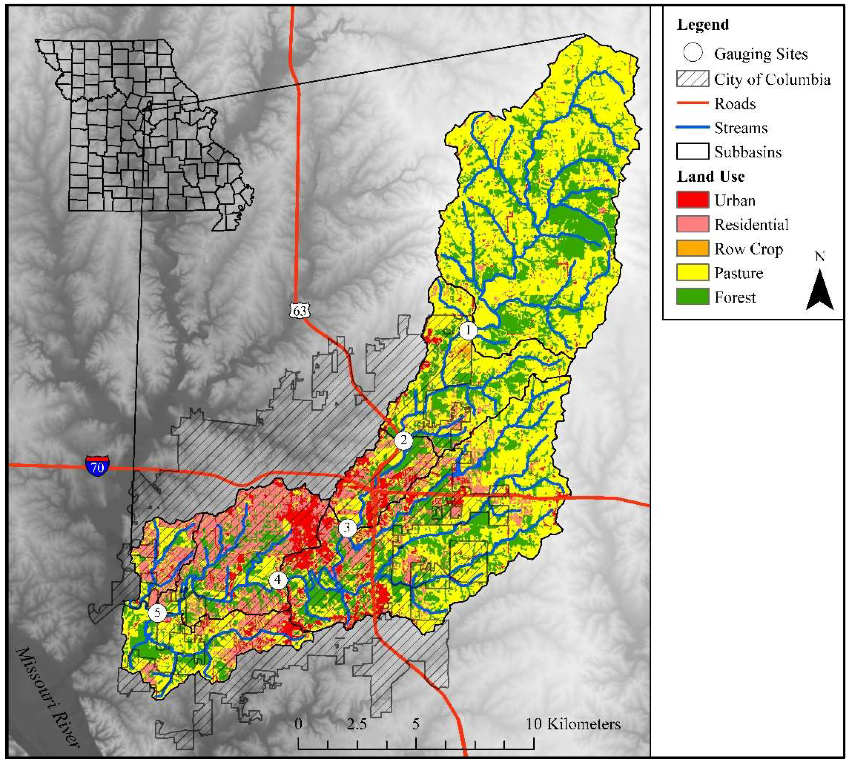
Hinkson Creek Watershed (HCW) is a mixed-land-use (i.e., 32% forested, 39% agricultural, 26% urban, and 3% wetland/water) catchment, which was located in the Lower Missouri River Basin (Figure 1). The catchment has a drainage area of approximately 228 km2 and elevations that range from 274 m above mean sea level (AMSL) in the headwaters to 177 m AMSL at the outlet. The headwaters of HCW are primarily rural agricultural lands and forested areas; and, the lower reaches are mostly urbanized (Table 1). Approximately 60% of the city of Columbia, Missouri (population 113,225) is located in the lower elevations [35].
Soils in HCW are comprised of poorly drained to well drained prairie-forest transitional soils [36]. Mexico-Leonard series soils in the headwaters are clay loam till soils that were underlain by Pennsylvanian sandstone. Weller-Bardley-Clinkenbeard series soils in the lower reaches are composed of cherty clay solution residuum underlain by Mississippian limestone [36,37]. Soils in the headwaters are associated with increased surface runoff potential (hydrologic groups C and D) with infiltration rates that were as low as 0.001 cm h−1 [38] due to the presence of a well-developed claypan of smectitic minerals found in the argillic (Bt) horizon. Floodplain alluvial soils in the lower reaches have infiltration rates ranging from 0.1 cm h−1 at agricultural sites to 126.0 cm h−1 at bottomland hardwood forest sites [39].
Climate in Missouri is dominated by maritime and continental tropical air masses in the summer and continental polar air masses in the winter (http://climate.missouri.edu/). A recent 18-year climate record (2000–2017) showed average air temperature and annual total precipitation of 13.5 °C and 967 mm, respectively, in HCW. Air temperatures ranged from −23.1 °C to 41.3 °C. A well-defined wet season occurs during spring (April to June), and a relatively sporadic wet season occurs during early fall (September to October) [40].
The main channel of HCW, Hinkson Creek, is approximately 56 km in length (including meandering) (Table 1); flowing southwesterly from the headwaters in Hallsville, Missouri through Columbia, Missouri to its confluence with Perche Creek. After confluence with Perche Creek, Hinkson Creek flows approximately 18 km (including meandering) through Perche Creek to its confluence with Missouri River. During winter 2008, Hinkson Creek was instrumented with a nested-scale experimental watershed study design [41]. Five hydroclimate gauging sites were positioned along the main channel to divide HCW into five sub-basins. (Table 1, Figure 1). Site #5 is located near the watershed outlet, and Sites #1 to #4 are nested within (Figure 1). At Site #4, the stage of Hinkson Creek has been intermittently monitored since 1967 using a USGS gauging station (#06910230).
2.2. Data Collection
Precipitation and stage were monitored at each site (n = 5) during the study period (2010–2014) (Figure 1). Rainfall was sensed using TE525WS tipping bucket rain gauges with an accuracy of +1% at 2.5 cm h−1 rainfall rate to −3.5% at 5.1 to 7.6 cm h−1 rainfall rate. Stage was sensed using Sutron Accubar® constant flow bubblers with accuracy of 0.02% at 0–7.6 m to 0.05% at 7.6–15.4 m. Precipitation and stage data were stored on Campbell Scientific CR-1000 data loggers. Methods that were used to estimate discharge included standards that were published by Turnipseed and Saur (2010) [42]. Stream velocity was measured using FLO-MATE™ Marsh McBirney flow meters and wading rods when stage was less than 1-m deep. Storm flows were measured using a USGS Bridge Board™. Stage-discharge rating curves were generated using the incremental cross section method to estimate stream flow [43].
2.3. Pre-Development SWAT Modeling
The SWAT model was used to simulate hydrologic conditions of a loading regime during pre-development conditions (circa 1800) at each gauging site in HCW. The model was previously calibrated and validated at each gauging site concurrently from the headwaters to the watershed outlet using four years of observed daily streamflow, sediment, phosphorus, and nitrogen data in the study catchment [44]. The process included auto-calibration using SWAT-cup as per methods that were published by Arnold et al., 2012 [34]. Calibration parameters were carefully adjusted during auto-calibration to keep the parameters within physically realistic bounds [34,44]. This and additional information regarding the input datasets and model forcing’s can be found in Zeiger and Hubbart (2016) [44].
Land use and land cover was converted from a calibrated SWAT model [44], as per recommendations that were published by Bressiani et al., 2015, who suggested using a calibrated SWAT model prior to land cover conversion to simulate pre-European development land use and stream management conditions [45]. The effects of land use and land cover changes on loading regimes were the focus of this research, therefore, current climate and elevation input data were used as inputs in the SWAT model [45]. National Land Cover Dataset (NLCD 2011) input data were converted to native land cover dependent on soil characteristics using NRCS-USDA ESD and OSD. For example, all the areas with ‘Mexico’ soils were assumed native grassland land cover pre-development, and areas with ‘Weller’ soils were assumed forested land cover pre-development. Management operations were changed to reflect native vegetation. For example, native grassland land cover was attributed ‘tall fescue’ and forested land cover was attributed deciduous tree cover. Soil Conservation Service curve numbers (CN2; a parameter that controls surface runoff) and overland roughness (OV_N; a parameter that controls surface roughness) parameters were updated to reflect native land cover under ‘good’ conditions using values that were provided in the USDA Technical Release 55 [46]. Urban Harvester soils where converted to native soils that are located in the sub-basin (e.g., Weller soils) to simulate pre-development conditions as Harvester soils are described in an USDA OSD as “disturbed materials in areas where loess deposits that have been graded and reshaped for urban and suburban development”. All of the other model parameters were left at default excepting parameters adjusted during model calibration outlined in Zeiger and Hubbart (2016) [44]. In summary, the general work flow of pre-development SWAT modeling was completed in the following six steps: (1) SWAT was set-up using contemporary elevation, soils, land use and land cover (LULC), climate and management operations data in HCW [44], (2) SWAT was calibrated and validated at each sub-basin concurrently from the headwaters to the watershed outlet using four years of observed stream flow, sediment, nitrogen, and phosphorus data collected at five nested gauging sites in HCW [44], (3) LULC was updated to reflect native land cover prior to European settlement (circa 1800), the SWAT parameter database (SWAT2012.mdb) was updated to reflect native land cover prior to European settlement (circa 1800), (4) SWAT input files were re-written, (5) SWAT was run, and (6) model output data were exported for comparison of simulated pre-development conditions and observed developed conditions.
2.4. Statistical Analysis
A USGS R package EflowStats was downloaded (https://github.com/USGS-R/EflowStats) and was used to calculate 171 ‘ecologically relevant’ hydrological indices [11] at each gauging site in HCW. A detailed description of the 171 indices that were included in EflowStats can be found in “Users’ Manual for the Hydroecological Integrity Assessment Process Software” [33]. Ultimately, 171 hydrological indices were calculated from four-year daily sediment and nutrient loading records during baseline conditions (i.e., SWAT simulated pre-development sediment and nutrient loading regimes) and observed current developed conditions at each gauging site. Principal components analysis was performed to examine intercorrelation and to minimize multicollinearity among indices [11,13]. One primary index was selected for each major element of a loading regime, including magnitude, frequency, duration, timing, and rate of change across low, average and high flows, similar to methods used by Olden and Poff (2003) to define a natural flow regime [13]. A total of eight flow elements were considered in this study, including low, average, and high magnitude; low and high duration, frequency, timing, and rate of change. Olden and Poff (2003) divided flow magnitude indices (n = 94) into average, high, and low flow sub-categories, while flow duration (n = 44) and flow frequency indices (n = 14) were divided into high and low flow sub-categories. Timing (n = 10) and rate of change indices (n = 9) were not divided into sub-categories for a grand total of nine sub-categories. In the current work, the sub-categories were considered excepting low frequency (n = 3) and high flow frequency indices (n = 11) were lumped into one category that was termed ‘frequency’, similar to how Olden and Poff (2003) lumped average (n = 3), high (n = 4), and low flow (n = 3) timing variables into one category termed ‘timing’.
The PCA analyses were conducted using an R software package FactoMineR that was published by Lê, Sébastien et al., 2008 [47]. Broken-stick models were used to select the number of statistically significant principal components where the number of observed eigenvalues that exceeded simulated random eigenvalues showed the appropriate number of principal component axes for use in final PCA [48]. Results from PCA, in part, showed extracted eigenvectors (i.e., loadings) to each hydrologic index for each principal component axis. Absolute ‘loadings’ were sorted in ascending order to isolate indices that explained the most variance along each principal component axes [11,13]. Indices were ranked by loadings. Ranks were summed across all loading regimes (i.e., sediment, TIN, and TP) to select a subset of eight indices by greatest overall rank. The subset of eight indices was used to calculate loading targets corresponding to each key component of a loading regime at each gauging site.
3. Results
3.1. Pre-Development SWAT Modeling
Climate inputs included wet (precipitation = 1323 mm), average (precipitation = 984 mm), and dry years (precipitation = 668 mm), in compliance with model calibration guidelines that were suggested by Arnold et al., 2012 [34], who suggested that the model calibration period should include wet, average, and dry years (Table 2). Air temperatures ranged from −28.7 °C during winter months to 42.8 °C during summer months with an annual mean air temperature of 14.1 °C, and total solar ranged from 0.5 to 29.5 MJ m−2, with a mean of 13.5 MJ m−2 (Table 2). When considering that current climate and topography inputs were used in pre-development SWAT model simulations, observed differences in discharge and loading regimes were assumed due to land use and land cover changes.
Differences in mean daily discharge between observed developed and simulated pre-development ranged from −0.6 m3 s−1 (rural Site #2) to 0.5 m3 s−1 (urban Site #5), showing that discharge generally decreased at rural sites and increased at urban sites following land use and land cover changes (Table 3). Similarly, average annual total discharge generally decreased in the rural headwaters and increased in the lower urbanizing reaches. Differences in median daily discharge between observed developed and simulated pre-development ranged from −0.4 m3 s−1 (rural Site #1) to −0.7 m3 s−1 (urban Site #4), indicating decreased median discharge following development at each gauging site. Differences in maximum daily discharge between observed developed and simulated pre-development ranged from 12.1 m3 s−1 (rural Site #1) to 166.0 m3 s−1 (urban Site #5) showing increased maximum daily discharge at each gauging site. Variability in daily discharge increased by 0.9 m3 s−1 (rural Site #2) to 6.9 m3 s−1 (urban Site #5). These results from SWAT simulations correlated land use and land cover alterations to the magnitude of discharge in HCW. These results indicated that land use and land cover alterations have increased surface runoff and the subsequent streamflow response at rural and urban sites of the study catchment. While median discharge decreased at rural sites, maximum discharge and human impacts on sediment and nutrient inputs increased sediment and nutrient yields in HCW. However, identifying the specific hydrologic mechanisms that decreased base flow at rural sites and increased the base flow at urban sites was beyond the scope of the current work. Mean daily sediment, TIN, and TP loading generally increased by an order of magnitude as average annual total loading increased from one to three orders of magnitude following the development in HCW. For example, observed developed mean daily sediment loads ranged from 13.2 to 68.1 Mg day−1, while simulated pre-development mean daily sediment loads ranged from 0.2 to 13.4 Mg day−1. Observed developed average annual total sediment loads ranged from 4812.2 to 24,877.2 Mg day−1, while simulated pre-development average annual total sediment loads ranged from 62.1 to 4907.9 Mg day−1. Results showed that, on average, annual total nutrient loads increased from 842 to 25,823 kg day−1 (TIN), and 322 to 5045 kg day−1 (TP). Thus, while simulated average annual total discharge decreased in the headwaters, the results showed consistent increases in sediment and nutrient export due to land use and land cover changes in HCW.
3.2. Statistical Analysis
Broken-stick models indicated the number of statistically significant principal component axes to consider ranged from 1 to 4 (PC1–PC4) (Table 4, Figure 2). The principal component axes were orthogonal, and thus, independent. The first principal component (PC1) spanned the direction of the most variation in loading indices, the second principal component (PC2) spanned the direction of the second most variation in loading indices, and so on. Results showed PC1 explained 38 to 81% of the variation in loading indices with eigenvalues that ranged from 4.2 to 28.3. The second principal component explained an additional 7 to 35% of the cumulative variance in loading indices with eigenvalues that ranged from 1.1 to 13.9. There was no clear difference of intercorrelation between sediment, TIN and TP loading indices.
3.3. Loading Targets
Results from PCA indicated that a total of 20 unique loading statistics explained the most variance among 171 loading indices of PC1 across all of the loading regimes (i.e., sediment, TIN, and TP) in the study catchment. Ranking indices by “loadings” of PC1 across all of the loading regimes reduced the 171 loading indices to a subset of eight indices appropriate for loading targets in the study catchment. The subset of indices with greatest rank included: (1) median load during January (ma12), (2) median maximum load during January (ml1), (3) the average load for events above seven times the median (mh23), (4) annual minimum of 90-day moving average load (dl15), (5) annual maximum of one-day moving average daily load (dh1), (6) average number of events with loads above the 75th percentile (fh1), (7) loading constancy (ta1), and (8) variability in rise rate (ra2).
Average and low magnitude loading indices (ma12 and ml1) were generally greater during observed developed conditions with the largest differences in TIN loading. For example, observed ma12 (TIN) ranged from 3.4 to 16.9 kg day−1, while the simulated pre-development ma12 (TIN) ranged from 0.5 to 1.8 kg day−1 (Table 6). Average daily maximum load (dh1) was consistently greater during the observed developed conditions, especially for sediment loading. Observed dh1 (sediment) ranged from 1320 to 6930 Mg day−1, and simulated dh1 (sediment) ranged from 11 to 477 Mg day−1. Loading frequency was generally lesser at urban sites (Sites #3, #4, and #5) during developed conditions when compared to pre-development conditions. For example, fh1 sediment loading values were 44.5 days year−1 during pre-development conditions and 14.5 days year−1 during developed conditions at Site #3. Rate of change was consistently greater during developed conditions when compared to baseline conditions indicating increased variability in loading rise rates at all of the sites due to land use and land cover influences. For example, ra2 ranged from 437 to 736% during developed conditions and 134 to 319% during pre-development conditions. These results reflect a land use influence to loading magnitude, frequency, duration, and rate, especially during high flows.
4. Discussion
4.1. Pre-Development SWAT Modeling
The advantages and disadvantages of continuous time physically based watershed scale models, like SWAT, have been well documented [49,50,51,52], and thus, were not the focus of the current work. However, model accuracy of pre-development simulations is often unknown due to a lack of historical observed data, hence the impetus for this investigation. The methodology that is used in the current work of calibrating the SWAT model to the constituents of interest (in this case flow, sediment, nitrogen, and phosphorus) prior to land use and land cover conversion has been accepted as an appropriate method to simulate pre-European development land use and stream management conditions [45]. Thus, while it was not possible to quantify model accuracy due to a lack of historical data, calibrating the model prior to land cover conversion helped to ensure more accurate simulations of pre-development flow, sediment, and nutrient regimes.
Historical land cover reconstructions were important for understanding pre-settlement loading regimes in this research. Native land cover was estimated based on physiographic site characteristics (e.g., climate, geology, landscape position, and soils). Natural resource management agencies use such methods regularly to provide the best estimates of ecological reference site conditions that are important for management of natural resources. Native vegetation coverage of many US watersheds can be found in Ecological Site Descriptions (ESD) (https://esis.sc.egov.usda.gov/) and Official Soils Series Descriptions (OSD) (https://soilseries.sc.egov.usda.gov/) that were developed by United States Department of Agriculture National Resource Conservation Service (USDA-NRCS). Once land cover was converted and SWAT simulations were run.
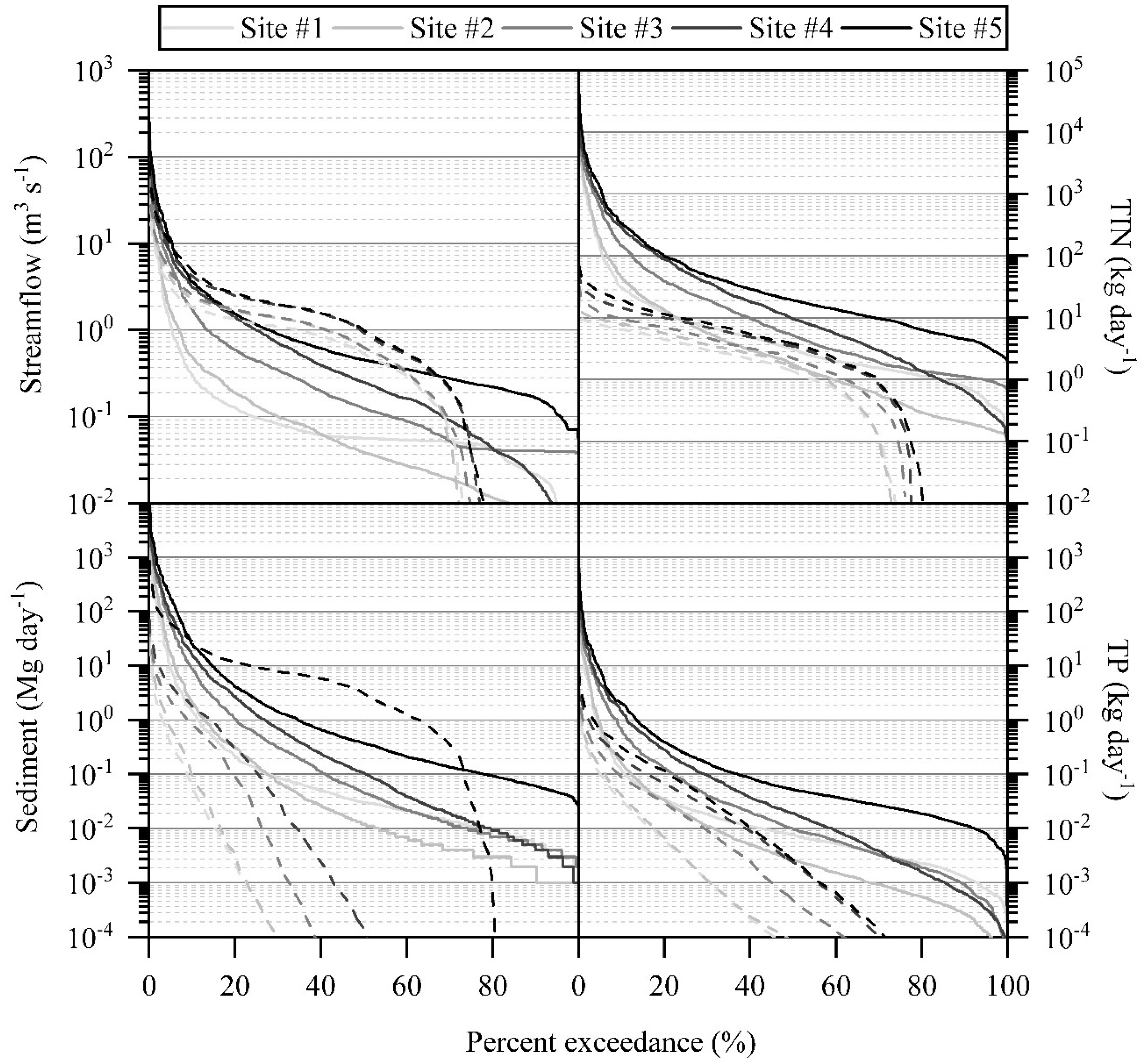
Results showed agricultural and urban development increased maximum flows, which translated to increased maximum pollutant loading in HCW. Differences in maximum streamflow ranged from 12 m3 s−1 (Site #1) to 166 m3 s−1 (Site #5). Differences in maximum daily sediment loading were relatively greater, ranging from 36 kg km−2 (Site #2) to 60 kg km−2 (Site #1). Differences in maximum daily TP loading were also large ranging from 23 kg km−2 (Site #2) to 53 kg km−2 (Site #5). Differences in maximum daily TIN loading were the greatest, ranging from 113 kg km−2 (Site #2) to 201 kg km−2 (Site #5). Increased pollutant loading was expected considering approximately 50% of total watershed area that was native forested land cover was cleared for agricultural and urban development in the study catchment. In addition, approximately 12% of the land cleared was replace with impervious surfaces associated with increased volume and velocity of surface runoff, and subsequent increases in peak flow in HCW [53]. However, the results that are indicated differences in streamflow alone did not account for the observed pollutant loading in HCW. For example, flow and load duration curves show increased median streamflow did not translate to increased median pollutant loading (Figure 2). Model simulations showed that increased pollutant export (especially TIN loading) was also due to differences in management operations (i.e., fertilizer applications, grazing, and lawn fertilizer applications).
The upper Midwest of the Missouri River Basin (MRB) has been targeted as a critical source area of sediment, N and P loading [54,55,56,57]. The greatest nitrogen fertilizer application rates of more than 2.5 t km−2 year−1 [54], with nine central states, including Missouri, which contribute more than 75% of the total N and P terrestrial loads to the Gulf of Mexico [56]. In the current work, the maximum daily loading of TIN was four orders of magnitude greater during developed conditions when compared to pre-development conditions. These results highlight substantial changes to N loading, in part, due to land use alterations to streamflow regimes, but primarily due to fertilizer applications in agricultural and urban areas of the study catchment. Thus, the restoration of pre-development stream flow regime may achieve limited results without source reductions of sediment and nutrients in HCW and similar mixed-land-use watersheds.
Results from this work are in agreement with Bernhardt et al., 2008 and others [58,59,60], in that a small fraction of N was exported during pre-development conditions while excessive nutrient enrichment was observed during developed conditions. Major anthropic sources of N included crop and lawn fertilization, soybean cultivation, and grazing. Ultimately, results from the current work in combination with other regional studies show anthropogenic sources of increased N production have substantially altered N loading regimes [58,61].
4.2. Statistical Analysis
Similar assumptions and limitations that are associated with environmental flows assessment using PCA were also applicable to the current work. For example, indices dependent on drainage area were area-normalized for better site comparison [11], which reduced variability that is important in the selection of loading targets using PCA. Additionally, PCA results are a product of statistical tests that are not physically-based. Selecting loading indices based on statistical results can be problematic when selected targets are not casually linked to loading alteration. Therefore, results should be carefully examined and validated against process-based understanding to ensure that indices are physically meaningful.
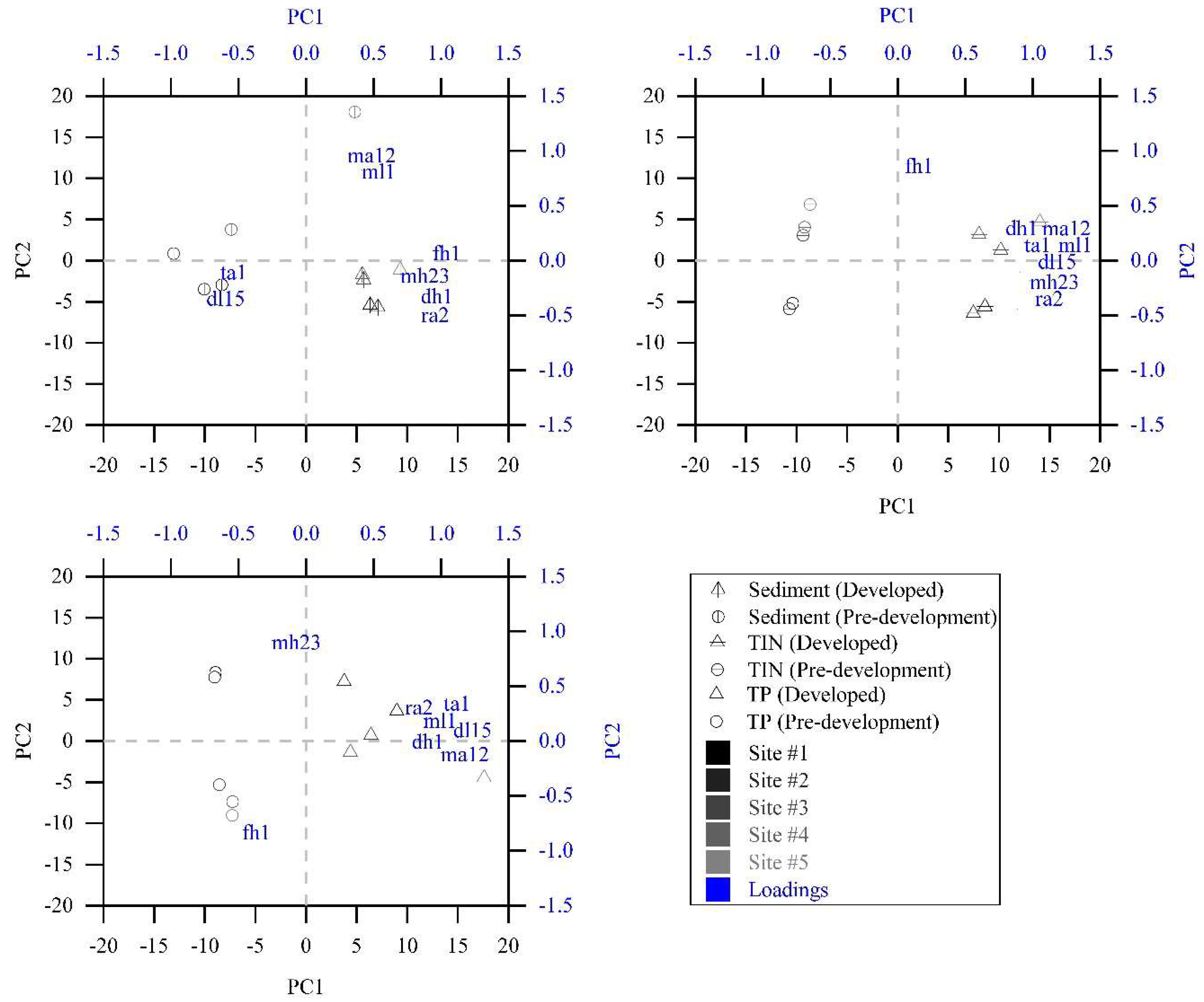
When the deviation between simulated pre-development and observed developed loading indices were examined using bi-plots, and the results showed a clear separation of pre-development and developed loading indices along the first principle component axes (PC1) (Figure 3). The second principal component axes (PC2) generally represented the effects of spatial scale on indices between sites as the drainage area increased from Site #1 in the headwaters to Site #5 near the watershed outlet (Figure 3). The loading indices that were ranked by absolute loading values for each major element of the loading regime and the results are also shown in bi-plots (Figure 3). Indices with the greatest absolute distance from the origin in the bi-plot explained the most variability in the group of 171 indices. Land use and land cover conversion (associated with PC1) had greater influence on the loading regime than the effects of scale (associated with PC2) in the study catchment with the exception of pre-development sediment simulations where sediment loads increased between Sites #4 and #5 (Figure 3).
4.3. Loading Targets
Flow, sediment, and nutrient loading regimes shape aquatic communities [10,14,58], as long-term patterns of water, sediment, and nutrient availability facilitate the spatial arrangement of soils, microclimate, and hillslope hydraulic flow paths [58]. In the current work, pre-development conditions were associated with increased retention and decreased export of flow, sediment, and nutrients when compared to developed watersheds. These results, in combination with previous literature [58], highlight potential ecological implications of land use induced loading alteration observed in Hinkson Creek and point to the need for loading targets to support ecological health.
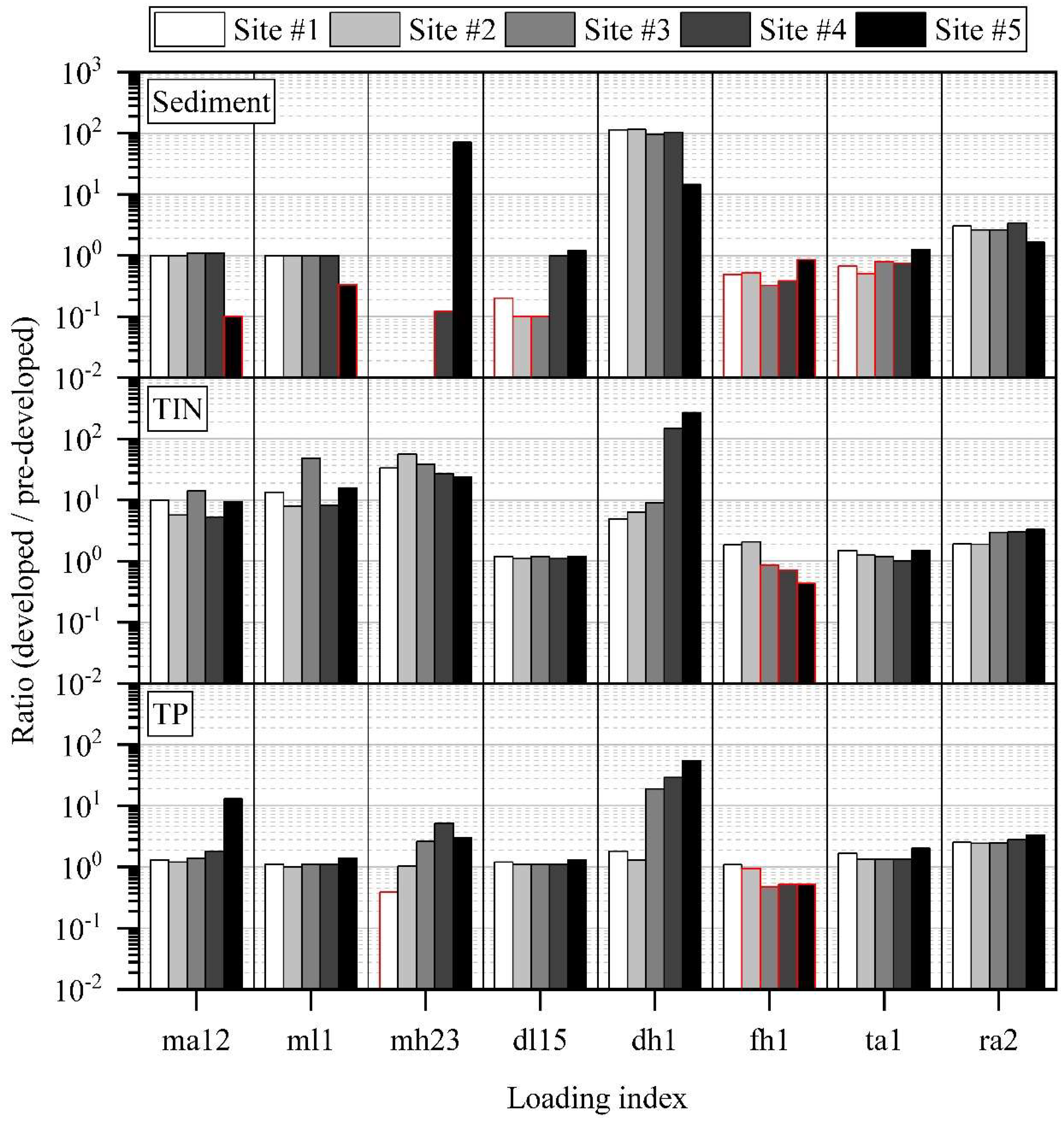
Results showed land use induced loading alterations were evident across every major element of the sediment and nutrient loading regimes in the study catchment, especially high load magnitude and duration (Figure 4). For example, annual maximum of one-day moving average daily load (dh1) was associated with differences between pre-development and developed conditions that ranged from 1307 to 6452 Mg day−1 (sediment), 5 to 27 kg day−1 (TIN), and 1 to 5 kg day−1 (TP). Results indicated the increase in dh1 was attributed to (1): land use and land cover alterations to the volume and velocity of surface runoff, and (2) management operations (e.g., tillage, lawn and crop fertilization, grazing, and soybean cultivation) that increased the export of sediment and nutrients. Previous research in the study catchment showed nearly all suspended sediment and nutrient loads were exported during high flow interval (e.g., 99% of suspended sediments, 92% of TIN, and 95% of TP loads) [40]. Results from the current work show that development has increased maximum annual daily load of sediment and nutrient export by 3 to 4 orders of magnitude in HCW.
Previous studies have reported land use alterations to the frequency of flow and non-point source pollutant delivery to receiving waters, especially in urban areas [62,63]. However, high load frequency (fh1) showed reductions to fh1 at urban Sites #3, #4, and #5 near the watershed outlet. The index fh1 was defined as the average number of events with loads that were above a threshold equal to the 75th percentile. Differences in fh1 were attributed to differences in the 75th percentile of loading between pre-development and developed conditions. For example, the 75th percentile of sediment loading threshold was 18.7 kg day−1 during pre-development conditions when compared to 566.6 kg day−1 during developed conditions at Site #3. These results indicated that management efforts focused on restoring a pre-development sediment regime should increase fh1 of sediment delivery at Site #3. However, it is important to note that increasing fh1 would only be appropriate coupled to a 30% reduction to the 75th percentile of sediment loading. Additional research is needed to validate the efficacy of loading targets based on a pre-development loading regime in contemporary mixed-land-use watersheds that have been extensively altered by past and present land uses.
Restoration of a natural loading regime may not be practical in developed watersheds. There are best management practices (BMPs) that can increase the residence time and the retention of pollutant loads by diverting runoff to naturally occurring near-surface valley bottom storage (e.g., bottomlands, wetlands, bank soils, and alluvial fills) [62,64]. However, the megatons of N and P fertilizers applied during March in the Mississippi River Basin is not a natural magnitude and timing of nutrient inputs for undeveloped watersheds. Such nutrient enrichment has caused extensive and wide-spread impairment to receiving waters [54,56,57]. Thus, source contributions will also need to be managed effectively to achieve loading targets that are based on pre-development loading regimes, especially nutrients in the study catchment.
4.4. Study Implications and Future Work
The progression of management efforts from sustaining minimum flows and the reduction of point source pollutant loading, to the restoration of a natural flow regime and the reduction of non-point source pollutant loading has helped to improve water quality and ecological health in the US. A focus on reductions to point and non-point source loading have been justified while considering that the magnitude of total loading is usually the most altered aspect of loading regimes currently. However, alterations to the duration, frequency, timing, and rate of change in loading have also been reported [14,62]. Building on work from Poff et al., 1997, Wohl et al., 2015 discussed how flow management plans that do not consider sediment inputs might achieve limited success considering aquatic ecosystem health depends on adequate flow and sediment regimes [10,14]. Results from this research are in agreement with Wohl et al., 2015 [14], there is a need to broaden the environmental flow assessment and load reduction efforts to account for alterations to all major aspects of loading regimes.
Building on work from Wohl et al., 2015 [14], the results from this study show that nutrient regimes can be more extensively altered than flow and sediment regimes in the central US. About 7% of assessed stream miles have been deemed threatened or impaired with flow alteration, while over 20% of assessed miles are threatened or impaired with sediment and/or nutrient alterations in the US. [5], with extensive nutrient alterations being reported in the Mississippi River Basin [54,56,57]. Such wide-spread impairment drives the impetus for future work that is focused on development of regional flow and loading targets to restore pre-development flow and loading remiges. Results from this assessment show the same methodologies outlined in regional environmental flows assessment frameworks (e.g., ELOHA and HIP) could be expanded to include loading targets as being appropriate for a more holistic approach to regional stream and river management.
5. Conclusions
Human land use, land-change related impacts have caused wide-spread alterations to flow and pollutant loading regimes, and the current pace of impairment exceeds mitigation efforts globally. The current work assessed the efficacy of loading targets based on SWAT simulated pre-development loading regimes in a contemporary mixed-land-use catchment. This modeling application was possible due to the long-term monitoring of precipitation, stage, and water quality constituents at nested gauging sites in the study catchment.
Results showed land use impacts to each major element of sediment and nutrient loading regimes in HCW. Differences in maximum daily loading were 55 Mg km−2 (sediment), 201 kg km−2 (TIN), and 53 kg km−2 (TP) at urban Site #5 near the watershed outlet. Land use alterations to high load duration (dh1) were also apparent with differences that ranged from 1307 to 6452 Mg day−1 (sediment), 5 to 27 kg day−1 (TIN), and 1 to 5 kg day−1 (TP) between pre-development and developed conditions. Variability in the rise rate of loading was two to three times greater during developed conditions. These results indicated that loading targets dependent on pre-development loading regimes may not be socioeconomically practical in watersheds already extensively altered by land use. Ultimately, there is a need for practical loading targets that support balanced flow, sediment, and nutrient regimes to guide regional stream and river management.
Author Contributions
Data curation, S.J.Z.; Formal analysis, S.J.Z.; Funding acquisition, J.A.H.; Project administration, J.A.H.; Writing—original draft, S.J.Z.; Writing—review & editing, J.A.H.
Funding
This research was funded by the Missouri Department of Conservation and the U.S. Environmental Protection Agency Region 7 through the Missouri Department of Natural Resources (P.N: G08-NPS-17) under Section 319 of the Clean Water Act and through joint agreement of the University of Missouri, the City of Columbia, and Boone County Public works and partners of the Hinkson Creek Collaborative Adaptive Management (CAM) program. Additional funding was provided by the National Science Foundation under Award Number OIA-1458952, the USDA National Institute of Food and Agriculture, Hatch project accession number 1011536, and the West Virginia Agricultural and Forestry Experiment Station. Results presented may not reflect the views of the sponsors and no official endorsement should be inferred.
Acknowledgments
Special thanks are due to many scientists of the Interdisciplinary Hydrology Laboratory (www.forh2o.net).
Conflicts of Interest
The authors declare no conflict of interest.
References
- Turner, R.E.; Rabalais, N.N. Suspended sediment, C, N, P and Si yields from the Mississippi River Basin. Hydrobiologia 2004, 511, 79–89. [Google Scholar] [CrossRef]
- Roy, A.H.; Freeman, M.C.; Freeman, B.J.; Wenger, S.J.; Ensign, W.E.; Meyer, J.L. Investigating hydrological alteration as a mechanism of fish assemblage shifts in urbanizing streams. J. N. Am. Benthol. Soc. 2005, 24, 656–678. [Google Scholar] [CrossRef]
- David, M.B.; Gentry, L.E. Anthropogenic inputs of nitrogen and phosphorus and riverine export for Illinois, USA. J. Environ. Q. 2000, 29, 494–508. [Google Scholar] [CrossRef]
- Poff, N.L.; Richter, B.D.; Arthington, A.H.; Bunn, S.E.; Naiman, R.J.; Kendy, E.; Henriksen, J. The ecological limits of hydrologic alteration (ELOHA): A new framework for developing regional environmental flow standards. Freshw. Biol. 2010, 55, 147–170. [Google Scholar] [CrossRef]
- Environmental Protection Agency (EPA). Water Quality Assessment and TMDL Information. Available online: https://ofmpub.epa.gov/waters10/attains_index.home (accessed on 16 March 2018).
- Dodds, W.K.; Bouska, W.W.; Eitzmann, J.L.; Pilger, T.J.; Pits, K.L.; Riley, A.J.; Schloesser, J.T.; Thornbrugh, D.J. Eutrophication of USA freshwaters: Analysis of potential economic damages. Environ. Sci. Technol. 2009, 43, 12–19. [Google Scholar] [CrossRef] [PubMed]
- Bilotta, G.S.; Brazier, R.E. Understanding the influence of suspended solids on water quality and aquatic biota. Water Res. 2008, 42, 2849–2861. [Google Scholar] [CrossRef] [PubMed]
- Jacobson, C.R. Identification and quantification of the hydrological impacts of imperviousness in urban catchments: A review. J. Environ. Manag. 2011, 92, 1438–1448. [Google Scholar] [CrossRef] [PubMed]
- Cohen, J.E. Human population: The next half century. Science 2003, 302, 1172–1175. [Google Scholar] [CrossRef] [PubMed]
- Poff, N.L.; Allan, J.D.; Bain, M.B.; Karr, J.R.; Prestegaard, K.L.; Richter, B.D.; Stromberg, J.C. The natural flow regime. Bioscience 1997, 47, 769–784. [Google Scholar] [CrossRef]
- Kennen, J.G.; Henriksen, J.A.; Heasley, J.; Cade, B.S.; Terrell, J.W. Application of the hydroecological integrity assessment process for Missouri streams. USA Geol. Sur. Sci. Investig. Rep. 2009, 1138, 57. [Google Scholar]
- Acreman, M.C.; Dunbar, M.J. Defining environmental river flow requirements? A review. Hydrol. Earth Syst. Sci. Dis. 2004, 8, 861–876. [Google Scholar] [CrossRef]
- Olden, J.D.; Poff, N.L. Redundancy and the choice of hydrologic indices for characterizing streamflow regimes. River Res. Appl. 2003, 19, 101–121. [Google Scholar] [CrossRef]
- Wohl, E.; Bledsoe, B.P.; Jacobson, R.B.; Poff, N.L.; Rathburn, S.L.; Walters, D.M.; Wilcox, A.C. The natural sediment regime in rivers: Broadening the foundation for ecosystem management. Bioscience 2015, 65, 358–371. [Google Scholar] [CrossRef]
- Hughes, J.M.R.; James, B. A hydrological regionalization of streams in Victoria, Australia, with implication for stream ecology. Aus. J. Mar. Freshw. Res. 1989, 40, 303–326. [Google Scholar] [CrossRef]
- Poff, N.L.; Ward, J.V. Implications of streamflow variability and predictability for lotic community structure—A regional analysis of streamflow patterns. Can. J. Fish. Aquat. Sci. 1989, 46, 1805–1818. [Google Scholar] [CrossRef]
- Richards, R.P. Measures of flow variability for Great Lakes tributaries. Environ. Monit. Assess. 1989, 12, 361–377. [Google Scholar] [CrossRef] [PubMed]
- Richards, R.P. Measures of flow variability and a new flow-based classification of Great Lakes tributaries. J. Great Lakes Res. 1990, 16, 53–70. [Google Scholar] [CrossRef]
- Poff, N.L. A hydrogeography of unregulated streams in the United States and an examination of scale-dependence in some hydrological descriptors. Freshw. Biol. 1996, 36, 71–91. [Google Scholar] [CrossRef]
- Richter, B.D.; Baumgartner, J.V.; Braun, D.P.; Powell, J. A spatial assessment of hydrologic alteration within a river network. Regul. Rivers Res. Manag. 1998, 14, 329–340. [Google Scholar] [CrossRef]
- Richter, B.D.; Baumgartner, J.V.; Powell, J.; Braun, D.P. A method for assessing hydrologic alteration within ecosystems. Conserv. Biol. 1996, 10, 1163–1174. [Google Scholar] [CrossRef]
- Richter, B.D.; Baumgartner, J.V.; Wigington, R.; Braun, D.P. How much water does a river need? Freshw. Biol. 1997, 37, 231–249. [Google Scholar] [CrossRef]
- Clausen, B.; Biggs, B.J.F. Relation-ships between benthic biota and hydrological indices in New Zealand streams. Freshw. Biol. 1997, 38, 327–342. [Google Scholar] [CrossRef]
- Clausen, B.; Biggs, B.J.F. Flow indices for ecological studies in temperate streams: Groupings based on covariance. J. Hydrol. 2000, 237, 184–197. [Google Scholar] [CrossRef]
- Puckridge, J.T.; Sheldon, F.; Walker, K.F.; Boulton, A.J. Flow variability and the ecology of large rivers. Mar. Freshw. Res. 1998, 49, 55–72. [Google Scholar] [CrossRef]
- Clausen, B.; Iversen, H.L.; Ovesen, N.B. Ecological flow indices for Danish streams. In Nordic Hydrological Conference 2000; Nilsson, T., Ed.; Nordic Hydrological Conference: Uppsala, Sweden, 2000; pp. 3–10. [Google Scholar]
- Wood, P.J.; Agnew, M.D.; Petts, G.E. Flow variations and macroinvertebrate community responses in a small groundwater-dominated stream in south-east England. Hydrol. Proc. 2000, 14, 3133–3147. [Google Scholar] [CrossRef]
- Verstraeten, G.; Lang, A.; Houben, P. Human impact on sediment dynamics—Quantification and timing. Catena 2009, 77, 77–80. [Google Scholar] [CrossRef] [Green Version]
- Royer, T.V.; David, M.B.; Gentry, L.E. Timing of riverine export of nitrate and phosphorus from agricultural watersheds in Illinois: Implications for reducing nutrient loading to the Mississippi River. Environ. Sci. Technol. 2006, 40, 4126–4131. [Google Scholar] [CrossRef] [PubMed]
- Walsh, C.J.; Fletcher, T.D.; Burns, M.J. Urban stormwater runoff: A new class of environmental flow problem. PLoS ONE 2012, 7, e45814. [Google Scholar] [CrossRef] [PubMed]
- Zimmerman, J.K.; Vondracek, B.; Westra, J. Agricultural land use effects on sediment loading and fish assemblages in two Minnesota (USA) watersheds. Environ. Manag. 2003, 32, 93–105. [Google Scholar] [CrossRef]
- Boynton, W.R.; Kemp, W.M. Influence of river flow and nutrient loads on selected ecosystem processes and properties in Chesapeake Bay. In Estuarine Science: A Synthetic Approach to Research and Practice; Hobbie, J., Ed.; Island Press: Washington, DC, USA, 2000; pp. 269–298. [Google Scholar]
- Henriksen, J.A.; Heasley, J.; Kennen, J.G.; Nieswand, S. Users’ Manual for the Hydroecological Integrity Assessment Process Software (including the New Jersey Assessment Tools); USA Geological Survey: Reston, VA, USA, 2006.
- Arnold, J.G.; Moriasi, D.N.; Gassman, P.W.; Abbaspour, K.C.; White, M.J.; Srinivasan, R.; Santhi, C.; Harmel, R.D.; van Griensven, A.; Van Liew, M.W.; et al. SWAT: Model use, calibration, and validation. Am. Soc. Agric. Biol. Eng. 2012, 55, 1491–1508. [Google Scholar]
- United States Census Bureau (USCB). USA Census Bureau: State and County Quick Facts. 2017. Available online: http://quickfacts.census.gov/qfd/states/29000.html (accessed on 9 December 2017).
- Hubbart, J.A.; Zell, C. Considering streamflow trend analyses uncertainty in urbanizing watersheds: A baseflow case study in the central United States. Earth Interact. 2013, 17, 1–28. [Google Scholar] [CrossRef]
- Miller, D.E.; Vandike, J.E. Groundwater Resources of Missouri (Vol. 2); Missouri Department of Natural Resources, Division of Geology and Land Survey: Jefferson City, MO, USA, 1997.
- Blanco-Canqui, H.; Gantzer, C.J.; Anderson, S.H.; Alberts, E.E.; Ghidey, F. Saturated hydraulic conductivity and its impact on simulated runoff for claypan soils. Soil Sci. Soc. Am. J. 2002, 66, 1596–1602. [Google Scholar] [CrossRef]
- Hubbart, J.A.; Muzika, R.-M.; Huang, D.; Robinson, A. Improving Quantitative Understanding of Bottomland Hardwood Forest Influence on Soil Water Consumption in an Urban Floodplain. Watershed. Sci. Bull. 2011, 3, 34–43. [Google Scholar]
- Zeiger, S.J.; Hubbart, J.A. An Assessment of Mean Areal Precipitation Methods on Simulated Stream Flow: A SWAT Model Performance Assessment. Water 2017, 9, 459. [Google Scholar] [CrossRef]
- Hubbart, J.A.; Holmes, J.; Bowman, G. TMDLs: Improving stakeholder acceptance with science-based allocations. Watershed. Sci. Bull. 2010, 1, 19–24. [Google Scholar]
- Turnipseed, D.P.; Sauer, V.B. Discharge Measurements at Gaging Stations; (No. 3-A8); USA Geological Survey: Reston, VA, USA, 2010.
- Dottori, F.; Martina, M.L.V.; Todini, E. A dynamic rating curve approach to indirect discharge measurement. Hydrol. Earth Syst. Sci. 2009, 13, 847–863. [Google Scholar] [CrossRef]
- Zeiger, S.J.; Hubbart, J.A. A SWAT model validation of nested-scale contemporaneous stream flow, suspended sediment and nutrients from a multiple-land-use watershed of the central USA. Sci. Total Environ. 2016, 572, 232–243. [Google Scholar] [CrossRef] [PubMed]
- Bressiani, D.; Gassman, P.W.; Fernandes, J.G.; Garbossa, L.H.P.; Srinivasan, R.; Bonumá, N.B.; Mendiondo, E.M. Review of soil and water assessment tool (SWAT) applications in Brazil: Challenges and prospects. Int. J. Agric. Biol. Eng. 2015, 8, 9. [Google Scholar]
- United States Department of Agriculture (USDA). Urban Hydrology for Small Watersheds; US Deptartment of Agriculture, Soil Conservation Service, Engineering Division: Washington, DC, USA, 1986.
- Lê, S.; Josse, J.; Husson, F. FactoMineR: An R Package for Multivariate Analysis. J. Stat. Softw. 2008, 25, 1–18. [Google Scholar] [CrossRef]
- Jackson, D.A. Stopping rules in principal components analysis: A comparison of heuristical and statistical approaches. Ecology 1993, 74, 2204–2214. [Google Scholar] [CrossRef]
- Srinivasan, R.; Zhang, X.; Arnold, J.G. SWAT ungauged: Hydrological budget and crop yield predictions in the Upper Mississippi River basin. Trans. ASABE 2010, 53, 1533–1546. [Google Scholar] [CrossRef]
- Gassman, P.W.; Reyes, M.R.; Green, C.H.; Arnold, J.G. The Soil and Water Assessment Tool: Historical development, applications, and future research directions. Trans. Am. Soc. Agric. Biol. Eng. 2007, 50, 1211–1250. [Google Scholar] [CrossRef]
- Borah, D.K.; Yagow, G.; Saleh, A.; Barnes, P.L.; Rosenthal, W.; Krug, E.C.; Hauck, L.M. Sediment and nutrient modeling for TMDL development and implementation. Am. Soc. Agric. Biol. Eng. 2006, 49, 967–986. [Google Scholar]
- Borah, D.K.; Bera, M. Watershed-scale hydrologic and nonpoint-source pollution models: Review of mathematical bases. Trans. ASAE. 2003, 46, 1553. [Google Scholar] [CrossRef]
- Zeiger, S.J.; Hubbart, J.A. Quantifying land use influences on event-based flow frequency, timing, magnitude, and rate of change in an urbanizing watershed of the central USA. Environ. Earth Sci. 2018, 77, 107. [Google Scholar] [CrossRef]
- Mueller, D.K.; Helsel, D.R. Nutrients in the Nation’s Waters—Too much of a good thing? National Water-Quality Assessment (NAWQA) Program. Circ 1136; 2013. Available online: http://pubs.usgs.gov/circ/circ1136/ (accessed on 9 December 2017).
- Robertson, D.M.; Saad, D.A. Nutrient inputs to the Laurentian Great Lakes by source and watershed estimated using SPARROW watershed models. J. Am. Water Res. Assoc. 2011, 47, 1011–1033. [Google Scholar] [CrossRef] [PubMed]
- Alexander, R.B.; Smith, R.A.; Schwarz, G.E.; Boyer, E.W.; Nolan, J.V.; Brakebill, J.W. Differences in phosphorus and nitrogen delivery to the Gulf of Mexico from the Mississippi River Basin. Environ. Sci. Technol. 2008, 42, 822–830. [Google Scholar] [CrossRef] [PubMed]
- Howarth, R.W.; Billen, G.; Swaney, D.; Townsend, A.; Jaworski, N.; Lajtha, K.; Downing, J.A.; Elmgren, R.; Caraco, T.; Jordan, T.; et al. Regional nitrogen budgets and riverine N & P fluxes for the drainages to the North Atlantic Ocean: Natural and human influences. Biochemistry 1996, 35, 75–139. [Google Scholar]
- Bernhardt, E.S.; Band, L.E.; Walsh, C.J.; Berke, P.E. Understanding, managing, and minimizing urban impacts on surface water nitrogen loading. Ann. N. Y. Acad. Sci. 2008, 1134, 61–96. [Google Scholar] [CrossRef] [PubMed]
- Boyer, E.W.; Howarth, R.W.; Galloway, J.N.; Dentener, F.J.; Green, P.A.; Vörösmarty, C.J. Riverine nitrogen export from the continents to the coasts. Glob. Biogeochem. Cycles 2006, 20. [Google Scholar] [CrossRef]
- Green, P.A.; Vörösmarty, C.J.; Meybeck, M.; Galloway, J.N.; Peterson, B.J.; Boyer, E.W. Pre-industrial and contemporary fluxes of nitrogen through rivers: A global assessment based on typology. Biogeochemistry 2004, 68, 71–105. [Google Scholar] [CrossRef]
- Galloway, J.N.; Dentener, F.J.; Capone, D.G.; Boyer, E.W.; Howarth, R.W.; Seitzinger, S.P.; Karl, D.M. Nitrogen cycles: Past, present, and future. Biogeochemistry 2004, 70, 153–226. [Google Scholar] [CrossRef]
- Walsh, C.J.; Roy, A.H.; Feminella, J.W.; Cottingham, P.D.; Groffman, P.M.; Morgan, R.P. The urban stream syndrome: Current knowledge and the search for a cure. J. N. Am. Benthol. Soc. 2005, 24, 706–723. [Google Scholar] [CrossRef]
- Fletcher, T.D.; Mitchell, V.; Deletic, A.; Ladson, T.R.; Seven, A. Is stormwater harvesting beneficial to urban waterway environmental flows? Water Sci. Technol. 2007, 55, 265–272. [Google Scholar] [CrossRef] [PubMed]
- Burns, M.J.; Fletcher, T.D.; Duncan, H.P.; Hatt, B.E.; Ladson, A.R.; Walsh, C.J. The stormwater retention performance of rainwater tanks at the land-parcel scale. In 7th International Conference on Water Sensitive Urban Design; Barton, A.C.T.: Engineers, Australia, 2012; pp. 195–203. [Google Scholar]
Figure 1.
Nested-scale experimental watershed study design including five gauging sites located in Hinkson Creek watershed, Missouri, United States of America (USA).
Figure 1.
Nested-scale experimental watershed study design including five gauging sites located in Hinkson Creek watershed, Missouri, United States of America (USA).

Figure 2.
Simulated (dashed line) and observed (solid line) daily average flow and load duration curves at five gauging sites in Hinkson Creek, Missouri, USA. Total inorganic nitrogen is TIN, and total phosphorus is TP.
Figure 2.
Simulated (dashed line) and observed (solid line) daily average flow and load duration curves at five gauging sites in Hinkson Creek, Missouri, USA. Total inorganic nitrogen is TIN, and total phosphorus is TP.

Figure 3.
Bi-plot showing scores generated from simulated pre-development and observed developed loading data at five gauging sites in Hinkson Creek, Missouri, USA. Loadings of indices with the greatest absolute loadings for eight loading sub-components are also shown. PC1 and PC2 are principal component axes. Definitions of indices are shown in Table 5. Loading indices that overlapped were slightly offset to improve readability. Total inorganic nitrogen is TIN, and total phosphorus is TP.

Figure 4.
Ratios between observed developed and simulated pre-development loading indices at five gauging sites in Hinkson Creek, Missouri, USA. Ratios less than 1 (i.e., observed < simulated) are outlined in red. Definitions of indices are provided in Table 5. Total inorganic nitrogen is TIN, and total phosphorus is TP.


Table 1.
Cumulative drainage area, stream length, and land use and land cover area (km2) to each gauging site located in Hinkson Creek Watershed (HCW), Missouri, USA. “HCW” is cumulative of Sites #1 through #5. Cumulative percent land use and land cover (LULC) of drainage area are shown in parentheses.
| Site # | Area (km2) | Stream Length (km) | Urban (km2) | Agriculture (km2) | Forested (km2) | Wetland/Water (km2) |
|---|---|---|---|---|---|---|
| Site #1 | 77 | 20 | 3.9 (5) | 43.9 (57) | 27.7 (36) | 1.5 (2) |
| Site #2 | 101 | 27 | 6.1 (6) | 56.6 (56) | 36.4 (36) | 2.0 (2) |
| Site #3 | 114 | 32 | 12.5 (11) | 58.1 (51) | 41.0 (36) | 2.3 (2) |
| Site #4 | 180 | 40 | 28.8 (16) | 82.8 (46) | 64.8 (36) | 3.6 (2) |
| Site #5 | 206 | 49 | 47.4 (23) | 84.5 (41) | 70.0 (34) | 4.1 (2) |
| HCW | 228 | 56 | 59.2 (26) | 88.9 (39) | 73.0 (32) | 6.8 (3) |
Table 2.
Summary of daily climate statistics at a United States (US) Geological Survey gauging site (Site #4) in Hinkson Creek, Missouri, USA.
Table 2.
Summary of daily climate statistics at a United States (US) Geological Survey gauging site (Site #4) in Hinkson Creek, Missouri, USA.
| Climate Variable | Mean | St. Dev. | Min | Median | Max |
|---|---|---|---|---|---|
| Precipitation (mm) § | 984 | 240 | 668 | 973 | 1323 |
| Air temperature (°C) | 12.9 | 10.8 | −28.7 | 14.1 | 42.8 |
| Relative humidity (%) | 70.5 | 12.3 | 32.9 | 70.9 | 99.4 |
| Total solar (MJ m−2) | 13.5 | 7.5 | 0.5 | 12.9 | 29.5 |
| Wind speed (m s−1) | 1.4 | 0.8 | 0.0 | 1.3 | 5.8 |
§ Precipitation statistics were calculated from annual totals.
Table 3.
Descriptive daily statistics showing observed developed and simulated pre-development discharge, sediment, total inorganic nitrogen (TIN) and total phosphorus (TP) at five gauging sites on Hinkson Creek, Missouri, USA. Standard deviations are shown in parentheses.
Table 3.
Descriptive daily statistics showing observed developed and simulated pre-development discharge, sediment, total inorganic nitrogen (TIN) and total phosphorus (TP) at five gauging sites on Hinkson Creek, Missouri, USA. Standard deviations are shown in parentheses.
| Variable | Site # | Mean | Total § | Minimum | Median | Maximum |
|---|---|---|---|---|---|---|
| Observed | Site #1 | 0.5 (3.0) | 214.9 | <0.1 | 0.1 | 45.8 |
| Discharge | Site #2 | 0.7 (3.6) | 207.9 | <0.1 | <0.1 | 61.0 |
| (m3 s−1) | Site #3 | 1.3 (5.0) | 344.8 | <0.1 | 0.1 | 70.0 |
| Site #4 | 2.0 (8.2) | 354.3 | <0.1 | 0.2 | 141.2 | |
| Site #5 | 2.9 (12.7) | 444.1 | 0.1 | 0.5 | 251.6 | |
| Simulated | Site #1 | 1.0 (2.0) | 396.6 | <0.1 | 0.5 | 33.7 |
| Discharge | Site #2 | 1.3 (2.7) | 386.2 | <0.1 | 0.6 | 46.6 |
| (m3 s−1) | Site #3 | 1.4 (3.2) | 375.6 | <0.1 | 0.6 | 54.7 |
| Site #4 | 2.2 (5.0) | 375.5 | <0.1 | 0.9 | 79.6 | |
| Site #5 | 2.4 (5.8) | 370.0 | <0.1 | 1.0 | 85.6 | |
| Observed | Site #1 | 13.2 (147.9) | 4812.2 | <0.1 | <0.1 | 4617.5 |
| Sediment | Site #2 | 20.1 (179.7) | 7349.0 | <0.1 | <0.1 | 3657.2 |
| (Mg day−1) | Site #3 | 30.8 (239.3) | 11,234.5 | <0.1 | <0.1 | 5789.2 |
| Site #4 | 43.0 (356.1) | 15,688.9 | <0.1 | 0.1 | 8317.5 | |
| Site #5 | 68.1 (529.3) | 24,877.2 | <0.1 | 0.4 | 12,103.5 | |
| Simulated | Site #1 | 0.2 (1.2) | 62.1 | <0.1 | <0.1 | 26.4 |
| Sediment | Site #2 | 0.3 (2.2) | 112.7 | <0.1 | <0.1 | 48.3 |
| (Mg day−1) | Site #3 | 0.6 (3.0) | 208.2 | <0.1 | <0.1 | 59.0 |
| Site #4 | 0.9 (4.2) | 342.5 | <0.1 | <0.1 | 69.7 | |
| Site #5 | 13.4 (44.9) | 4907.9 | <0.1 | 3.1 | 851.1 | |
| Observed | Site #1 | 70.7 (494.2) | 25,833.4 | 0.1 | 3.1 | 10,463.4 |
| TIN | Site #2 | 82.7 (543.1) | 30,188.4 | 0.1 | 1.7 | 11,460.0 |
| (kg day−1) | Site #3 | 152.5 (811.5) | 55,698.3 | 0.6 | 5.2 | 15,093.0 |
| Site #4 | 237.0 (1327) | 86,557.9 | 0.1 | 9.6 | 25,155.8 | |
| Site #5 | 356.7 (2136.7) | 130,285.6 | 1.8 | 19.1 | 41,435.0 | |
| Simulated | Site #1 | 2.3 (2.7) | 842.4 | <0.1 | 1.4 | 24.3 |
| TIN | Site #2 | 2.8 (3.4) | 1031.7 | <0.1 | 1.6 | 30.3 |
| (kg day−1) | Site #3 | 3.7 (4.5) | 1344.0 | <0.1 | 2.2 | 34.9 |
| Site #4 | 5.6 (6.9) | 2042.2 | <0.1 | 3.5 | 56.5 | |
| Site #5 | 7.0 (9.4) | 2549.0 | <0.1 | 3.8 | 71.0 | |
| Observed | Site #1 | 13.8 (107.7) | 5045.3 | <0.1 | 0.4 | 2582.6 |
| TP | Site #2 | 15.3 (111.5) | 5574.7 | <0.1 | 0.2 | 2451.4 |
| (kg day−1) | Site #3 | 28.2 (174.7) | 10,292.4 | <0.1 | 0.6 | 4006.2 |
| Site #4 | 42.0 (266.5) | 15,356.3 | <0.1 | 1.0 | 6245.7 | |
| Site #5 | 65.9 (447.9) | 24,064.2 | <0.1 | 2.4 | 11,010.9 | |
| Simulated | Site #1 | 0.9 (3.8) | 322.3 | <0.1 | <0.1 | 70.2 |
| TP | Site #2 | 1.1 (5.1) | 415.0 | <0.1 | <0.1 | 96.7 |
| (kg day−1) | Site #3 | 1.9 (6.9) | 682.4 | <0.1 | <0.1 | 124.4 |
| Site #4 | 3.3 (10.8) | 1220.0 | <0.1 | 0.2 | 179.0 | |
| Site #5 | 4.6 (13.6) | 1667.6 | <0.1 | 0.2 | 202.8 |
§ Total shows average annual total discharge (mm), sediment (Mg year−1), TIN (kg year−1) and TP (kg year−1).
Table 4.
Indices with greatest absolute loadings of each principal component axis (PC1–PC4) represent each major element of a loading regime in Hinkson Creek, Missouri, USA. Average is ‘ave’. Definitions of indices are located in Table 5. Total inorganic nitrogen is TIN, and total phosphorus is TP.
Table 4.
Indices with greatest absolute loadings of each principal component axis (PC1–PC4) represent each major element of a loading regime in Hinkson Creek, Missouri, USA. Average is ‘ave’. Definitions of indices are located in Table 5. Total inorganic nitrogen is TIN, and total phosphorus is TP.
| Variable | Loading Element | PC1 | PC2 | PC3 | PC4 |
|---|---|---|---|---|---|
| Sediment | Magnitude (ave) | ma16 (0.236) | ma9 (0.236) | ma45 (0.339) | ma21 (0.337) |
| Magnitude (low) | ml1 (0.295) | ml19 (0.363) | ml13 (0.545) | ||
| Magnitude (high) | mh26 (0.248) | mh10 (0.391) | mh3 (0.352) | ||
| Duration (low) | dl12 (0.363) | dl2 (0.424) | dl5 (0.462) | ||
| Duration (high) | dh20 (0.272) | dh9 (0.368) | dh6 (0.398) | ||
| Frequency | fh1 (0.307) | ||||
| Timing | ta1 (0.412) | th2 (0.516) | ta3 (0.614) | ||
| Rate of Change | ra5 (0.119) | ra3 (0.188) | |||
| TIN | Magnitude (ave) | ma9 (0.187) | ma17 (0.285) | ma34 (0.452) | |
| Magnitude (low) | ml1 (0.249) | ml5 (0.469) | |||
| Magnitude (high) | mh5 (0.230) | mh10 (0.307) | |||
| Duration (low) | dl6 (0.296) | dl7 (0.539) | |||
| Duration (high) | dh8 (0.251) | dh18 (0.384) | |||
| Frequency | fh5 (0.364) | fh4 (0.507) | |||
| Timing | ta1 (0.402) | th3 (0.580) | tl3 (0.893) | ||
| Rate of Change | ra4 (0.447) | ra6 (0.536) | |||
| TP | Magnitude (ave) | ma1 (0.191) | ma26 (0.290) | ma4 (0.269) | ma29 (0.334) |
| Magnitude (low) | ml11 (0.244) | ||||
| Magnitude (high) | mh21 (0.231) | mh13 (0.333) | mh11 (0.382) | ||
| Duration (low) | dl12 (0.313) | dl9 (0.564) | |||
| Duration (high) | dh14 (0.309) | dh12 (0.305) | dh7 (0.425) | ||
| Frequency | fh1 (0.346) | fl1 (0.581) | |||
| Timing | ta2 (0.424) | th2 (0.688) | tl1 (0.692) | ||
| Rate of Change | ra2 (0.386) | ra3 (0.718) |
Table 5.
Definitions for select indices to quantitatively define major elements of the loading regime in Hinkson Creek, Missouri, USA. Definitions were revised from Kennen et al., 2009 [11].
Table 5.
Definitions for select indices to quantitatively define major elements of the loading regime in Hinkson Creek, Missouri, USA. Definitions were revised from Kennen et al., 2009 [11].
| Index | Definition |
|---|---|
| ma1 | Average daily load of the entire study period. |
| ma4 | Standard deviation of the percentiles divided by the mean of percentiles (every 5th percentile is included). |
| ma9 | Spread in daily loading is the ratio of the difference between the 90th and 10th percentiles to median. |
| ma12-23 | Monthly median load of each month (January = ma12; December = ma23). |
| ma24-35 | Monthly coefficient of variation for each month (January = ma24; December = ma35). |
| ma45 | The mean load minus the median of the annual means divided by the median of the annual means. |
| ml1-12 | Monthly median minimum load for each month (January = ml1; December = ml12). |
| ml13 | Coefficient of variation of minimum monthly loads. |
| ml19 | The ratios of the minimum annual load to mean annual load for each year. |
| mh1-12 | Monthly median maximum load for each month (January = mh1; December = mh12). |
| mh13 | Coefficient of variation of maximum monthly loads. |
| mh21 | The average load for events above median load. |
| mh23 | The average load for events above seven times the median. |
| mh26 | The average peak load value for events above seven times the median. |
| dl2 | Annual minimum of 3-day moving average load. |
| dl5 | Annual minimum of 90-day moving average load. |
| dl6 | Variability of annual minimum daily average load. |
| dl7 | Variability of annual minimum of 3-day moving average load. |
| dl9 | Variability of annual minimum of 30-day moving average load. |
| dl12 | Annual minimum of 7-day moving average load divided by the median. |
| dh1 | Annual maximum of 1-day moving average daily load. |
| dh14 | The 95th percentile value divided by the mean of the monthly means. |
| dh18 | Average duration of events with loads above three times the median. |
| dh20 | Average duration of events with loads above the 75th percentile. |
| fl1 | Average number of events with loads below the 25th percentile. |
| fh1 | Average number of events with loads above the 75th percentile. |
| fh4 | Average days per year that the loading is above seven times the median load. |
| fh5 | Average number of loading events with loads above the median load. |
| ta1 | Loading constancy. |
| ta2 | Loading predictability. |
| ta3 | Seasonal predictability of loading. |
| th2 | Variability in Julian date of annual maxima. |
| th3 | Seasonal predictability of non-loading. |
| tl1 | Julian date of annual minimum. |
| tl3 | Seasonal predictability of low loading. |
| ra2 | Variability in rise rate. |
| ra3 | Fall rate. |
| ra4 | Variability in fall rate. |
| ra5 | Number of day rises. |
| ra6 | Median positive change of loading. |
Table 6.
Loading indices represent key elements of simulated pre-development and developed flow regimes at five gauging sites in Hinkson Creek, Missouri, USA. Definitions of indices are shown in Table 5. Total inorganic nitrogen is TIN, and total phosphorus is TP.
Table 6.
Loading indices represent key elements of simulated pre-development and developed flow regimes at five gauging sites in Hinkson Creek, Missouri, USA. Definitions of indices are shown in Table 5. Total inorganic nitrogen is TIN, and total phosphorus is TP.
| Site # | ma12 | ml1 | mh23 | dl15 | dh1 | fh1 | ta1 | ra2 | |
|---|---|---|---|---|---|---|---|---|---|
| kg day−1 | kg day−1 | -- | -- | kg day−1 | days year−1 | -- | % | ||
| Observed | Site #1 | <0.1 | <0.1 | 7461.3 | 0.2 | 1318.8 | 15.0 | 0.4 | 736.4 |
| Sediment * | Site #2 | <0.1 | <0.1 | 28,957.7 | 0.1 | 2301.3 | 15.5 | 0.3 | 635.8 |
| Site #3 | 0.1 | <0.1 | 9122.8 | 0.1 | 2531.4 | 14.5 | 0.4 | 569.5 | |
| Site #4 | 0.1 | <0.1 | 5073.4 | 0.0 | 4255.5 | 17.5 | 0.3 | 619.4 | |
| Site #5 | 0.1 | 0.1 | 2571.4 | 0.2 | 6929.6 | 17.5 | 0.5 | 522.1 | |
| Simulated | Site #1 | <0.1 | <0.1 | 1,846,953 | 1.0 | 11.6 | 30.5 | 0.6 | 242.0 |
| Sediment * | Site #2 | <0.1 | <0.1 | 3,383,306 | 1.0 | 19.9 | 29.5 | 0.6 | 241.2 |
| Site #3 | <0.1 | <0.1 | 3,698,011 | 1.0 | 26.4 | 44.5 | 0.5 | 216.5 | |
| Site #4 | <0.1 | <0.1 | 41,133.9 | 0.0 | 41.0 | 45.5 | 0.4 | 181.9 | |
| Site #5 | 1.0 | 0.3 | 36.3 | 0.0 | 477.3 | 20.5 | 0.4 | 319.3 | |
| Observed | Site #1 | 5.0 | 2.7 | 353.7 | 0.2 | 4.9 | 12.0 | 0.6 | 538.4 |
| TIN | Site #2 | 3.4 | 1.6 | 608.3 | 0.1 | 6.4 | 14.5 | 0.5 | 500.3 |
| Site #3 | 9.9 | 4.8 | 360.6 | 0.2 | 9.0 | 15.0 | 0.6 | 437.4 | |
| Site #4 | 8.5 | 4.1 | 269.4 | 0.1 | 15.0 | 15.5 | 0.5 | 444.2 | |
| Site #5 | 16.9 | 9.5 | 235.9 | 0.2 | 27.0 | 14.0 | 0.6 | 442.7 | |
| Simulated | Site #1 | 0.5 | 0.2 | 10.6 | 0.0 | <0.1 | 6.5 | 0.4 | 281.2 |
| TIN | Site #2 | 0.6 | 0.2 | 10.8 | 0.0 | <0.1 | 7.0 | 0.4 | 264.3 |
| Site #3 | 0.7 | 0.1 | 9.4 | 0.0 | <0.1 | 17.5 | 0.5 | 147.0 | |
| Site #4 | 1.6 | 0.5 | 10.0 | 0.0 | 0.1 | 21.5 | 0.5 | 145.7 | |
| Site #5 | 1.8 | 0.6 | 10.0 | 0.0 | 0.1 | 32.5 | 0.4 | 134.0 | |
| Observed | Site #1 | 0.3 | 0.1 | 444.8 | 0.2 | 0.8 | 18.0 | 0.5 | 573.0 |
| TP | Site #2 | 0.2 | <0.1 | 1100 | 0.1 | 1.3 | 15.5 | 0.4 | 548.6 |
| Site #3 | 0.4 | 0.1 | 578.9 | 0.1 | 1.9 | 17.5 | 0.4 | 499.6 | |
| Site #4 | 0.8 | 0.1 | 468.5 | 0.1 | 2.9 | 18.0 | 0.4 | 517.7 | |
| Site #5 | 1.3 | 0.4 | 349.7 | 0.3 | 5.5 | 20.0 | 0.6 | 543.3 | |
| Simulated | Site #1 | <0.1 | <0.1 | 1150.4 | 0.0 | <0.1 | 16.5 | 0.3 | 227.8 |
| TP | Site #2 | <0.1 | <0.1 | 1067.2 | 0.0 | <0.1 | 16.5 | 0.3 | 225.3 |
| Site #3 | <0.1 | <0.1 | 221.2 | 0.0 | 0.1 | 37.0 | 0.3 | 201.5 | |
| Site #4 | <0.1 | <0.1 | 90.3 | 0.0 | 0.1 | 34.5 | 0.3 | 183.2 | |
| Site #5 | 0.1 | <0.1 | 116.3 | 0.0 | 0.1 | 38.0 | 0.3 | 162.4 |
*Sediment loading indices are in Mg day-1.
© 2018 by the authors. Licensee MDPI, Basel, Switzerland. This article is an open access article distributed under the terms and conditions of the Creative Commons Attribution (CC BY) license (http://creativecommons.org/licenses/by/4.0/).
Share and Cite
MDPI and ACS Style
Zeiger, S.J.; Hubbart, J.A. Assessing the Difference between Soil and Water Assessment Tool (SWAT) Simulated Pre-Development and Observed Developed Loading Regimes. Hydrology 2018, 5, 29. https://doi.org/10.3390/hydrology5020029
AMA Style
Zeiger SJ, Hubbart JA. Assessing the Difference between Soil and Water Assessment Tool (SWAT) Simulated Pre-Development and Observed Developed Loading Regimes. Hydrology. 2018; 5(2):29. https://doi.org/10.3390/hydrology5020029
Chicago/Turabian StyleZeiger, Sean J., and Jason A. Hubbart. 2018. "Assessing the Difference between Soil and Water Assessment Tool (SWAT) Simulated Pre-Development and Observed Developed Loading Regimes" Hydrology 5, no. 2: 29. https://doi.org/10.3390/hydrology5020029
Note that from the first issue of 2016, this journal uses article numbers instead of page numbers. See further details here.