A Time Series Model Comparison for Monitoring and Forecasting Water Quality Variables

Abstract

The monitoring and prediction of water quality parameters are important tasks in the management of water resources. In this work, the performances of time series statistical models were evaluated to predict and forecast the dissolved oxygen (DO) concentration in several monitoring sites located along the main river Vouga, in Portugal, during the period from January 2002 to May 2015. The models being compared are a regression model with correlated errors and a state-space model, which can be seen as a calibration model. Both models allow the incorporation of water quality variables, such as time correlation or seasonality. Results show that, for the DO variable, the calibration model outperforms the regression model for sample modeling, that is, for a short-term forecast, while the regression model with correlated errors has a better performance for the forecasting h-steps ahead framework. So, the calibration model is more useful for water monitoring using an online or real-time procedure, while the regression model with correlated errors can be applied in order to forecast over a longer period of time.

1. Introduction

Water quality is routinely assessed in streams, rivers, lakes, and reservoirs, especially when there are significant industrial activities and human populations in these areas. Naturally, in other contexts, water quality assessment is a process that contributes to environmental and ecosystem monitoring. The analysis and monitoring of water quality through systematic and scientifically established procedures provide important information on the status of these basins, while also helping official entities target their decision-making processes toward supported policy options. For instance, in a hydrological basin, this information can be used to build an understanding of the dynamic of the basin and how nutrients and other contaminants behave over time, namely, by monitoring both seasonal changes and long-term trends.

In the European Union (EU), the management of water resources is regulated by EU directives and their transposition into national legislation. For instance, in Portugal, the Law n. 58/2005 (Law of Water) ensures implementation into national law of the Directive n. 2000/60/CE—the Water Framework Directive, WFD—(https://eur-lex.europa.eu/legal-content/En/TXT/?uri=CELEX:32000L0060), which creates the institutional framework for the sustainable management of surface, interior, transitional, coastal, and even groundwater. The Decree-Law n. 77/2006 complements the WFD by characterizing the waters of a river basin. A regulatory instrument establishes the status of surface waters and groundwater and their ecological potential [1].

On the one hand, the monitoring of water resources has the purpose of evaluating the water status (surveillance monitoring); on the other hand, it allows the assessment of implemented programs that include measures for identifying water resources at risk of failing to meet environmental objectives (operational monitoring).

Many disciplines study processes and parameters, including water quality, that underlie freshwater ecosystem functions, ranging from hydrology to ecology, and a panoply of models is availble to simulate their behavior [2]. In this context, many water quality variables are regularly assessed, including, among others, nutrient concentrations, temperature, conductivity, pH, dissolved oxygen, and total suspended solids.

Since data are collected by sampling, statistical methods are the most applied analysis techniques in the monitoring and analysis of water quality variables, namely: regression models (linear and nonlinear) and time series models, as well as data analysis techniques, such as correlation analysis, multivariate statistical techniques (cluster analysis, principal component analysis), among others. In [3], principal component analysis, regression analysis, and cluster analysis were applied to 26 water quality parameters in Sukhnag stream, one of the major inflow streams of Lake Wular. In [4], linear regression, principal component analysis, and cluster analysis were applied to analyze a voluminous and complex dataset of Vishav stream, which had been acquired during 1-year monitoring program of 21 parameters at five different sites. In [5], cluster analysis, principal component analysis, factor analysis, and discriminant analysis were used for the assessment of spatial and temporal variations of a large complex water-quality dataset of the Songkhram River Basin, generated during 15 years (1995–2009) by monitoring 17 parameters at five different sites. In [6], generalized additive models of location, scale, and shape (GAMLSS) were applied to characterize model uncertainty, due to incomplete understanding of physical processes, in an Atlantic coastal plain watershed system. In [7], extreme learning machine (ELM) and wavelet-extreme learning machine hybrid (WA-ELM) models were applied to forecast multi-step-ahead electrical conductivity (EC)—a water quality indicator that is useful for estimating the mineralization and salinity of water—and to employ an integrated method to combine the advantages of WA-ELM models, which utilized the boosting ensemble method. Control charts were developed by [8] to treat the case of a French river, for which the parameter of interest, the dissolved oxygen concentration (DO), was characterized by a non-stationary and seasonal time evolution. A range of statistical techniques, discussed in [9], can be used to detect gradual or abrupt changes in hydrochemistry, including parametric, non-parametric, and signal decomposition methods.

Considering the time structure of data collected over time, other authors have adopted time series models in order to model and analyze water quality variables. In [10], a time series analysis approach was applied to model and predict univariate dissolved oxygen and temperature time series for four water quality assessment stations at Stillaguamish River located in the state of Washington. Cluster analysis and linear models were used by [11,12] to describe a hydrological space-time series of quality variables and to detect changes in surface water quality data collected in the River Ave hydrological basin, located in the northwest region of Portugal. In [1], the case study of the hydrological basin of the river Vouga, in Portugal was presented. A discrimination analysis of water monitoring sites, using the monthly dissolved oxygen concentration, was proposed by [13], performing the extraction of both trend and seasonal components in a linear mixed-effect state-space model. Linear state-space models were applied by [14] as an improvement of the linear regression model, since these models allow the incorporation of a constructed hydro-meteorological covariate.

In the massive data collection era, the use of computational intelligence (CI) approaches has been increasing in different hydrological contexts, with emphasis on modeling techniques in hydrologic engineering. In hydrology, one of the most employed CI approaches is based on artificial neural networks (ANNs), with applications ranging from groundwater modeling [15] to rainfall-runoff modeling [16,17], among others. In [18], an integrated variable fuzzy evaluation model was proposed to assess river water quality based on theory of variable fuzzy sets and fuzzy binary comparison method. ANN and extreme learning machine was used by [19] to compare the performance of modular models against global models in predicting the total flow in different small- to medium-sized watersheds in the northern United States. In [20] can be found the relevant CI used in the context of flood and waste management.

The study of water quality variables is extremely important in order to assure the benefits that water provides to the ecosystem and to human society. Furthermore, water quality has a direct relationship with water quantity, in particular, with the flow in a waterway or the volume in a water body. Flow is a fundamental property of streams that affects everything from temperature of the water and concentration of various substances in the water to the distribution of habitats and organisms throughout the stream.

Several works relating water quality parameters and water flow can be found in the literature. For instance, in [21], the interactions between DO and flow in the river Waihou catchment, New Zealand, were evaluated with the purpose of supplying minimum flow and flow variability requirements for instream ecology, in order to provide a more holistic framework for defining flow requirements in the catchment area. In [22], the relationship between some water quality parameters, including DO, and flow rates at several sites in the Vltava River catchment in the Czech Republic were evaluated. The results indicated that concentrations of nitrates, suspended solids, and dissolved oxygen are in direct relation to flow rate. In [23], the effects of flow releases from Roanoke Rapids Dam on DO concentrations were evaluated, including percentages of saturation and deficit levels, in the Roanoke River between Roanoke Rapids and Jamesville, North Carolina, during May–November from 2005 to 2009. Interannual, intraannual, daily, and hourly streamflow, precipitation, and water quality data were used in the analysis to determine if discernible quantitative or qualitative patterns linked Roanoke River instream DO levels to releases at Roanoke Rapids Dam. In [24], a longitudinal profile of DO was obtained to quantify the shift of the water quality under low flow conditions in the urban section of the urban river Nanfei (Hefei, China). It was used to establish an overarching budget of DO to identify the main sources and sinks with an oxygen model and to provide a basis for general mitigation strategies and policy recommendations for oxygen depression of urban rivers in transitional regions.

In a water resource management framework, several water quality parameters are being measured to indicate the water status of a river and to guide decision makers about environmental and water policies. Among the most important parameter is the dissolved oxygen concentration as an indicator of river health, which is used by regulators as part of the classification for good chemical status [25]. This parameter directly indicates the status of an aquatic ecosystem and its ability to sustain aquatic life. In the presence of extreme low DO values, the aquatic ecosystems become unbalanced, leading to environmental problems, such as fish mortality. In fact, the dissolved oxygen concentration in aquatic systems can be critical to habitat quality and can have cascading impacts on redox-sensitive nutrient and metal cycling [26]. In this context, DO modeling and forecasting becomes a relevant research topic, and it has been addressed with different approaches in the literature, ranging from differential equations [27] to ANN modeling [28]. In a time series analysis perspective, since DO concentration presents both time correlation and seasonality, models such as linear regression models and linear state-space models are simple and valid alternatives for the modeling and forecasting of this variable. Moreover, these models have desirable statistical properties which allow inferences.

The main research hypothesis of this work is that the usual linear regression models, and their variants for time series data, are more able to forecast the dissolved oxygen concentration to a future instant, while dynamic linear models are more appropriate to a monitoring procedure in an in-sample or online approach. The research hypothesis was assessed through a competitive study of time series models, which were used to model and forecast the dissolved oxygen concentration, taking into account the usual characteristics of this type of variable, such as the existence of trends, seasonality, and temporal correlation. Despite the fact that these models are based on linear models, the temporal correlation present in the environmental data is introduced and statistically treated in different ways. Time series models are presented with a discussion of their assumptions, as well as their main stochastic properties and added-value for the monitoring of this type of variable. These models allow the water quality variable analysis over a mid-term period. However, two of these models incorporate a time correlation structure that facilitates monitoring in real time, in the sense that these models allow forecasting and assessing of the predictability of observations through forecasting and filtered confidence intervals.

The models were assessed based on their performance in modeling and forecasting the dissolved oxygen (DO) concentration (mg/L), since this is a variable largely measured by the monitoring procedures, and the amount of dissolved oxygen has been considered a relevant indicator of water quality, since it is affected by set of environmental factors. Although the DO concentration analysis is the main objective of this work, the monitoring of water is usually performed with a more complete approach that connects chemical and biological analyses. However, the analysis of the model more appropriate to monitor or forecast water quality variables must be performed for each type of variable, since each variable can be affected in different ways from several conditions, such as hydro-meteorological conditions, untreated effluent discharges from industrial activities, etc.

The study was performed using the monthly data of the dissolved oxygen concentration, collected during the period from January 2002 to May 2015, in water quality stations located in the Vouga river basin in Portugal. The choice of this basin results from the fact that the University of Aveiro (UA) is located in the Vouga river basin region, and the university is a neighbor of the ria de Aveiro lagoon, which has great territorial, environmental, economic, and social expression; besides that, the University of Aveiro is committed to facilitating the provision of scientific knowledge on this lagoon area.

When working with data collected by other entities, there are additional constraints/challenges upstream the modeling process. In the years after 2015, the data are more sparse both in the periodicity of their collection, as well as in the number of locations for which these measurements are available; for instance, after this period, there were some financial cuts that originated a change in the water monitoring plan. Furthermore, in the majority of the monitoring sites, there was a small percentage of missing observations until 2015, which requires special attention.

2. Materials and Methods

2.1. Vouga River Description and Data

Vouga is a river situated in the center of Portugal, and it reaches to about 930 m in altitude near the geodesic landmark Facho da Lapa, in Serra da Lapa, a mountain located in the district of Viseu. It flows 148 km before empting into Ria de Aveiro lagoon. This is the major river draining into the lagoon, flowing from east to west, and has a catchment area of about 2100 km${}^2$, whose runoff was estimated to be about two-thirds of the total freshwater inflow to the lagoon [29].

Nonetheless, the river Vouga contribution originates not only from the principal river, but also from its large tributary river Águeda, joining the lower reach of Vouga near the lagoon. Thus, the area of river Vouga upstream river Águeda is 1500 km${}^2$, which is located in the mountainous terrain underlain by rocks of low permeability. These characteristics, together with the regional weather pattern, cause a large seasonal difference between winter runoff events and summer base flow. During winter, frequent high flow events (>100 m${}^3$/s) can occur, while, by the end of summer, the base flow can be less than 1 m${}^3$/s [30].

Given that the Vouga river is the most important in the river Vouga basin, an important variable to monitor is water quality. The monthly DO concentration was analyzed in five water quality monitoring sites located along the Vouga river during the period from January 2002 to May 2015. The data up to May 2013 were used in the modeling stage, while the remaining data were used to assess the forecast ability of the models under consideration. The period under analysis corresponds to a time when the data were regularly collected on a monthly basis. The irregularity of the data collection is very large after May 2015, hence, the data after this year were not taken into consideration.

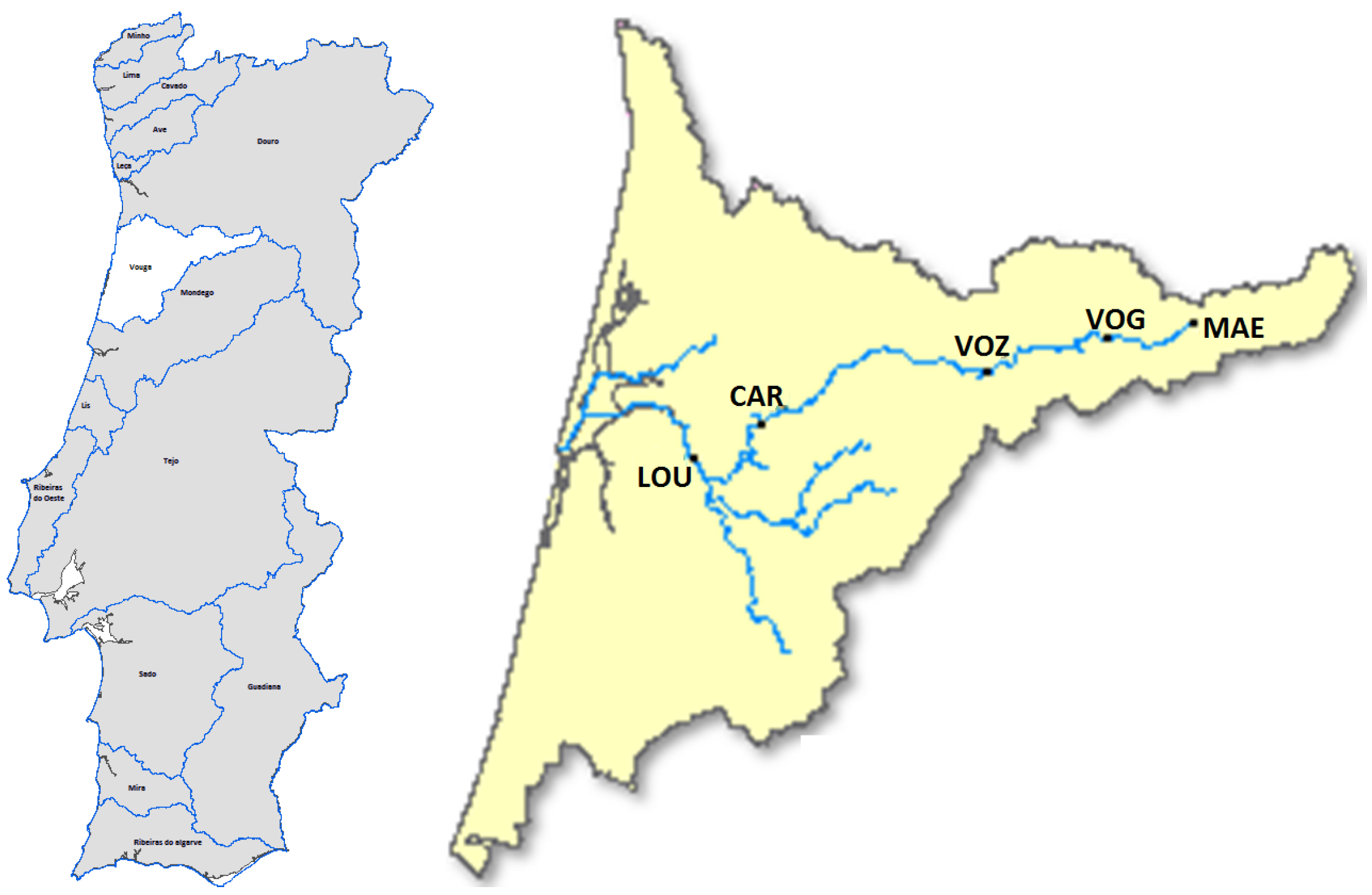
The dataset were collected from the Portuguese National Information System for Water Resources, SNIRH [31].

Table 1. Descriptive statistics of dissolved oxygen concentration between January 2002 and May 2013.

Monitoring Site	Abbrev	Alt. (m)	Lat. (N)	Long. (W)	Obs	Min	Max	Average	St Dev
Ponte São João de Loure	LOU	7	40.6268	−8.54329	112	5.4	11.0	8.24	1.25
Carvoeiro	CAR	18	40.68092	−8.43493	112	6.2	11.0	8.79	1.18
Ponte Vouzela	VOZ	161	40.73985	−8.09383	109	3.2	13.0	8.10	1.91
Vouguinha	VOG	441	40.75775	−7.89324	114	5.4	11.0	8.42	1.35
Aç. Maeira	MAE	495	40.7731	−7.79432	115	5.6	11.0	8.50	1.20

Alt.—altitude, Lat.—latitude, Long.—Longitude, obs.—number of monthly measurements in each water monitoring site, min—minimum, max—maximum, st dev—standard deviation.

lists the information about the water monitoring sites and the respective descriptive statistics of the DO concentration for the modeling period and Figure 1 presents the location of the Vouga river watershed in Portugal and also the monitoring sites locations along Vouga river. Descriptive statistics show that the monitoring site of Ponte Vouzela (VOZ) has the highest sample standard deviation and the smallest sample mean. These values indicate a greater variability of the DO in this site compared to the others. One possible reason is the activity of the poultry and lagomorph slaughterhouses; the lowest DO concentration mean level may be associated with pollutant discharge into the waterways [13]. However, the analysis of these sample statistics must be prudent, since data have a time correlation and, possibly, they are a non-stationary times series.

Since the original data had some months with more than one measurement, their average was taken for those months. Furthermore, there are some missing values in the original dataset. In the period up to May 2013, the percentage of missing values ranged from 16% up to 20%, while, in the remaining period up to May 2015, these percentages are larger. The missing values in the modeling period were filled as specified in [13], who used the same data for other goals.

2.2. Methods

2.2.1. Competitive Models

In each water monitoring site, different time series models were proposed in order to analyze the monthly values of DO concentration from both modeling and forecast frameworks. Three different models were considered: a linear regression model (basis model), a linear regression model with autoregressive errors, and a calibration model with a state-space structure. The last two models are considered improved versions of the linear regression model.

• Linear regression model (MI)

Given the seasonal behavior of the DO concentration, we considered a linear regression model that takes into account the seasonal behavior during the year and allows different growth rates of DO according to the month. That is, the model incorporates 12 slopes and 12 intercepts, and it can be written as:

$$\begin{array}{ccc}\hfill Y_t& =& ({\alpha }_1·t+{\beta }_1)I_{t,1}+({\alpha }_2·t+{\beta }_2)I_{t,2}+\dots +({\alpha }_{12}·t+{\beta }_{12})I_{t,12}+{\xi }_t\hfill \\ & =& \sum _{s=1}^{12}({\alpha }_s·t+{\beta }_s)I_{t,s}+{\xi }_t,\hfill \end{array}$$

(1)

where $Y_t$ is the DO concentration in the month t; ${\alpha }_s$ and ${\beta }_s$, with $s=1,2,\dots ,12$, are, respectively, the slope parameter and the intercept coefficient associated with the month $t=s+12k$, for $k=0,1,2,\dots$. The indicator function $I_{t,s}$ is defined such that $I_{t,s}=1$ if $t=s+12k$, for $k=0,1,2,\dots$, and $I_{t,s}=0$ otherwise, and the error component, ${\xi }_t$, is a white noise process such that $E\left({\xi }_t\right)=0$, $var\left({\xi }_t\right)={\sigma }_{\xi }^2$, $E\left({\xi }_t{\xi }_r\right)=0$ for $t\ne r$. For this model, the ordinary least squares (OLS) method was performed to estimate model parameters. Note that in the case of normal errors, the least square estimation corresponds to the maximum likelihood estimation.

The basis linear regression model is very versatile, in the sense that it incorporates 12 simple linear regression models, where the independent variable is time, t, considering a unique white noise process to model the stochastic component.

• Linear regression model with autoregressive errors (MII)

While, in the previous model, the error components are assumed to be serially uncorrelated, this model considers that the error component has a correlation structure according to an autoregressive process of order one, ${\xi }_t\sim \mathrm{AR}\left(1\right)$, as follows:

$$\begin{array}{ccc}\hfill Y_t& =& \sum _{s=1}^{12}({\alpha }_s·t+{\beta }_s)I_{t,s}+{\xi }_t\hfill \end{array}$$

(2)

$$\begin{array}{ccc}\hfill {\xi }_t& =& \varphi {\xi }_{t-1}+a_t,\hfill \end{array}$$

(3)

where $a_t$ is a Gaussian white noise process ($E\left(a_t\right)=0$, $var\left(a_t^2\right)={\sigma }_a^2$, $E\left(a_t{a}_r\right)=0$, and $a_t\sim N(0,{\sigma }_a^2)$, for $t\ne r$; $\varphi$ is the autoregressive parameter; and ${\sigma }_a^2$ is the variance of the process $\left\{a_t\right\}$.

Note that, in this case, and assuming that $\left|\varphi \right|<1$, the AR(1) process $\left\{{\xi }_t\right\}$ is a stationary process—that is, $E\left({\xi }_t\right)=0$ and $var\left({\xi }_t\right)={\sigma }_a^2/(1-{\varphi }^2)$.

Note that, in linear regression models, it is commonly assumed that the distribution of the errors in the model is Gaussian. This assumption, along with the non-correlation of errors assumption, has to be assessed after parameter estimation in order to ensure the model’s validity. These evaluations were made using standard statistical tests. One way of estimating model parameters is by applying the decomposition method, i.e., firstly, the regression parameters are estimated through least squares method, and then, using the same method, the estimation of parameters associated with the AR(1) component is performed. In this second step, it is considered a linear regression model without intercept, where ${\xi }_t$ is the dependent variable and ${\xi }_{t-1}$ is the independent variable.

Usually, different software presents the linear model parameter estimates with the respective p-values, which are computed assuming uncorrelated errors. Since, in this model, the process of errors, $\left\{{\xi }_t\right\}$, follows an AR(1) process, the p-values associated with the regression coefficients must be corrected in order to correctly identify the statistically significant parameters of the model. The corrected p-values can be computed following the work of [32]. In that work, authors showed that the vector of OLS estimators is asymptotically normal with variance/covariance matrix, given by:

$$Var\left(\widehat{\mathit{\beta }}\right)={\widehat{\sigma }}_a^2{\left[\mathbf{\Phi }\left(B\right){\mathit{X}}^{\prime }\mathbf{\Phi }\left(B\right)\mathit{X}\right]}^{-1}$$

(4)

where $\mathit{X}$ represents the design matrix and $\mathbf{\Phi }\left(B\right)$ represents the matrix, where each element is obtained by applying the operator $\mathbf{\Phi }\left(B\right)$ to the corresponding element of the matrix $\mathit{X}$, that is,

$$x_{t,j}^{\ast }=\mathbf{\Phi }\left(B\right)x_{t,j}=x_{t,j}-\varphi x_{t-1,j}.$$

Although parameters $\varphi$ and ${\sigma }_a^2$ are unknown, they may be replaced by consistent estimators. This allows asymptotic tests for the significance of each variable based on the normal distribution (z-test) [33].

• Calibration model (MIII)

The calibration model assumes a stochastic calibration factor for calibrating the regression base model, which is more flexible than the previous basis model. This model is a state-space representation, in the form:

$$\begin{array}{ccc}\hfill Y_t& =& \left(\sum _{s=1}^{12}({\alpha }_s·t+{\beta }_s)I_{t,s}\right)·X_t+e_t\hfill \end{array}$$

(5)

$$\begin{array}{ccc}\hfill X_t& =& \mu +\varphi (X_{t-1}-\mu )+{\epsilon }_t.\hfill \end{array}$$

(6)

Equation (5) is the observation equation, with $\left(e_t\right)$ being a white noise process, called the observation error, and Equation (6) is the state equation, where $\left\{X_t\right\}$ is the calibration factor process, which is assumed to be a stationary autoregressive process with mean $\mu$ and with an autoregressive parameter $\left|\varphi \right|<1$; ${\epsilon }_t$ is the state error that is also assumed to be a white noise process that is uncorrelated with the observation error process, that is, $E\left(e_t{\epsilon }_r\right)=0$, $\forall t,r$. It is worth mentioning that the assumptions stated here have to be evaluated in order to validate the model. In this case, it is also necessary to evaluate the stationarity of the calibration factor process through the analysis of the $\varphi$ estimate and its standard error.

The model has two main components: a regression structure, which incorporates both trend and seasonality, and an unobservable process, the calibration factor, the state. It can be seen in Equation (5) that the state process will calibrate the deterministic structure. The state-space model has in its structure a latent process, the state, which is not observable and must be predicted. The most common procedure to make this prediction is the Kalman filter algorithm [34,35]. This procedure computes, at each moment t, the optimal estimator of the state vector based on the information available up to that time t. The Kalman filter’s success lies in the fact that it is an online estimation procedure. When the errors and the initial state $X_1$ are Gaussian, the predictors of the Kalman filter are the best unbiased estimators, with respect to the minimum mean square error. However, optimum properties can only be guaranteed when all parameters of model are known [36]. When parameters of the state-space model have to be estimated, the uncertainty associated with Kalman’s filter estimators is underestimated, and some procedures can be implemented [35]. Hence, the parameters of the model can be estimated using the maximum likelihood (ML) method, incorporating the Kalman filter algorithm, and numerical procedures, such as Newton–Raphson, in order to achieve the optimal value of the likelihood.

The parameters of model (5) and (6) will be estimated by applying a decomposition approach, taking into account the main components previously identified. In the first stage, the OLS method is used to estimate the parameters of the deterministic regression structure that will be considered, known as the state parameter estimation stage. In practice, the first stage is the estimation procedure performed in model MII (2) and (3).

Models MII (2), (3) and MIII (5), (6) can be seen as improved versions of the simple linear regression model MI, but more flexible and allowing the capture of more elaborate dynamics of the underlying process. Both models have a regression component that will be estimated with the same procedure.

2.2.2. Model Performance Measures

In order to evaluate each of the proposed models, we evaluated not only the behavior of each model within the estimation period, but also their predictive ability. In the first situation, we considered the coefficient of determination $R^2$, the mean square error (MSE), the mean absolute error (MAE), and the mean percentage absolute error (MPAE); in the forecast framework, only considered the last three measures were considered.

The above performance measures are the most commonly used in time series analysis. The coefficient of determination is the linear correlation between observations and the correspondent model estimates, and it allows the evaluatation of the models’ adequacy. Furthermore, while MSE is a quadratic measure, MAE is a measure with the advantage of using the same units as the observations. MPAE is a useful measure when the comparisons made are in different units, since is dimensionless. The formulae of the measures to evaluate model performance are listed in

Table 2. Model performance measures.

	In Sample	Prediction
$R^2$	${\mathrm{Corr}}^2(Y_t,{\widehat{Y}}_t)$	-
$\mathrm{MSE}$	${\displaystyle \frac{1}{n}\sum _{t=1}^n{(Y_t-{\widehat{Y}}_t)}^2}$	${\displaystyle \frac{1}{\#H}\sum _{h\in H}{(Y_{n+h}-{\widehat{Y}}_{n+h})}^2}$
$\mathrm{MAE}$	${\displaystyle \frac{1}{n}\sum _{t=1}^n|Y_t-{\widehat{Y}}_t|}$	${\displaystyle \frac{1}{\#H}\sum _{h\in H}|Y_{n+h}-{\widehat{Y}}_{n+h}|}$
$\mathrm{MPAE}$	${\displaystyle \frac{1}{n}\sum _{t=1}^n\frac{|Y_t-{\widehat{Y}}_t|}{|Y_t|}}$	${\displaystyle \frac{1}{\#H}\sum _{h\in H}\frac{|Y_{n+h}-{\widehat{Y}}_{n+h}|}{|Y_{n+h}|}}$

, where ${\widehat{Y}}_t$ is the estimate of the DO at time t, n is the length of the time series used for modeling, and H is the set of indices of h-step ahead, such that there is a DO concentration observation, $Y_{n+h}$.

Note that the estimate of the DO concentration at time t, ${\widehat{Y}}_t$, depends on the model we are working with. Assuming that all parameters of the models are statistically significant (if not, its term is not considered in the sum), in a linear regression model, ${\widehat{Y}}_t$ is calculated through the following expression:

$${\widehat{Y}}_t=\sum _{s=1}^{12}({\widehat{\alpha }}_s·t+{\widehat{\beta }}_s)I_{t,s},$$

while, in the linear model with autoregressive errors, one has to apply the formula:

$${\widehat{Y}}_t=\sum _{s=1}^{12}({\widehat{\alpha }}_s·t+{\widehat{\beta }}_s)I_{t,s}+\widehat{\varphi }{\widehat{\xi }}_{t-1},$$

where ${\widehat{\xi }}_t$ is the residual of the regression component, and it is assumed that ${\widehat{\xi }}_1=0$. For the calibration model MIII (5)–(6), the estimate of the DO concentration is the one-step ahead forecast estimate that can be computed through:

$${\widehat{Y}}_t=\left(\sum _{s=1}^{12}({\widehat{\alpha }}_s·t+{\widehat{\beta }}_s)I_{t,s}\right)·{\widehat{X}}_{t|t-1},$$

with ${\widehat{X}}_{t|t-1}$ being the one-step ahead forecast of the calibration factor obtained by the Kalman filter algorithm using the estimated parameters.

Concerning the h-step ahead forecast, in the model MI, the forecast ${\widehat{Y}}_{n+h}$ is obtained with a straightforward adaptation of the estimate expression ${\widehat{Y}}_t$. For model MII (2)–(3), since the last estimated error is at time n, recursively, the h-step ahead forecast estimate can be computed through the formula:

$${\displaystyle {\widehat{Y}}_{n+h}=\sum _{s=1}^{12}\left({\widehat{\alpha }}_s·(n+h)+{\widehat{\beta }}_s\right)I_{n+h,s}+{\widehat{\varphi }}^h{\widehat{\xi }}_n.}$$

In model MIII (5)–(6), it is necessary to predict the state at time $n+h$, $X_{n+h}$, using the prediction of the state at time n, ${\widehat{X}}_{n+h|n}$, through the expression

$${\widehat{X}}_{n+h|n}=\widehat{\mu }+{\widehat{\varphi }}^h({\widehat{X}}_{n|n}-\widehat{\mu }),$$

which is used to estimate $Y_{n+h}$,

$${\widehat{Y}}_{n+h}=\left({\displaystyle \sum _{s=1}^{12}\left({\widehat{\alpha }}_s·(n+h)+{\widehat{\beta }}_s\right)I_{n+h,s}}\right)·{\widehat{X}}_{n+h|n}.$$

3. Results

Since the DO concentration series has a seasonal behavior, at a preliminary stage, we considered a linear regression model (MI) that accounts for the seasonal behavior of the DO concentration during the year, as well as for the increase in DO concentration that may occur at different rates according to the month.

Table 3. Results for the MI model for dissolved oxygen (DO) concentration at the different locations.

	LOU			CAR			VOZ			VOG			MAE
	est.	p-val.	p-val. *	est.	p-val.	p-val. *	est.	p-val.	p-val. *	est.	p-val.	p-val. *	est.	p-val.	p-val. *
${\alpha }_1$	0.007	0.20	0.26	0.002	0.77	0.80	−0.004	0.60	0.65	0.000	0.95	0.96	−0.002	0.75	0.78
${\alpha }_2$	−0.004	0.42	0.43	−0.002	0.68	0.69	0.002	0.79	0.79	0.001	0.89	0.89	0.000	0.94	0.94
${\alpha }_3$	−0.004	0.41	0.41	−0.006	0.32	0.33	−0.004	0.56	0.56	−0.003	0.63	0.63	−0.002	0.69	0.69
${\alpha }_4$	0.001	0.92	0.92	0.000	0.95	0.95	−0.003	0.68	0.68	0.003	0.64	0.64	0.000	0.95	0.95
${\alpha }_5$	−0.007	0.16	0.17	−0.010	0.09	0.09	0.003	0.68	0.68	0.000	0.96	0.96	−0.002	0.71	0.72
${\alpha }_6$	−0.011	0.06	0.06	−0.004	0.60	0.59	−0.004	0.64	0.64	−0.003	0.67	0.67	−0.002	0.71	0.71
${\alpha }_7$	−0.004	0.46	0.46	−0.009	0.16	0.16	0.001	0.86	0.86	−0.018	0.01	0.01	−0.008	0.23	0.24
${\alpha }_8$	−0.006	0.33	0.33	0.007	0.30	0.31	0.005	0.55	0.56	−0.012	0.08	0.08	−0.013	0.05	0.05
${\alpha }_9$	−0.011	0.06	0.06	0.005	0.46	0.47	0.011	0.18	0.17	−0.011	0.11	0.11	0.000	0.98	0.98
${\alpha }_{10}$	−0.005	0.45	0.45	−0.001	0.93	0.93	−0.012	0.15	0.15	−0.008	0.25	0.25	−0.006	0.34	0.34
${\alpha }_{11}$	−0.004	0.47	0.47	−0.006	0.40	0.40	−0.016	0.05	0.05	−0.014	0.03	0.03	−0.010	0.13	0.13
${\alpha }_{12}$	−0.002	0.78	0.78	0.000	0.94	0.94	0.004	0.61	0.62	−0.003	0.70	0.71	−0.002	0.76	0.76
${\beta }_1$	9.247	0.00	0.00	10.094	0.00	0.00	11.109	0.00	0.00	10.537	0.00	0.00	10.190	0.00	0.00
${\beta }_2$	9.887	0.00	0.00	10.147	0.00	0.00	9.547	0.00	0.00	9.502	0.00	0.00	9.532	0.00	0.00
${\beta }_3$	9.513	0.00	0.00	9.947	0.00	0.00	9.425	0.00	0.00	9.698	0.00	0.00	9.737	0.00	0.00
${\beta }_4$	8.715	0.00	0.00	9.001	0.00	0.00	9.559	0.00	0.00	8.944	0.00	0.00	9.014	0.00	0.00
${\beta }_5$	8.839	0.00	0.00	9.262	0.00	0.00	8.347	0.00	0.00	8.709	0.00	0.00	8.753	0.00	0.00
${\beta }_6$	8.362	0.00	0.00	8.005	0.00	0.00	7.518	0.00	0.00	8.032	0.00	0.00	7.939	0.00	0.00
${\beta }_7$	7.572	0.00	0.00	8.793	0.00	0.00	7.175	0.00	0.00	8.576	0.00	0.00	8.376	0.00	0.00
${\beta }_8$	7.491	0.00	0.00	8.377	0.00	0.00	6.231	0.00	0.00	7.668	0.00	0.00	8.260	0.00	0.00
${\beta }_9$	7.971	0.00	0.00	7.604	0.00	0.00	5.056	0.00	0.00	7.922	0.00	0.00	7.319	0.00	0.00
${\beta }_{10}$	7.730	0.00	0.00	7.883	0.00	0.00	8.489	0.00	0.00	8.105	0.00	0.00	8.477	0.00	0.00
${\beta }_{11}$	8.343	0.00	0.00	9.371	0.00	0.00	9.737	0.00	0.00	9.673	0.00	0.00	9.408	0.00	0.00
${\beta }_{12}$	9.979	0.00	0.00	9.912	0.00	0.00	9.124	0.00	0.00	9.208	0.00	0.00	9.207	0.00	0.00
$R^2$	0.727			0.628			0.713			0.713			0.627
$\varphi$	0.327	0.00		0.388	0.00		0.162	0.06		0.290	0.00		0.342	0.00
${\sigma }_a^2$	0.519			0.606			1.018			0.652			0.642

* Corrected p-value according to the errors autocorrelation, Equation (4).

presents the ordinary least squares (OLS) estimates obtained in the adjustment of the above-described linear model (MI) of the monthly DO concentration data for the water monitoring sites under study.

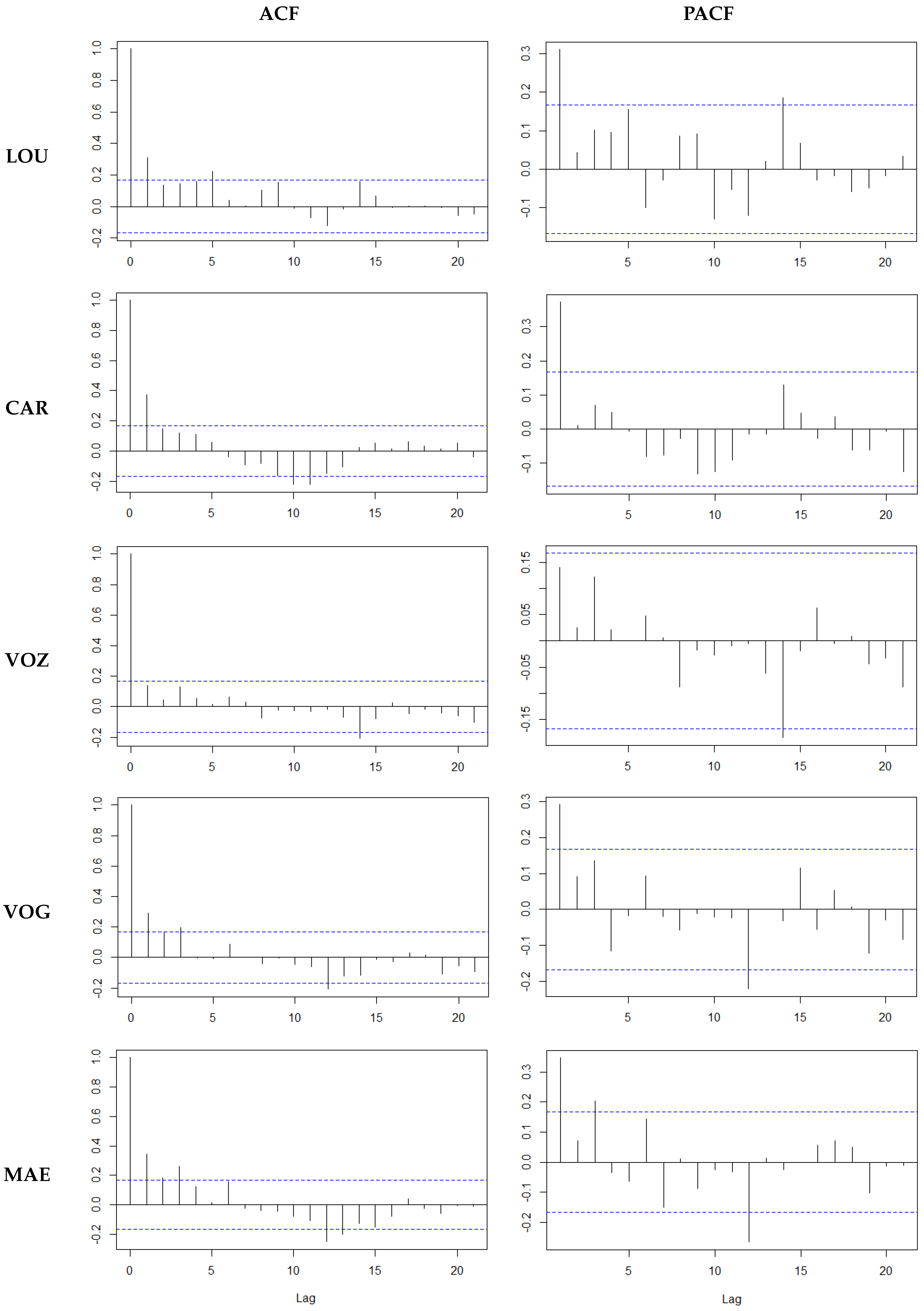
For each location, the estimates of the coefficients and the respective p-values, as well as the determinant coefficient values, $R^2$, are presented. The data indicate a good fit for all five models. Moreover, for all series, the residual series of the adjusted model MI presents a weak time correlation. In fact, if the linear model fits well to data, the residual series has white noise behavior, that is, both the sample autocorrelation function (ACF) and the sample partial autocorrelation function (PACF) have values statistically insignificant at a 5% level. The time correlation structure can be generally described by an autoregressive processes of order 1, AR(1), as can be seen from the analysis of the ACF and the PACF displayed in Figure 2, due to the ACF decreasing exponentially to zero, while the PACF has a significant value on lag 1. So, in order to assess the statistically significant parameters, the corrected p-values are also presented in Table 3, as well as the AR(1) parameter estimates considered in the p-values correction.

From the analysis of the estimation results, for each monitoring site, the estimates of all intercepts are statistically significant, considering a significance level of 10%. For monthly slopes, at least one parameter estimate is statistically significant for each monitoring site model. In the LOU station series, significant slope parameters are associated with June and September. In the CAR monitoring site is a significant slope parameter for May, while, in VOZ, it is the November slope parameter. In the VOG site model case, the significant slope parameters are associated with July, August, and November, and in the model of station MAE, only the August slope parameter is statistically significant. Note that all significant slope estimates are negative, indicating that, during those months, DO concentration was decreasing.

Due to the existence of temporal correlation in the residues, the MI model is not adequate to describe the behavior of the underlying process, so the MII (2)–(3) and MIII (5)–(6) models were used as possible alternatives. Furthermore, only significantly monthly slopes in Table 3 were considered in these models.

Table 4. Results for model MII (2)–(3) for DO concentrations at the different locations.

	LOU			CAR			VOZ			VOG			MAE
	est.	p-val.	p-val. *	est.	p-val.	p-val. *	est.	p-val.	p-val. *	est.	p-val.	p-val. *	est.	p-val.	p-val. *
${\alpha }_5$				−0.010	0.09	0.06
${\alpha }_6$	−0.011	0.06	0.04
${\alpha }_7$										−0.018	0.01	0.01
${\alpha }_8$										−0.012	0.07	0.06	−0.013	0.05	0.02
${\alpha }_9$	−0.011	0.06	0.04
${\alpha }_{11}$							−0.016	0.01	0.05	−0.014	0.01	0.02
${\beta }_1$	9.703	0.00	0.00	10.209	0.00	0.00	10.862	0.00	0.00	10.512	0.00	0.00	10.190	0.00	0.00
${\beta }_2$	9.599	0.00	0.00	9.983	0.00	0.00	9.673	0.00	0.00	9.559	0.00	0.00	9.532	0.00	0.00
${\beta }_3$	9.212	0.00	0.00	9.546	0.00	0.00	9.138	0.00	0.00	9.504	0.00	0.00	9.737	0.00	0.00
${\beta }_4$	8.753	0.00	0.00	9.001	0.00	0.00	9.356	0.00	0.00	9.134	0.00	0.00	9.014	0.00	0.00
${\beta }_5$	8.313	0.00	0.00	9.262	0.00	0.00	8.555	0.00	0.00	8.688	0.00	0.00	8.753	0.00	0.00
${\beta }_6$	8.362	0.00	0.00	7.771	0.00	0.00	7.270	0.00	0.00	7.847	0.00	0.00	7.939	0.00	0.00
${\beta }_7$	7.273	0.00	0.00	8.164	0.00	0.00	7.271	0.00	0.00	8.576	0.00	0.00	8.376	0.00	0.00
${\beta }_8$	7.087	0.00	0.00	8.844	0.00	0.00	6.556	0.00	0.00	7.668	0.00	0.00	8.260	0.00	0.00
${\beta }_9$	7.971	0.00	0.00	7.941	0.00	0.00	5.800	0.00	0.00	7.166	0.00	0.00	7.319	0.00	0.00
${\beta }_{10}$	7.410	0.00	0.00	7.844	0.00	0.00	7.673	0.00	0.00	7.561	0.00	0.00	8.477	0.00	0.00
${\beta }_{11}$	8.030	0.00	0.00	8.968	0.00	0.00	9.737	0.00	0.00	9.673	0.00	0.00	9.408	0.00	0.00
${\beta }_{12}$	9.859	0.00	0.00	9.946	0.00	0.00	9.418	0.00	0.00	9.025	0.00	0.00	9.207	0.00	0.00
$R^2$	0.705			0.598			0.691			0.695			0.606
$\varphi$	0.311	0.00		0.372	0.00		0.140	0.06		0.292	0.00		0.348	0.00
${\sigma }_a^2$	0.514			0.594				0.980			0.629			0.608

* Corrected p-value according to error autocorrelation, Equation (4).

presents the OLS estimates of the parameters of model MII (2)–(3). Note that monthly slope estimates are all negative values, indicating that, in these cases, there are decreasing trends in those months. Furthermore, note that the months with the lowest intercept estimated values are, in the majority of the location sites, the summer months, and it is in the VOZ location that the lowest values can be found.

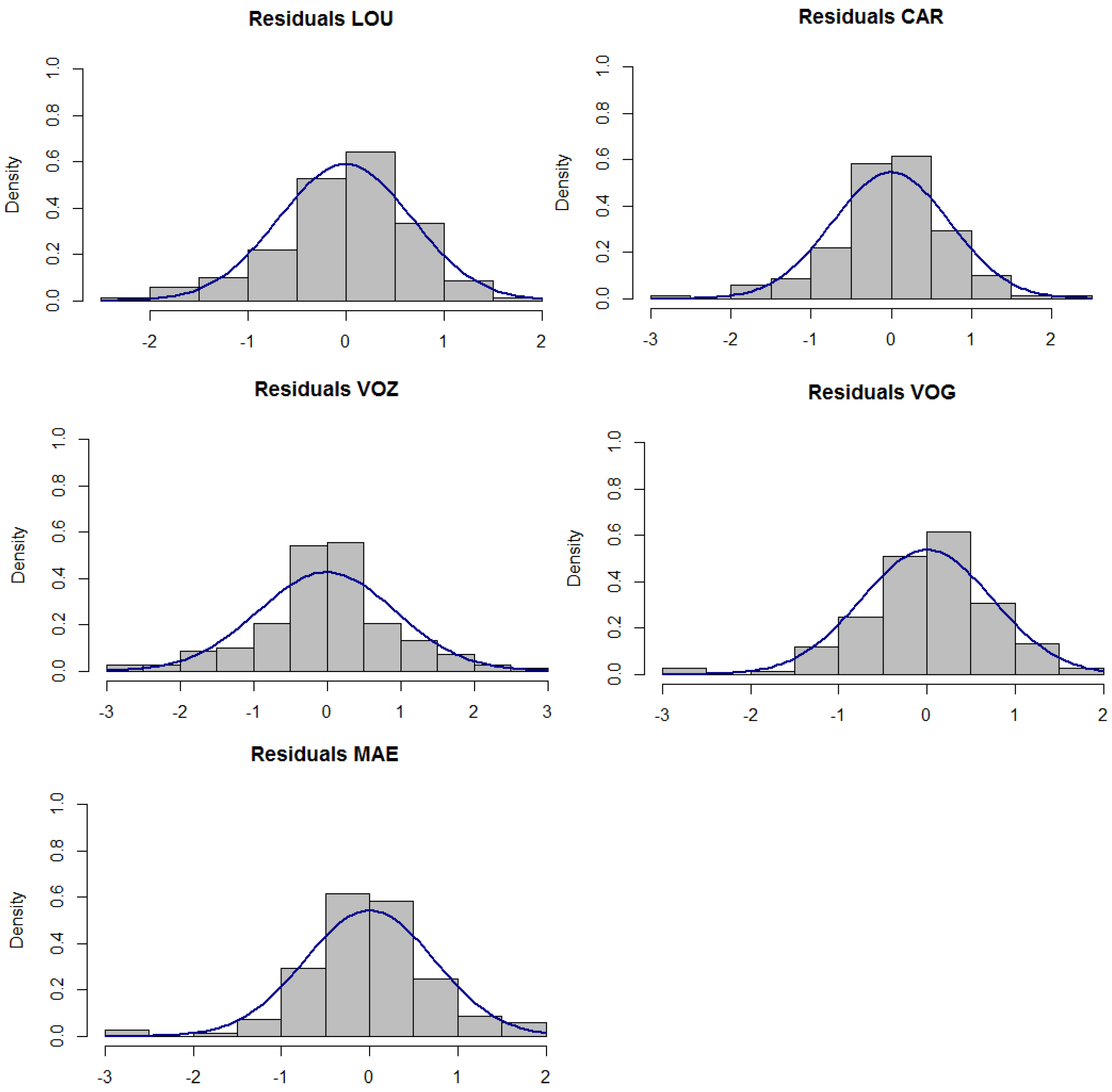
For the model MII (2)–(3), the residuals of the models did not present a significant time correlation; their histograms, after applying the Lunj-Box test with different lags, can be seen in Figure 3. The graphs do not seem to be far from the normal curve and, with the exception of the CAR monitoring site, they do not reject the normality assumption at the 1% significance level through the Kolmogorov–Smirnov test (K–S). This test is usually applied when the series dimension is large. The Jarque–Bera test, which compares the empirical skewness and kurtosis with the correspondent Gaussian values, was also applied, and the results pointed in the same direction: residuals normality was not rejected.

Regarding the calibration model MIII (5)–(6), the parameters of the regression component were already estimated using OLS (Table 4), and they were considered as known in order to apply the ML method to estimate the parameters associated with the calibration process. Hence, for each monitoring site, estimation results are presented in

Table 5. Estimation results for the calibration model MIII (5)–(6).

Site	$\mathit{\mu }$		$\mathit{\varphi }$		${\mathit{\sigma }}_{\mathit{\epsilon }}^2·{10}^{-3}$		${\mathit{\sigma }}_{\mathit{e}}^2$			K-S
	Coeff.	Std. Error	Coeff.	Std. Error	Coeff.	Std. Error	Coeff.	Std. Error	${\mathit{R}}^{\mathbf{2}}$	p-val.
LOU	0.9996	0.0012	0.8300	0.0106	0.6516	0.0506	0.3591	0.0055	0.705	0.0240
CAR	1.0001	0.0010	0.5940	0.0155	2.881	0.1605	0.2662	0.0107	0.596	0.0035
VOZ	1.0005	0.0010	0.7932	0.0112	0.5274	0.0614	0.7898	0.0116	0.698	0.1800
VOG	0.9996	0.0011	0.6765	0.0162	1.7245	0.1232	0.3724	0.0088	0.701	0.0228
MAE	0.9990	0.0012	0.7233	0.0126	1.7907	0.1036	0.3390	0.0077	0.616	0.0246

, along with the coefficients of determination. These values are, with the exception of the LOU station, equal to or slightly better than the calibration models. As expected, the state processes are all stationary, with means around one, since, accounting for the respective standard errors, all estimates of $\varphi$ are less then one.

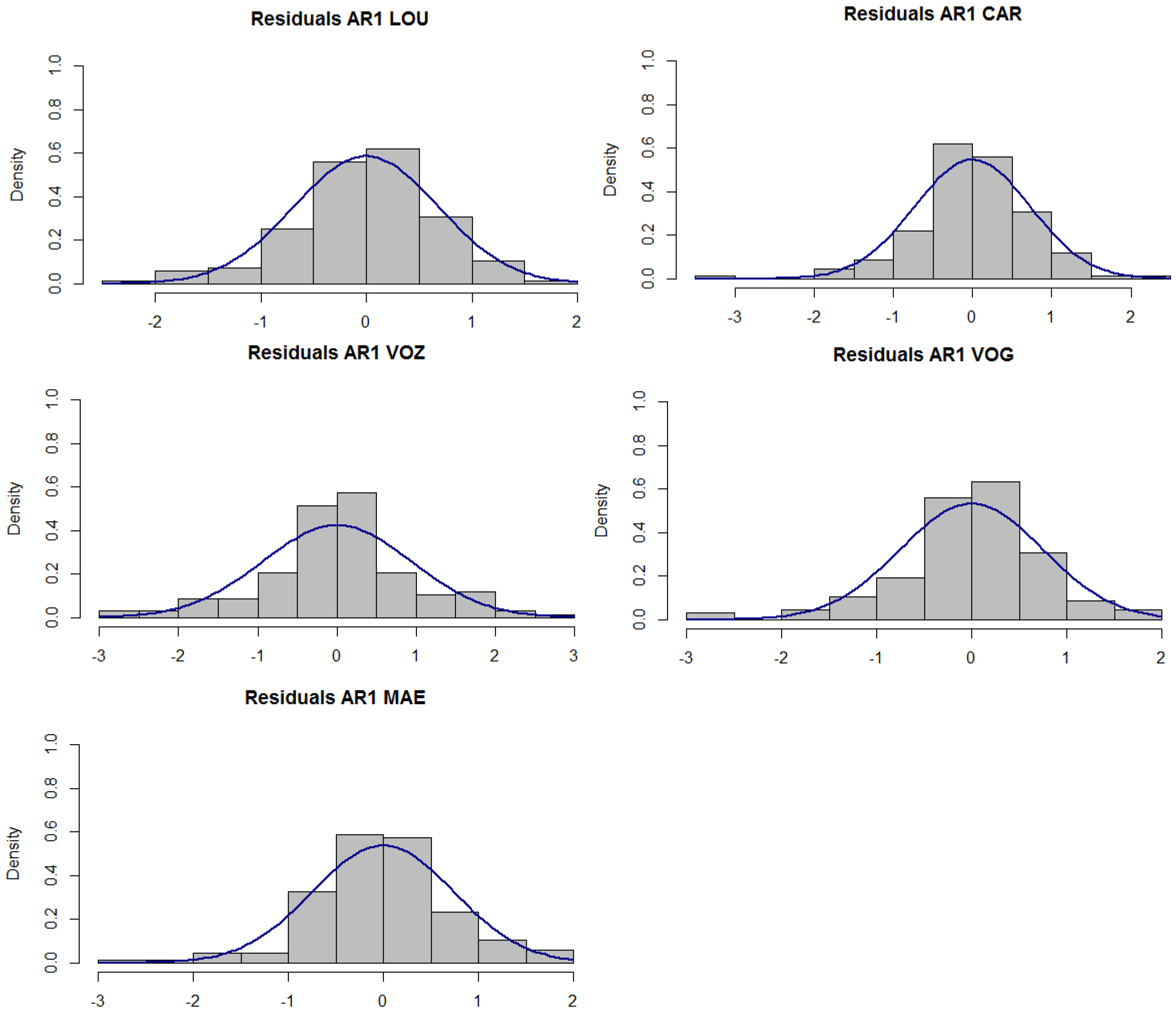
Concerning the residual analysis, both sample ACF and PACF of the residual series have behavior similar to white noise. In fact, the Lunj-Box test for the non-correlation hypothesis does not reject, using up to 30 different lags in all the locations under study, and Figure 4 presents the histograms of the residuals that resemble the normal curve.

Furthermore, with the exception of the CAR location, the residuals of the calibration model do not reject (at a 1% significance level) the normality assumption using the Jarque–Bera test or the Kolmogorov–Smirnov test; the K–S p-values are presented in Table 5.

4. Discussion

The models proposed have different statistical properties, since they can be applied according to the analysis’s objectives. In fact, mainly models MII (2)–(3) and MIII (5)–(6), which were statistically validated, assume that the time correlation is incorporated in the linear model in different ways, despite both models considering an autoregressive model of order 1.

In the case of model MII (2)–(3), the process AR(1) is additive, that is, the time-dependence is added to the deterministic component, which is based on a linear regression model. This approach considers that time correlation is not influenced by the deterministic component (trend and seasonality), it only incorporates the past as a Markovian variable, in the sense that time t only depends on the last value in time $t-1$.

Model III (5)–(6) has the same deterministic component of trend and seasonality as model MII, but, in this case, the autoregressive process $X_t\sim AR\left(1\right)$ is incorporated as a factor, that is, in a multiplicative way. In this case, the mean value of the process $X_t$ is 1. So, the process $X_t$ can be interpreted as an index, where a value ${\xi }_t$ less than 1 means that, in that month, the measurement of the water quality variable is $(1-X_t)\times 100\%$ lower than the expected value based on the deterministic component. If $X_t$ assumes a value greater than 1, in that month, the observed value is $(X_t-1)\times 100\%$ greater than the expected value, based on the deterministic component. This interpretation allows us to identify the model MIII as a calibration model.

Thus, models II and III have the same basis model which incorporates trend and seasonal components, but they incorporate the time correlation in different ways, thus allowing different interpretations and information.

Based on empirical data, model comparison is performed from two points of view: predictions one-step ahead in sample, and h-step ahead forecasts in future accuracy. However, as the model MI, the basis model, was not validated from the statistical point of view, and since the residual series has serial correlation, only models MII (2)–(3) and MIII (5)–(6) were compared.

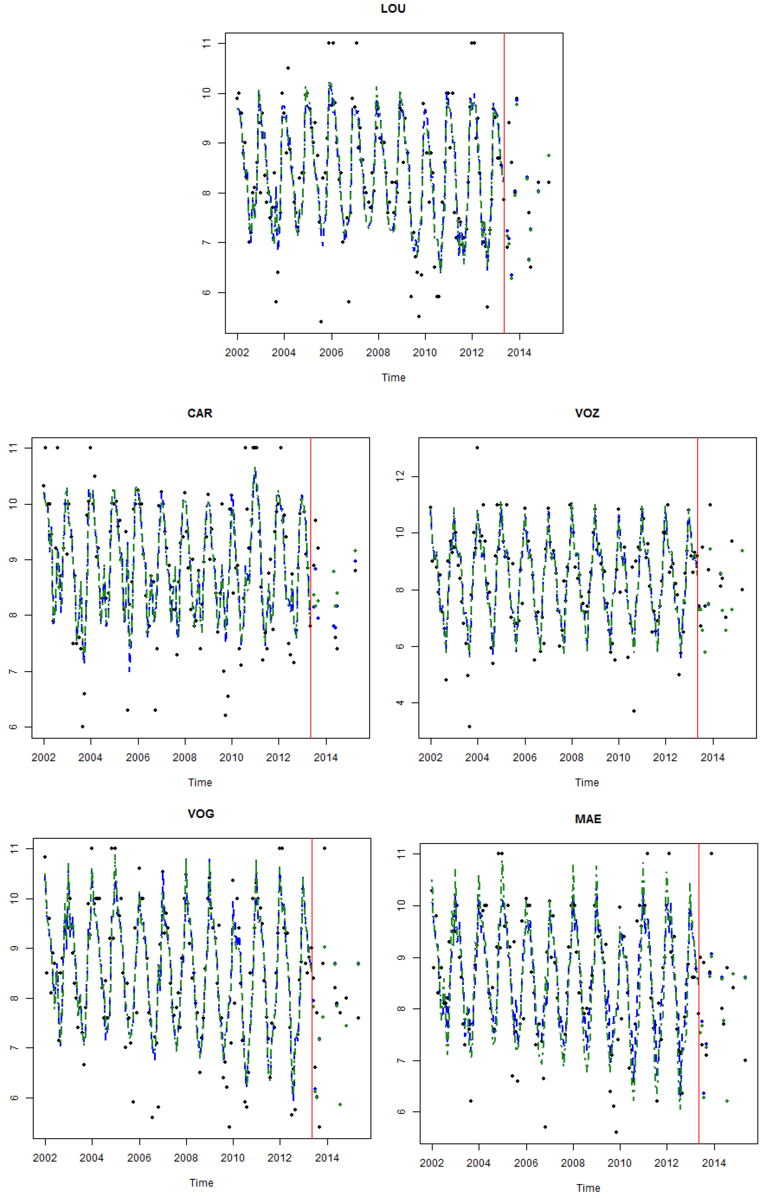
Figure 5 presents graphically, for each DO time series, the observations which correspond to the full period under consideration and the DO predictions—in-sample and forecasted out-of-sample—for both models under analysis. The period from June 2013 to May 2015 was used to evaluate the forecast ability; however, for each site, there are few available values in this period. Globally, both models fit very well in the period of estimation. However, as it was expected, the one-step ahead forecasts in both models did not pick up the extreme values (large or small values), since the linear regression model estimates the conditional expectation of the dependent variable given the independent variables, that is, the average value of the dependent variable when the independent variables are fixed.

Table 6. Mean square error (MSE), in-sample and h-step-ahead forecast, for models MII and MIII.

Site	In Sample		Forecasting
	MII	MIII	MII	MIII	$\#\mathbf{H}$
LOU	0.461	0.460	1.239	1.321	10
CAR	0.528	0.534	0.506	0.850	7
VOZ	0.879	0.867	2.262	2.254	11
VOG	0.555	0.550	1.506	1.527	11
MAE	0.545	0.535	2.035	2.081	11

presents the mean square error (MSE) for each monitoring site for both models MII (2)–(3) and MIII (5)–(6) from the one-step ahead perspective (in-sample) and also from the forecasted point of view. The number of available DO observations in the considered forecast period for each time series is indicated by the $\#H$ column. Therefore, the predictive ability is assessed taking into account only the observed available data, assuming that the last observation (n) is the DO value in May 2013.

In the one-step-ahead in-sample, the considered model MII’s predictions of the DO concentration have an MSE between $0.461$ in LOU and $0.879$ in VOZ. Since MSE is given in squared units, we computed their square root (RMSE), obtaining values between $0.679$ and $0.938$ mg/L. However, these values increase to values of RMSE between $0.711$ and $1.504$ mg/L in the h-ahead forecasts, as expected, since the uncertainty in forecast is greater than in the one-step ahead prediction. These results should be analyzed with caution because the number of observations in the period left of the forecast is reduced.

According to Table 6, with the exception of the CAR location, the calibration model MIII (5)–(6) slightly outperforms the model MII (2)–(3) from a modeling point of view, since this model presents lower MSE values for the other four monitoring sites. However, when it comes to forecasting, the model MII (2)–(3) performs slightly better than the calibration model for all monitoring stations, with the exception of the VOZ location. In this location, the DO concentration series presents greater variability when compared with the other monitoring sites. Since predictions are based on expected values, greater variability increases the difficulty of correctly predicting DO values that are far from the mean value.

These results can be explained by taking into account that the calibration model MIII (5)–(6) assumes a latent process, which is predicted through the Kalman filter algorithm, that is optimal in the filtering procedure. So, model III allows better predictions in an online framework compared to an h-step ahead forecast framework. When there is no additional information, which is the case for the forecast, the calibration model cannot update the state and therefore cannot correctly calibrate the fixed regression component of the model, hence justifying its lower performance when compared with model MII (2)–(3).

In this context, the calibration model MIII with the Kalman filter algorithm can obtain the filtered calibration factors, ${\widehat{X}}_{t|t}$, for each month. These estimates with the associated confidence intervals can be interpreted as indicators of the water monitoring procedure. In fact, considering the empirical $95\%$ confidence intervals:

$$X_t={\widehat{X}}_{t|t}\pm 1.96\sqrt{P_{t|t}}\mathrm{or}{\mathrm{CI}}_{95\%}\left(X_{t|t}\right)=\left[{\widehat{X}}_{t|t}-1.96\sqrt{P_{t|t}},{\widehat{X}}_{t|t}+1.96\sqrt{P_{t|t}}\right]$$

where $P_{t|t}$ is the mean square error obtained by the Kalman filter algorithm.

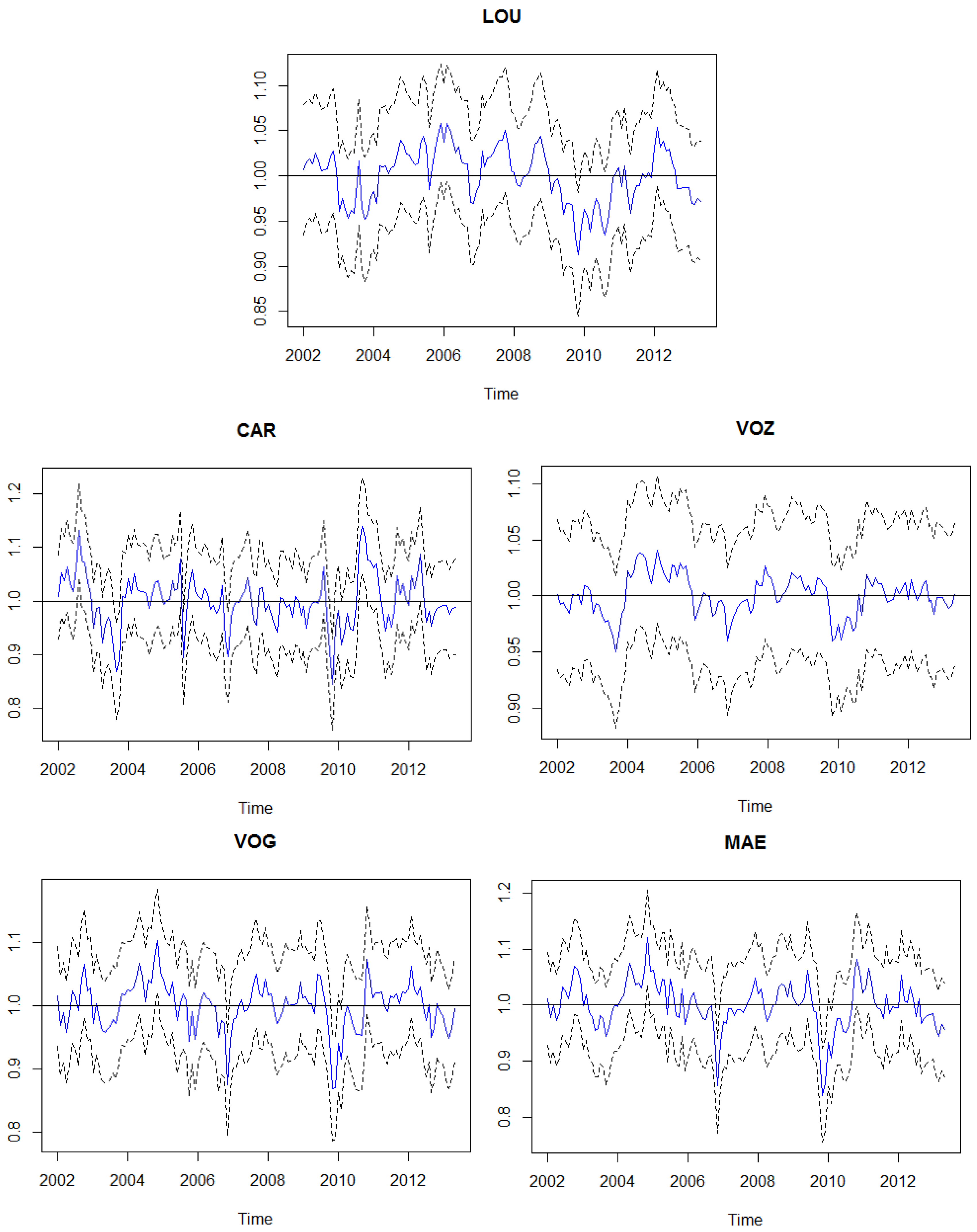
Figure 6 presents filtered estimates of the calibration factor ${\widehat{X}}_{t|t}$ for all site locations with $95\%$ empirical confidence intervals. These intervals can be used for month-to-month evaluatations if the DO concentration measurement is an expected statistical value, considering that if $1\notin {\mathrm{CI}}_{95\%}\left(X_{t|t}\right)$, the measurement is unexpected. So, these procedures can be used in order to identify possible extreme values or exogenous conditions that influence DO concentration. For instance, in the LOU water monitoring site in November 2009 ($t=95$), the calibration factor was estimated to be ${\widehat{X}}_{95|95}=0.913$ but $1\notin {\mathrm{CI}}_{95\%}\left(X_{95|95}\right)=[0.845,0.981]$. So, in this month, the observed DO concentration was $8.7\%$ lower than the expected value for that month, considering trend and seasonality components.

5. Conclusions

Empirical results show that models based on linear regression have good performances when monitoring water quality variables, both in the modeling and in the forecast approach; for instance, in the modeling framework, the coefficients of determination vary approximately from $0.6$ to $0.7$. However, the statistical inference in the regression models has some assumptions that are not verified for the water quality variables. In fact, the monitoring of water quality is often based on a periodic collection of water samples, from which several biochemical variables are analyzed. So, this type of data usually has a time correlation structure that must be incorporated both in model formulation and in inference procedures.

The incorporation of a time series model, as in the AR(1) process, the error process allows a suitable adjustment of models if all assumptions are globally satisfied. Furthermore, this improvement in the initial linear regression model implies an adequate computation of standard errors of the regression parameters, considering that time correlation allows a more accurate statistical procedure. This model is revealed to be more accurate from the forecast point of view.

Additionally, the calibration approach applied to the regression model proves to have a better performance when the main objective is water monitoring using an online approach, favoring the detection of changes in the expected behavior of the variable by interpreting the calibration factor predictions. It is noteworthy that in a certain month t, if the calibration factor prediction ${\widehat{X}}_t$ is less than 1, then, in the correspondent month, the observed value is lower than the expected value based on the analyzed period. The an opposite interpretation applies if ${\widehat{X}}_t$ is greater than 1.

The comparative study of the linear models was based on a DO concentration series, which is considered a good indicator of water status. As topic of future research, it is important to analyze whether the results remain valid for other physical/chemical parameters which are equally important for the characterization of water status. Furthermore, the models under analysis are univariate, hence, a multivariate time series model comparison will be a topic for future research.

References

- Costa, M.; Monteiro, M. Statistical Modelling of Water Quality Time Series—The River Vouga Basin Case Study. In Research and Practices in Water Quality, Modeling and Health Research Methods; Lee, T.S., Ed.; InTech: London, UK, 2015; pp. 149–175. [Google Scholar]
- Hallouin, T.; Bruen, M.; Christie, M.; Bullock, C.; Kelly-Quinn, M. Challenges in Using Hydrology and Water Quality Models for Assessing Freshwater Ecosystem Services: A Review. Geosciences 2018, 8, 45. [Google Scholar] [CrossRef]
- Bhat, S.A.; Meraj, G.; Yaseen, A.; Pandit, A. Statistical Assessment of Water Quality Parameters for Pollution Source Identification in Sukhnag Stream: An Inflow Stream of Lake Wular (Ramsar Site), Kashmir Himalaya. J. Ecosyst. 2014, 2014, 898054. [Google Scholar] [CrossRef]
- Hamid, A.; Bhat, S.; Bhat, S.; Jehangir, J. Environmetric techniques in water quality assessment and monitoring: a case study. Environ. Earth Sci. 2016, 75, 321. [Google Scholar] [CrossRef]
- Shrestha, S.; Muangthong, S. Assessment of surface water quality of Songkhram River (Thailand) using environmetric techniques. Int. J. River Basin Manag. 2014, 12, 341–356. [Google Scholar] [CrossRef]
- Samadi, S.; Tufford, D.; Carbone, G. Estimating hydrologic model uncertainty in the presence of complex residual error structures. Stoch. Environ. Res. Risk Assess. 2018, 32, 1259–1281. [Google Scholar] [CrossRef]
- Barzegar, R.; Asghari Moghaddam, A.; Adamowski, J.; Ozga-Zielinski, B. Multi-step water quality forecasting using a boosting ensemble multi-wavelet extreme learning machine model. Stoch. Environ. Res. Risk Assess. 2018, 32, 799–813. [Google Scholar] [CrossRef]
- Paroissin, C.; Penalva, L.; Pétrau, A.; Verdier, G. New control chart for monitoring and classification of environmental data. Environmetrics 2016, 27, 182–193. [Google Scholar] [CrossRef]
- Lloyd, C.; Freer, J.E.; Collins, A.L.; Johnes, P.J.; Jones, J. Methods for detecting change in hydrochemical time series in response to targeted pollutant mitigation in river catchments. J. Hydrol. 2014, 514, 297–312. [Google Scholar] [CrossRef]
- Arya, F.; Zhang, L. Time series analysis of water quality parameters at Stillaguamish River using order series method. Stoch. Environ. Res. Risk Assess. 2015, 29, 227–239. [Google Scholar] [CrossRef]
- Gonçalves, A.M.; Alpuim, T. Water quality monitoring using cluster analysis and linear models. Environmetrics 2011, 22, 933–945. [Google Scholar] [CrossRef]
- Gonçalves, A.M.; Costa, M. Application of Change-Point Detection to a Structural Component of Water Quality Variables. In AIP Conference Proceedings; American Institute of Physics: Halkidiki, Greece, 2011; pp. 1565–1568. [Google Scholar] [Green Version]
- Costa, M.; Monteiro, M. Discrimination of water quality monitoring sites in River Vouga using a mixed-effect state space model. Stoch. Environ. Res. Risk Assess. 2016, 30, 607–619. [Google Scholar] [CrossRef] [Green Version]
- Costa, M.; Goncalves, A. Clustering and forecasting of dissolved oxygen concentration on a river basin. Stoch. Environ. Res. Risk Assess. 2011, 25, 151–163. [Google Scholar] [CrossRef] [Green Version]
- Gholami, V.; Chau, K.; Fadaee, F.; Torkaman, J.; Ghaffari, A. Modeling of groundwater level fluctuations using dendrochronology in alluvial aquifers. J. Hydrol. 2015, 529, 1060–1069. [Google Scholar] [CrossRef]
- Wu, C.; Chau, K. Rainfall-runoff modeling using artificial neural network coupled with singular spectrum analysis. J. Hydrol. 2011, 399, 394–409. [Google Scholar] [CrossRef] [Green Version]
- Cheng, C.; Wu, C.; Chau, K. Multiple criteria rainfall-runoff model calibration using a parallel genetic algorithm in a cluster of computer. Hydrol. Sci. J. 2005, 50, 1069–1087. [Google Scholar] [CrossRef]
- Wang, W.C.; Xu, D.M.; Chao, K.; Lei, G.J. Assessment of River Water Quality Based on Theory of Variable Fuzzy Sets and Fuzzy Binary Comparison Method. Water Resour. Manag. 2014, 28, 4183–4200. [Google Scholar] [CrossRef]
- Taormina, R.; Chau, K.W.; Sivakumar, B. Neural network river forecasting through baseflow separation and binary-coded swarm optimization. J. Hydrol. 2015, 529, 1788–1797. [Google Scholar] [CrossRef]
- Fotovatikhah, F.; Herrera, M.; Shamshirband, S.; Chau, K.; Ardabili, S.; Piran, M. Survey of computational intelligence as basis to big flood management: challenges, research directions and future work. Eng. Appl. Comput. Fluid Mech. 2018, 12, 411–4372. [Google Scholar] [CrossRef]
- Franklin, P. Flow Requirements for Dissolved Oxygen in the Waihou River Catchment; Technical Report 2256369; National Institute of Water & Atmospheric Research Ltd.: Auckland, New Zealand, 2010. [Google Scholar]
- Hanslík, E.; Marešová, D.; Juranová, E.; Vlnas, R. Dependence of Selected Water Quality Parameters on Flow Rates at River Sites in the Czech Republic. J. Sustain. Dev. Energy Water Environ. Syst. 2016, 4, 127–140. [Google Scholar] [CrossRef]
- Wehmeyer, L.; Wagner, C. Relation between Flows and Dissolved Oxygen in the Roanoke River between Roanoke Rapids Dam and Jamesville; Technical Report; U.S. Geological Survey: Reston, VA, USA, 2011.
- Huang, J.; Yin, H.; Chapra, S.; Zhou, Q. Modelling Dissolved Oxygen Depression in an Urban River in China. Water 2017, 9, 520. [Google Scholar] [CrossRef]
- Williams, R.; Boorman, D. Modelling in-stream temperature and dissolved oxygen at sub-daily time steps: An application to the River Kennet, UK. Sci. Total Environ. 2012, 423, 104–110. [Google Scholar] [CrossRef] [PubMed] [Green Version]
- Goodwin, K.; Caraco, N.; Cole, J. Temporal dynamics of dissolved oxygen in a floating-leaved macrophyte bed. Freshw. Biol. 2008, 53, 1632–1641. [Google Scholar] [CrossRef]
- Cox, B. A review of dissolved oxygen modelling techniques for lowland. Hydrol. Sci. J. 2003, 314–316, 303–334. [Google Scholar] [CrossRef]
- Tomic, A.; Antanasijevic, D.; Ristic, M.; Peric-Grujic, A.; Pocajt, V. A linear and non-linear polynomial neural network modeling of dissolved oxygen content in surface water: Inter- and extrapolation performance with inputs’ significance analysis. Sci. Total Environ. 2018, 610–611, 1038–1046. [Google Scholar] [CrossRef] [PubMed]
- Stefanova, A.; Krysanova, V.; Hesse, C.; Lillebø, A.I. Climate change impact assessment on water inflow to a coastal lagoon: The Ria de Aveiro watershed, Portugal. Hydrol. Sci. J. 2015, 60, 929–948. [Google Scholar] [CrossRef]
- Silva, J.F.; Oliveira, F. The eutrophication in the river Vouga basin-impacts on the quality of water for public supply. In Water in Celtic Countries: Quantity, Quality and Climate Variability; IAHS Publ. 310: Guimarães, Portugal, 2007; pp. 139–147. [Google Scholar]
- SNHIR. Sistema Nacional de Informação de Recursos Hídricos. Available online: http://snirh.apambiente.pt/ (accessed on 10 February 2018).
- Alpuim, T.; El-Shaarawi, A. Modeling monthly temperature data in Lisbon and Prague. Environmetrics 2009, 30, 835–852. [Google Scholar] [CrossRef]
- Alpuim, T.; El-Shaarawi, A. On the efficiency of regression analysis with AR (p) errors. J. Appl. Stat. 2008, 35, 717–737. [Google Scholar] [CrossRef]
- Harvey, A. Forecasting Structural Time Series Models and the Kalman Filter; Cambridge University Press: Cambridge, UK, 2006. [Google Scholar]
- Costa, M.; Monteiro, M. Bias-correction of Kalman filter estimators associated to a linear state space model with estimated parameters. J. Stat. Plan. Inference 2016, 176, 22–32. [Google Scholar] [CrossRef] [Green Version]
- Shumway, R.H.; Stoffer, D. Time Series Analysis and Its Applications With R Examples, 4th ed.; Springer: New York, NY, USA, 2017. [Google Scholar]
Figure 1.
The hydrological basin of river Vouga location in Portugal and locations of monitoring sites, based on maps of the Portuguese National Information System for Water Resources (SNIRH) [31].
Figure 2.
Sample autocorrelation function (ACF) and partial ACF (PACF) for the residuals of the base model (model MI (1)) at the different locations with several lags.
Figure 3.
Histogram of residual series for the model MII (2)–(3) with the adjusted normal curve.
Figure 4.
Histograms of residual series for the calibration model (MIII) in each monitoring station, with the adjusted normal curve.
Figure 5.
DO concentration values (black) versus fitted values for models MI (blue) and MII (green); h-step forecasts for months after May 2013 (red line) are also presented.
Figure 6.
Filtered estimates of calibration factor for all site locations with empirical confidence intervals.