Assessment of the Impact of Climate Change on Daily Extreme Peak and Low Flows of Zenne Basin in Belgium


1
Water Resources Research Center, University of Hawaii at Manoa, Honolulu, HI 96822, USA
2
Department of Hydrology and Hydraulic Engineering, Vrije Universiteit Brussel, 1050 Brussels, Belgium
*
Author to whom correspondence should be addressed.
Hydrology 2018, 5(3), 38; https://doi.org/10.3390/hydrology5030038
Submission received: 29 June 2018
/
Revised: 26 July 2018
/
Accepted: 27 July 2018
/
Published: 27 July 2018
(This article belongs to the Special Issue Climatic Change Impact on Hydrology)
Abstract
:Integrating hydrology with climate is essential for a better understanding of the impact of present and future climate on hydrological extremes, which may cause frequent flooding, drought, and shortage of water supply. This study assessed the impact of future climate change on the hydrological extremes (peak and low flows) of the Zenne river basin (Belgium). The objectives were to assess how climate change impacts basin-wide extreme flows and to provide a detailed overview of the impacts of four future climate change scenarios compared to the control (baseline) values. The scenarios are high (wet) summer (projects a future with high storm rain in summer), high (wet) winter (predicts a future with high rainfall in winter), mean (considers a future with intermediate climate conditions), and low (dry) (projects a future with low rainfall during winter and summer). These scenarios were projected by using the Climate Change Impact on HYDRological extremes perturbation tool (CCI-HYDR), which was (primarily) developed for Belgium to study climate change. We used the Soil and Water Assessment Tool (SWAT) model to predict the impact of climate change on hydrological extremes by the 2050s (2036–2065) and the 2080s (2066–2095) by perturbing the historical daily data of 1961–1990. We found that the four climate change scenarios show quite different impacts on extreme peak and low flows. The extreme peak flows are expected to increase by as much as 109% under the wet summer scenario, which could increase adverse effects, such as flooding and disturbance of the riverine ecosystem functioning of the river. On the other hand, the low (dry) scenario is projected to cause a significant decrease in both daily extreme peak and low flows, by as much as 169% when compared to the control values, which would cause problems, such as droughts, reduction in agricultural crop productivity, and increase in drinking water and other water use demands. More importantly, larger negative changes in low flows are predicted in the downstream part of the basin where a higher groundwater contribution is expected, indicating the sensitivity of a basin to the impact of climate change may vary spatially and depend on basin characteristic. Overall, an amplified, as well as an earlier, occurrence of hydrological droughts is expected towards the end of this century, suggesting that water resources managers, planners, and decision makers should prepare appropriate mitigation measures for climate change for the Zenne and similar basins.
1. Introduction
Continuously increasing population growth and industrialization have been placing considerable pressure on the environment, as well as on freshwater quantity and quality. Globally, the presence of climate change has been well recognized, and is also expected to continue in the future. The consistent increase in global atmospheric concentrations of greenhouse gas emissions, such as carbon-dioxide, methane, and nitrous oxides, appears to be the main cause of global warming, which has already altered the natural climate system [1,2,3]. It has been well-documented that this climate change has already affected hydrologic cycle elements, such as precipitation, evapotranspiration, streamflow, soil moisture, groundwater recharge, and baseflow, including the response of rainfall-runoff processes [4,5,6]. Not only hydrologic cycle components, but also the magnitude, frequency, and timing of the occurrence of peak flows (floods) and low flows (droughts) have already been altered by climate change [4,5,7,8,9,10,11,12]. Such impacts are expected to continue, and may result in adverse consequences on freshwater availability and sustainability, including frequent occurrence of hydrological extremes, such as flooding and droughts [4,5,6], which may have significant impact on riverine ecosystems and their natural habitats [13]. Hydrological extremes may also cause serious problems, such as shortage of water supply, landslides, soil erosion, and damage to existing infrastructures [14,15,16,17,18]. Other negative consequences of climate change include an increase in sea level rise [19,20,21], which could cause frequent occurrence of hydrological extreme events, such as groundwater inundation and subsequent flooding, particularly in low-lying areas [22,23,24,25]. Such events are anticipated to cause loss of inhabitants, strongly damage existing surface, sub-surface and wastewater drainage systems, and negatively influence the economy and recreational areas of low-lying communities [24,25]. Extreme flood events may also cost billions of dollars to repair damaged property and infrastructures in low-lying areas [24,26].
Given such significant impacts of hydrological extremes on the economy, riverine ecosystems, environment, and human life [7,24,26], assessing the impacts of future climate change on extreme flow values is of importance. In addition, such studies are of critical necessity in order to design and plan appropriate mitigation measures for the adverse consequences of climate change. Due to these facts, studying the impact of climate change on streamflow and its extreme values has gained increased attention in the field of hydrology [7,11,27,28]. In such studies, hydrological simulators have provided a framework for examining the impact of future climate change on streamflow and its extreme values with the complementary of both global and regional climate simulators. To assess the impact of climate change on streamflow, hydrological simulators need projected future climate values as inputs. Different Global Climate Models (GCMs) have been developed [2] to project future climate change scenarios and determine the effects of changing concentrations of greenhouse gases on global climate variables, such as temperature, precipitation, evapotranspiration, humidity and wind speed. Then, these outputs can be used as inputs to hydrologic simulators. However, the direct use of such outputs for local scale hydrologic simulators, like the Soil and Water Assessment Tool (SWAT) [29], may result in unrealistic hydrologic model outputs as a result of the coarse spatial and temporal resolutions of the GCMs’ outputs [30]. Therefore, the results of the GCMs need to be downscaled to regional and local (finer) scales. Several researchers have obtained finer resolutions from the GCMs’ outputs using statistical or dynamical downscaling techniques [11,31,32,33,34,35]. An example of a statistical downscaling technique is the Climate Change Impact on HYDRological systems (CCI-HYDR) tool [36,37,38], which has recently been developed and used in Belgium to study the impact of climate change on hydrological extremes.
The advancements in GCMs coupled with several downscaling techniques for predicting future climate variables have led to increased confidence in the use of the GCMs’ outputs. As a consequence, several researchers have used the locally downscaled climate change variables as direct inputs to basin-scale hydrological simulators and assessed the consequence of future climate change on river basin water balance components [4,6,18,39,40,41], streamflow [7,8,9,42,43], and hydrological extremes [7,10,11,12,13,16,27]. In Belgium, future changes in precipitation, temperature, and potential evapotranspiration (PET) have been predicted by using the CCI-HYDR perturbation tool [38,44], and their consequences on streamflow have been studied [27,28,45,46,47]. However, the previous studies have focused on the impact of climate change on streamflow at basin outlet and lacked information on the spatial (internal) response of the basin’s hydrological extremes to climate change. In addition, a detailed overview on the possible impacts of climate change on the hydrological extremes of a spatially heterogeneous basin has not been reported yet. As the Zenne river basin experiences unique hydrologic features and complexity [48] and the impact of climate change is basin specific [8,12], investigating the implications of future climate change on hydrological extremes and better understanding these impacts are of major importance for the basin as well as its connected systems. Such studies can ultimately be used as an exploratory tool by water resources managers and decision makers to evaluate the consequences of future climate change on hydrological extremes of the basin.
In this study, we assessed the impact of future climate change on extreme peak and low flow values using the statistically downscaled rainfall, minimum and maximum temperatures time series data over the Zenne basin for the middle century (2036–2065) and the late century (2066–2095). For the statistical downscaling of daily rainfall and temperature data, we used the CCI-HYDR perturbation tool [38,49]. We also considered future solar radiation change based on previous studies in Europe [50]. To simulate the daily streamflow and its extreme values of the basin, the most widely used SWAT simulator [29] was applied. The specific objectives of this study were to
- Simulate extreme flow values of the Zenne river under a control period (1961–1990) and four future climate change scenarios (high (wet) summer, high (wet) winter, mean, and low (dry));
- Assess and provide an overview of the possible impacts of the four climate change scenarios on the extreme peak and low flows of the basin compared to the control period.
The aforementioned objectives were accomplished by leveraging the previously developed SWAT model of the basin by Leta et al. [48]. The climate change impacts were assessed by providing projected rainfall, maximum and minimum temperature time series data, including percent change of seasonal solar radiation, to the model. Combining the four previously mentioned climate change scenarios allows us to better understand and calculate the possible range of relative changes in extreme peak and low flows under future climate conditions.
2. Materials and Methods
2.1. Study Area
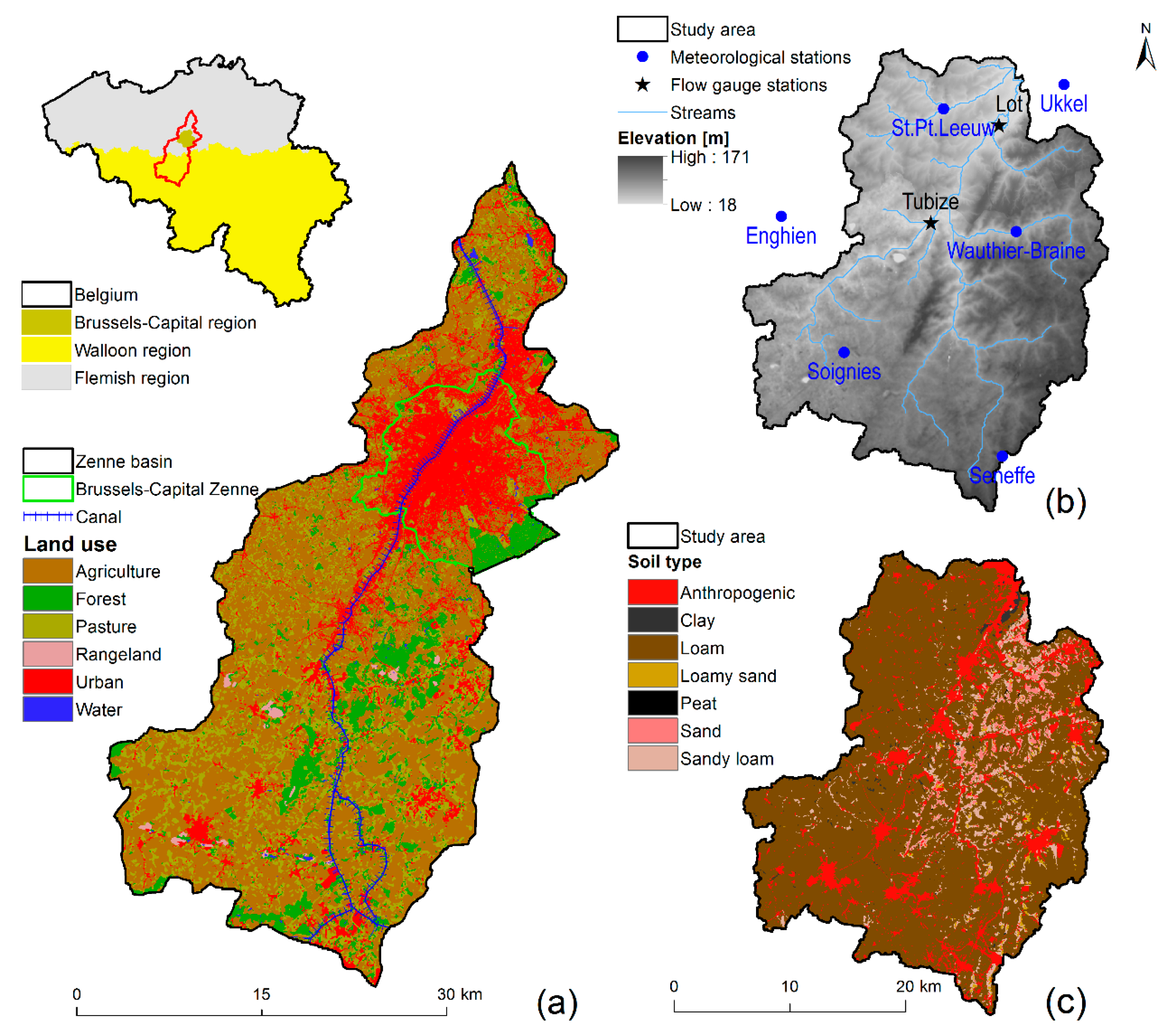
The Zenne river basin, which is part of the international Scheldt river basin, is situated in the central part of Belgium (Figure 1). The river drains a total area of 1162 km2 and crosses the three administrative regions of the country (Figure 1, top left corner). Zenne is the most populated and highly influenced (anthropogenic activity) basin in Belgium [51,52,53]. In addition, the basin is characterized by heterogeneous geological formations, groundwater recharge, and rainfall-runoff responses [48]. Because the basin is densely populated, the river receives high levels of organic pollutant and nutrient loadings [52,54]. Upstream from Brussels, the river experiences a natural meandering course, whereas it was vaulted over a distance of approximately 8 km in the Brussels region. To prevent the Brussels-Capital from flooding, the river is connected with a shipping canal, which is called the Brussels-Charleroi (upstream part) and the Sea Canal Brussels-Scheldt (downstream part) and runs parallel to the river (Figure 1a). The canal directly receives excess water from the main river reach during high flow conditions. In the Walloon region, the canal is fed by the complete diversion of the former tributaries of the river, such as Hain, Thines, and Samme [48,55]. Downstream from Brussels, the navigation canal discharges some of the received water back into the river [52]. Additionally, the Zenne river interacts with the densely networked sewer systems of Brussels [52,54]. In such conditions, extreme peak and low flows can play a significant role, given their considerable impact on river ecosystem, infrastructures, economy, and human life [7,24,26].
Due to intensive anthropogenic activities and urbanization in Brussels (Figure 1a), this study focused on the upstream part of the basin that ends at the Lot gauging station (Figure 1b). The area upstream of Lot covers an area of approximately 747 km2 and has a population density of 470 per km2 [48]. The upstream part of the basin is mainly covered with agriculture that accounts for 56% of the area, followed by pasture (22%), and mixed forest (11%). The rest of the area is covered with urban areas, rangeland, and water bodies (Figure 1a). Loam soils cover 79% of the upstream basin, with other soils (anthropogenic, sandy loam, sand, loamy sand, and clay) accounting for 21% of the basin (Figure 1c).
2.2. Data
The developed SWAT model utilized a 30 × 30 m Digital Elevation Model (DEM) obtained from the Flemish Land Council OC-GIS-Flanders (VLM-OC-GIS) and the Advanced Spaceborne Thermal Emission and Reflection Radiometer of Global DEM (ASTER GDEM), a 20 × 20 m soil map from OC-GIS-Flanders and the Digital Soil Map of Wallonia, and a 20 × 20 m land use map of 2000 from the OC-GIS-Flanders and the Ministry of Wallonia, Section Spatial Planning, Housing, and Heritage.
Daily precipitation data were obtained from the Royal Meteorological Institute (RMI) of Belgium at the Ukkel station for the period 1960 to 2008, from the Operational Section Mobility and Hydraulic Tracks (DGVH) at Enghien, Seneffe, Soignies and Wautier-Braine stations for the period 1990 to 2008, and from the Flemish Environmental Council (VMM) at the Saint-Pieters-Leeuw station for the period 1985 to 2001 (Figure 1b). Daily maximum and minimum temperatures, wind speed, solar radiation, and relative humidity were only available at the Ukkel station for the period 1960 to 2008. Additionally, while complete climatic data were available at Ukkel station, precipitation data at the other stations were incomplete and thus filled with the data from the Ukkel station. Furthermore, due to the similarity in observed rainfall magnitudes and strong correlations among the Ukkel and other stations, missing values were directly replaced with the values recorded at the Ukkel station. SWAT was calibrated and validated by using daily streamflow data of the period 1985 to 2008 measured at Tubize station of the DGVH and at Lot of the VMM (Figure 1b).
2.3. Streamflow Modeling
In order to assess the impact of future climate change on streamflow extreme values, we used the SWAT model, which was previously set up, calibrated, and validated by Leta et al. [48], for the upstream part of Zenne, ending at its outlet at the Lot station. Therefore, this study does not provide detailed model set-up, sensitivity analysis (SA), calibration, and validation processes, but briefly summarizes the methods used by Leta et al. [48]. The authors built the SWAT model using the geospatial and hydro-meteorological data mentioned in Section 2.2. In addition, the surface runoff was estimated using the modified Soil Conservation Service (SCS) Curve Number Method [56], whereas the Penman-Monteith [57] and Muskingum methods [58] were chosen for daily PET estimation and flow routing, respectively. Leta et al. [48] also implemented a simplified method in SWAT to consider the exchange of water between the river and canal at the upstream at Lembeek. Then, the authors applied detailed SA, which was based on the global Latin Hypercube One-factor-At-a-Time (LH-OAT) SA method [59], and identified the most sensitive and important parameters for the sub-sequent calibration and validation processes. Considering the high spatial heterogeneity of the basin, Leta et al. [48] applied three model calibration techniques. These were: (1) single-site calibration (SSC), which used only one flow gauging station at the basin outlet, i.e., Lot (Figure 1b); (2) sequential calibration (SC), which started calibration in the upstream station at Tubize (Figure 1b) and moved to the downstream part at Lot; and (3) simultaneous, multi-site calibration (SMSC), whereby data from both stations were simultaneously used in a single calibration. In the case of the SMSC method, the authors also used multi-objective functions. Leta et al. [48] found that of the three calibration techniques used, the SMSC provided the best results in terms of representing observed daily streamflow hydrographs and temporal variability, including reliable representation of water balance components of the basin. In addition, the authors documented that the SMSC technique allowed them to simultaneously calibrate the SWAT parameters that are structured at basin, sub-basin, and HRU spatial scales. The SMSC further helped to simultaneously communicate information contained in observed flow data at multiple stations, reduce model calibration bias, and easily capture the basin’s spatial variability. On the basis of their findings, this study also utilized the calibrated and validated SWAT model of the SMSC technique. The reader is referred to Leta et al. [48] and Leta [55] for the detailed approaches used for SWAT model inputs, set-up, SA, calibration, and validation procedures, including results, model performance evaluation criteria and prediction uncertainty.
2.4. Climate Change Scenarios
The CCI-HYDR perturbation tool [38,49,60] was used to obtain perturbed time series data of rainfall, minimum and maximum temperature to reflect future climate scenarios on the basis of the historical data of 1961–1990, which is hereafter called the control period. The perturbation tool was originally developed by the university of Leuven and the RMI of Belgium as part of the CCI-HYDR project, which refers to “Climate change impact on hydrological extremes in Belgium” for the Belgian Science Policy Office Program [49,61]. The tool is especially dedicated to the assessment of the hydrological impacts of climate change on rivers and urban drainage systems in Belgium. The CCI-HYDR tool was developed based on the four Special Report Emission Scenarios (SRES) (A1B, A2, B1 and B2) of the Intergovernmental Panel on Climate Change (IPCC) Fourth Assessment Report (AR4) [2]. The climate predictions for the A2 and B2 regional scenario families were extracted from the results and database of the regional climate models (RCMs) of the Prediction of Regional scenarios and Uncertainties for Defining EuropeaN Climate change risks and Effects (PRUDENCE) project [62,63]. However, the A1B and B1 scenarios were derived from the database and results of the GCMs of the IPCC-AR4 [64]. Hence, the scenarios in CCI-HYDR tool were derived from two databases in order to formulate an ensemble of different climate model outputs, such that they can reliably represent the possible range of climate change impacts in the future. The development of the CCI-HYDR tool primarily aimed to generate a few tailored climate change scenarios that could optimally represent the possible spectrum of all available climate change scenarios from various climate model runs, and thus allow an easy interpretation of the implications of future climate change in Belgium [38].
On the basis of the different climate model runs, the CCI-HYDR perturbation tool provides quantile perturbation factors for the variables precipitation, PET, and temperature. The factors are defined as the ratio between intensity value for the future defined time horizon (e.g., 2066–2095) and the corresponding value from the control period (1961–1990) for precipitation and PET [36,37,38]. In addition, for precipitation, the number of wet days and intensities are also taken into account [36,38]. Unlike precipitation and PET, the difference between the future and the control period was used for temperature projection. In addition, the use of quantile perturbation approach minimizes the bias in the climate model projections by calculating climate change signals from the climate model runs and applying these signals to observed climate data [38]. For the purpose of hydrological impact analysis, the perturbation factors (signals) of the CCI-HYDR tool were tailored into three scenarios [36,37,38]:
- High scenario: predicts the future climate with wet winters (high frontal rainfall) and wet summers (high convective storm rainfall)
- Mean scenario: projects a future with intermediate conditions
- Low scenario: considers dry (low rainfall) winters and dry summers in the future
The original CCI-HYDR tool only makes it possible to perturb the mean daily temperature. However, as the SWAT model requires both minimum and maximum temperature data, we used the modified version of the perturbation tool that perturbs both the minimum temperature (Tmin) and the maximum temperature (Tmax) [38,49]. The Tmin and Tmax perturbations and future predictions are based on the Long Ashton Research Station Weather Generator (LARS-WG) GCMs [65]. Note that the LARS-WG GCMs were included only for rescaling the Tmin and Tmax projections, and not for the other climatic variables. Hence, in addition to its original functionality, the modified CCI-HYDR tool perturbs the historical daily time series data of Tmin and Tmax [49]. Table 1 provides an overview of the four climate change scenarios that were formulated in the CCI-HYDR perturbation tool. Please note that the original high scenario of CCI-HYDR is split into a high (wet) summer and a high (wet) winter scenario.
The high, mean, and low refer to the expected hydrological impacts of climate change that are obtained based on climate change simulations and quantile perturbation (change) factors analysis [27,38]. From large sets of perturbation factors (derived from the different climate model runs), high, mean, and low perturbation factors are extracted. These factors are then applied to the observed rainfall, minimum and maximum temperature time series data in order to generate the corresponding perturbed input series for high, mean, and low scenarios. Approaches on high, mean, and low scenarios formulations and quantile perturbation factors estimation are detailed in Ntegeka et al. [38] and Van Uytven and Willems [49].
In this study, the climate change impact analysis also included the expected change in future solar radiation. In the absence of projected solar radiation data, we considered future solar radiation change based on previous studies. It has been reported that the solar radiation is anticipated to decrease by 5 to 15% during winter (December to February) and increase by 5 to 10% during summer (June to August) in most parts of Europe [50]. In addition, on the basis of 18 GCMs run for Europe, Ruosteenoja and Räisänen [50] also found that in autumn (September to November), the solar radiation patterns will qualitatively resemble that of summer, while the spring (March to May) solar radiation will likely be similar to that of the winter season. The authors projected solar radiation change for the period 2070 to 2099, under the A1B emission scenario. Based on their findings, we assumed the solar radiation will increase, on average, by 7.5% during the summer and autumn seasons, while a 10% decrease is considered for the spring and winter months, compared to the control values of 1961 to 1990.
Finally, for rainfall, minimum and maximum temperature changes, we used perturbed time series outputs of the CCI-HYDR tool as inputs to the SWAT model. However, for the solar radiation change, the control values were increased or decreased by multiplying by factors with a value of one meaning no change. For example, during summer and autumn seasons, a value of 1.075 was applied, indicating a 7.5% increase in solar radiation compared to the historical data. Similarly, a change value of 0.90 was used during the spring and winter seasons to reflect a 10% decrease in solar radiation values compared with the control values. The perturbation values for solar radiation change were implemented in the SWAT’s sub-basin files [66].
2.5. Extreme Peak and Low Flows Analysis
The calibrated and validated SWAT model of the Zenne river [48] was run with long-term control period (1961–1990) and future perturbed time series data. The simulated streamflow values for both the control and four future climate scenarios were post-processed to derive relative changes in extreme peak and low flows, including an ensemble range of relative changes and average values. For the extraction of daily extreme peak and low flow values from simulated daily streamflows, we used the Water Engineering Time Series PROcessing (WETSPRO) tool developed by Willems [67]. The tool selects the extreme peak flow values from daily time series data based on the independent peak over threshold (POT) method as described in Willems [67]. WETSPRO extracts two subsequent peak flows from the flow series when the following three criteria are simultaneously fulfilled [28,67].
- (1)
- The time length of the decreasing flank of the first peak flow event is greater than a minimum threshold time, which can be assigned to the recession constant of the quick flow or larger value;
- (2)
- The flow in between the two peak events should drop down to a fraction lower than a given threshold fraction value of the peak flow;
- (3)
- The flow increment between the peak flow and lowest flow (in between the current and previous peak flows) should have a minimum height. This criterion is considered to avoid the selection of a small noise peaks.
In such analysis, the SWAT simulated daily streamflows for both the control and future periods were used as inputs to WETSPRO. Similarly, the WETSPRO tool was used to estimate the low flow values, which were selected on the basis of the lowest annual flow value [67]. For the low flows selection, the WETSPRO still uses the POT approach, but transforms the original daily streamflow values into their corresponding reciprocal values. Such transformation converts the minimum flow to maximum flow and thus facilitates the easy extraction of extreme low flow values [11]. However, we eventually transformed back the WETSPRO selected extreme low flows to their original values only for the purpose of plotting, graphical analysis, and easy interpretation. Lastly, for both the selected extreme peak and low flow values, we ranked them from high to low and low to high, respectively, and calculated the corresponding return periods as
where is the return period [year] of the peak or low flow values, and are rank and the total number of years of simulation period, respectively. Relative changes in extreme peak and low flow values were plotted against the estimated return periods. Detailed approaches on extreme peak and low flows selection are described in Willems [67].
3. Results and Discussion
3.1. Projected Climate Variables
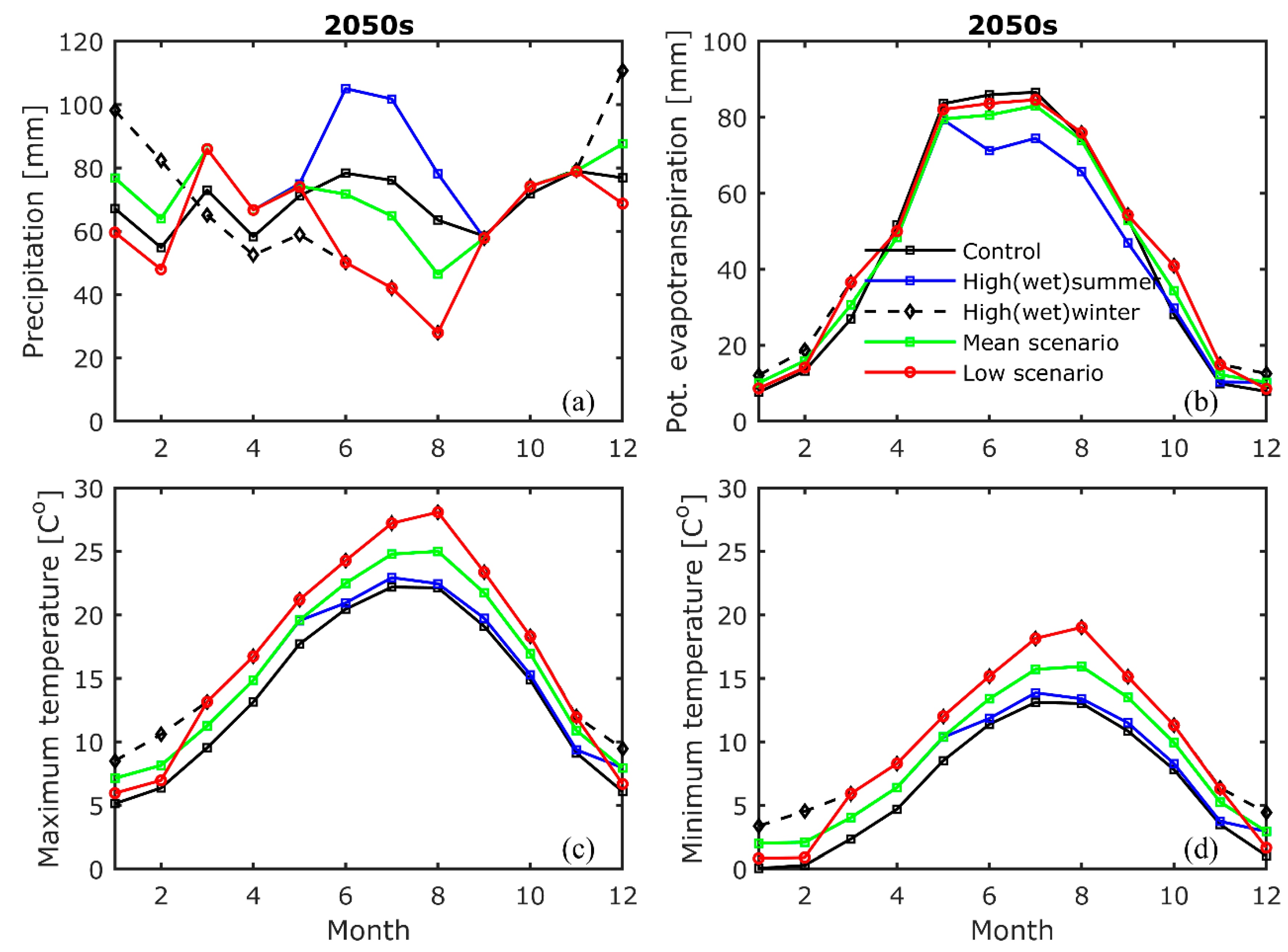
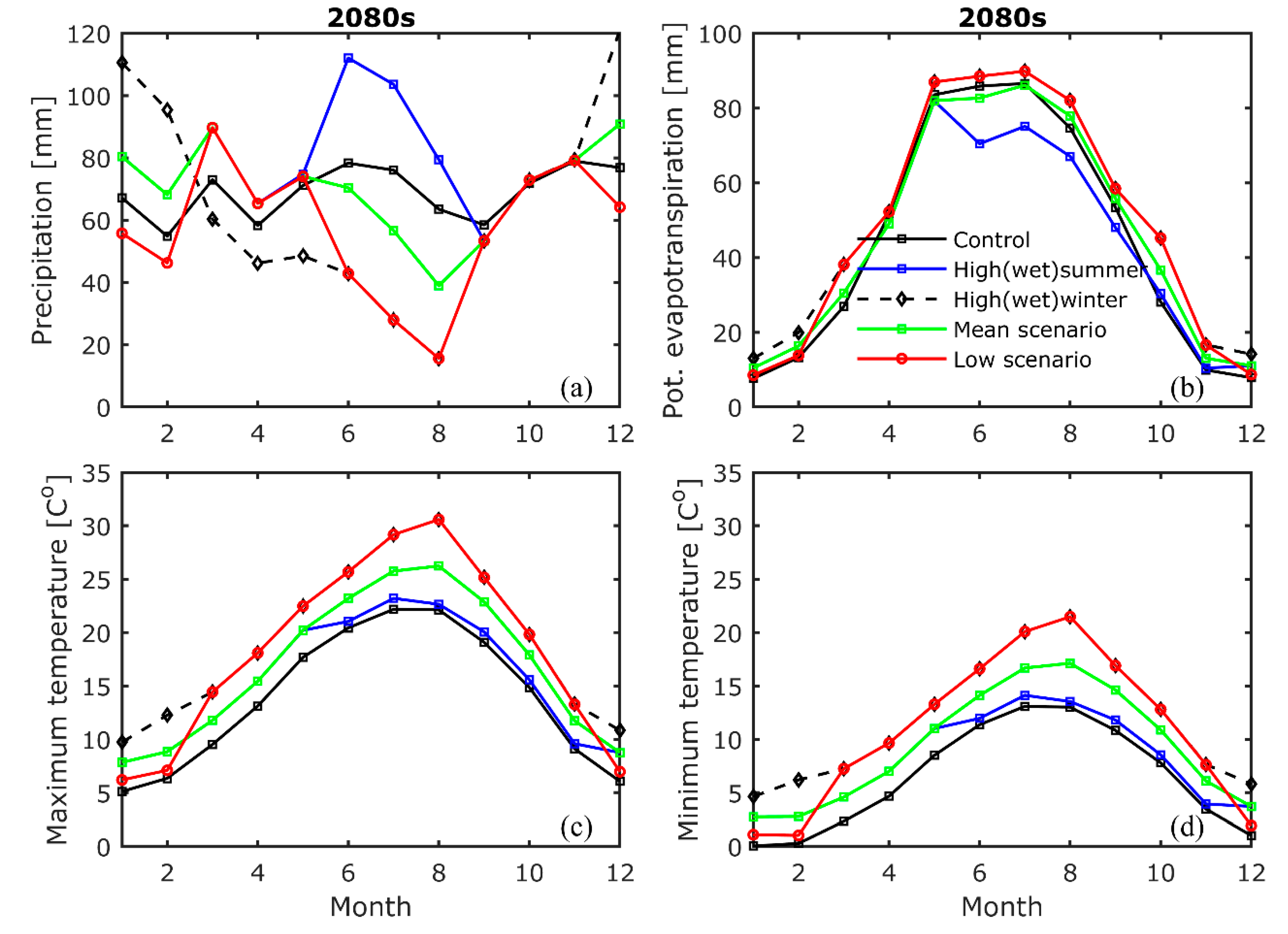
The average monthly outputs of the CCI-HYDR tool for the four climate change scenarios listed in Table 1, along with the control period, are shown in Figure 2 and Figure 3 for both the 2050s and 2080s. The figures indicate that the minimum and maximum temperatures will generally increase by the middle and end of this century. The summer precipitation is expected to decrease for all the scenarios, except the high (wet) summer scenario (Figure 2 and Figure 3). PET will slightly increase for most of the scenarios, but a decrease is notably predicted during the summer months of the high (wet) summer scenario. The latter should be expected due to minimal increase in temperature and considerable increase in precipitation during the summer season (Figure 2 and Figure 3).
In general, it is noted that the general variations and trends are similar for both the 2050s and 2080s scenarios. However, the change of the variables in the 2080s will be more pronounced. For example, for the low (dry) scenario, the monthly average precipitation is expected to decrease by 11% and 17% by the 2050s and the 2080s, respectively. In addition, under the same scenario, the summer precipitation and temperature are expected to face the largest negative and positive changes, respectively, when compared to the control values (Figure 2 and Figure 3). In contrast to the low (dry) scenario, the high (wet) summer scenario is expected to cause significant increase in summer rainfall that may cause a potential decrease in PET compared to the control values and the other scenarios (Figure 2 and Figure 3).
3.2. Impact of Climate Change on Extreme Peak Flows
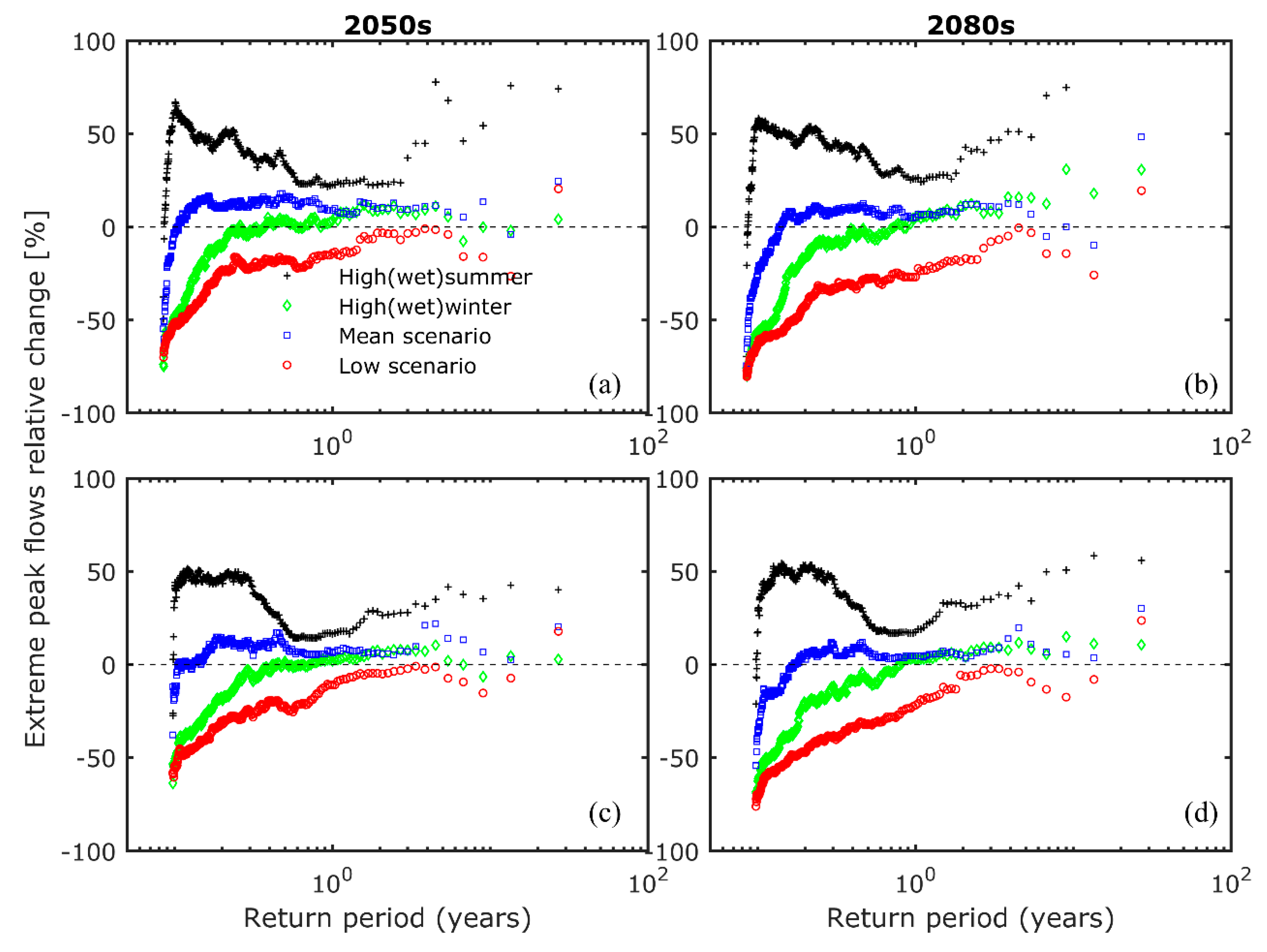
The relative sensitivity of extreme peak flows to the four climate change scenarios is summarized in Table 2. The table also lists the ensemble range of relative changes based on the four climate change scenarios and the corresponding average values. The ensemble range and their average values were computed based on the four climate change scenarios listed in Table 1. Table 2 shows a wide range of the impact of the different scenarios on extreme peak flow values. The relative changes in peak flows are positive or negative depending on the applied scenarios. For example, the extreme peak flow change is in the range of −80 to 109% for Tubize and −76 to 58% for Lot. While the direction of change in peak flows for individual scenarios is inconclusive, the table, however, indicates an overall decrease in peak flows under all scenarios (ensemble average values) in comparison to the control values. More importantly, we clearly observed that the impact of climate change on extreme peak flows is much higher under the low (dry) and high (wet) summer scenarios (Table 2 and Figure 4), which is most likely due to increase in precipitation, temperature, and solar radiation during the summer season.
Under the high (wet) summer scenario, an overall increase of 43% in peak flows is expected (Figure 4 and Figure 5). However, a larger positive change is projected for flows with higher return periods of approximately 4 years (Figure 5), which implies that the control period distributions are considerably shifted upwards, and higher peak flows are predicted under the same return periods of the control values. This is most probably due to a significant increase in precipitation and decrease in PET during the summer season (see Figure 2 and Figure 3). In such circumstances, the soils are expected to be at saturated condition (lower infiltration values) and thus likely generate more surface runoff and peak flows when compared to control values. Such events can potentially cause frequent occurrence of flooding and may have adverse consequences, such as damage to infrastructures or drainage systems and negatively impact the downstream Brussels, as well as its population. The high (wet) summer scenario is also expected to increase the frequency of overflows to the Brussels-Charleroi canal that would in turn cause shipping traffic and more sedimentation in the canal. In contrast to this scenario, the peak flows under the low (dry) scenario are generally expected to decrease (Table 2 and Figure 5). However, larger negative change is projected for peak flows with return periods of smaller than about two years. This could be expected due to higher negative changes in precipitation especially during the dry season (Figure 2 and Figure 3). In such conditions, the soil surface will probably be less saturated, due to limited moisture availability, and will thus cause a larger rainfall initial abstraction (higher infiltration values). This may result in smaller peak flow values when compared to the control values. The high (wet) winter and mean scenarios are expected to cause impacts (relative changes) that are generally between the high (wet) summer and low (dry) scenarios (Table 2 and Figure 5), which is also consistent with previous studies in Belgium regarding the impact of climate change [27,28,46].
Additionally, as can be clearly noted in Table 2 and Figure 5, while the directions of relative change in extreme peak flows are similar for the upstream and downstream stations of the basin, the impact is relatively more important for the south-western part of the basin than the downstream. For example, both larger negative and positive changes in extreme peak flows are predicted at Tubize in comparison to the Lot station (Table 2 and Figure 5), indicating the high spatial variability of the basin’s response to climate change and thus reflecting the influence of the basin’s characteristics on the impact of climate change. This could be partly related to a larger contribution of surface runoff to streamflow in the south-western part of the basin and to the overflow to the canal at Lembeek, which is well documented by Leta et al. [48] and Leta [55]. These authors also reported that the south-western part of Zenne acts as a discharge zone (recharge close to zero), compared to the rest part of the basin, due to geological heterogeneity, difference in rainfall-runoff responses, and basin parameters. Our findings imply that the difference in basin characteristics may play a significant role in the impact of climate change on extreme peak flows, and thus provide different degrees of response (sensitivity) to climate change.
Overall, the wider range in relative change of peak flows of −80 to 109% indicates the high uncertainty in predicting future climate change impact on extreme peak flows. However, these relative changes may include different uncertainties originating from model parameters, model structure, and inputs. Leta et al. [68] and Leta [55] reported that the total model prediction uncertainty at Tubize, including rainfall uncertainty, is between −75 to 92%, with an average value of ±17%. Note that the authors estimated the total uncertainty range from the lower (2.5%) and upper (97.5%) bands with respect to the observed daily flows (see Leta et al. [68] and Leta [55] for detail). When the total model prediction uncertainty range is compared with the range of relative changes in extreme peak flows due to the four climate change scenarios, the climate change uncertainty still shows a significant impact than model prediction uncertainty, due to its wider band. This stresses that serious mitigation measures for future climate change should be adopted, if these scenarios should take place. In general, our findings are in line with previous studies regarding climate change impacts on basins in Belgium [27,28,45].
3.3. Impact of Climate Change on Extreme Low Flows
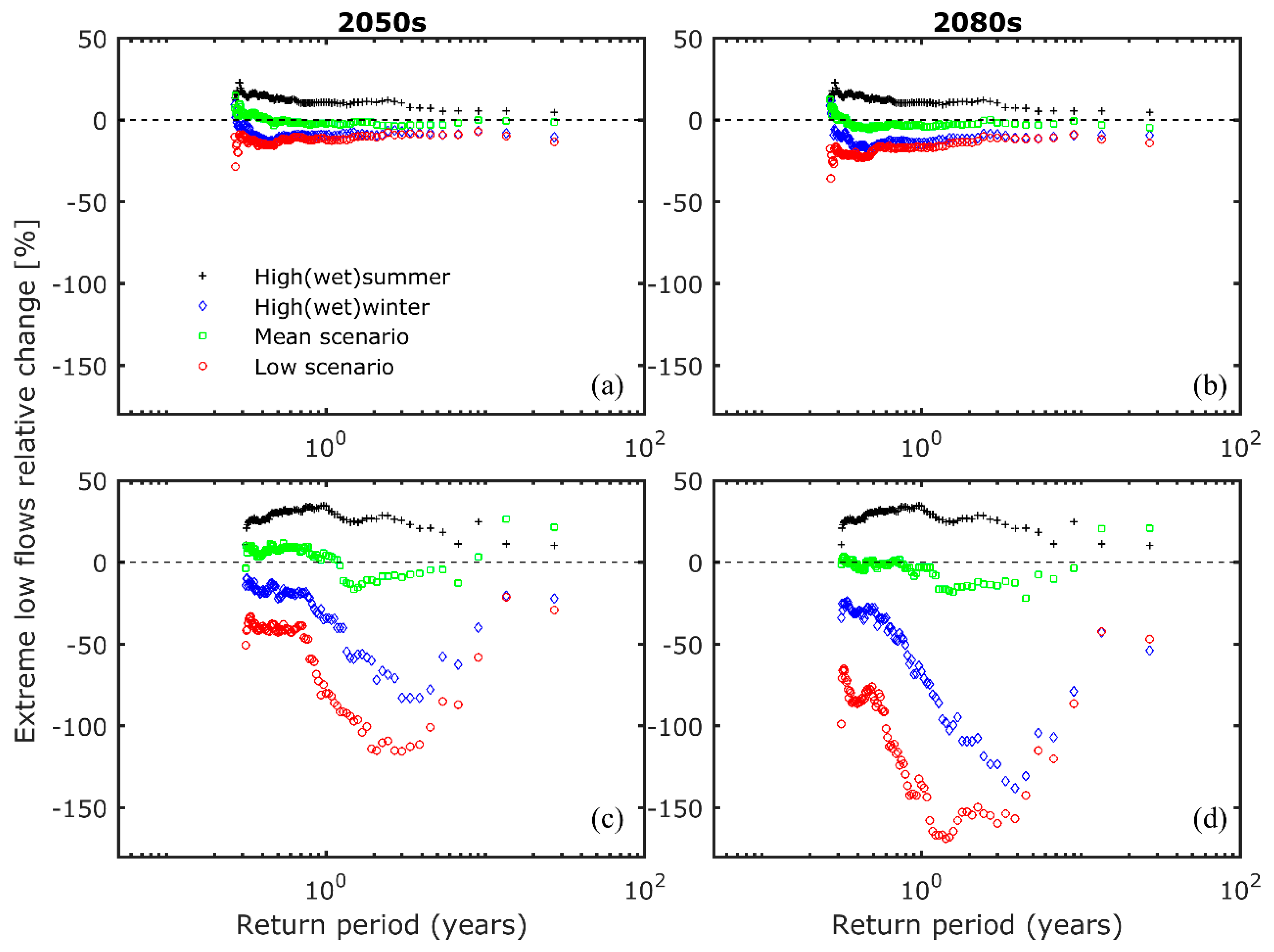
For the low flows, the low (dry) and high (wet) winter scenarios generally point towards drier conditions (Table 3, Figure 6 and Figure 7), which is consistent with the rainfall and temperature changes listed in Table 1. A consistent decrease in low flows under these scenarios are probably due to less rainfall and high PET, particularly during the summer months (Figure 2 and Figure 3). However, the high (wet) summer scenario is projected to cause a consistent increase in low flows (Table 3 and Figure 7), which is likely to be due to an overall increase in rainfall and decrease in PET especially during the summer season. The table and figure also reveal that larger negative changes in low flows are anticipated under the low (dry) scenario followed by the high (wet) winter scenario. This should be expected, as the precipitation is projected to decrease, while PET is expected to increase in the summer season when groundwater flow contribution to low flows is high. Thus, the low (dry) and high (wet) winter scenarios are expected to cause considerable downward shifts in low flow distributions and more frequent occurrence of smaller low flow values under the same return periods of the control values. This implies that periods of hydrological drought are expected to be more frequent if low (dry) and high (wet) winter scenarios should occur. This will likely cause earlier occurrence of hydrological droughts compared to the hydrological regime of the control period. This is expected to be amplified towards the end of this century (Table 3 and Figure 7).
Overall, the low flows are generally predicted to decrease except under the high (wet) summer scenario. Such changes may have potential implications on the major agricultural crop productivity and the minimal ecological flow requirement of the basin. In addition, as the river, as well as the upstream sub-basins of south-eastern part [48,55], feed the canal, the water may be too low to meet the required amount of water for the connected canal. In that case, various sectors may be affected, such as navigation and recreation activities. The mean scenario is anticipated to be similar to the control period, and is thus expected to have a minor impact on low flows or for them to remain in a stable condition (Figure 6 and Figure 7). As opposed to peak flows, both larger negative and positive relative changes in low flows are projected to occur in the downstream part of the basin, where a higher groundwater contribution is expected [48,55]. For example, the relative change in low flows is predicted to be between −36 to 23% at Tubize and −169 to 34 at Lot (Table 3) by 2080s.
While the relative changes in low flows are consistent with previous studies [28,69], the results should be interpreted with caution. Although groundwater flow is the main source of the low flows during the dry seasons, SWAT uses a simplified linear reservoir module for the representation of the groundwater system. Hence, the approach used in SWAT might not well represent the physical basis of groundwater and its interactions with river. In such cases, the recession constant parameter used by SWAT may provide an average value and be too sensitive to climate change. In addition, previous studies on the low flows simulated by different basin models showed that the model structural uncertainties are very high during dry seasons, and thus the degree of model sensitivity to climate change (relative change) may be quite different even for the same climate change inputs, due to an oversimplified representation of groundwater system [28,40]. For instance, Vansteenkiste et al. [28] compared the climate change impact on low flows using the detailed MIKE-SHE and the simplified WetSpa models for groundwater modeling, and found that although the two models showed the same directions of climate change impact, the degrees of impact on the low flows were considerably different. This indicates that water resources managers and decision-makers should be aware of the role of hydrological model uncertainty in predicting future climate change impacts, suggesting the need to take into account those uncertainties in their decision-making process when they design and implement mitigation measures for climate change.
Finally, the significant impact of evapotranspiration on low flows is clearly observed based on the larger percent of negative changes (Table 3 and Figure 7). This is probably due to the high sensitivity of low flows to precipitation, temperature, and solar radiation changes during the summer season. This is more pronounced for flows with higher return periods. In general, while the 2050s and the 2080s scenarios show similar trends in change for low flows, the 2080s scenario is predicted to cause a higher magnitude of the change compared to the 2050s change. For example, under the low scenario, low flows at Lot are predicted to decrease by as much as 83% and 169% by 2050s and 2080s, respectively.
4. Summary and Conclusions
In this study, we utilized the previously developed, calibrated, and validated SWAT model by Leta et al. [48] for the upstream part of Zenne basin (Belgium). This study aimed to use the model for assessing the impact of climate change on daily hydrological extreme values (peak and low flows). In order to provide an overall detailed basin-wide assessment of the impact of climate change on the basin, we generated four climate change scenarios (high (wet) summer, high (wet) winter, mean, and low (dry)) using the CCI-HYDR tool [38,49], which was primarily developed to assess the impact of climate change on hydrological extremes of Belgian basins. The tool was used to generate perturbed time series data of precipitation, minimum and maximum temperature for the period 2036–2065 (2050s) and the 2065–2095 (2080s). Seasonal solar radiation change was also considered based on previous studies [50]. For both of the 2050s and 2080s time horizons, perturbed future time series data were prepared for a period of 30 years, based on the historical time series of 1961–1990. Daily extreme peak flows (floods) and low flows (droughts) were extracted for both the control period and four future climate change scenarios for the 2050s and 2080s by using the WETSPRO tool [67].
This study provided a quantitative analysis of the impact of climate change on peak and low flows through estimating possible range of relative changes under four climate change scenarios for a case study in Belgium. We found that the daily peak flows are expected to increase by as much as 109% under the high (wet) summer scenario. This scenario thus points to an increased risk of adverse effects, such as frequent flooding, damage of infrastructures and drainage systems in the downstream Brussels-Capital, disturbance of the riverine ecosystem, and loss of inhabitants along the river. On the other hand, the low (dry) scenario is expected to cause a consistent decrease in both daily peak and low flows, due to an overall decline in rainfall, increase in temperature, solar radiation, and thus evapotranspiration. Under this scenario, low flows are projected to consistently decrease by as much as 169% compared to the control values. More importantly, earlier occurrence of hydrological droughts is expected when compared to the hydrological regime of the control period, which is anticipated to be amplified towards the end of the 21st century. Thus, the dry scenario would cause severe problems, such as droughts, reduction in agricultural crop productivity, and decrease in water supply to water harvesting structures, such as the shipping canal, and increase in other water use demands. While larger positive changes in peak flows are predicted for the upstream part of the basin, larger negative changes in low flows are projected for the downstream part, where a higher groundwater contribution is expected. Such changes indicate that basin characteristics may play a significant role in the impact of climate change and thus on the degree of sensitivity of a basin to climate change, suggesting the importance of spatially assessing the impact of climate change on hydrological extremes, in contrast to the tradition approach that focused at basin outlet. This is critically important for basins that experience high spatial heterogeneity, like the Zenne basin. The study also found that the relative impact of climate change is higher for low flows than for high flows, indicating an overall drier condition in the future. However, the results for the low flows should be considered with caution as they might be influenced by the model structure of SWAT because the model uses a simplified linear reservoir equation for groundwater system representation.
In general, the findings indicate that the four climate change scenarios show quite different impacts on the daily extreme peak and low flows. We found that the projected changes strongly depend on the applied climate change scenarios and the direction of change is highly uncertain, which is also consistent with previous studies in Belgium [27,28,45]. However, our ensemble average values indicate that an overall decline in extreme peak and low flows is expected. The low flows are generally predicted to show significant downward trends compared to peak flows. Due to such severe consequences of climate change, water resource managers and ecosystem conservationists need to design and implement appropriate mitigation measures for climate change. In addition, they should be aware of hydrological model prediction uncertainty, such as described in the work of Leta et al. [68], which needs to be accounted for in their decision-making process.
Author Contributions
O.T.L. conceived, performed the simulations, analyzed the data and results, and wrote the paper. W.B. supervised the research, contributed to results interpretation, and edited the paper.
Funding
This research was funded through the Environmental Impulse Program (INNOVIRIS) of the Brussels-Capital Region.
Acknowledgments
The authors would like to thank all the institutions and administrations mentioned in this paper for providing the required data. The authors are also indebted to Victor Ntegeka for modifying the original CCI-HYDR perturbation tool in order to generate perturbed future minimum and maximum temperature data.
Conflicts of Interest
The authors declare no conflicts of interest.
References
- Ahmed, K.F.; Wang, G.; Silander, J.; Wilson, A.M.; Allen, J.M.; Horton, R.; Anyah, R. Statistical downscaling and bias correction of climate model outputs for climate change impact assessment in the U.S. northeast. Glob. Planet. Chang. 2013, 100, 320–332. [Google Scholar] [CrossRef]
- IPCC. Climate Change 2007: The Physical Science Basis. Contribution of Working Group I to the Fourth Assessment; Cambridge University Press: Cambridge, UK; New York, NY, USA, 2007; p. 996. ISBN 978-0521-70596-7. [Google Scholar]
- IPCC. Climate Change 2007: Impacts, Adaptation and Vulnerability. Contribution of Working Group II to the Fourth Assessment; Cambridge University Press: Cambridge, UK; New York, NY, USA, 2007; p. 976. ISBN 978-0521-70597-4. [Google Scholar]
- Leta, O.T.; El-Kadi, A.I.; Dulai, H.; Ghazal, K.A. Assessment of climate change impacts on water balance components of Heeia watershed in Hawaii. J. Hydrol. Reg. Stud. 2016, 8, 182–197. [Google Scholar] [CrossRef]
- Leta, O.T.; El-Kadi, A.I.; Dulai, H. Implications of climate change on water budgets and reservoir water harvesting of Nuuanu area watersheds, Oahu, Hawaii. J. Water Resour. Plan. Manag. 2017, 143, 05017013. [Google Scholar] [CrossRef]
- Shrestha, N.K.; Du, X.; Wang, J. Assessing climate change impacts on fresh water resources of the Athabasca River Basin, Canada. Sci. Total Environ. 2017, 601, 425–440. [Google Scholar] [CrossRef] [PubMed]
- Mohammed, K.; Islam, A.K.M.S.; Islam, G.M.T.; Alfieri, L.; Bala, S.K.; Khan, M.J.U. Impact of High-End Climate Change on Floods and Low Flows of the Brahmaputra River. J. Hydrol. Eng. 2017, 22, 04017041. [Google Scholar] [CrossRef]
- Bodian, A.; Dezetter, A.; Diop, L.; Deme, A.; Djaman, K.; Diop, A. Future Climate Change Impacts on Streamflows of Two Main West Africa River Basins: Senegal and Gambia. Hydrology 2018, 5, 21. [Google Scholar] [CrossRef]
- Ahiablame, L.; Sinha, T.; Paul, M.; Ji, J.-H.; Rajib, A. Streamflow response to potential land use and climate changes in the James River watershed, Upper Midwest United States. J. Hydrol. Reg. Stud. 2017, 14, 150–166. [Google Scholar] [CrossRef]
- Vetter, T.; Reinhardt, J.; Flörke, M.; van Griensven, A.; Hattermann, F.; Huang, S.; Koch, H.; Pechlivanidis, I.G.; Plötner, S.; Seidou, O.; et al. Evaluation of sources of uncertainty in projected hydrological changes under climate change in 12 large-scale river basins. Clim. Chang. 2017, 141, 419–433. [Google Scholar] [CrossRef]
- Taye, M.T.; Ntegeka, V.; Ogiramoi, N.P.; Willems, P. Assessment of climate change impact on hydrological extremes in two source regions of the Nile River Basin. Hydrol. Earth Syst. Sci. 2011, 15, 209–222. [Google Scholar] [CrossRef] [Green Version]
- Leta, O.T.; El-Kadi, A.I.; Dulai, H. Impact of Climate Change on Daily Streamflow and Its Extreme Values in Pacific Island Watersheds. Sustainability 2018, 10, 2057. [Google Scholar] [CrossRef]
- Mantua, N.; Tohver, I.; Hamlet, A. Climate change impacts on streamflow extremes and summertime stream temperature and their possible consequences for freshwater salmon habitat in Washington State. Clim. Chang. 2010, 102, 187–223. [Google Scholar] [CrossRef]
- Beniston, M.; Stephenson, D.; Christensen, O.; Ferro, C.; Frei, C.; Goyette, S.; Halsnaes, K.; Holt, T.; Jylhä, K.; Koffi, B.; et al. Future extreme events in European climate: An exploration of regional climate model projections. Clim. Chang. 2007, 81, 71–95. [Google Scholar] [CrossRef]
- Blenkinsop, S.; Fowler, H.J. Changes in European drought characteristics projected by the PRUDENCE regional climate models. Int. J. Climatol. 2007, 27, 1595–1610. [Google Scholar] [CrossRef] [Green Version]
- De Wit, M.J.M.; Hurk, B.; Warmerdam, P.M.M.; Torfs, P.J.J.F.; Roulin, E.; Deursen, W.P.A. Impact of climate change on low-flows in the river Meuse. Clim. Chang. 2007, 82, 351–372. [Google Scholar] [CrossRef] [Green Version]
- Feyen, L.; Dankers, R. Impact of global warming on streamflow drought in Europe. J. Geophys. Res. 2009, 114, D17116. [Google Scholar] [CrossRef]
- Jiang, T.; Chen, Y.D.; Xu, C.-Y.; Chen, X.; Chen, X.; Singh, V.P. Comparison of hydrological impacts of climate change simulated by six hydrological models in the Dongjiang Basin, South China. J. Hydrol. 2007, 336, 316–333. [Google Scholar] [CrossRef]
- Firing, Y.L.; Merrifield, M.A. Extreme sea level events at Hawaii: Influence of mesoscale eddies. Geophys. Res. Lett. 2004, 31, L24306. [Google Scholar] [CrossRef]
- Firing, Y.L.; Merrifield, M.A.; Schroeder, T.A.; Qiu, B. Interdecadal Sea Level Fluctuations at Hawaii. J. Phys. Oceanogr. 2004, 34, 2514–2524. [Google Scholar] [CrossRef]
- Caccamise, D.J.; Merrifield, M.A.; Bevis, M.; Foster, J.; Firing, Y.L.; Schenewerk, M.S.; Taylor, F.W.; Thomas, D.A. Sea level rise at Honolulu and Hilo, Hawaii: GPS estimates of differential land motion. Geophys. Res. Lett. 2005, 32, L03607. [Google Scholar] [CrossRef]
- Storlazzi, C.D.; Elias, E.P.L.; Berkowitz, P. Many Atolls May be Uninhabitable Within Decades Due to Climate Change. Sci. Rep. 2015, 5, 14546. [Google Scholar] [CrossRef] [PubMed] [Green Version]
- Storlazzi, C.D.; Gingerich, S.B.; van Dongeren, A.; Cheriton, O.M.; Swarzenski, P.W.; Quataert, E.; Voss, C.I.; Field, D.W.; Annamalai, H.; Piniak, G.A.; et al. Most atolls will be uninhabitable by the mid-21st century because of sea-level rise exacerbating wave-driven flooding. Sci. Adv. 2018, 4. [Google Scholar] [CrossRef] [PubMed]
- Habel, S.; Fletcher, C.H.; Rotzoll, K.; El-Kadi, A.I. Development of a model to simulate groundwater inundation induced by sea-level rise and high tides in Honolulu, Hawaii. Water Res. 2017, 114, 122–134. [Google Scholar] [CrossRef] [PubMed]
- Rotzoll, K.; Fletcher, C.H. Assessment of groundwater inundation as a consequence of sea-level rise. Nat. Clim. Chang. 2012, 3, 477–481. [Google Scholar] [CrossRef]
- Porter, K.; Wein, A.; Alpers, C.; Baez, A.; Barnard, P.; Carter, J.; Corsi, A.; Costner, J.; Cox, D.; Das, T.; et al. Overview of the ARkStorm Scenario; Open File Report 2010-1312; U.S. Geological Survey: Reston, VA, USA, 2011; p. 183.
- Poelmans, L.; Van Rompaey, A.; Ntegeka, V.; Willems, P. The relative impact of climate change and urban expansion on peak flows: A case study in central Belgium. Hydrol. Process. 2011, 25, 2846–2858. [Google Scholar] [CrossRef]
- Vansteenkiste, T. Climate change impact on river flows and catchment hydrology: A comparison of two spatially distributed models. Hydrol. Process. 2013, 27, 3649–3662. [Google Scholar] [CrossRef]
- Arnold, J.G.; Srinivasan, R.; Muttiah, R.S.; Williams, J.R. Large area hydrologic modeling and assessment Part I: Model development. JAWRA J. Am. Water Resour. Assoc. 1998, 34, 73–89. [Google Scholar] [CrossRef]
- Elsner, M.; Cuo, L.; Voisin, N.; Deems, J.; Hamlet, A.; Vano, J.; Mickelson, K.B.; Lee, S.-Y.; Lettenmaier, D. Implications of 21st century climate change for the hydrology of Washington State. Clim. Chang. 2010, 102, 225–260. [Google Scholar] [CrossRef] [Green Version]
- Jennings, E.; Allott, N.; Pierson, D.C.; Schneiderman, E.M.; Lenihan, D.; Samuelsson, P.; Taylor, D. Impacts of climate change on phosphorus loading from a grassland catchment: Implications for future management. Water Res. 2009, 43, 4316–4326. [Google Scholar] [CrossRef] [PubMed]
- Prudhomme, C.; Reynard, N.; Crooks, S. Downscaling of global climate models for flood frequency analysis: Where are we now? Hydrol. Process. 2002, 16, 1137–1150. [Google Scholar] [CrossRef]
- Willems, P.; Vrac, M. Statistical precipitation downscaling for small-scale hydrological impact investigations of climate change. J. Hydrol. 2011, 402, 193–205. [Google Scholar] [CrossRef]
- Willems, P.; Arnbjerg-Nielsen, K.; Olsson, J.; Nguyen, V.T.V. Climate change impact assessment on urban rainfall extremes and urban drainage: Methods and shortcomings. Atmos. Res. 2012, 103, 106–118. [Google Scholar] [CrossRef]
- Taye, M.T.; Willems, P. Influence of downscaling methods in projecting climate change impact on hydrological extremes of upper Blue Nile basin. Hydrol. Earth Syst. Sci. Discuss. 2013, 10, 7857–7896. [Google Scholar] [CrossRef] [Green Version]
- Ntegeka, V.; Baguis, P.; Boukhris, O.; Willems, P.; Roulin, E. Climate Change Impact on Hydrological Extremes along Rivers and Urban Drainage Systems. II. Study of Rainfall and ETo Climate Change Scenarios; Technical Report CCI-HYDR Project; Belgian Science Policy—SSD Research Programme; KU Leuven—Hydraulics Section & Royal Meteorological Institute of Belgium: Leuven, Belgium, 2008; p. 112. [Google Scholar]
- Baguis, P.; Ntegeka, V.; Willems, P.; Roulin, E. Extension of CCI-HYDR Climate Change Scenarios for INBO; Technical Report; Instituut voor Natuur-en Bosonderzoek (INBO) & Belgian Science Policy—SSD Research Programme; KU Leuven—Hydraulics Section & Royal Meteorological Institute of Belgium: Brussels, Belgium, 2009; p. 31. [Google Scholar]
- Ntegeka, V.; Baguis, P.; Roulin, E.; Willems, P. Developing tailored climate change scenarios for hydrological impact assessments. J. Hydrol. 2014, 508, 307–321. [Google Scholar] [CrossRef]
- Faramarzi, M.; Abbaspour, K.C.; Ashraf Vaghefi, S.; Farzaneh, M.R.; Zehnder, A.J.B.; Srinivasan, R.; Yang, H. Modeling impacts of climate change on freshwater availability in Africa. J. Hydrol. 2013, 480, 85–101. [Google Scholar] [CrossRef]
- Bae, D.-H.; Jung, I.-W.; Lettenmaier, D.P. Hydrologic uncertainties in climate change from IPCC AR4 GCM simulations of the Chungju Basin, Korea. J. Hydrol. 2011, 401, 90–105. [Google Scholar] [CrossRef]
- Githui, F.; Gitau, W.; Mutua, F.; Bauwens, W. Climate change impact on SWAT simulated streamflow in western Kenya. Int. J. Climatol. 2009, 29, 1823–1834. [Google Scholar] [CrossRef] [Green Version]
- Devkota, L.P.; Gyawali, D.R. Impacts of climate change on hydrological regime and water resources management of the Koshi River Basin, Nepal. J. Hydrol. Reg. Stud. 2015, 4, 502–515. [Google Scholar] [CrossRef]
- Rahman, K.; Etienne, C.; Gago-Silva, A.; Maringanti, C.; Beniston, M.; Lehmann, A. Streamflow response to regional climate model output in the mountainous watershed: A case study from the Swiss Alps. Environ. Earth Sci. 2014, 72, 4357–4369. [Google Scholar] [CrossRef]
- Ntegeka, V.; Willems, P. Trends and multidecadal oscillations in rainfall extremes, based on a more than 100-year time series of 10 min rainfall intensities at Uccle, Belgium. Water Resour. Res. 2008, 44. [Google Scholar] [CrossRef] [Green Version]
- Bauwens, A.; Sohier, C.; Degré, A. Hydrological response to climate change in the Lesse and the Vesdre catchments: Contribution of a physically based model (Wallonia, Belgium). Hydrol. Earth Syst. Sci. 2011, 15, 1745–1756. [Google Scholar] [CrossRef]
- Baguis, P.; Roulin, E.; Willems, P.; Ntegeka, V. Climate change and hydrological extremes in Belgian catchments. Hydrol. Earth Syst. Sci. Discuss. 2010, 7, 5033–5078. [Google Scholar] [CrossRef] [Green Version]
- Dams, J.; Salvadore, E.; Van Daele, T.; Ntegeka, V.; Willems, P.; Batelaan, O. Spatio-temporal impact of climate change on the groundwater system. Hydrol. Earth Syst. Sci. 2012, 16, 1517–1531. [Google Scholar] [CrossRef] [Green Version]
- Leta, O.T.; van Griensven, A.; Bauwens, W. Effect of Single and Multisite Calibration Techniques on the Parameter Estimation, Performance, and Output of a SWAT Model of a Spatially Heterogeneous Catchment. J. Hydrol. Eng. 2017, 22, 05016036. [Google Scholar] [CrossRef]
- Van Uytven, E.; Willems, P. Climate Perturbation Tool: Manual; KU Leuven: Leuven, Belgium, 2015; p. 20. [Google Scholar]
- Ruosteenoja, K.; Räisänen, P. Seasonal changes in solar radiation and relative humidity in Europe in response to global warming. J. Clim. 2013, 26, 2467–2481. [Google Scholar] [CrossRef]
- Chen, W.Y.; Liekens, I.; Broekx, S. Identifying Societal Preferences for River Restoration in a Densely Populated Urban Environment: Evidence from a Discrete Choice Experiment in Central Brussels. Environ. Manag. 2017, 60, 263–279. [Google Scholar] [CrossRef] [PubMed]
- Shrestha, N.K.; Leta, O.T.; Bauwens, W. Development of RWQM1-based Integrated water quality model in OpenMI with application to the River Zenne, Belgium. Hydrol. Sci. J. 2017, 62, 774–799. [Google Scholar] [CrossRef]
- Leta, O.; Shrestha, N.; de Fraine, B.; van Griensven, A.; Bauwens, W. Integrated Water Quality Modelling of the River Zenne (Belgium) Using OpenMI. In Advances in Hydroinformatics; Gourbesville, P., Cunge, J., Caignaert, G., Eds.; Springer: Singapore, 2014; pp. 259–274. [Google Scholar]
- Shrestha, N.K.; Leta, O.T.; de Fraine, B.; Garcia-Armisen, T.; Ouattara, N.K.; Servais, P.; van Griensven, A.; Bauwens, W. Modelling Escherichia coli dynamics in the river Zenne (Belgium) using an OpenMI. J. Hydroinf. 2014, 16, 354–374. [Google Scholar] [CrossRef]
- Leta, O.T. Catchment Processes Modeling, Including the Assessment of Different Sources of Uncertainty, Using the SWAT Model: The River Zenne Basin (Belgium) Case Study. Ph.D. Thesis, Free University of Brussels (VUB), Brussels, Belgium, 2013. [Google Scholar]
- US Department of Agriculture-Soil Conservation Service (USDA-SCS). Urban Hydrology for Small Watersheds; USDA: Washington, DC, USA, 1986.
- Monteith, J.L. Evaporation and Environment. 19th Symposia of the Society for Expimental Biology; The Society for Experimental Biology: London, UK, 1965; Volume 19, pp. 205–234. [Google Scholar]
- Chow, V.T. Open Channel Hydraulics; McGraw-Hill Book Company: New York, NY, USA, 1959. [Google Scholar]
- Van Griensven, A.; Meixner, T.; Grunwald, S.; Bishop, T.; Di Lluzio, M.; Srinivasan, R. A global sensitivity analysis tool for the parameters of multi-variable catchment models. J. Hydrol. 2006, 324, 10–23. [Google Scholar] [CrossRef]
- Tabari, H.; Taye, M.T.; Willems, P. Water availability change in central Belgium for the late 21st century. Glob. Planet. Chang. 2015, 131, 115–123. [Google Scholar] [CrossRef]
- Willems, P.; Baguis, P.; Ntegeka, V.; Roulin, E. Climate Change Impact on Hydrological Extremes along Rivers and Urban Drainage Systems in Belgium "CCI-HYDR" Final Report; Belgian Science Policy, Research Programme Science for a Sustainable Development; KU Leuven—Hydraulics Section & Royal Meteorological Institute of Belgium: Brussels, Belgium, 2010; p. 110. [Google Scholar]
- Christensen, J.; Carter, T.; Rummukainen, M.; Amanatidis, G. Evaluating the performance and utility of regional climate models: The PRUDENCE project. Clim. Chang. 2007, 81, 1–6. [Google Scholar] [CrossRef]
- Christensen, J.; Christensen, O. A summary of the PRUDENCE model projections of changes in European climate by the end of this century. Clim. Chang. 2007, 81, 7–30. [Google Scholar] [CrossRef]
- IPCC. Data Distribution Center. 2007. Available online: http://www.ipcc-data.org/ (accessed on 26 July 2018).
- Semenov, M.A.; Stratonovitch, P. The use of multi-model ensembles from global climate models for impact assessments of climate change. In Proceedings of the EGU General Assembly Conference 2009, Vienna, Austria, 19–24 April 2009; Volume 41. [Google Scholar]
- Arnold, J.G.; Kiniry, J.R.; Srinivasan, R.; Williams, J.R.; Haney, E.B.; Neitsch, S.L. Soil and Water Assessment Tool Input/Output File Documentation; Version 2009; Agrilife Blackland Research Center: Temple, TX, USA, 2011. [Google Scholar]
- Willems, P. A time series tool to support the multi-criteria performance evaluation of rainfall-runoff models. Environ. Model. Softw. 2009, 24, 311–321. [Google Scholar] [CrossRef]
- Leta, O.T.; Nossent, J.; Velez, C.; Shrestha, N.K.; van Griensven, A.; Bauwens, W. Assessment of the different sources of uncertainty in a SWAT model of the River Senne (Belgium). Environ. Model. Softw. 2015, 68, 129–146. [Google Scholar] [CrossRef]
- Tavakoli, M.; De Smedt, F.; Vansteenkiste, T.; Willems, P. Impact of climate change and urban development on extreme flows in the Grote Nete watershed, Belgium. Nat. Hazards 2014, 71, 2127–2142. [Google Scholar] [CrossRef]
Figure 1.
Location of the Zenne basin in Belgium (top left corner), Zenne basin land use with Canal (a), Digital Elevation Model (DEM) with hydro-meteorological stations (b), and soil type (c) for the area upstream from Brussels.
Figure 1.
Location of the Zenne basin in Belgium (top left corner), Zenne basin land use with Canal (a), Digital Elevation Model (DEM) with hydro-meteorological stations (b), and soil type (c) for the area upstream from Brussels.

Figure 2.
The average monthly precipitation (a), potential evapotranspiration (b), maximum temperature (c), and minimum temperature (d) for the control period (1961–1960) and four climate change scenarios of 2050s (2036–2065).
Figure 2.
The average monthly precipitation (a), potential evapotranspiration (b), maximum temperature (c), and minimum temperature (d) for the control period (1961–1960) and four climate change scenarios of 2050s (2036–2065).

Figure 3.
The average monthly precipitation (a), potential evapotranspiration (b), maximum temperature (c), and minimum temperature (d) for the control period (1961–1960) and four climate change scenarios of 2080s (2066–2095).
Figure 3.
The average monthly precipitation (a), potential evapotranspiration (b), maximum temperature (c), and minimum temperature (d) for the control period (1961–1960) and four climate change scenarios of 2080s (2066–2095).

Figure 4.
Simulated daily extreme peak flows of Zenne for the control and future climate change scenarios at Tubize (a,b) and Lot (c,d).
Figure 4.
Simulated daily extreme peak flows of Zenne for the control and future climate change scenarios at Tubize (a,b) and Lot (c,d).

Figure 5.
Relative changes of the daily extreme peak flows of Zenne for the four applied climate change scenarios compared to the control period (1961–1960) at Tubize (a,b) and Lot (c,d).
Figure 5.
Relative changes of the daily extreme peak flows of Zenne for the four applied climate change scenarios compared to the control period (1961–1960) at Tubize (a,b) and Lot (c,d).

Figure 6.
Simulated extreme low flows of Zenne for control and four climate change scenarios at Tubize (a,b) and Lot (c,d), showing the downstream part of the basin is more sensitive to climate change, especially by the end of this century.
Figure 6.
Simulated extreme low flows of Zenne for control and four climate change scenarios at Tubize (a,b) and Lot (c,d), showing the downstream part of the basin is more sensitive to climate change, especially by the end of this century.

Figure 7.
Relative changes of the daily extreme low flows of Zenne for the four applied scenarios compared to the baseline at Tubize (a,b) and Lot (c,d), indicating larger negative changes with high to medium return periods in the downstream part of the basin.
Figure 7.
Relative changes of the daily extreme low flows of Zenne for the four applied scenarios compared to the baseline at Tubize (a,b) and Lot (c,d), indicating larger negative changes with high to medium return periods in the downstream part of the basin.


Table 1.
The CCI-HYDR impact scenarios and related changes in precipitation, temperature, and potential evapotranspiration (PET) [38,49].
| Scenario | Variable | Winter | Spring | Summer | Autumn |
|---|---|---|---|---|---|
| High(wet) winter | Precipitation | high | low | low | mean |
| PET/Temperature | high | high | high | high | |
| High(wet) summer | Precipitation | mean | mean | high | mean |
| PET/Temperature | mean | mean | low | low | |
| Mean | Precipitation | mean | mean | mean | mean |
| PET/Temperature | mean | mean | mean | mean | |
| Low (dry) | Precipitation | low | mean | low | mean |
| PET/Temperature | low | high | high | high |
Table 2.
Minimum, average, and maximum relative changes in extreme peak flows relative to the control period (1961–1990) by 2050s (2036–2065) and 2080s (2066–2095).
Table 2.
Minimum, average, and maximum relative changes in extreme peak flows relative to the control period (1961–1990) by 2050s (2036–2065) and 2080s (2066–2095).
| Station | Period | Relative Change [%] | |||||
|---|---|---|---|---|---|---|---|
| Wet-Summer | Wet-Winter | Mean | Low | Ensemble Range | |||
| Tubize | 2050s | Minimum | −49.3 | −74.9 | −62.5 | −70.0 | −74.9 |
| Average | 43.0 | −20.5 | 5.5 | −33.8 | −1.4 | ||
| Maximum | 77.8 | 11.7 | 24.6 | 20.4 | 77.8 | ||
| 2080s | Minimum | −69.7 | −80.2 | −76.5 | −80.4 | −80.4 | |
| Average | 43.8 | −28.6 | −4.6 | −46.2 | −8.9 | ||
| Maximum | 109.2 | 30.9 | 48.2 | 19.5 | 109.2 | ||
| Lot | 2050s | Minimum | −27.5 | −63.6 | −37.8 | −60.6 | −63.6 |
| Average | 38.5 | −19.7 | 5.6 | −32.7 | −2.1 | ||
| Maximum | 51.5 | 10.3 | 22.0 | 17.8 | 51.5 | ||
| 2080s | Minimum | −21.3 | −70.5 | −54.4 | −76.2 | −76.2 | |
| Average | 39.7 | −27.6 | −3.7 | −44.4 | −9.0 | ||
| Maximum | 58.4 | 15.0 | 30.1 | 23.6 | 58.4 | ||
Table 3.
Minimum, average, and maximum changes in extreme low flows relative to the control period (1961–1990) by 2050s (2036–2065) and 2080s (2066–2095).
Table 3.
Minimum, average, and maximum changes in extreme low flows relative to the control period (1961–1990) by 2050s (2036–2065) and 2080s (2066–2095).
| Station | Period | Relative Change [%] | |||||
|---|---|---|---|---|---|---|---|
| Wet-Summer | Wet-Winter | Mean | Low | Ensemble | |||
| Tubize | 2050s | Minimum | 4.3 | −14.1 | −3.7 | −28.6 | −28.6 |
| Average | 11.2 | −8.5 | 0.4 | −12.4 | −2.3 | ||
| Maximum | 20.4 | 9.3 | 14.8 | −7.1 | 20.4 | ||
| 2080s | Minimum | 4.9 | −19.2 | −5.7 | −35.8 | −35.8 | |
| Average | 12.9 | −11.9 | −1.9 | −18.2 | −4.8 | ||
| Maximum | 23.0 | 11.8 | 12.4 | −9.0 | 23.0 | ||
| Lot | 2050s | Minimum | −18.3 | −82.9 | −16.6 | −115.4 | −115.4 |
| Average | 24.7 | −29.6 | 3.5 | −58.6 | −15.0 | ||
| Maximum | 33.3 | −9.9 | 26.4 | −21.3 | 33.3 | ||
| 2080s | Minimum | 10.5 | −138.2 | −22.0 | −169.0 | −169.0 | |
| Average | 27.6 | −55.3 | −3.8 | −109.3 | −35.2 | ||
| Maximum | 34.7 | −23.8 | 20.7 | −42.3 | 34.7 | ||
© 2018 by the authors. Licensee MDPI, Basel, Switzerland. This article is an open access article distributed under the terms and conditions of the Creative Commons Attribution (CC BY) license (http://creativecommons.org/licenses/by/4.0/).
Share and Cite
MDPI and ACS Style
Leta, O.T.; Bauwens, W. Assessment of the Impact of Climate Change on Daily Extreme Peak and Low Flows of Zenne Basin in Belgium. Hydrology 2018, 5, 38. https://doi.org/10.3390/hydrology5030038
AMA Style
Leta OT, Bauwens W. Assessment of the Impact of Climate Change on Daily Extreme Peak and Low Flows of Zenne Basin in Belgium. Hydrology. 2018; 5(3):38. https://doi.org/10.3390/hydrology5030038
Chicago/Turabian StyleLeta, Olkeba Tolessa, and Willy Bauwens. 2018. "Assessment of the Impact of Climate Change on Daily Extreme Peak and Low Flows of Zenne Basin in Belgium" Hydrology 5, no. 3: 38. https://doi.org/10.3390/hydrology5030038
Note that from the first issue of 2016, this journal uses article numbers instead of page numbers. See further details here.