Floodplain Terrain Analysis for Coarse Resolution 2D Flood Modeling


1
Water Resources Research and Documentation Center (WARREDOC), University for Foreigners of Perugia, 06123 Perugia, Italy
2
Department of Civil and Environmental Engineering (DICEA), University of Florence, 50139 Florence, Italy
*
Author to whom correspondence should be addressed.
Hydrology 2018, 5(4), 52; https://doi.org/10.3390/hydrology5040052
Submission received: 6 August 2018
/
Revised: 17 September 2018
/
Accepted: 19 September 2018
/
Published: 21 September 2018
(This article belongs to the Special Issue Advances in Large Scale Flood Monitoring and Detection)
Abstract
:Hydraulic modeling is a fundamental tool for managing and mitigating flood risk. Developing low resolution hydraulic models, providing consistent inundation simulations with shorter running time, as compared to high-resolution modeling, has a variety of potential applications. Rapid coarse resolution flood models can support emergency management operations as well as the coupling of hydrodynamic modeling with climate, landscape and environmental models running at the continental scale. This work sought to investigate the uncertainties of input parameters and bidimensional (2D) flood wave routing simulation results when simplifying the terrain mesh size. A procedure for fluvial channel bathymetry interpolation and floodplain terrain data resampling was investigated for developing upscaled 2D inundation models. The proposed terrain processing methodology was tested on the Tiber River basin evaluating coarse (150 m) to very coarse (up to 700 m) flood hazard modeling results. The use of synthetic rectangular cross sections, replacing surveyed fluvial channel sections, was also tested with the goal of evaluating the potential use of geomorphic laws providing channel depth, top width and flow area when surveyed data are not available. Findings from this research demonstrate that fluvial bathymetry simplification and DTM resampling is feasible when the terrain data resampling and fluvial cross section interpolation are constrained to provide consistent representation of floodplain morphology, river thalweg profile and channel flow area. Results show the performances of low-resolution inundation simulations running in seconds while maintaining a consistent representation of inundation extents and depths.
1. Introduction
Floodplain landscape morphology and roughness represent the governing factors of flood flow propagation dynamics [1,2,3,4]. Recent technological advancements, such as geomatics and remote sensing (or Earth Observation (EO)) sectors, allow for more efficient data gathering of fluvial bathymetry, floodplain topography and surface roughness. EO tools use both ground-based and airborne sensors, providing unprecedented conditions for effective inundation modeling and mapping [5].
Global flood hazard modeling is now possible [6] with hyper-resolution hydraulic modeling that are being implemented [7] taking advantage of remotely sensed data from large (i.e., satellite and aerial sensors) to small scale (i.e., drones) fluvial feature and process observation systems [8,9]. In addition, advancements of numerical hydraulic algorithms, super computational power and data rich hydrology are paving the way for hyper-resolution simulations of flood events from regional to continental domains. Nonetheless, several challenges and uncertainties impact high-resolution numerical models of flood events [10,11]. The quest for always more accurate and detailed flood models prompts the need for investigations identifying an optimal balance between hydraulic model output details and topographic input data resolution [8].
We argue that the downscaling of the flood model resolution—i.e., decreasing the size of the mesh elements that characterize the Digital Terrain Model (DTM) of the inundation domain—has to be properly developed considering the scale and properties of the flood event of interest. As a result, hyper-resolution flood models are not always strictly needed, especially when the size of the flood wave and associated dynamics (i.e., inundation depths and floodplain flow velocities) can be consistently analyzed by coarse resolution (i.e., from tens to hundreds of meters) numerical models. The upscaling of flood models represents a viable solution for flood risk assessment in several applications, especially when high resolution distributed topographic data and super-performing computers are not available or when a very fast inundation simulation is needed.
Additionally, large scale flood models are still suffering the lack of effective EO-based fluvial bathymetric data gathering technologies that are impacted by the disturbances affecting remotely sensed data in densely vegetated channels. Flood prediction and management in most remote or ungauged basins still require a significant degree of flexibility of numerical models in applying open source DTMs at 30 ≠ 90 m resolution (e.g., the NASA SRTM DTM) for terrain analysis. Even though it is foreseen that global satellite mission for DTM production will soon provide the capacity of digitizing the earth’s morphology at higher resolution, from 10 m to 1 m scale, the issue of missing river bathymetry information will still impact DTM-based large scale numerical models for flood hazard simulations. While few studies attempt to investigate procedures for developing coarse resolution flood models, it is noted that there are several cases where large to continental scale flood modeling applications are needed. Notable examples are applications related to coupling hydro-modeling with climatic, landscape and environmental models or rapid inundation mapping for emergency management [12,13].
The use of synthetic cross sections, in replacing missing surveyed bathymetry, was used in previous studies, but the validity of this method was tested only in small scale or local studies [14,15,16]. At larger scales, we posit that the use of geomorphological laws, depicting the hydraulic geometry of stream channels [17], may provide solid means for surrogating to the lack of surveyed river cross sections and bathymetric information. Geomorphic laws to support large scale hydraulic modeling are investigated as a mean for improving flood routing model performances [18,19,20,21,22]. Nevertheless, DTM-based terrain analysis for implementing the use of geomorphic laws for large scale hydraulic models is still a challenging and active research issue.
This research investigated a floodplain DTM data processing procedure aiming to produce a coarse resolution bidimensional (2D) hydraulic model for fast inundation mapping. A performance assessment was developed comparing different coarse resolution inundation models in terms of simulated inundation extent, water surface levels and floodplain flow depths. The goal of this research was to test the effectiveness of a floodplain terrain and channel bathymetry data processing procedure in producing computationally efficient and consistent inundation models. A synthetic representation of channel geometry, using a rectangle morphology, was used and floodplain DTMs were resampled to derive seven coarse resolution floodplain topographic scenarios (150 m, 200 m, 300 m, 400 m, 500 m, 600 m and 700 m). The seven different scenarios were compared by evaluating the comparison between simulated inundation extents and depths as respect to a reference higher resolution flood model.
This paper is organized as follows. In Section 2, the selected data and methods are presented with specific regard to the study basin, the 2D hydraulic model and the boundary and input conditions. The proposed methodology for floodplain terrain processing for coarse resolution inundation modeling is described in Section 3. Results of the application are provided and described in Section 4, with a discussion on the presented research results inserted in Section 5.
2. Data and Methods
2.1. Study Area
The Tiber River in central Italy, selected as case study, is the second largest river basin in Italy, draining an area of 17,800 km2. The floodplain domain is located in the downstream portion of the catchment, south of the Umbria–Lazio regional boundary. The inundation domain goes along the river channel for about 120 km between Orte (12°23′39.52″ E, 42°27′27.08″ N) and Castel Giubileo (12°29′59.34″ E; 41°59′40.29″ N), just upstream of the city of Rome, before the river flows out into the Tyrrhenian Sea (Figure 1). The Tiber River—the third longest in Italy—is the subject of frequent overflow, considering that the conveyance of the incised channel in the selected reach is approximately 900 m3/s, as stated in the flood risk management plan issued by the Tiber River Basin Authority (TRBA) [23], and that floods with peak discharges greater than 2000 m3/s occurred frequently in the last decade [24]. The river floodplain, which is predominantly developed, but mainly characterized by agricultural activities, is often the subject of channel overbank flows inundating the floodplain, with damages and service interruption to economic activities and minor urban settlements [25,26]. Rail and road embankments, which follow the floodplain main direction, act as levees, limiting the floodplain extent, which has an average width of 2–3 km, while the average top width of the channel is 100–120 m, as observed by aerial images.
2.2. Data
The data used for this study include topographic, hydrologic, and base cartographic dataset. A LIDAR aerial survey was gathered from the Italian Ministry of Environment National Cartographic Portal (PCN) and projected in the Universal Transverse Mercator (UTM) (WGS 1984, Zone 33N) coordinate system. The available LIDAR dataset included a Digital Surface Model (DSM) and a Digital Elevation Model (DEM) at 1 m resolution. The LIDAR DEM, capturing the land surface characteristics of the floodplain with the exception of river bathymetry and water bodies, was used to characterize the bare earth information needed to represent the topography of the floodplain. LIDAR data were processed to produce a Digital Terrain Model (DTM) of the study domain at 5 m resolution. The term DTM is used in this paper to distinguish the processed 5 m data from the original source LIDAR DEM. Surveyed cross sections were obtained from a validated set of fluvial bathymetry GPS surveying, provided by the Tiber River Basin Authority [25], covering the entire floodplain domain. The hydrology for the flood model was obtained by the TRBA flood risk management plan. In particular, the 200-year return period hydrograph was selected as design inflow condition for the upstream node (at Orte) of the Tiber River. Aerial imageries, gathered from the PCN and TRBA database, were used mainly for visualization purposes, as cartographic base supporting the flood modeling analysis, but also for evaluating the channel top width analysis implemented in the hydraulic model geometry construction. A 2D hydraulic model input parameter set up was gathered from the TRBA flood risk management plan that included calibrated and validated topographic data, distributed roughness parameters and rating curves for bridges and culverts that characterized the floodplain domain. This 2D flood model, calibrated and validated within the TRBA studies using real events, was used as reference model for the presented research work.
2.3. Hydraulic Model: FLO-2D
FLO-2D [27] is a Quasi-2D hydraulic model based on flood volume conservation and hydraulic routing scheme simulating channel–floodplain exchange, flood wave attenuation, and the alteration of inundation dynamics due to artificial obstructions (levees, buildings, streets, etc.) on a gridded topographic surface. The surface water propagation in the incised channel is simulated with a 1D unsteady flow model until the capacity of the channel is exceeded. The 2D floodplain flow model is coupled with the 1D channel hydrograph routing model for simulating the channel overbank flow and the initiation of shallow surface water flow propagation from channel overbank flow conditions. The 2D surface flow is routed in eight potential flow directions, four cardinal (north, east, south and west) and four diagonal directions (NE, NW, SE and SW), over the floodplain topographic model that is produced using a gridded surface. The FLO-2D numerical scheme implements the full dynamic wave momentum equation and a central finite difference routing scheme with an automatic time step adjusting algorithm, always preserving the continuity of flood volume at the domain scale. The hydraulic core algorithm is governed by topography and a roughness parameter expressed using the Manning coefficient. The channel geometry is provided associating cross sections to a predefined set of floodplain cells that are flagged as channels and sketched to represent the upstream to downstream channel link 1D domain. The fluvial bathymetry can be either schematized using natural, rectangular or trapezoidal cross sections. The FLO-2D model input data are the floodplain topographic DTM, channel geometry, inflow and outflow boundary conditions as well as grid cell parameters representing the presence of artificial features on the bare earth (levees, building, bridges, etc.) [28].
2.4. Topographic Data Processing and Floodplain Grid Resolution
The FLO-2D hydraulic model requires a grid of square cells to represent the topography of the floodplain domain. The size of the grid cell defines the resolution of the hydraulic model. The 5 m LIDAR DTM was used as source floodplain topographic information and an interpolation algorithm was implemented to produce a resampled DTM floodplain model to be used as input geometry of the hydraulic model. Nearest neighbor interpolation was selected for this study to interpolate the high resolution 5 m DTM to the desired coarser resolution [29,30,31,32]. It is noted that different interpolation methods (e.g., Inverse distance weighting and ordinary kriging) would produce different DTMs. Here, we posit that the resampling model selection is not biasing the hydraulic modeling result comparison analysis, since the different flood model resolution scenarios are all developed with the same interpolation model [33]. The resampling was performed to test the effect of morphologic information upscaling process, smoothing out microtopographic floodplain features, on inundation simulations.
Urban features such as levees, bridges or streets were also not represented in the input DTM, but inserted as additional artificial features of the hydraulic model geometry. The floodplain topographic model, used by the FLO-2D model, represents the bare earth, while the impact of artificial obstructions and features on the flood wave overbank propagation was accounted for using area and width reduction factors [28]. These reduction factors account for the decreasing of available storage, expressed by the obstructions modifying the available grid cell width and area, in the cell-to-cell surface water routing downstream.
Fluvial terrain processing for supporting large scale flood models has been investigated in several works that tested optimal methods for interpolating DTMs and cross sections. Those studies evaluate the impact of floodplain bathymetry processing on performances of hydraulic models [16,34,35,36,37,38]. The issue of lack or uncertainty of fluvial cross section data was the subject of several attempts to surrogate the missing bathymetric information in hydraulic modeling [16]. Investigation on different performances of flood hazard studies with changing resolution of floodplain DTMs have also highlighted the importance of identifying the optimal balance between accuracy and efficiency of inundation models. Resampling of DTMs from high to low resolution impacts the spatial and vertical accuracy of the simulated floodplain terrain, including mismatches of channel banks location and height, and underestimation (or overestimation) of the fluvial and floodplain conveyance capacity. Figure 2 illustrates a sample case of floodplain cross section processing with resampling from the high resolution 5 m DTM to produce a coarse 150 m and very coarse 400 m grid resolution floodplain topographic model. The approximation and loss of topographic information is significant, but this does not directly imply that the loss of flood modeling result accuracy is of the same order of magnitude.
2.5. Boundary Conditions and Roughness Parametrization
The 200-year return time hydrograph was used as the upstream inflow condition. The peak discharge was 3600 m3/s and simulation time was approximately 350 h corresponding to the hydrograph total duration. The downstream boundary condition was characterized by the exiting of the flood wave in undisturbed conditions by assuming uniform flow conditions at the channel and floodplain outflow nodes. Manning’s roughness coefficient for channel cells was set constant to 0.04, while distributed roughness conditions for the floodplain domain were gathered from the reference TRBM 2D flood model.
2.6. Fit Index Analysis
The quantitative comparison of the different inundation extents simulated by flood models with varying resolutions is developed using a measure-to-fit index F [39,40,41,42] expressed with the following formula:
where Aref ∩ Amod represents the matching area between reference map and model results (A = true positive area) and Aref ∪ Amod is the union of the overlapping, underestimated (B = false positive) and overestimated (C = false negative) areas. The F parameter can thus be expressed as:
The F-index varies from F = 0 when the spatial intersection of models is null to a maximum of 1 (100% fit between model results and reference map).
3. Procedure
The presented methods are integrated to develop a floodplain terrain and fluvial bathymetry processing procedure that is implemented to produce a very coarse resolution (up to 700 m) flood model. The procedure aimed to test the effect of channel and floodplain topography upscaling on simulated inundation extent and dynamics comparing coarse resolution flood models with a reference higher resolution 2D hydraulic model. The original inundation model, at 150 m resolution, was used as reference case considering it was previously calibrated and validated and included surveyed natural cross sections to represent channel bathymetry. The presented tests evaluated, firstly, the possibility of replicating the reference model results at the same resolution (150 m), but substituting natural cross sections with synthetic rectangular cross section calibrated using information related to flow area and thalweg profile. Then, the upscaling of the 2D floodplain terrain model was performed producing coarser resolution inundation models (from 200 m to 700 m) evaluating differences in the hydraulic modeling results.
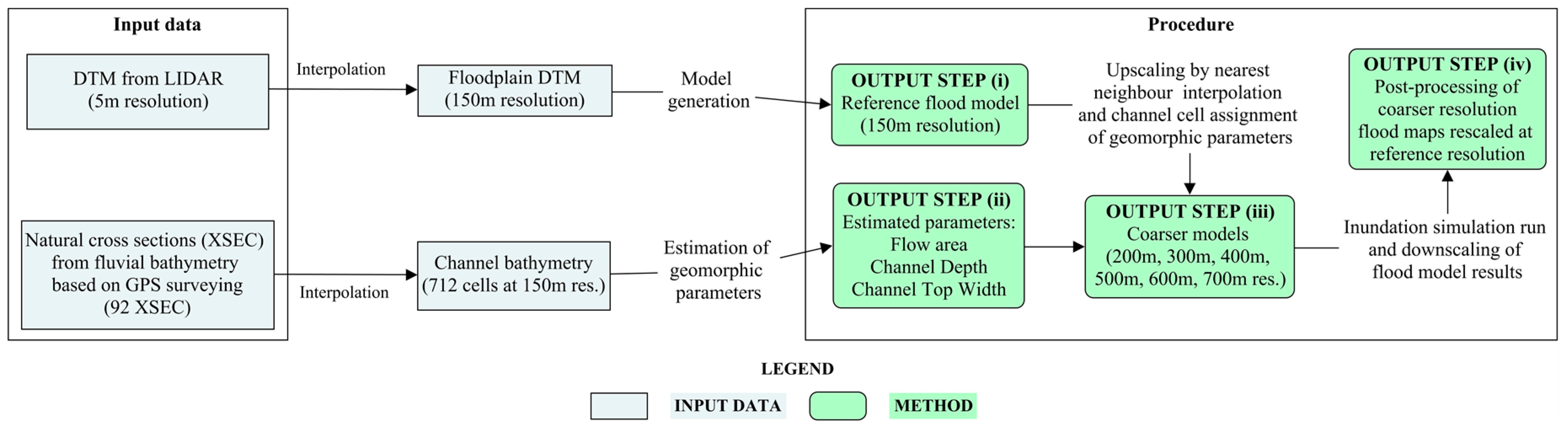
The implemented procedure was based on the following four steps:
(i) Building the 2D flood reference model at 150 m resolution
The high resolution 5 m DTM was interpolated at 150 m. The simulated inundation dynamics of the 150 m simulation were consistent to the original FLO-2D model gathered from the TRBM that was originally implemented at 50 m resolution. The 1D HEC-RAS model developed by the TRBA was used to gather the available 92 fluvial cross sections. The cross sections were imported into the FLO-2D model to assign a cross section to each of the 712 river channel grid cells. The FLO-2D channel geometry was created by linear interpolation of the original Hec-Ras cross sections. The 150 m flood model was evaluated to check that the floodplain DTM, channel cross section geometry and thalweg profile accurately match the original 50 m TRBM model.
(ii) Interpolation of natural cross sections to produce a synthetic rectangular channel bathymetric model
The 712 river channel grid cell elevations and associated cross sections were analyzed to estimate the channel cell-by-cell flow area, top width and channel maximum depth. The cross section depth characterizes the distance from top of the banks to minimum channel elevation defining the simulated thalweg profile of the fluvial channel. A rectangle was created to approximate each cross section. The channel bed elevation of the rectangle was estimated by subtracting the channel maximum depth from the DTM cell elevation to preserve the thalweg profile of the reference hydraulic model. The rectangle width was then varied to preserve the flow area estimated from the original cross section. Basically, the hypothesis was to define a rectangle that best approximates the surveyed cross section giving priority to the conservation of the channel slope (i.e., thalweg profile) and conveyance (i.e., flow area). The top width was used as calibration parameter in this channel bathymetry interpolation.
(iii) Upscaling flood model to coarser resolutions
The reference 150 m flood model DTM was upscaled to 200 m, 300 m, 400 m, 500, 600 m and 700 m resolution. The terrain analysis process generated coarser floodplain DTM resolutions based on the following steps: (1) Use high resolution 5 m DTM as input terrain model to interpolate the digital floodplain terrain for the flood model at the desired coarser resolution. (2) Identify the channel cells by proximity analysis of the 150 m reference channel model with the new coarser channel grid. (3) Associate to each channel cell the rectangle depth and height that preserve the average slope and flow area of the channel cells intersecting the coarser channel grid cell (as in Step (ii) above).
(iv) Inundation model runs and postprocessing of simulated water surface simulations
The coarse resolution model set up was used to perform the design event simulation representing the impact of the 200-year event on the fluvial domain. Flood modeling results were processed to depict the simulated water surface elevation, depth and velocities at the simulation resolution (200 m, 300 m, 400, 500 m, 600 m, and 700 m). The coarse resolution water surface elevation was interpolated at reference model resolution of 150 m. The simulated water surface was intersected with the high resolution DTM to produce the final inundation extent and flood depths. A postprocessing routine tool (freely available at https://github.com/antonioannis/FLO-2D-Processing-Tools) was used to interpolate and intersect the simulated coarse resolution water surface with the high resolution DTM. This analysis automatically downscaled the coarse resolution model inundating those floodplain cells that underlay the water surface elevation. Final results were plotted at 30 m resolution to allow better visualization of results. Figure 3 provides a schematic representation of the proposed procedure.
4. Results
The procedure is applied and results are presented in this section to depict the effect of the proposed floodplain terrain processing on flood modeling results with varying performances when upscaling the model from coarse to very coarse resolutions.
Figure 4 presents the results of Steps (i) and (ii) of the procedure by showing the cross section width, depth and flow area associated to interpolated synthetic rectangular cross sections at varying resolution with respect to surveyed cross sections of the reference model. It is shown how the channel bed elevation and flow area are preserved in all models for adjusted channel top width.
The simulated flood profile along the river channel is represented in Figure 5. The visual comparison shows that the six upscaled models have a consistent Water Surface Elevation (WSE) with discrepancies increasing with decreasing resolution. It is noted that the simulated surface seems always consistent even in some segments of the river reach where the spatial adjustment determines notable differences in the location of the bed profile. An underestimation of the water surface elevation is also noted when the channel slope is steep, while in the flat downstream valleys the differences decrease.
The simulated channel maximum discharge is reported in Figure 6. Here, the impact of the resolution on simulated floodplain flow dynamics is evident, considering that the expected impact of the different floodplain DTM realizations on the flood wave attenuation process. The use of synthetic cross section provides notable differences as well as the approximation of the channel bank elevation that plays here a major role, considering the importance of accurate river–floodplain exchange simulations. This result shows the significant impact of the resampling procedure on the simulation of flood wave propagation dynamics (i.e., discharge, velocities).
Results presented in Figure 5 and Figure 6 show that inundation simulations for the Tiber case study are not driven by peak discharge, but are mainly governed by flood volumes transiting along the valley. The maximum conveyance of the Tiber is not greater than 1000 m3/s, while the 200-year peak discharge is greater than 3000 m3/s for the entire domain. The consistency of flood profiles is motivated by the fact that, once the channel has reached its maximum conveyance capacity, the floodplain of the Tiber River acts as a large storage. The presented tests support the validity of consistent simulations of coarse to very coarse resolution models even in cases where the topography is represented using only 1–3 grid cells per floodplain cross sections. While it is expected that results of very coarse resolution will not match the accuracy of high resolution models for the reconstruction of flood wave dynamics, we posit that inundation extent and depths can be reasonably captured.
A significant advantage of the coarse resolution is the speed of the simulation and the computational efficiency. Table 1 shows the varying simulation computational performance with varying DTM resolutions. A summary of the main specifications of the different model set ups is provided with results also evaluating the total inundated area. The run time decreased from 37 min to 2.5 min using the same computer power (a regular workstation). Table 1 also includes the results of the measure-to-fit analysis with the F-index results.
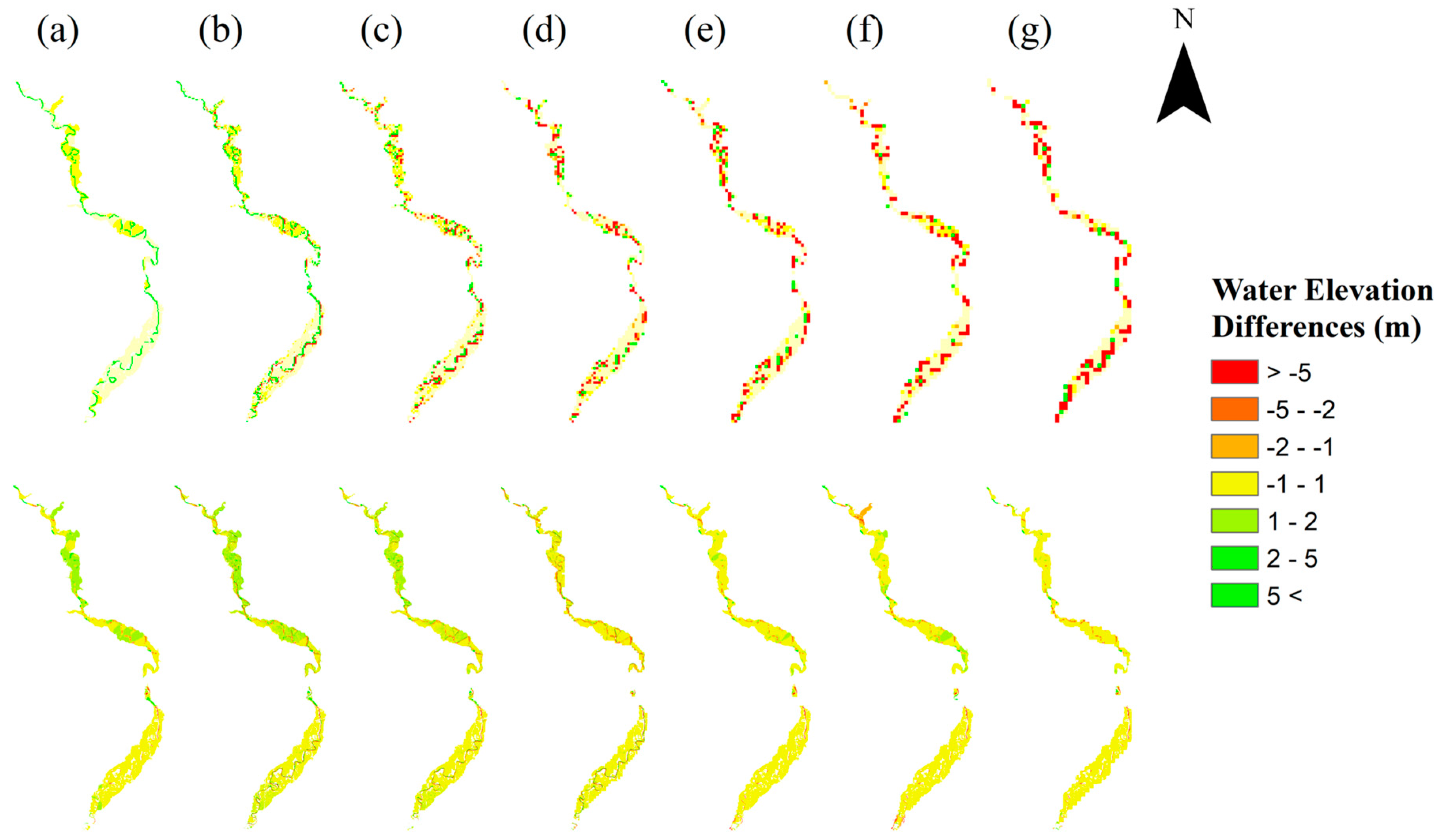
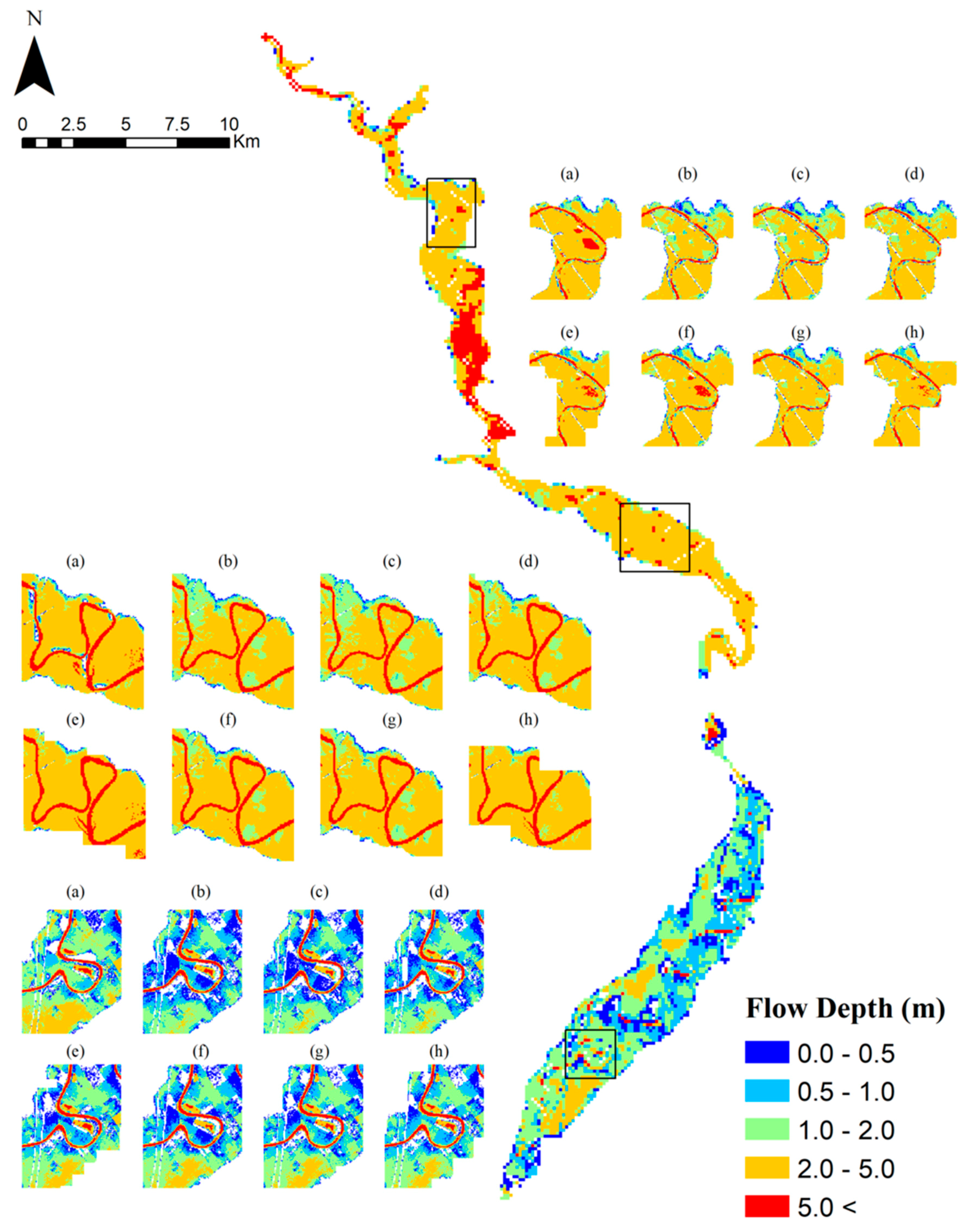
The visual comparison of simulated inundation depths is represented in Figure 7, Figure 8 and Figure 9. Figure 7 shows the differences between the simulated maximum floodplain flow depths at coarse (150 m) to very coarse (700 m) resolution compared to the reference model. The flood model resolution is maintained with no postprocessing here developed to show the visual effect of the varying resolutions. Figure 8 presents the spatial distribution of differences between floodplain maximum flow levels of the reference model compared to the upscaled flood simulation at different resolutions. Figure 9 shows the results of the simulated maximum flow depths from the reference 2D hydraulic model simulation for the entire study domain. Three insets are inserted into Figure 9 for zooming in on an upstream, central and downstream area of the model visualizing the comparison of simulated inundation depths for the different flood model resolutions. Note in Figure 8 and Figure 9 the use of the postprocessing tool of Step (iv) of the presented procedure for plotting high resolution simulated inundation maps.
5. Discussion
This research investigated the development of very coarse resolution 2D inundation numerical models supporting large scale flood mapping. A procedure for interpolating floodplain terrain and bathymetric data is proposed and tested with the goal of producing consistent inundation models using coarse resolution floodplain topography and synthetic representation of channel morphology. Results were evaluated compared to validated reference 2D flood models quantifying performance metrics of running time and distributed inundation extents and depths of coarse (150 m) to very coarse (700 m) hydraulic model simulations.
The proposed floodplain terrain analysis procedure for creating coarse resolution 2D inundation models, that are able to consistently simulate the inundation extent at large scale, may be beneficial for flood risk management in multiple ways. Fast and reasonably accurate 2D flood simulations, running in seconds or minutes at large scales, pave the way for the use of 2D models in early warning systems that commonly use 1D models. Coarse inundation models are also needed for implementing cross-disciplinary applications where hydrodynamic models are coupled with climatic (e.g., Global Circulation Models (GCM)), landscape evolution or ecologic models.
This research contributes to the development of alternative cost-effective parsimonious flood modeling approaches that can produce consistent results using largely available data, considering that floodplain morphology, and channel bathymetry specifically, is in constant change and measurements cannot be afforded periodically, becoming a challenge for both gauged and ungauged basins [43]. Results show that naturally surveyed cross sections can be replaced by synthetic geometry cross sections of rectangular shape maintaining a correct representation of channel slope (i.e., thalweg profile) and channel conveyance (i.e., channel flow area). This result links this research with large scale flood hazard modeling based on the use of geomorphic laws or literature values for providing valid estimation of morphologic parameters (river/floodplain width, depth and flow area) associated to varying climatic, geomorphic and hydrologic regimes [20,21,22].
This study also highlights the value of floodplain terrain analysis for processing high resolution DTMs to produce upscaled geometry for 2D inundation mapping. Flood model upscaling follows scaling principles that characterize inundation dynamics. The DTM scale (i.e., grid size resolution) shall be defined according to the scale of the simulated flood processes. A major river defining a large floodplain domain with flooding dynamics characterized by inundation widths and flow depths that are in the order of, respectively, kilometer (1–3 km) and meter (1–10 m) scale requires a proportional scale for the topographic and bathymetric representation. If this scaling principle is correctly applied, we argue that the loss of details in floodplain DTMs at coarser resolutions does not necessarily imply that simulated inundations will be affected by major errors. Fluvial bathymetry interpolation and floodplain terrain resampling, also using synthetic channel geometry, allow fast and accurate flood models (Figure 5 and Figure 6). Nevertheless, we cannot neglect that floodplain interpolation are difficult to be automated, but semi-automatic procedures are needed that require flood modeler interpretation, calibration and validation, especially when converting natural to rectangular shape cross sections.
The proposed procedure still requires, in fact, manual processing work by the flood analyst. Therefore, results can be sensitive to errors, time consuming activities and to subjectivity impacting the replicability and generalization of results. The full automatization of this procedure, integrating an objective analysis of the proper scale and resolution, for creating upscaled inundation models require further investigations using geomorphological laws for estimating rectangular cross sections. Moreover, the behavior of different numerical scheme of 2D flood modeling and the development of an extended set of case studies in other climatic and morphologic settings characterize future work needed for the generalization of the proposed procedure.
6. Conclusions
In this paper, a procedure of floodplain terrain analysis was introduced for supporting the development of coarse resolution inundation models. The procedure was tested for the 120 km domain of the Tiber River in central Italy to evaluate the consistency of simulated inundation extent and depth distributions, derived from 2D hydraulic models applying different floodplain DTM resolutions, as compared to a reference flood model that was validated in previous studies. The main conclusive remarks of this research are as follows:
- (1)
- The proposed floodplain terrain analysis procedure does not aim to replicate the performances of accurate high-resolution flood modeling that requires surveying of fluvial bathymetry and floodplain morphology. Flood hazard management for safe urban planning and risk mitigation requires detailed modeling of floodplain and urban features exposed to inundation risk. The aim of this research was to produce consistent coarse resolution flood models, running in seconds, for investigating applications where 2D inundation modeling is actually not used for its computational and data need burden. For example, this research may pave the way to the use of 2D inundation modeling in large scale real time emergency management operations or in the coupling of hydrodynamic models with climatic global circulation models, landscape evolution models or in continental ecologic modeling applications.
- (2)
- Results show the tests related to the substitution of surveyed natural fluvial cross sections with synthetic rectangular cross sections. The use of a synthetic channel geometry is a valid working hypothesis if the channel thalweg profile and flow area are preserved. The impact of channel geometry simplification on the inundation dynamics is evident, considering the importance of channel morphology on flood wave routing, with significant misinterpretation of simulated discharge and velocities. Nevertheless, simulated inundation extents and depths are modeled in the range of flood modeler expectations.
- (3)
- Visual representation of water depths and quantitative analyses, based on the use of a measure-to-fit F index, for evaluating the potential overestimation or underestimation of the flooding extent, show that the upscaling procedure produces consistent results of decreasing accuracy with increasing floodplain DTM grid size. Consistent inundation simulation results are obtained interpolating the floodplain DTM resolution from 150 m to 700 m. The running time of simulations is reduced by one order of magnitude from approximately 30 min to 3 min for the 700 m simulation.
- (4)
- The proposed procedure for flood model upscaling still requires expert knowledge and subjective manual processing of reference data for correctly interpolating DTM floodplain topographic and bathymetric data. Further research is needed for flood model calibration and validation towards the replicability and generality of the proposed procedure in other case studies.
Author Contributions
Francisco Peña (FP) and Fernando Nardi (FN) jointly conceptualized the research experiment, from the design of the procedure, to the presentation of results. FP gathered and processed the case study data, developed the floodplain terrain analysis and 2D flood modelling, wrote initial version of manuscript with tables and figures. FP and FN jointly produced the final version of the manuscript, figures and tables.
Funding
This work was funded by Regione Lazio Grant No. A11598 (Research grant “Media Valle del fiume Tevere”).
Acknowledgments
Reviewers and editors are acknowledged for their valuable comments that helped authors in significantly improving this manuscript. Antonio Annis is also acknowledged for providing technical assistance in the use of the FLO-2D postprocessing tool and for his support in the development of the Fit index analysis.
Conflicts of Interest
The authors declare no conflict of interest.
References
- Bates, P.D.; Horritt, M.S.; Aronica, G.; Beven, K. Bayesian updating of flood inundation likelihoods conditioned on flood extent data. Hydrol. Process. 2004, 18, 3347–3370. [Google Scholar] [CrossRef]
- Pappenberger, F.; Beven, K.; Horritt, M.; Blazkova, S. Uncertainty in the calibration of effective roughness parameters in HEC-RAS using inundation and downstream level observations. J. Hydrol. 2005, 302, 46–69. [Google Scholar] [CrossRef]
- Merwade, V.; Olivera, F.; Arabi, M.; Edleman, S. Uncertainty in flood inundation mapping: Current issues and future directions. J. Hydrol. Eng. 2008, 13, 608–620. [Google Scholar] [CrossRef]
- Di Baldassarre, G.; Schumann, G.; Bates, P.D.; Freer, J.E.; Beven, K.J. Flood-plain mapping: A critical discussion of deterministic and probabilistic approaches. Hydrol. Sci. J. 2010, 55, 364–376. [Google Scholar] [CrossRef]
- Domeneghetti, A.; Schumann, G.J.P.; Frasson, R.P.M.; Wei, R.; Pavelsky, T.M.; Castellarin, A.; Brath, A.; Durand, M.T. Characterizing water surface elevation under different flow conditions for the upcoming SWOT mission. J. Hydrol. 2018, 561, 848–861. [Google Scholar] [CrossRef]
- Ward, P.J.; Jongman, B.; Salamon, P.; Simpson, A.; Bates, P.; De Groeve, T.; Muis, S.; De Perez, E.C.; Rudari, R.; Trigg, M.A.; et al. Usefulness and limitations of global flood risk models. Nat. Clim. Chang. 2015, 5, 712–715. [Google Scholar] [CrossRef]
- Neal, J.; Dunne, T.; Sampson, C.; Smith, A.; Bates, P. Optimisation of the two-dimensional hydraulic model LISFOOD-FP for CPU architecture. Environ. Model. Soft. 2018, 107, 148–157. [Google Scholar] [CrossRef]
- Schumann, G.J.-P.; Bates, P.D.; Apel, H.; Aronica, G.T. Global Flood Hazard: Applications in Modeling, Mapping and Forecasting; American Geophysical Union and John Wiley & Sons: Hoboken, NJ, USA, 2018. [Google Scholar]
- Tauro, F.; Selker, J.; Van De Giesen, N.; Abrate, T.; Uijlenhoet, R.; Porfiri, M.; Manfreda, S.; Caylor, K.; Moramarco, T.; Benveniste, J.; et al. Measurements and observations in the XXI century (MOXXI): Innovation and multi-disciplinarity to sense the hydrological cycle. Hydrol. Sci. J. 2018, 63, 169–196. [Google Scholar] [CrossRef]
- Trigg, M.A.; Birch, C.E.; Neal, J.C.; Bates, P.D.; Smith, A.; Sampson, C.C.; Yamazaki, D.; Hirabayashi, Y.; Pappenberger, F.; Dutra, E.; et al. The credibility challenge for global fluvial flood risk analysis. Environ. Res. Lett. 2016, 11, 094014. [Google Scholar] [CrossRef] [Green Version]
- Jung, Y.; Merwade, V. Uncertainty quantification in flood inundation mapping using generalized likelihood uncertainty estimate and sensitivity analysis. J. Hydrol. Eng. 2012, 17, 507–520. [Google Scholar] [CrossRef]
- De Frasson, R.P.M.; Wei, R.; Durand, M.; Minear, J.T.; Domeneghetti, A.; Schumann, G.; Williams, B.A.; Rodriguez, E.; Picamilh, C.; Lion, C.; et al. Automated river reach definition strategies: Applications for the surface water and ocean topography mission. Water Resour. Res. 2017, 53, 8164–8186. [Google Scholar] [CrossRef]
- Vorogushyn, S.; Bates, P.D.; de Bruijn, K.; Castellarin, A.; Kreibich, H.; Priest, S.; Schröter, K.; Bagli, S.; Blöschl, G.; Domeneghetti, A.; et al. Evolutionary leap in large-scale flood risk assessment needed. WIREs Water 2017. [Google Scholar] [CrossRef]
- Price, R.K. An optimized routing model for flood forecasting. Water Resour. Res. 2009, 45, 1–15. [Google Scholar] [CrossRef]
- Gichamo, T.Z.; Popescu, I.; Jonoski, A.; Solomatine, D. River cross-section extraction from the ASTER global DEM for flood modeling. Environ. Model. Soft. 2012, 31, 37–46. [Google Scholar] [CrossRef]
- Bhuyian, M.N.M.; Kalyanapu, A.J.; Nardi, F. Approach to digital elevation model correction by improving channel conveyance. J. Hydrol. Eng. 2014, 20. [Google Scholar] [CrossRef]
- Leopold, L.; Maddock, T. The Hydraulic Geometry of Stream Channels and Some Physiographic Implications; Geological Survey Professional Paper; U.S. Department of the Interior: Washington, DC, USA, 1953.
- Lehner, B.; Verdin, K.; Jarvis, A. New global hydrography derived from spaceborne elevation data. Eos 2008, 89, 93–94. [Google Scholar] [CrossRef]
- Pappenberger, F.; Dutra, E.; Wetterhall, F.; Cloke, H.L. Deriving global flood hazard maps of fluvial floods through a physical model cascade. Hydrol. Earth Syst. Sci. 2012, 16, 4143–4156. [Google Scholar] [CrossRef] [Green Version]
- Andreadis, K.M.; Schumann, G.J.P.; Pavelsky, T. A simple global river bankfull width and depth database. Water Resour. Res. 2013, 49, 7164–7168. [Google Scholar] [CrossRef] [Green Version]
- Sampson, C.C.; Smith, A.M.; Bates, P.D.; Neal, J.C.; Alfieri, L.; Freer, J.E. A high-resolution global flood hazard model. Water Resour. Res. 2015, 51, 7358–7381. [Google Scholar] [CrossRef] [PubMed] [Green Version]
- Domeneghetti, A. On the use of SRTM and altimetry data for flood modeling in data-sparse regions. Water Resour. Res. 2016, 52, 2901–2918. [Google Scholar] [CrossRef]
- Tiber River Basin Authority. Piano Direttore dell’Autorità di Bacino del fiume Tevere (Flood Risk Management Plan); Autorità di Bacino del fiume Tevere: Rome, Italy, 2010. (In Italian) [Google Scholar]
- Spada, E.; Sinagra, M.; Tucciarelli, T.; Barbetta, S.; Moramarco, T.; Corato, G. Assessment of river flow with significant lateral inflow through reverse routing modeling. Hydrol. Process. 2017, 31, 1539–1557. [Google Scholar] [CrossRef]
- Manfreda, S.; Nardi, F.; Samela, C.; Grimaldi, S.; Taramasso, A.; Roth, G.; Sole, A. Investigation on the use of geomorphic approaches for the delineation of flood prone areas. J. Hydrol. 2014, 517, 863–876. [Google Scholar] [CrossRef] [Green Version]
- Tauro, F.; Olivieri, G.; Petroselli, A.; Porfiri, M.; Grimaldi, S. Flow monitoring with a camera: A case study on a flood event in the Tiber River. Environ. Monit. Assess. 2016, 188, 1–11. [Google Scholar] [CrossRef] [PubMed]
- O’Brien, J.S.; Julien, P.Y.; Fullerton, W.T. Two-dimensional water flood and mudflow simulation. J. Hydrol. Eng. 1993, 119, 244–261. [Google Scholar] [CrossRef]
- O’Brien, J.S. FLO-2D Users Manual; FLO-2D Software, Inc.: Nutrioso, AZ, USA, 2011. [Google Scholar]
- Sibson, R. A Brief Description of Natural Neighbor Interpolation; John Wiley & Sons: New York, NY, USA, 1981. [Google Scholar]
- ESRI. ArcGIS Desktop: Release 10; Environmental Systems Research Institute: Redlands, CA, USA, 2011. [Google Scholar]
- Grimaldi, S.; Teles, V.; Bras, R.L. Sensitivity of a physically based method for terrain interpolation to initial conditions and its conditioning on stream location. Earth Surf. Proc. Land. 2004, 29, 587–597. [Google Scholar] [CrossRef]
- Grimaldi, S.; Teles, V.; Bras, R.L. Preserving first and second moments of the slope area relationship during the interpolation of digital elevation models. Adv. Water Resour. 2005, 28, 583–588. [Google Scholar] [CrossRef]
- Merwade, V.; Cook, A.; Coonrod, J. GIS techniques for creating river terrain models for hydrodynamic modeling and flood inundation mapping. Environ. Model. Soft. 2008, 23, 1300–1311. [Google Scholar] [CrossRef]
- Brandt, S.A. Resolution issues of elevation data during inundation modeling of river floods. In Proceedings of the XXXI International Association of Hydraulic Engineering and Research Congress, Seoul, Korea, 11–16 September 2005. [Google Scholar]
- Da Paz, A.R.; Collischonn, W.; Tucci, C.E.M.; Padovani, C.R. Large-scale modelling of channel flow and floodplain inundation dynamics and its application to the Pantanal (Brazil). Hydrol. Process. 2011, 25, 1498–1516. [Google Scholar] [CrossRef]
- Jung, H.C.; Hamski, J.; Durand, M.; Alsdorf, D.; Hossain, F.; Lee, H.; Azad Hossain, A.K.M.; Hasan, K.; Khan, A.S.; Zeaul Hoque, A.K.M. Characterization of complex fluvial systems using remote sensing of spatial and temporal water level variations in the Amazon, Congo, and Brahmaputra rivers. Earth Surf. Proc. Land. 2010, 35, 294–304. [Google Scholar] [CrossRef]
- Biancamaria, S.; Bates, P.D.; Boone, A.; Mognard, N.M. Large-scale coupled hydrologic and hydraulic modelling of the Ob river in Siberia. J. Hydrol. 2009, 379, 136–150. [Google Scholar] [CrossRef] [Green Version]
- Merwade, V.; Saksena, S. Incorporating the effect of DEM resolution and accuracy for improved flood inundation mapping. J. Hydrol. 2015, 530, 180–194. [Google Scholar] [Green Version]
- Pappenberger, F.; Frodsham, K.; Beven, K.J.; Romanovicz, R.; Matgen, P. Fuzzy set approach to calibrating distributed flood inundation models using remote sensing observations. Hydrol. Earth Syst. Sci. 2007, 11, 739–752. [Google Scholar] [CrossRef] [Green Version]
- Nardi, F.; Morrison, R.R.; Annis, A.; Grantham, T.E. Hydrologic scaling for hydrogeomorphic floodplain mapping: Insights into human-induced floodplain disconnectivity. River Res. Appl. 2018. [Google Scholar] [CrossRef]
- Horritt, M.S.; Bates, P.D. Effects of spatial resolution on a raster based model of flood flow. J. Hydrol. 2001. [Google Scholar] [CrossRef]
- Aronica, G.; Bates, P.D.; Horritt, M.S. Assessing the uncertainty in distributed model predictions using observed binary pattern information within GLUE. Hydrol. Process. 2002, 16, 2001–2016. [Google Scholar] [CrossRef]
- Nardi, F.; Annis, A.; Biscarini, C. On the impact of urbanization on flood hydrology of small ungauged basins: The case study of the Tiber river tributary network within the city of Rome. J. Flood Risk Manag. 2018, 11, S594–S603. [Google Scholar] [CrossRef]
Figure 1.
Map of the study basin of the Tiber River in central Italy.

Figure 2.
The impact of varying resolution represented by floodplain topographic plan view and cross sections. The 5 m floodplain terrain model is compared to interpolated 150 m (left) and 400 m (right) resolution DTMs. The upper and bottom plots show, respectively, the horizontal and vertical displacement of the interpolated floodplain grid schematization and cross section as respect to the high resolution DTM.

Figure 3.
Flow chart describing the procedure implemented for interpolating the fluvial bathymetry and resampling floodplain terrain data to support coarse resolution flood modeling.
Figure 3.
Flow chart describing the procedure implemented for interpolating the fluvial bathymetry and resampling floodplain terrain data to support coarse resolution flood modeling.

Figure 4.
Plots of channel top width (a), depth (b) and flow area (c) using the different model set ups: from the 150 m reference model using the naturally surveyed cross sections to the seven realizations of the synthetic rectangular channel flood model for 150 m, 200, 300 m, 400 m, 500, 600 m and 700 m resolutions.


Figure 5.
River channel flow profile with simulated maximum water surface level at 150 m and coarser resolutions.
Figure 5.
River channel flow profile with simulated maximum water surface level at 150 m and coarser resolutions.

Figure 6.
River channel flow profile with simulated maximum peak discharge at 150 m and coarser resolutions.
Figure 6.
River channel flow profile with simulated maximum peak discharge at 150 m and coarser resolutions.

Figure 7.
Distribution of inundation flow depths for: (a) reference model at 150 m and natural cross sections; as compared to upscaled flood models synthetic rectangular cross section at resolution of: (b) 150 m; (c) 200 m; (d) 300 m; (e) 400 m, (f) 500 m; (g) 600 m; and (h) 700 m.
Figure 7.
Distribution of inundation flow depths for: (a) reference model at 150 m and natural cross sections; as compared to upscaled flood models synthetic rectangular cross section at resolution of: (b) 150 m; (c) 200 m; (d) 300 m; (e) 400 m, (f) 500 m; (g) 600 m; and (h) 700 m.

Figure 8.
Distribution of simulated surface water elevation differences for coarser resolution models against the reference model using the model resolution (top) and the postprocessed 30 m resolution (bottom) with: (a) 150 m; (b) 200 m; (c) 300 m; (d) 400 m, (e) 500 m; (f) 600 m; and (g) 700 m.
Figure 8.
Distribution of simulated surface water elevation differences for coarser resolution models against the reference model using the model resolution (top) and the postprocessed 30 m resolution (bottom) with: (a) 150 m; (b) 200 m; (c) 300 m; (d) 400 m, (e) 500 m; (f) 600 m; and (g) 700 m.

Figure 9.
Distribution of inundation flow depths of the reference model at 150 m resolution (full scale map) and three selected subdomains where inundation depths are depicted using the postprocessing geospatial algorithm for visualizing the different flood modelling scenario at 30 m model resolution comparing (a) reference model; (b) 150 m; (c) 200 m; (d) 300 m; (e) 400 m; (f) 500 m; (g) 600 m; and (h) 700 m.


Table 1.
Performance metrics of running time, maximum simulated inundated area and F-index comparing reference model with upscaled flood models at different DTM resolutions.
Table 1.
Performance metrics of running time, maximum simulated inundated area and F-index comparing reference model with upscaled flood models at different DTM resolutions.
| Grid Size (m) | Number of Cells | Running Time (min) | Inundated Area (m2) | F-Index (-) |
|---|---|---|---|---|
| REF | 11,191 | 36.97 | 125,370,000 | |
| 150 | 11,191 | 34.25 | 115,267,500 | 0.917 |
| 200 | 11,169 | 23.17 | 116,880,000 | 0.868 |
| 300 | 2838 | 6.53 | 122,400,000 | 0.825 |
| 400 | 1588 | 3.46 | 108,000,000 | 0.744 |
| 500 | 838 | 3.99 | 120,250,000 | 0.796 |
| 600 | 561 | 2.05 | 119,880,000 | 0.761 |
| 700 | 498 | 2.49 | 118,580,000 | 0.720 |
© 2018 by the authors. Licensee MDPI, Basel, Switzerland. This article is an open access article distributed under the terms and conditions of the Creative Commons Attribution (CC BY) license (http://creativecommons.org/licenses/by/4.0/).
Share and Cite
MDPI and ACS Style
Peña, F.; Nardi, F. Floodplain Terrain Analysis for Coarse Resolution 2D Flood Modeling. Hydrology 2018, 5, 52. https://doi.org/10.3390/hydrology5040052
AMA Style
Peña F, Nardi F. Floodplain Terrain Analysis for Coarse Resolution 2D Flood Modeling. Hydrology. 2018; 5(4):52. https://doi.org/10.3390/hydrology5040052
Chicago/Turabian StylePeña, Francisco, and Fernando Nardi. 2018. "Floodplain Terrain Analysis for Coarse Resolution 2D Flood Modeling" Hydrology 5, no. 4: 52. https://doi.org/10.3390/hydrology5040052
Note that from the first issue of 2016, this journal uses article numbers instead of page numbers. See further details here.