An Empirical Mode-Spatial Model for Environmental Data Imputation


1
Department of Civil and Environmental Engineering, Brigham Young University, Provo, UT 84602, USA
2
Department of Statistics, Brigham Young University, Provo, UT 84602, USA
*
Author to whom correspondence should be addressed.
Hydrology 2018, 5(4), 63; https://doi.org/10.3390/hydrology5040063
Submission received: 26 September 2018
/
Revised: 1 November 2018
/
Accepted: 13 November 2018
/
Published: 17 November 2018
(This article belongs to the Special Issue Water Quality Monitoring in Streams, Rivers, Lakes and Reservoirs: Novel Methods and Applications)
Abstract
:Complete and accurate data are necessary for analyzing and understanding trends in time-series datasets; however, many of the available time-series datasets have gaps that affect the analysis, especially in the earth sciences. As most available data have missing values, researchers use various interpolation methods or ad hoc approaches to data imputation. Since the analysis based on inaccurate data can lead to inaccurate conclusions, more accurate data imputation methods can provide accurate analysis. We present a spatial-temporal data imputation method using Empirical Mode Decomposition (EMD) based on spatial correlations. We call this method EMD-spatial data imputation or EMD-SDI. Though this method is applicable to other time-series data sets, here we demonstrate the method using temperature data. The EMD algorithm decomposes data into periodic components called intrinsic mode functions (IMF) and exactly reconstructs the original signal by summing these IMFs. EMD-SDI initially decomposes the data from the target station and other stations in the region into IMFs. EMD-SDI evaluates each IMF from the target station in turn and selects the IMF from other stations in the region with periodic behavior most correlated to target IMF. EMD-SDI then replaces a section of missing data in the target station IMF with the section from the most closely correlated IMF from the regional stations. We found that EMD-SDI selects the IMFs used for reconstruction from different stations throughout the region, not necessarily the station closest in the geographic sense. EMD-SDI accurately filled data gaps from 3 months to 5 years in length in our tests and favorably compares to a simple temporal method. EMD-SDI leverages regional correlation and the fact that different stations can be subject to different periodic behaviors. In addition to data imputation, the EMD-SDI method provides IMFs that can be used to better understand regional correlations and processes.
1. Introduction
1.1. Research Goals
This paper proposes an Empirical data imputation technique, called Empirical Model Decomposition, spatial data imputation (EMD-SDI) for time-series data based on an approach that decomposes signals into their component periodic parts, identifies correlated signals at other regional stations, extracts the missing part of the signal from these regional stations, and reconstructs the original signal from the component parts. Empirical Mode Decomposition (EMD) [1] is a signal deconvolution method that works with non-stationary, non-linear, quasi-periodic data; typical of environmental data series. Quasi-periodic data are data that exhibit cyclical changes without a precise period. EMD is data-driven and does not assume or require a stationary or linear signal. EMD decomposes a signal into a series of intrinsic mode functions (IMFs) each representing independent components of the signal and a residual representing the offset from zero and the overall trend in the dataset. Summing the IMFs and the residual exactly reproduces the original signal. EMD is sensitive to end effects. For this study, we did not select data gaps that were close to the end of the time series. The distance from the gap to the series end was at least the size of the gap. Methods to directly address this include either extending the data using the last value or mirroring the data. For earth sciences data, we contend that the best method would be to use data from the closest annual cycle to extend the data record.
We use EMD to decompose the signal from a target station into a finite number of IMFs, each an independent quasi-periodic signal [1,2]. Quasi-periodic data have a recurring cycle or oscillations that can occur at inter-annual, multi-annual, decadal, or longer times. We also decompose the signals from other stations in the geographic region (called source stations). As most environmental processes exhibit spatial correlation, we expect some of the IMFs from the source stations to have correlated quasi-periodic components [3]. After decomposing the data, we identify correlated IMFs from the target and source stations and use sections from the source IMFs most correlated with the target IMFs to reconstruct the missing section. We recreate the full signal at the target station using these reconstructed IMFs.
EMD-SDI data imputation can be used for any missing time-series data where regional datasets are expected to be spatially correlated or that exhibit correlated behaviors in time. Candidate data types that would appropriate for this technique include water quality, temperature, stream flow, precipitation, and other continuous processes of a periodic or quasi-periodic nature that exhibit spatial correlation [3]. Most earth observation data would be good candidates for this method. We demonstrate EMD-SDI on temperature data from the Utah Climate Data Center [4] with stations located throughout the state (Figure 1).
1.2. Background
Earth sciences, in disciplines such as hydrology or meteorology, use time series data to describe temporal processes such as water quality, streamflow, temperature, wind speed, solar radiation or similar processes. These data describe the environment and are analyzed to better understand, plan, manage, or control a wide variety of important hydrologic and environmental processes [5]. These data are generally semi-periodic and often non-linear and non-stationary (e.g., have a trend). While data are available from a number of sources that archive and provide environmental time-series data, nearly all these data sets have gaps or periods of missing data [6,7,8,9,10]. Studies have shown that missing data has adverse impacts to both modeling and analysis and that data estimation or imputation is required; see for example [6,9,11,12].
The literature reports a large number of data imputation methods. Much of the published work on environmental data imputation addresses methods for streamflow data, an area of research since the early 1960s [13]. While researchers have reported many advanced approaches in the literature, including combining EMD decomposition with Bayesian compressive sensing approaches [3]. Earth sciences often have data gaps and there are many different reported methods ranging from simple replacement [14,15], an offset method with only target site data which replaced a single missing value with averaged observed values before and after and for longer gaps used an average of the values from the previous and following year [16] (we used a simple version of this called the temporal method in this manuscript) to complex statistical models [17,18]; to spatial models [19,20]. Other methods include spatiotemporal models [21], pattern matching [10], and data modeling [22]. A large part of the published imputation work addresses streamflow or precipitation data and includes approaches such as spatial correlation with nearby sites [11,23,24,25,26,27], multivariate statistics [13,28,29]; Bayesian modeling [30], and models such as neural networks [5,31,32], chaos theory [33], and a Markov-chain Monte Carlo algorithm within a Bayesian modeling framework [20]. Our previous work used EMD decomposition as a preprocessing step, for a Bayesian compressive sensing approach to data imputation [3]. This method, while useful, is computationally intensive and difficult to implement. EMD-SDI, in contrast, is computationally fast and has a straightforward implementation. EMD and its extension, ensemble EMD (EEMD) have been in other earth sciences fields, such as runoff prediction [34,35,36,37].
Researchers have compared different methods [8,38,39,40] and reported that nearest neighbor methods were better than ARMA models for stream flow [41], that ANN approaches were better than ARMA models [42], and that ANNs performed better than linear regression [43] and nonlinear regression [44]. This is not a comprehensive literature survey as the field is large, but the references cited show the variety of work in this field and demonstrates that the “best” methods are dependent on the data.
Based on our personal experience and anecdotal discussions, most modeling studies use simple ad-hoc approaches such as using data from the closest station with simple offsets to fill data gaps—this approach seems to be especially true for temperature data, though we have no data or studies to support this statement.
We put forth EMD-SDI approach to address two issues: (1) advanced methods are difficult to implement and require parameters or information not readily available; and (2) often these methods do not provide estimates appreciably better than simple methods such as using data from the closest station to fill in gaps, thus earth science researchers continue to use ad hoc methods. Our approach is data-driven and only requires that a practitioner provide measurements from the region that have data over the same time period as the gap. Our work shows that this method generally out-performs methods such as using data from the closest station. In some respects, it is an automated version, where EMD-SDI defines the “closest” station as the one with the most correlated quasi-periodic processes rather than the one most geographically close.
1.3. Challenges
One significant challenge in data imputation is obtaining the data and information required. For example, in simple offset methods, you need to determine which station would be the best source for the data and determine the offset. The best choices are not always clear. In other methods, such as time-series modeling [16], model parameters have significant uncertainty and affect results. Even machine learning approaches and stochastic methods [31,33,43], model development is involved. Our approach, EMD-SDI, addresses this issue, as it is completely empirical. The user inputs available data for the target and source stations, the algorithm requires no additional parameters or tuning.
2. Data
2.1. Data Description
The Utah Climate Center at Utah State University archives data describing Utah climate. This archive contains daily environmental data collected at 815 locations throughout Utah for time periods ranging from December 1887 to the present. Each station records data with daily values of precipitation, minimum temperature, and maximum temperature. Some stations have additional data; however, nearly all these datasets are incomplete with gaps or missing data, the amount missing and the missing time periods depend on the station.
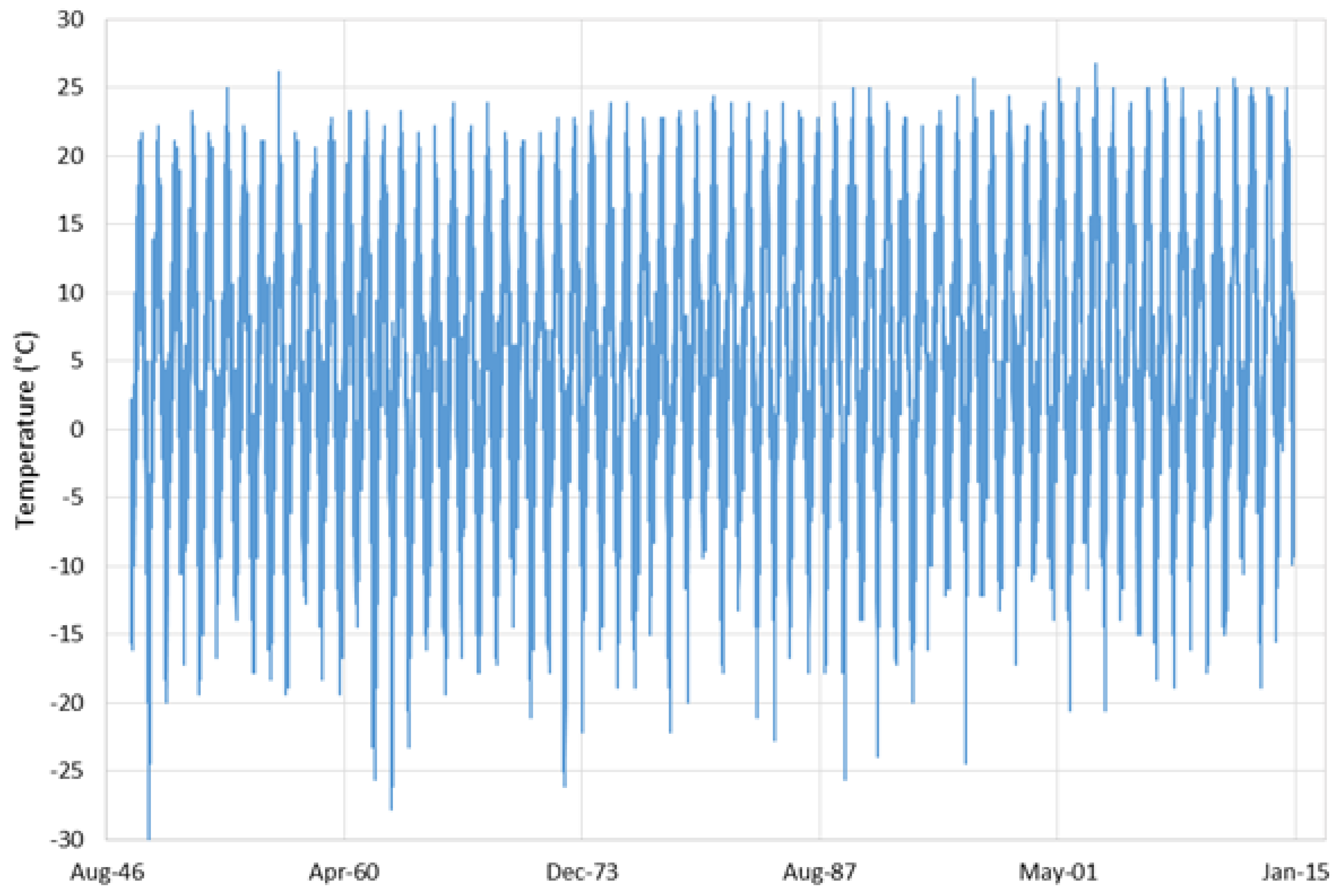
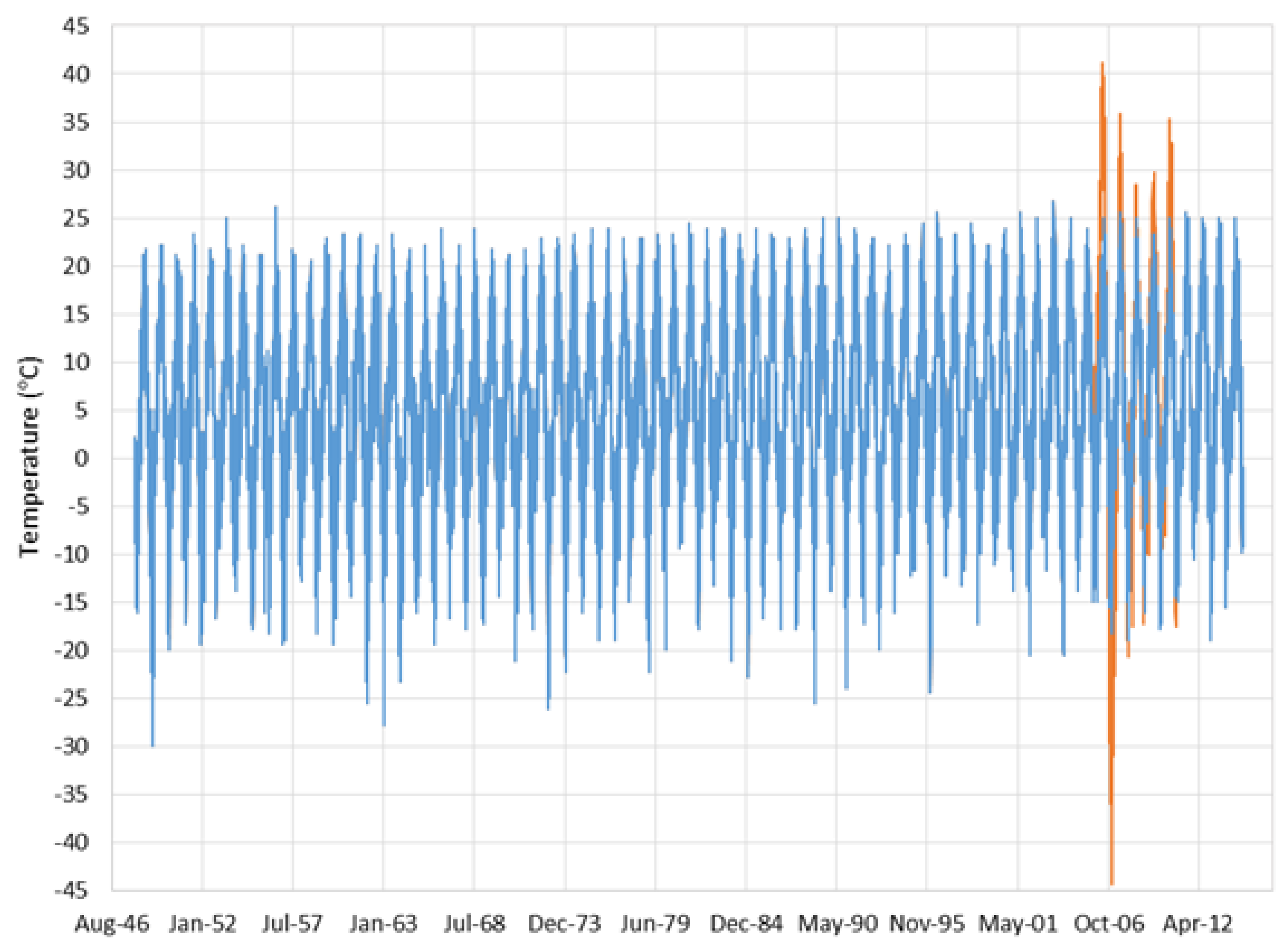
To test EMD-SDI, we used the daily minimum temperature set from Salt Lake International Airport (SLIA) station. We selected the SLIA station because it is the longest continuous dataset available, i.e., no missing data. This allowed us to remove data to generate gaps, and compare the imputed data with the original data to determine accuracy and performance. We used a variety of gap lengths and gap locations. Figure 2 shows the original SLIA data. Figure 2 shows that annual high temperatures are in a relatively narrow range, but annual low temperatures have more variance. We created gaps at random locations and different lengths, imputed data for those gaps, and compared the imputed data to the original, observed data. To impute the missing data, we allowed EMD-SDI to choose from either the daily maximum or the daily minimum temperatures from the regional stations as potential sources.
2.2. Data Parsing and Cleaning
The amount of data and dataset lengths available at the other 814 stations varies. Many stations contain only precipitation data or only contain a few days of temperature data. We performed some initial data processing to select reasonable stations for this study and to prepare the data for processing.
Data parsing and cleaning consisted of two activities; the first was selecting which sites to include in the study. We evaluated the 814 stations and selected about 450 stations to include in this study based on if they had sufficient data. We set the minimum data length to 1 year. We also removed stations if they did not contain the temperature information (i.e., maximum and minimum values). After site selection, we processed the data by removing clearly inaccurate data. These inaccuracies likely came about due to poor management or recording of the data. The first stage of preprocessing involved removing data points indicating a daily high temperature greater than 50 °C (Utah record high is 47 °C), or a daily low temperature lower than −60 °C (Utah record low is −56 °C). Afterwards, we removed data points if the daily high value was lower than the daily low value. This removed most of the extreme values but did not address errors such as seasonal temperatures that were clearly inaccurate, for example, a 30 °C day in the middle of winter. To solve this problem we computed temperature distributions for each day of the year for each station. We then used the interquartile range (IQR) and the 1st and 3rd quartiles to identify outliers on any given day. Since we did not want to remove all outliers, only those that were clearly inaccurate, we determined an offset, o, and multiplier, m, for the IQR and excluded values outside that range as erroneous outliers. Based on a visual analysis, we determined that a reasonable value for the multiplier, m, and offset, o, were 1.75 and 8 respectively, so for our data we considered anything greater or less than 14 times the yearly-day average as an outlier and it was removed. The resulting data sets all had data gaps, both from the original record and from data removed during pre-processing. After the station selection and data cleaning, 408 temperature stations were available and used in this study. Each station had maximum and minimum temperature time-series records and all had varying numbers of gaps with varying lengths.
We used MATLAB to import and analyze the data, select the stations to use, parse the data, perform preprocessing procedures, and format the structure for further analysis. We created a MATLAB data structure to store the data sets, which included both the temperature time-series data and various meta-data necessary for processing. We extended each data set to be the same length so that each data set started and ended on the same day. To accomplish this we extended each time series and created a Boolean mask to identify these locations as missing data values so they would not be included in the processing or considered by the EMD-SDI algorithm.
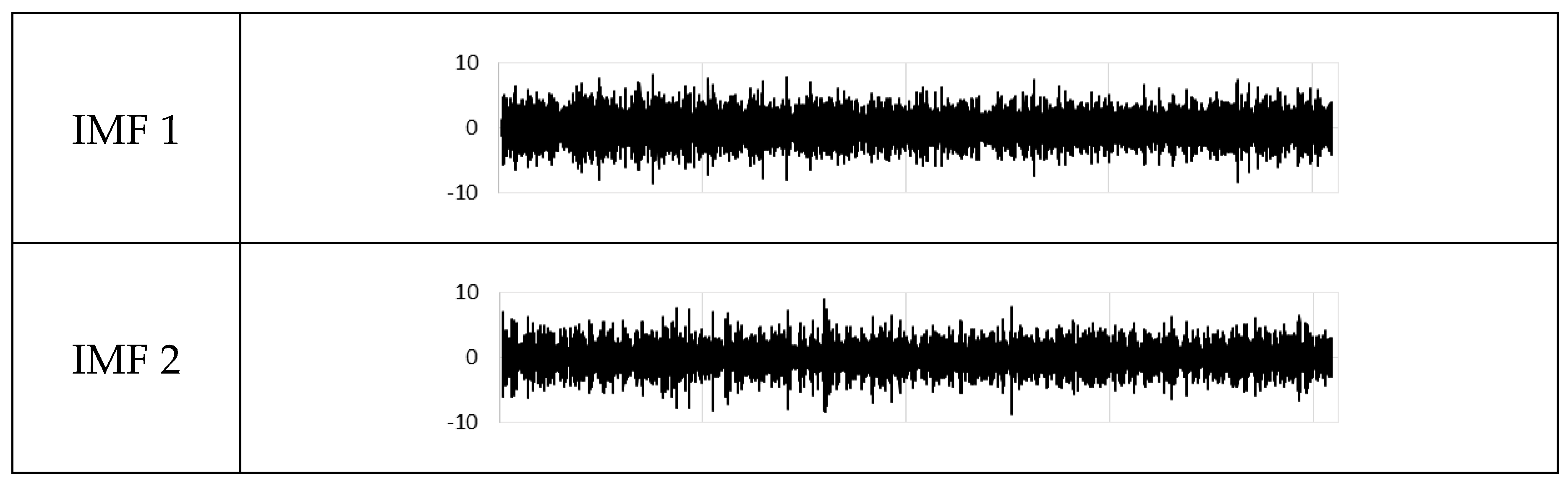
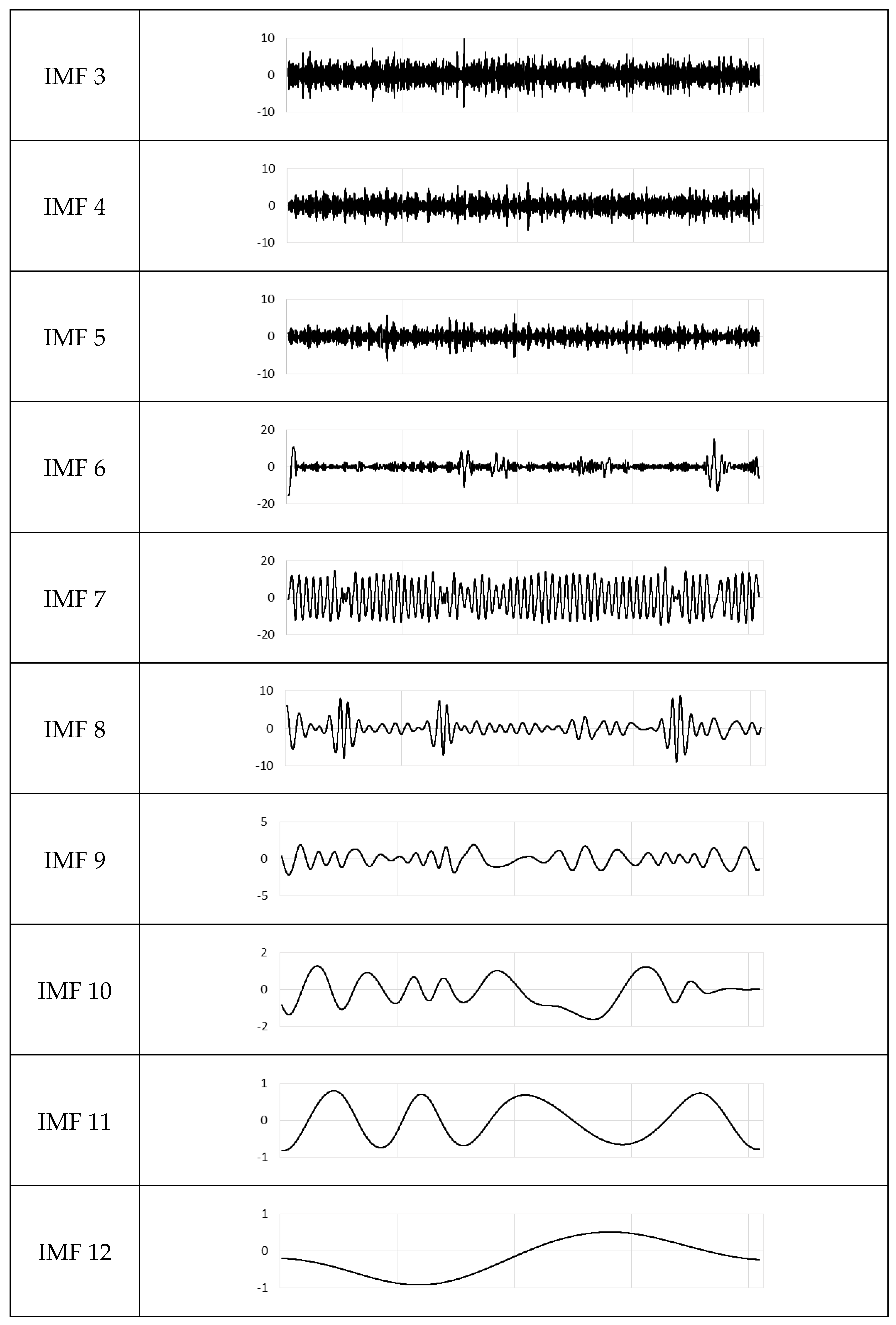
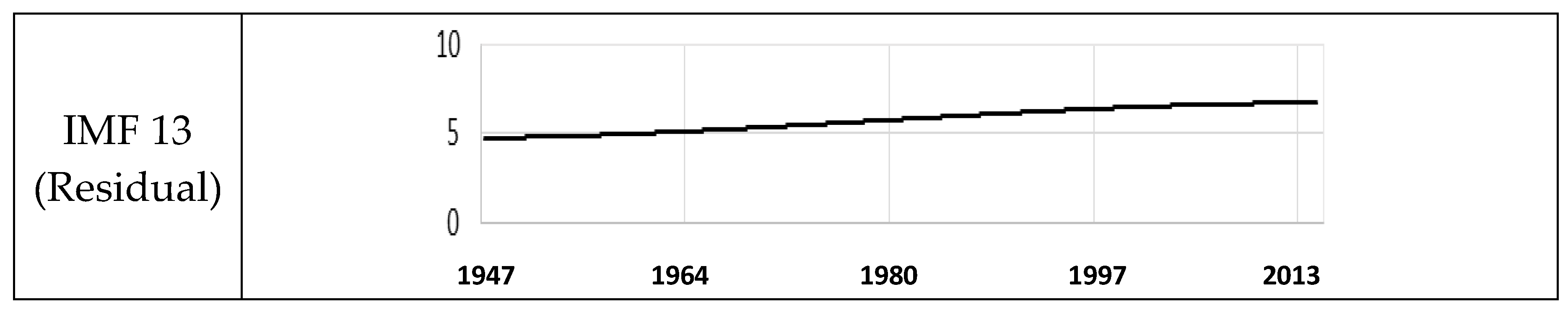
Figure 3 shows a set of example IMFs from the SLIA station data. The first five IMFs range from about −5 to 5 and seem to present noise in the data—though this assertion is only based on a visual examination. The next three IMFs (IMF 6–8) range from about −15 to 15 and have about a 1-year or annual period. IMFs 9 could be from the El Nino patterns, while IMFs 10–12 represent longer periods and may or may not represent actual physical processes. The final IMFs, IMF 13 is called the residual. The residual represents the long-term trend for the data. This example shows a small increase over the data set.
3. Methods
3.1. Description
EMD is a novel data analysis technique first published in 1998 [1]. The EMD algorithm decomposes nonstationary and nonlinear signals. Common decomposition techniques such as Fourier decomposition or wavelet analysis cannot be applied to nonstationary and nonlinear processes; nonstationary and nonlinear data are common in environmental data sets. The EMD approach, in contrast, assumes that data are composed of independent signals with simple intrinsic modes of oscillation. The EMD algorithm is adaptive and defines the basis functions used for decomposition on an a posteriori rather than an a priori basis, both Fourier transforms or wavelet analysis use a priori basis functions [1]. EMD decomposes a signal into basis functions called IMFs. An important trait of EMD, as with any signal decomposition approach, is that the summation of individual components recreates or approximates the original time-series dataset. Unlike Fourier transforms, recreating a signal by summing the resulting IMFs results in the exact original data—not an approximation. We used existing EMD code [45] that implemented cubic spline interpolation for the splining procedure and default stopping criteria. We modified the code to use a pchip interpolation function to eliminate over- and under-shot in the interpolation.
EMD identifies independent quasi-periodic phenomena using an empirical approach based on the data, rather than a pre-selected form such as a wavelet function. The resulting components or IMFs, in many cases, have been shown to represent naturally occurring processes such as the El Nino/La Nina cycle or sunspot influences [46]. Our experience has shown that while some of the IMFs are consistent with natural quasi-periodic processes, others seem to represent more random, but time correlated processes. While the resulting IMFs may not be related to any natural processes—we assume that these components will appear in other regional stations and be time-correlated with each other, whether they represent natural processes that influence the system—such as the El Nino/La Nina cycle—or other random processes. We assume that the temperature data are spatially correlated and that similar processes, represented by the IMFs, will appear in data from other regional stations.
EMD-SDI decomposes the target signal and potential source signals into IMFs, then using periods before or after the data gap finds the best match (e.g., highest correlation) to the individual target IMFs in the source IMFs. We use the selected source IMFs to fill the data gap. Other EMD-based imputation methods have attempted to model the complicated behavior that takes place within a natural process which is more complex and difficult to implement [47]. We assume that the data in the source stations are correlated with the target station because the earth sciences processes we are interested in, e.g., temperature, water quality, stream flow, etc. are spatially correlated.
In our example, we evaluate all the IMFs from the candidate stations (the 408 stations with sufficient data to include in the study) to find the IMF most similar to the IMF in the subject station (SLIA). We repeat this process for each IMF from the decomposed SLIA station signal. We assume that if these IMFs represent natural processes, then other stations should also exhibit the same behavior and have a matching IMF. For IMFs that represent random time-correlated processes, we assume that other stations, subject to a similar environment, may also exhibit a similar random signal. Since temperatures in similar geographic regions follow similar trends over time, we should be able to fill gaps by identifying stations that have an IMF with a similar natural frequency as the station in question for the time period for which data are missing. This approach is similar to a commonly used method in hydrology where a station close to the station with missing data is identified (candidate station), the data offset between the two stations is determined, and gaps are replaced by data from the candidate station plus or minus the offset. The difference, in this case, is that we may use several stations to reconstruct the missing data and reconstruct each IMF separately. One benefit from using the EMD processing is that that the residual trend, which represents the offset from zero in the data, is the final step in recreating the signal and is a smooth function. All the IMFs are centered on zero, which allows for matching quasi-periodic signatures without matching magnitudes or offsets. It also means that, for example, a close station may be at a significantly different elevation and have very different actual temperatures than the target station; however, since both stations may be subjected to similar microclimates such as lake effects, they may have similar quasi-periodic processes imbedded in the temperature signal that can be leveraged by EMD-SDI.
3.2. Imputation Process
3.2.1. Process Overview
For discussion, we will call the signal to be filled, the SLIA station, the target station. We will designate the other stations as candidate stations. For an actual application, you would begin by identifying gaps in the target station. For our example, we created data gaps in the SLIA data to evaluate how well the algorithm worked. This approach allows us to use the removed data as truth in evaluating the imputed data.
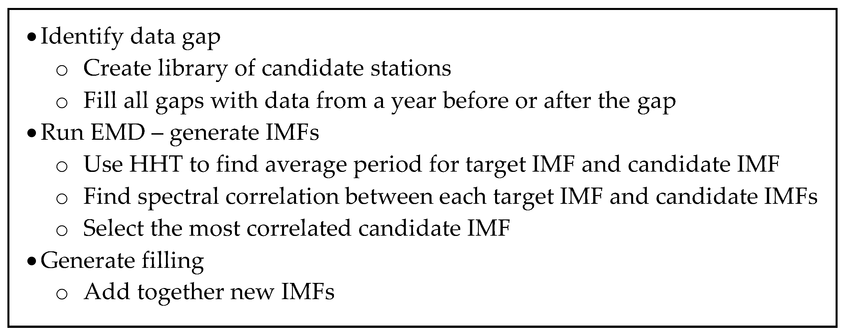
The EMD-SDI algorithm decomposes both the target and candidate stations into IMFs, finds the best match to the target IMFs within the full candidate IMF library, replaces the missing data in the target IMF with the selected candidate IMF, then reconstructs the original signal using these “filled” IMFs. This process is outlined in Figure 4.
3.2.2. Preliminary Gap Filling—Temporal Data Imputation
EMD works best with continuous data, so prior to running the EMD algorithm; we filled any gaps with temporary data. While the EMD algorithm can run on data with gaps, temporarily filling the gaps makes the algorithm more efficient and reduces the possibilities of over- and under-shooting, as EMD is sensitive to abrupt discontinuities. For these temporary data, we used data from the same time periods in the years before and after the gap to fill the initial gaps. This simple data imputation method is often used with earth science data [16] and later in the paper, we will compare the EMD-SDI results to using this temporal method to fill the gaps in the SLIA data set.
3.2.3. EMD Application
We first applied the EMD algorithm to both the target and candidate stations to provide a set of target IMFs and a library of candidate IMFs for matching and data imputation. After we decomposed the signals into IMFS and generated the candidate stations IMF signal library, we examined each IMF from the target station using the Hilbert Huang Transform (HHT) [1]. The HHT computes the instantaneous frequency of the IMF. This is similar to determining the frequency of each component in a Fast Fourier transform (FFT) decomposition. However, the frequency of an IMF can change with time unless the process is strictly periodic. The HHT estimates the frequency of the IMF at each point in time and as a practical note, the HHT results exhibit significant noise. Using the HHT data, we computed the average instantaneous frequency and instantaneous period for each IMF; similarly, we determined the average instantaneous period for each library signal. We then compared the statistics for the target IMF with the IMFs in the library. If the difference in the average instantaneous frequency or period of a candidate IMF was smaller than two times the instantaneous period of the target signal, we retained that IMF for further analysis. We performed this step to reduce the number of candidate IMFs evaluated.
3.2.4. Matching Signals
From this resulting set of candidate IMF signals, we determined the one most correlated with the target IMF. To determine the most correlated IMF, we used various goodness of fit metrics to evaluate the fit between the target IMF and the candidate IMFs. There are many different ways of measuring the match or correlation between quasi-periodic signals. We evaluated several methods including Normal Euclidean Distance (NED), Spectral Angle Coefficient (SA), Spectral Correlation Coefficient (SC), and Spectral Gradient Angle (SGA). We define these methods in the following equations where:
x = target IMF
y = candidate IMF
The Normal Euclidean Distance (NED) is defined as:
For NED = 0 indicated perfect correlation [48].
The Spectral Angle (SA) is defined as [48]:
where represents the dot product of the two vectors.
We modified the SA equation so that the best match was the largest rather than the smallest number, the modified equation is:
The Spectral Correlation (SC) coefficient is defined as [48]:
Values of the SA, SGA and SC have a range of (−1, 1), with 1 representing perfect correlation, and −1 representing data exactly out of phase.
We evaluated these error metrics to determine which was most sensitive to the features of interest, which was the shape of the IMF. We found the SA was consistently the best for quantifying the fit in amplitude and frequency between the two IMFs. While the SA does not encompass all the important aspects of a signal, it seems to identify the correct candidate IMFs for this task.
We used the SA error metric to determine the most correlated IMF from the candidate IMFs. In practice, the SA value for the highest correlated IMF had a large range, from relatively low values (i.e., 0.2–0.3) to high values that indicated very good matches (i.e., greater than 0.9). We found that it was difficult to match the trend (the final or residual IMF), as the SA indicates a good match even if the data are shifted in magnitude.
3.2.5. Reconstruction
After we have identified the best match for each target IMF using the Spectral Angle metric, we used the portion of the candidate IMFs associated with the gap to impute the missing portion of the target IMF. We continued this process for each target IMF and then reconstructed the target signal by summing these constructed IMFs.
4. Data Imputation Example
4.1. Case Study Description
We tested our method on the data from the SLIA station by generating a number of synthetic gaps of varying lengths at different times in the record. This allowed us to compare our imputed data to the observed record. We used 6 different gap lengths: 30 days (1 month), 180 days (6 months), 365 days (1 year), 730 days (2 years), 1095 days (3 years), and 1825 days (5 years). While it is unlikely that we could accurately impute data over a 5-year gap, it is helpful for demonstration.
We generated 10 realizations for each gap length, randomly selecting the location of the missing data. For the longer time periods, not all the random realizations were successful as the location of the data gaps did not allow our algorithm to perform the initial data filling because the gaps were too near the beginning of the data set. For gaps longer than one year, we used data from several previous years. If the data period before the gap was shorter than the gap, we generated another realization. We could have used data from subsequent years, but we did not implement this option, as it was more efficient to generate another realization.
The algorithm selected IMFs for imputation from across Utah. SLIA has an elevation of about 4200 feet above sea level. Stations used for imputation included data from stations at Hill Air Force Base (about 30 miles north of SLIA and in a similar setting), Dugway Proving Grounds (about 100 miles west of SLIA in a flat desert setting with a similar elevation), Flaming Gorge Reservoir (about 200 miles east of SLIA in very mountainous terrain at about 6000 feet), Heber (about 50 miles southeast of SLIA in a mountain valley at about 5600 feet), Garrision (over 200 miles south-west of SLIA at an elevation of about 5300 feet), Parowan (about 230 miles south of SLIA at an elevation of about 6000 feet), Kanab (about 300 miles south of SLIA at an elevation of about 5000 feet in red-rock canyon settings), and Myton (about 150 miles west of SLIA across the Wasatch range in a valley of the Uintah range at about 5000 feet elevation). Different runs selected data from different stations, but these stations were often located at large distances in environments very different from SLIA.
4.2. Case Study Results
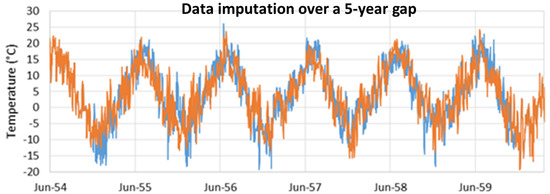
Figure 5, Figure 6, Figure 7, Figure 8, Figure 9 and Figure 10 show the results from the first realization for each gap length. We randomly selected the gap locations as can be seen by the dates on the x-axis. In each figure, we selected the x-axis range to match the data gap size to better show details. The blue line represents the original data and the orange line is the data generated by the EMD imputation method.
While there is a varying degree to which the generated signal represents the original signal, we observed that for the most part the algorithm is doing what is expected. All the generated signals approximately match the time location of relative minima and maxima across the signal. This is especially true for the signals in Figure 5, Figure 6 and Figure 7 that show more detail. While there are locations where the generated data may shoot above or below the actual data, with no a priori knowledge and using only visual inspection, we find that the generated signal closely models the original data.
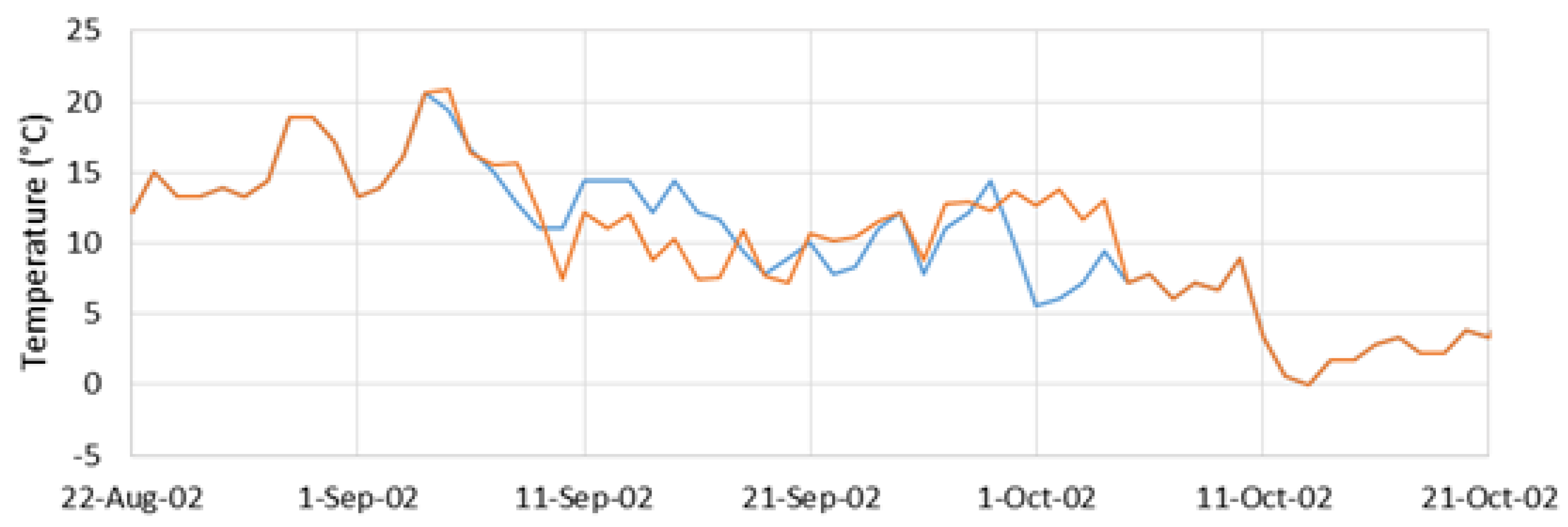
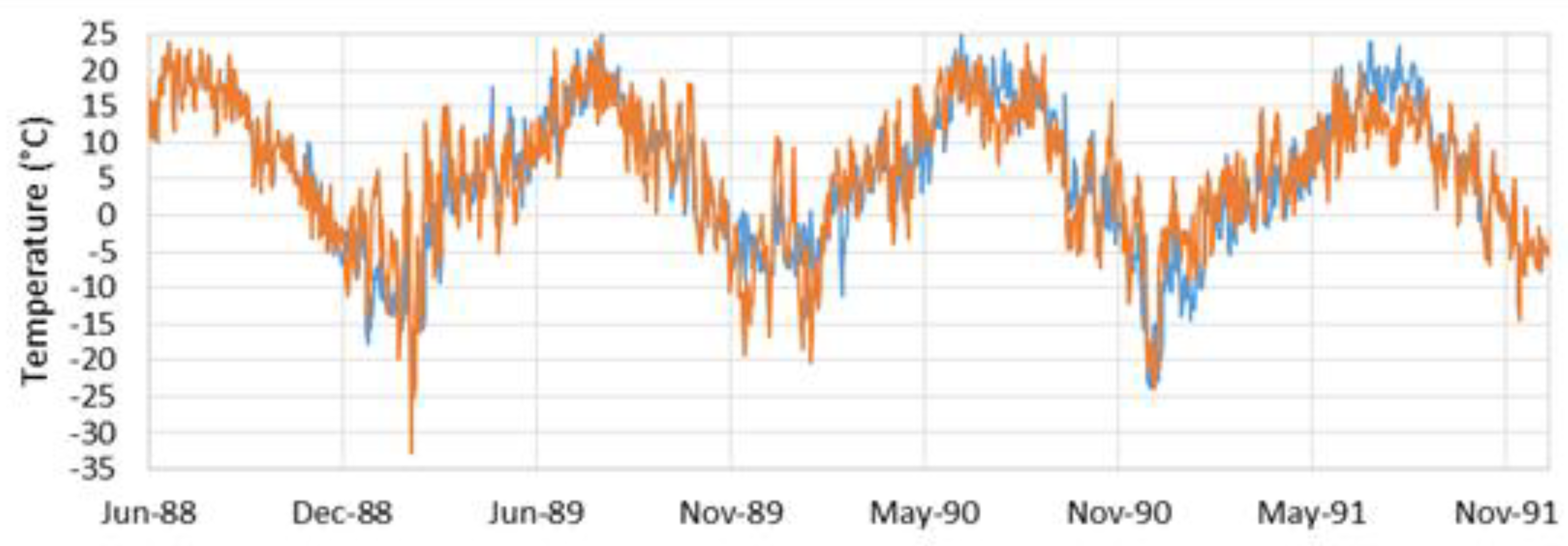
Figure 5, Figure 6, Figure 7, Figure 8, Figure 9 and Figure 10 visually show that the imputed data match the general trends and values of the observed data. In the longer gaps, Figure 5, Figure 6, Figure 7, Figure 8 and Figure 9 the imputed data recreating the annual cycle and also do a good job of matching short-term fluctuations, on the order of a few days. In Figure 7, with a 365-day (1-year) gap, there is are two periods, one in May and one in June, where the imputed data over-predict the temperatrues, but overall the fit is remarkably good. Figure 8 shows that over the 1095-day (3-year) gap, the imputed data match the seasonal variations and does a good job on the shorter fluctuations. But it does not accurately match the extreme low temperature in the winter of 1988, while it does a good job on the other years. Figure 10 shows results from the first realization of data imputation over a 1825-day (5-year) gap. Again, the seasonal variations are recreated well, however the imputed data are significantly colder in the winter of 1955, with a few outlier cold days in the winter of 1957. The general fit is remarkable for such a long gap.
4.3. Data Imputation Comparison
In this section, we present quantitative fit metrics for all 10 of the realizations for each gap length. We used Root Mean Squared Error (RMSE) and SA as the error metrics to determine the goodness of fit between the imputed and observed data. As the results were comparable, we only present the RMSE values in the following tables.
We also compared our method, EMD-SDI, with the simple imputation method used for the initial gap filling prior to running the EMD algorithm; we call this method the “temporal” method. The temporal method imputes missing data using data from the same station but from the previous annual period [16].
RMSE is defined as:
where is the data value from the original signal and y is the data from the generated signal. We computed the RSME and Spectral Angle metrics for each of the two different methods for all the completed realizations. The Spectral Angle metric and RMSE metric, while generating different values, created the same results. That is, if the RMSE indicated one method was best, the Spectral Angle metric indicated the same. In Table 1, we only present the RMSE values. Table 1 summarizes the different realizations for each gap length. Table 1 includes the median, maximum, and minimum RMSE values for each ensemble of realizations along with the number of successful trials. A trial was successful if the EMD-SDI method resulted in a better RMSE value than the temporal method.
In these tables, we report the median value rather than the mean, because large outliers significantly influence the mean value and we felt that the median better reflected the performance of the imputation methods [49].
The shortest gap, 3-months, had 10 out of 10 successful realizations, with the 3-year gap only having four successful realizations out of 10. The 6-month gap had 5 out of 5 successful realizations, all the other gap-lengths had more successful than unsuccessful realizations.
The EMD-SDI method has a lower median RMSE value for all gap lengths, except for the 3-year gap. However, even though this indicates that the EMD-SDI method out-performs the temporal method, in every case but the shortest gap, the maximum RMSE value is higher for the EMD-SDI method than for the temporal method. Therefore, while on average, the EMD-SDI method out-performs the temporal method, there is a larger variation in the results. This is because in some realizations, while the individual candidate IMFs correlate well with the target IMFs, they can “constructively” interfere, resulting in either very low or high values, often exceeding the data limits of the target station. There may be methods to address this issue. One potential solution would be to use determine the distribution of flows on each day, if the imputed data exceeded some level, for example, three standard deviations, the imputed value could be scaled back toward the mean by some multiplier. We did not attempt to implement such an algorithm. In some cases, larger variations in the imputed results may be beneficial as these realizations are generally conservative, resulting in more extreme values.
Figure 11 shows the 3-year gap realization with the largest large RMSE value, 8.64. The plot clearly shows the imputed data exceeding the data envelop of the target station, though the shape and general visual fit of the imputed data are good. On approach to address this issue would be to clip or restrict the imputed data to the existing data envelope to eliminate the unrealistic values. However, this would change the shape of the annual cycle. More sophisticated could be developed that scaled the data based on how far out of envelope the values were. This would retain more variability in the imputed data without significantly exceeding observed limits.
This issue of over- or under-shoot is not present in the temporal method, as the temporal method only uses existing data from the data record. While overall, EMD-SDI results were acceptable, as indicated in Figure 5, Figure 6, Figure 7, Figure 8, Figure 9 and Figure 10, and had lower median RMSE values, for some of the realizations the imputed data had significant over- or under-shoots, as indicated by the maximum RMSE values that exceed those of the temporal method. More importantly, these realizations often produced unusable data that is the imputed data are outside the observed range often resulting in physically improbable temperatures.
While the shortcomings of the EMD-SDI method could be addressed to eliminate these issues, the generally good performance of the temporal method raises the question of whether complex data imputation methods, such as EMD-SDI, are necessary even though EMD-SDI only requires regional data sets.
As noted in the introduction of this paper, there is a significant amount of published literature on advanced data imputation methods for the earth sciences and, as noted, these methods are not commonly used by most practitioners. We argue that advance data imputation methods have a place and that research should continue into this area. As demonstrated, EMD-SDI on average performs significantly better than the temporal method, if the algorithm is adjusted to address out-of-envelop imputed data, then EMD-SDI provides several benefits, it is easily implemented, only requires data from surrounding stations, and could provide researchers and practitioners with a more accurate imputation method.
5. Conclusions
In many regions, there are large amounts of earth observation data. However, data at any given site are often incomplete, with gaps and missing data. Earth processes are usually spatially correlated, however, the station closest in distance, may not be the station most correlated with the target station. The EMD-SDI method decomposes earth observation time series data into a set of independent quasi-periodic signals; then searches the entire set of signals for those that are most correlated to the target station to impute the missing data. This leverages spatial correlation in quasi-periodic processes that might not be obvious using other techniques.
The EMD-SDI technique for data imputation performed very well, credibly imputing data across gaps as long as 5-years. On average it out-performs the temporal method, though in some cases the imputed data exceed the observed data envelop and the temporal method performs better. Even in these cases, visual examination shows that the imputed data closely follows the temporal patterns. We believe the further research could address these shortcomings.
EMD-SDI shows promise and on average out-performed the temporal method. However, it is questionable if the additional complexity of EMD-SDI provides enough benefit for practitioners to use this method. While we would like to answer in the affirmative, in reality at this point the algorithm will not likely be chosen in practice.
It is important to present this work, even if EMD-SDI might not be a clear alternative, for two reasons, EMD methods highlight different aspects of the data. We showed that the algorithm selected source stations geographically distant from target stations. This highlights underlying processes in a region. Knowing these exist, additional insights might result. Below we suggest potential improvements to the EMD-SDI algorithm. It is likely that these improvements will increase the accuracy of the method and provide justifications for its use.
Future Work
We have several approaches we would like to explore to address the issue of over- and under-shoot in the imputed data. The simplest would be to simply scale any imputed data that exceeded the bounds of the target station as discussed above. Another potential method is to iterate the imputation procedure; we think that this process would converge on a more accurate signal. There are other potential solutions, but we believe this has the greatest potential.
While there are a significant number of data imputation methods for earth observation data, they are not widely used. We believe one of the hurdles to wider use, is the issue of parameterization, often requiring assumptions or data not readily available. EMD-SDI does not require the user to make any assumptions, the process is data-driven. Another obstacle to wider adoption of data imputation methods is implementation. For example, the EMD-SDI method, while relatively simple in principle, requires a significant amount of code to perform the data manipulation and search functions. Many practitioners and researchers do not have the resources to re-implement these algorithms. We feel that data imputation researchers, once they have developed an algorithm that performs better than simple methods, should provide example implementations and make them available to the community. For us, this is an area of future work.
Author Contributions
G.P.W. and C.B. conceived the EMD-SDI algorithm and evaluations; B.N. implemented the algorithms and performed the analysis, D.A.W performed the initial data collection and processing and assisted in the algorithm evaluation process. G.P.W. and B.N. were the primary authors of the manuscript with significant input from D.A.W. and C.B.
Funding
This work was supported by the National Nuclear Security Administration Department of Nuclear Nonproliferation Research and Development grant number: DE-NA0002491.
Conflicts of Interest
The authors declare no conflicts of interest. The founding sponsors had no role in the design of the study; in the collection, analyses, or interpretation of data; in the writing of the manuscript, or in the decision to publish the results.
References
- Huang, N.E.; Shen, Z.; Long, S.R.; Wu, M.C.; Shih, H.H.; Zheng, Q.; Yen, N.-C.; Tung, C.C.; Liu, H.H. The empirical mode decomposition and the hilbert spectrum for nonlinear and non-stationary time series analysis. In Proceedings of the Royal Society of London A: Mathematical, Physical and Engineering Sciences; The Royal Society: London, UK, 1998; pp. 903–995. [Google Scholar]
- Huang, N.E.; Wu, Z. A review on hilbert-huang transform: Method and its applications to geophysical studies. Rev. Geophys. 2008, 46. [Google Scholar] [CrossRef]
- Williams, D.A.; Nelsen, B.; Berrett, C.; Williams, G.P.; Moon, T.K. A comparison of data imputation methods using bayesian compressive sensing and empirical mode decomposition for environmental temperature data. Environ. Model. Softw. 2018, 102, 172–184. [Google Scholar] [CrossRef]
- Utah State University. Utah Climate Center. Available online: https://climate.usu.edu/ (accessed on 10 March 2016).
- Khalil, M.; Panu, U.S.; Lennox, W.C. Groups and neural networks based streamflow data infilling procedures. J. Hydrol. 2001, 241, 153–176. [Google Scholar] [CrossRef]
- Gill, M.K.; Asefa, T.; Kaheil, Y.; McKee, M. Effect of missing data on performance of learning algorithms for hydrologic predictions: Implications to an imputation technique. Water Resour. Res. 2007, 43, W07416. [Google Scholar] [CrossRef]
- Di Piazza, A.; Conti, F.L.; Noto, L.V.; Viola, F.; La Loggia, G. Comparative analysis of different techniques for spatial interpolation of rainfall data to create a serially complete monthly time series of precipitation for sicily, italy. Int. J. Appl. Earth Obs. Geoinf. 2011, 13, 396–408. [Google Scholar] [CrossRef]
- Gyau-Boakye, P.; Schultz, G.A. Filling gaps in runoff time series in west africa. Hydrol. Sci. J. 1994, 39, 621–636. [Google Scholar] [CrossRef]
- Sorjamaa, A.; Lendasse, A.; Cornet, Y.; Deleersnijder, E. An improved methodology for filling missing values in spatiotemporal climate data set. Comput. Geosci. 2010, 14, 55–64. [Google Scholar] [CrossRef]
- Mariethoz, G.; Linde, N.; Jougnot, D.; Rezaee, H. Feature-preserving interpolation and filtering of environmental time series. Environ. Model. Softw. 2015, 72, 71–76. [Google Scholar] [CrossRef] [Green Version]
- Gilroy, E.J. Reliability of a variance estimate obtained from a sample augmented by multivariate regression. Water Resour. Res. 1970, 6, 1595–1600. [Google Scholar] [CrossRef]
- Henn, B.; Raleigh, M.S.; Fisher, A.; Lundquist, J.D. A comparison of methods for filling gaps in hourly near-surface air temperature data. J. Hydrometeorol. 2012, 14, 929–945. [Google Scholar] [CrossRef]
- Grygier, J.C.; Stedinger, J.R.; Yin, H.-B. A generalized maintenance of variance extension procedure for extending correlated series. Water Resour. Res. 1989, 25, 345–349. [Google Scholar] [CrossRef]
- Battaglia, F.; Protopapas, M. An analysis of global warming in the alpine region based on nonlinear nonstationary time series models. Stat. Methods Appl. 2012, 21, 315–334. [Google Scholar] [CrossRef] [Green Version]
- Auer, I.; Böhm, R.; Jurkovic, A.; Lipa, W.; Orlik, A.; Potzmann, R.; Schöner, W.; Ungersböck, M.; Matulla, C.; Briffa, K.; et al. Histalp—Historical instrumental climatological surface time series of the greater alpine region. Int. J. Climatol. 2007, 27, 17–46. [Google Scholar] [CrossRef]
- Craigmile, P.F.; Guttorp, P. Space-time modelling of trends in temperature series. J. Time Ser. Anal. 2011, 32, 378–395. [Google Scholar] [CrossRef]
- Taormina, R.; Chau, K.-W.; Sivakumar, B. Neural network river forecasting through baseflow separation and binary-coded swarm optimization. J. Hydrol. 2015, 529, 1788–1797. [Google Scholar] [CrossRef]
- Wu, C.; Chau, K. Rainfall–runoff modeling using artificial neural network coupled with singular spectrum analysis. J. Hydrol. 2011, 399, 394–409. [Google Scholar] [CrossRef] [Green Version]
- Benth, J.Š.; Benth, F.E.; Jalinskas, P. A spatial-temporal model for temperature with seasonal variance. J. Appl. Stat. 2007, 34, 823–841. [Google Scholar] [CrossRef]
- Lemos, R.; Sansó, B.; Los Huertos, M. Spatially varying temperature trends in a central california estuary. JABES 2007, 12, 379–396. [Google Scholar] [CrossRef]
- Jeffrey, S.J.; Carter, J.O.; Moodie, K.B.; Beswick, A.R. Using spatial interpolation to construct a comprehensive archive of australian climate data. Environ. Model. Softw. 2001, 16, 309–330. [Google Scholar] [CrossRef]
- Romanowicz, R.; Young, P.; Brown, P.; Diggle, P. A recursive estimation approach to the spatio-temporal analysis and modelling of air quality data. Environ. Model. Softw. 2006, 21, 759–769. [Google Scholar] [CrossRef]
- Beard, L.R. Statistical Methods in Hydrology; DTIC Document, Civil Works Investigations, Project, CW-151; US Army Corps of Engineers, Institute for Water Resources, Hydrologic Engineering Center: Davis, CA, USA, 1962. [Google Scholar]
- Fiering, M.B. On the use of correlation to augment data. J. Am. Stat. Assoc. 1962, 57, 20–32. [Google Scholar] [CrossRef]
- Moran, M.A. On estimators obtained from a sample augmented by multiple regression. Water Resour. Res. 1974, 10, 81–85. [Google Scholar] [CrossRef]
- Giustarini, L.; Parisot, O.; Ghoniem, M.; Hostache, R.; Trebs, I.; Otjacques, B. A user-driven case-based reasoning tool for infilling missing values in daily mean river flow records. Environ. Model. Softw. 2016, 82, 308–320. [Google Scholar] [CrossRef]
- Serrano-Notivoli, R.; de Luis, M.; Beguería, S. An r package for daily precipitation climate series reconstruction. Environ. Model. Softw. 2017, 89, 190–195. [Google Scholar] [CrossRef]
- Kuczera, G. On maximum likelihood estimators for the multisite lag-one streamflow model: Complete and incomplete data cases. Water Resour. Res. 1987, 23, 641–645. [Google Scholar] [CrossRef]
- Vogel, R.M.; Stedinger, J.R. Minimum variance streamflow record augmentation procedures. Water Resour. Res. 1985, 21, 715–723. [Google Scholar] [CrossRef]
- Wang, Q.J. A bayesian method for multi-site stochastic data generation: Dealing with non-concurrent and missing data, variable transformation and parameter uncertainty. Environ. Model. Softw. 2008, 23, 412–421. [Google Scholar] [CrossRef]
- Coulibaly, P.; Evora, N.D. Comparison of neural network methods for infilling missing daily weather records. J. Hydrol. 2007, 341, 27–41. [Google Scholar] [CrossRef]
- Kim, T.-W.; Ahn, H. Spatial rainfall model using a pattern classifier for estimating missing daily rainfall data. Stoch. Environ. Res. Risk Assess. 2009, 23, 367–376. [Google Scholar] [CrossRef]
- Elshorbagy, A.; Simonovic, S.P.; Panu, U.S. Estimation of missing streamflow data using principles of chaos theory. J. Hydrol. 2002, 255, 123–133. [Google Scholar] [CrossRef]
- Wang, W.; Xu, D.; Chau, K.; Chen, S. Improved annual rainfall-runoff forecasting using PSO–SVM model based on EEMD. J. Hydroinform. 2013, 15, 1377–1390. [Google Scholar] [CrossRef]
- Fotovatikhah, F.; Herrera, M.; Shamshirband, S.; Chau, K.; Faizollahzadeh Ardabili, S.; Piran, M.J. Survey of computational intelligence as basis to big flood management: Challenges, research directions and future work. Eng. Appl. Comput. Fluid Mech. 2018, 12, 411–437. [Google Scholar] [CrossRef]
- Wang, W.; Chau, K.; Qiu, L.; Chen, Y. Improving forecasting accuracy of medium and long-term runoff using artificial neural network based on eemd decomposition. Environ. Res. 2015, 139, 46–54. [Google Scholar] [CrossRef] [PubMed]
- Wang, W.; Chau, K.; Xu, D.; Chen, X.-Y. Improving forecasting accuracy of annual runoff time series using arima based on eemd decomposition. Water Resour. Manag. 2015, 29, 2655–2675. [Google Scholar] [CrossRef]
- Beauchamp, J.J.; Downing, D.J.; Railsback, S.F. Comparison of regression and time-series methods for synthesizing missing streamflow records. JAWRA J. Am. Water Resour. Assoc. 1989, 25, 961–975. [Google Scholar] [CrossRef]
- Raman, H.; Mohan, S.; Padalinathan, P. Models for extending streamflow data: A case study. Hydrol. Sci. J. 1995, 40, 381–393. [Google Scholar] [CrossRef]
- Hirsch, R.M. A comparison of four streamflow record extension techniques. Water Resour. Res. 1982, 18, 1081–1088. [Google Scholar] [CrossRef]
- Jayawardena, A.W.; Lai, F. Analysis and prediction of chaos in rainfall and stream flow time series. J. Hydrol. 1994, 153, 23–52. [Google Scholar] [CrossRef]
- Hsu, K.; Gupta, H.V.; Sorooshian, S. Artificial neural network modeling of the rainfall-runoff process. Water Resour. Res. 1995, 31, 2517–2530. [Google Scholar] [CrossRef]
- Elshorbagy, A.A.; Panu, U.S.; Simonovic, S.P. Group-based estimation of missing hydrological data: I. Approach and general methodology. Hydrol. Sci. J. 2000, 45, 849–866. [Google Scholar] [CrossRef] [Green Version]
- Elshorbagy, A.; Simonovic, S.P.; Panu, U.S. Performance evaluation of artificial neural networks for runoff prediction. J. Hydrol. Eng. 2002, 5, 424–427. [Google Scholar] [CrossRef]
- Rilling, G.; Flandrin, P.; Goncalves, A.P. On empirical mode decomposition and its algorithms. IEEE-EURASIP Workshop Nonlinear Signal Image Process. 2003, 3, 8–11. [Google Scholar]
- Huang, N.E. Introduction to the hilbert–huang transform and its related mathematical problems. In Hilbert–Huang Transform and Its Applications; World Scientific: Singapore, 2014; pp. 1–26. [Google Scholar]
- Moghtaderi, A.; Borgnat, P.; Flandrin, P. Gap-filling by the empirical mode decomposition. In Proceedings of the 2012 IEEE International Conference on Acoustics, Speech and Signal Processing (ICASSP), Kyoto, Japan, 25–30 March 2012; pp. 3821–3824. [Google Scholar]
- Robila, S.A.; Gershman, A. Spectral matching accuracy in processing hyperspectral data. In Proceedings of the International Symposium on Signals, Circuits and Systems, Iasi, Romania, 14–15 July 2005. [Google Scholar]
- Bakker, A.; Gravemeijer, K.P.E. An historical phenomenology of mean and median. Educ. Stud. Math. 2006, 62, 149–168. [Google Scholar] [CrossRef]
Figure 1.
Location of the study area and position of temperature stations.

Figure 2.
Seventy years of continuous data, (i.e., no missing values or gaps) from the Salt Lake City International Airport (SLIA) station. The figure shows that annual high temperatures are in a relatively narrow range, but annual low temperatures have more variance. We created gaps at random locations and different lengths, imputed data for those gaps, and compared the imputed data to the original, observed data.

Figure 3.
Intrinsic mode functions IMFs from the SLIA station. Note the scale differences on the individual IMFs.
Figure 3.
Intrinsic mode functions IMFs from the SLIA station. Note the scale differences on the individual IMFs.


Figure 4.
Emperical Mode Decomposition—Spatial Data Imputation (EMD-SDI) process flow chart. This chart presents the algorithm steps for imputation data at a target station given data at a number of candidate stations.
Figure 4.
Emperical Mode Decomposition—Spatial Data Imputation (EMD-SDI) process flow chart. This chart presents the algorithm steps for imputation data at a target station given data at a number of candidate stations.

Figure 5.
Results from the first realization of data imputation over a 30-day gap. In this figure, the orange line are the observed data and the blue line are the imputed data. Visually the imputed data match the general trends and values of the observed data.
Figure 5.
Results from the first realization of data imputation over a 30-day gap. In this figure, the orange line are the observed data and the blue line are the imputed data. Visually the imputed data match the general trends and values of the observed data.

Figure 6.
Results from the first realization of data imputation over a 180-day (6 month) gap. This longer gap shows an annual temperature rise from the spring through the fall, April through September. The imputed data match the observed signal well, not only recreating this annual change but doing a good job of matching short-term fluctuations, on the order of a few days.

Figure 7.
Results from the first realization of data imputation over a 365-day (1-year) gap. As in Figure 5, the imputed data match the seasonal variation and do a good job of matching shorter term fluctuations. There are two periods, one in May and one in June, where the imputed data over-predict the temperatures, but overall the fit is remarkably good for such a long gap.

Figure 8.
Results from the first realization of data imputation over a 730-day (2-year) gap. In this realization, the seasonal variation is recreated well, but there seems to be a timing offset with the imputed data lagging on the warming and cooling periods. However, the data peaks, both the seasonal highs and seasonal lows, are well timed.

Figure 9.
Results from the first realization of data imputation over a 1095-day (3-year) gap. This realization closely matches the seasonal variations and does a good job on the shorter fluctuations. It does not accurately match the extremely low temperature in the winter of 1988 but does a very good job in the other years.

Figure 10.
Results from the first realization of data imputation over a 1825-day (5-year) gap. Again, the seasonal variations are recreated well, however, the imputed data are significantly colder in the winter of 1955, with a few outlier cold days in the winter of 1957. The general fit is remarkable for such a long gap.

Figure 11.
The 3-year gap realization with the worst Root Mean Squared Error (RMSE) value, 8.64. This plot shows the full observed record to show that the imputed data from this realization significantly exceed the observed data limits. This issue could easily be identified using algorithms.
Figure 11.
The 3-year gap realization with the worst Root Mean Squared Error (RMSE) value, 8.64. This plot shows the full observed record to show that the imputed data from this realization significantly exceed the observed data limits. This issue could easily be identified using algorithms.


Table 1.
Summary statistics for the EMD-SDI and temporal data imputation methods, using gap lengths of 1 month, 6 months, 1 year, 2 years, 3 years, and 5 years with 10 realizations of each gap length.
Table 1.
Summary statistics for the EMD-SDI and temporal data imputation methods, using gap lengths of 1 month, 6 months, 1 year, 2 years, 3 years, and 5 years with 10 realizations of each gap length.
| Gap Length | Median RMSE Value | Min-Max RMSE Values | Successful Trials | ||
|---|---|---|---|---|---|
| (Duration) | EMD-SDI | Temporal | EMD-SDI | Temporal | |
| 1 month | 3.41 | 5.03 | 2.26–5.32 | 3.95–7.23 | 10 |
| 6 month | 4.96 | 5.35 | 3.61–8.66 | 4.49–6.22 | 5 |
| 1 year | 4.50 | 5.56 | 3.66–12.0 | 5.03–5.95 | 7 |
| 2 years | 4.90 | 5.56 | 3.47–14.6 | 5.18–6.10 | 7 |
| 3 years | 6.09 | 5.52 | 4.33–8.64 | 5.22–6.40 | 4 |
| 5 years | 4.93 | 5.69 | 3.87–8.96 | 5.18–6.69 | 6 |
© 2018 by the authors. Licensee MDPI, Basel, Switzerland. This article is an open access article distributed under the terms and conditions of the Creative Commons Attribution (CC BY) license (http://creativecommons.org/licenses/by/4.0/).
Share and Cite
MDPI and ACS Style
Nelsen, B.; Williams, D.A.; Williams, G.P.; Berrett, C. An Empirical Mode-Spatial Model for Environmental Data Imputation. Hydrology 2018, 5, 63. https://doi.org/10.3390/hydrology5040063
AMA Style
Nelsen B, Williams DA, Williams GP, Berrett C. An Empirical Mode-Spatial Model for Environmental Data Imputation. Hydrology. 2018; 5(4):63. https://doi.org/10.3390/hydrology5040063
Chicago/Turabian StyleNelsen, Benjamin, D. Alexandra Williams, Gustavious P. Williams, and Candace Berrett. 2018. "An Empirical Mode-Spatial Model for Environmental Data Imputation" Hydrology 5, no. 4: 63. https://doi.org/10.3390/hydrology5040063
Note that from the first issue of 2016, this journal uses article numbers instead of page numbers. See further details here.