


Structuralization of Complicated Lotic Habitats Using Sentinel-2 Imagery and Weighted Focal Statistic Convolution

1
Department of Geography and Resource Management, The Chinese University of Hong Kong, Shatin, Hong Kong, China
2
Institute of Space and Earth Information Science, The Chinese University of Hong Kong, Shatin, Hong Kong, China
*
Author to whom correspondence should be addressed.
Hydrology 2022, 9(11), 195; https://doi.org/10.3390/hydrology9110195
Submission received: 8 October 2022
/
Revised: 28 October 2022
/
Accepted: 30 October 2022
/
Published: 31 October 2022
(This article belongs to the Special Issue Advances in River Monitoring)
Abstract
:Deriving the proper structure of lotic habitats, namely the structuralization of lotic habitats, is crucial to monitoring and modeling water quality on a large scale. How to structuralize complicated lotic habitats for practical use remains challenging. This study novelly integrates remote sensing, geographic information system (GIS), and computer vision techniques to structuralize complicated lotic habitats. A method based on Sentinel-2 imagery and weighted focal statistic convolution (WFSC) is developed to structuralize the complicated lotic habitats into discrete river links. First, aquatic habitat image objects are delineated from Sentinel-2 imagery using geographic object-based image analysis (GEOBIA). These lotic habitat image objects are then separated from lentic habitat image objects using a hydrologically derived river network as a reference. Second, the binary image of the lotic habitat image objects is converted to a fuzzy magnitude surface using WFSC. The ridgelines on the magnitude surface are traced as the centerlines of river links. Finally, the centerlines of river links are used to split the complicated lotic habitats into discrete river links. Essential planar geometric attributes are then numerically derived from each river link. The proposed method was successfully applied to the braided river network in the Mobile River Basin in the U.S. The results indicate that the proposed method can properly structuralize lotic habitats with high spatial accuracy and correct topological consistency. The proposed method can also derive essential attributes that are difficult to obtain from conventional methods on a large scale. With sufficient measurements, a striking width–abundance pattern has been observed in our study area, indicating a promising logarithmic law in lotic habitat abundance.
1. Introduction
Inland freshwater aquatic habitats can be classified as lotic and lentic habitats [1,2]. Lotic habitats generally have running water (e.g., creeks, streams, and rivers) and lentic habitats generally have standing water (e.g., lakes, ponds, and reservoirs). In contrast to lentic habitats, lotic habitats have a much shorter residence time of water since the in/out water flux in the lotic habitats is always considerable [3]. These characteristics make lotic habitats a particular and important component in environmental dynamics. Lotic habitats not only transmit a larger volume of water through space, but also have complicated interactions with the local environment. For instance, riverine erosion and deposition continuously contribute to the turbidity dynamics in the water of rivers [4,5] and change the morphology of the river [6,7]. These lotic activities also change the local topographic and hydrologic conditions by forming valleys [8], oxbow lakes [9], and deltas [10]. Moreover, the water quality in lotic habitats is easily impacted by the riverine geo-bio-chemical settings and human activities. Dense agriculture, aquaculture, riverine communities, and riverine industries may lead to an overload of dissolvable nutrients (e.g., phosphorus and nitrogen) and pollutants [11,12]. Together with the water flow, larger amounts of suspended sediments and dissolvable nutrients are transmitted to the downstream freshwater habitats and coastal areas, and they increase the risks of eutrophication and harmful algae bloom (HAB) in the downstream aquatic habitats [13,14,15]. Recent studies include the delineation and classification of (lotic) aquatic habitats [16,17], the distributed monitoring of lotic habitat water quality [18], and the platform-supported large-scale investigation of water quality [19].
The structure of lotic habitats is essential for water quality monitoring and lotic water resource management. A lotic habitat, especially a river network, may have multiple river links. The water in a single river link is impacted by its sub-watershed and it may have a homogeneously distributed water quality. However, the confluence of multiple river links can mix the vastly different water from multiple upstream sub-watersheds, which leads to an abrupt change in water quality in the downstream river link. For instance, the turbidity level, the concentration of dissolvable nutrients, and the concentration of algae all may have abrupt changes at the confluence of rivers. The proper delineation of individual river links in a river network, namely the proper structuralization of the lotic habitats, is crucial for the monitoring and modeling of lotic habitat water quality. The homogeneity of water quality within river links and disparity between river links can be precisely quantified using the proper elementary river links of the lotic habitats. Hydrologic approaches are conventionally employed to delineate the tree-like structure of lotic habitats [20,21,22]. In these methods, potential river links are derived from the upstream accumulation area [23]. A river link may have multiple upstream river links, but it only feeds into a single downstream river link. The confluence of river links repeats from upstream to downstream until it reaches the single outlet, which is the root of the tree-like structure. The stream orders are then derived using the Strahler method [24], the Shreve method [25], or other advanced methods [22]. The hydrologic approaches derive the structure of the lotic habitats using the accumulation of potential surface runoff from terrain analysis. The representation of river links is concise, and they match well with the structure of the lotic aquatic habitats on a larger basin scale. However, the theoretical and over-simplified river links cannot well represent complicated lotic habitats such as the braided river networks in the deltas. In this case, visual interpretation and manual delineation may mitigate the mismatch between the delineated lotic habitat structure and the actual river network. Although more accurate, the tedious and cost-inefficient work may constrain the structuralization of lotic aquatic habitats into only small scopes.
Advanced geographic information systems (GIS), remote sensing, and computer vision techniques promote the detailed investigation of lotic habitats at the large basin scale. Since water has a strong spectral signature [26], it is easy to separate water surface pixels from other pixels with adequate accuracy, no matter whether supervised or unsupervised classification methods are used [17]. Great efforts have also been devoted to categorizing or identifying land cover patches (e.g., aquatic habitats in this case) using remote sensing and GIS approaches. For instance, Liu et al. [16] have developed a scale-free object-oriented method to form discrete aquatic habitat image objects, and they have successfully separated lotic habitat image objects from lentic habitat image objects using a hydrologically derived river network as a reference. This work has become the foundation for structuralizing lotic habitats from remote sensing products. However, the result of lotic habitat delineation from remote sensing and GIS is still far from practical use, and we argue that one more phase of structuralization is still necessary. By integrating computer vision techniques, it is now possible to automatically structuralize lotic habitats at the large basin scale. Multiple methods are available for structuralizing lotic habitats from lotic habitat image objects, though they have not yet fully covered this issue. First, the grayscale morphology uses dilation and erosion operations to extract a linear feature’s skeleton on an image [27,28,29]. The skeletons of the lotic habitat image objects can represent their centerlines and be used to structuralize the lotic habitats. The other available method is the phase-coded convolution using a phase-coded disk (PCD). The PCD converts a binary image into a fuzzy magnitude surface, and the centerlines of linear features on the binary image correspond well to the ridgelines on the magnitude surface [30]. Similar to the skeletons, the ridgelines on the magnitude surface can also represent the centerlines of lotic habitat image objects and be used to structuralize them. The PCD method is generally used to extract straight linear features such as roads [31,32,33]. Liu has novelly integrated the PCD with a Markov chain Monte Carlo (MCMC) approach to structuralize the curvilinear feature like glaciers [34]. These methods provide valuable insights into the structuralization of lotic habitat image objects through computer vision techniques.
Current studies target more on the automatic derivation of river channel attributes from single experimental river links [35,36,37]. However, the morphology of actual lotic habitats may be very complicated (e.g., parallel channels and braided river networks). Simple methods using computer vision techniques may not be adequate to structuralize complicated lotic habitats with adequate accuracy and correct connections on a large spatial scale. Correspondingly, essential attributes of the river links in complicated lotic habitats may be difficult to obtain (e.g., length, surface area, width, sinuosity, and local water quality statistics). These difficulties limit the development of water quality monitoring and hydrological modeling in these complicated lotic habitats. Moreover, few studies are available to strengthen our understanding of this topic, and a robust method to efficiently structuralize the complicated lotic habitats is still in urgent demand to address practical issues.
To fill the research gap, this study has developed a novel and robust approach using weighted focal statistic convolution (WFSC) for the automatic structuralization of image-derived lotic aquatic habitats. Our objectives are: (1) using WFSC to properly structuralize complicated lotic habitats on the river link level; (2) numerically deriving the essential planar geometric attributes for each river link, respectively; and (3) uncovering the hidden abundance pattern of river links in complicated lotic habitats. To articulate this method, the rest of this paper is organized as follows: Section 2 introduces the study area and data sets, and Section 3 presents the proposed method in detail. The results and discussion are provided in Section 4. Finally, Section 5 draws the main conclusions.
2. Materials
2.1. Study Area
The study area for this research is the Mobile River Basin (MRB), which is the sixth-largest river basin in the United States [38]. It has a total area of over 113,960 km2 and it partially covers four states of the U.S., including Alabama, Mississippi, Georgia, and Tennessee. Rugged mountains and plateaus that sit in the northeast of the basin are the southwest edges of the Appalachian Mountains. The rugged mountain areas include the Appalachian Plateaus, the Valley and Ridge, and Piedmont. What is adjacent to the mountainous region is a plain with comparatively flat topography, namely the Coastal Plain. A total of 70% of the basin area is covered by forest, while 26% and 3% of the basin are developed into agricultural land and urbanized land, respectively [38,39]. The population in the MRB was about 8.3 million in 2018 [16], and most of them are residents in large riverine and coastal cities such as Birmingham, Montgomery, Tuscaloosa, and Mobile.
The MRB has complicated lotic habitats consisting of multiple tributaries (Figure 1d) and diverse lotic habitats (Figure 1a–c). Two major rivers go through the basin. On the east side is the Alabama River, which originates from the deep rolling mountains of the Valley and Ridge and Piedmont. The west side is the Tombigbee River, and it originates from the northeast of Mississippi. The confluence of the two major rivers is located in Mobile County in Alabama. The Mobile–Tensaw River Delta is located downstream of the confluence. The flat delta contributes a complicated braided river network, consisting of Mobile, Tensaw, Apalachee, Middle, Blakeley, Spanish rivers, and numerous small tributaries. These rivers finally flow into Mobile Bay which is adjacent to the Gulf of Mexico.
The MRB has a warm and humid climate where precipitation is distributed quite evenly throughout the year [40]; however, slightly more precipitation during the winter and spring forms a wetter season. The streamflow of the MRB ranks fourth in the United States, and it has a mean annual streamflow value of about 1800 m3/s (64,000 ft3/s) [38]. Following the precipitation pattern and evapotranspiration pattern, the river discharge peaks in March and reaches the minimum during the late summer [41]. The streamflow feeds into Mobile Bay and contributes to about 95% of the freshwater flow into the bay. The lotic habitats in the MRB are jointly regulated by the local topography and anthropogenic activities. Reservoirs, dams, and hydroelectric plants are densely distributed along the river channels. Due to these either natural or anthropogenic regulations, the MRB forms complicated and diversified lotic habitats, including parallel river channels (Figure 1a), severely meandering river channels (Figure 1b), and braided river networks (Figure 1c). All of them challenge the conventional approaches to delineate the structure of lotic habitats.
2.2. Data Sets
In this study, three main sources of data were employed for analyses, including the Sentinel-2 imagery from the European Space Agency (ESA), the National Elevation Dataset (NED) from the United States Geological Survey (USGS), and the PlanetScope imagery from Planet Labs, Inc. (Table 1). The Sentinel-2 imagery is used to delineate the discrete lotic and lentic habitats. The NED is used to hydrologically derive the drainage system, which is used as a reference to separate the lotic habitats from the lentic habitats. Finally, the PlanetScope imagery is used to interpret the ground truth of a lotic habitat, which is then used to analyze the accuracy of the Sentinel-2 structuralized lotic habitat.
The Sentinel-2 imagery from the ESA has been found to be sufficient for the delineation of aquatic habitats at the large basin scale [16,42]. It provides global coverage, adequate high spatial resolution, proper multispectral configuration, and high geo-referencing accuracy for the mapping of both discrete lotic and lentic habitats. The multispectral imagery obtained from the Multispectral Instrument (MSI) sensors onboard Sentinel-2A/B satellites contains 13 spectral bands at multiple spatial resolutions. These bands include blue, green, red, and near-infrared (NIR) bands at 10 m spatial resolution; three red-edge bands, a narrow NIR band, and two short-wave infrared (SWIR) bands at 20 m spatial resolution; and a coastal aerosol band, a water vapor band, and a cirrus SWIR band at 60 m spatial resolution [43]. The Sentinel-2 imagery also has a large tile size, a single tile of the Sentinel-2 image covers about 100 km by 100 km area on the earth [44].
Three tiles of Sentinel-2 images were collected from ESA Copernicus Open Access Hub (https://scihub.copernicus.eu/dhus/#/home) at no cost to delineate the lotic habitats, one for a severely meandering river channel (Figure 1b) and the other two for a braided river network (Figure 1c). The capture date of these images is in the wet season of the MRB, and it ensures the delineation of the maximum extent of the lotic habitats. These Sentinel-2 images are complete Level-1C products, which are the Top-Of-Atmosphere (TOA) reflectance. These images are maximally cloud-free, each with a cloud coverage of less than 5%, and no occlusion on lotic habitats. These images have been orthorectified and georeferenced to UTM Zone 16N coordinate system with reference to the WGS84 ellipsoid.
Twenty-three NED tiles were collected from the USGS National Map (https://apps.nationalmap.gov/downloader/#/) at 10 m spatial resolution. These NED tiles are mosaiced as a single digital elevation model (DEM) to fully cover the MRB and to derive the drainage system. The drainage system is then used as a reference to separate the lotic habitats from the lentic habitats.
3. Methods
In this study, we propose a novel method based on WFSC for structuralizing the lotic habitat image objects at the river link level (Figure 2). To be consistent with conventional hydrologic methods, the river link in this study is defined as a single river channel that has a changeless width and connects two adjacent confluence nodes. The centerlines of river links are used to represent them and to structuralize the lotic habitat image objects. The proposed method first convolutes the discrete image objects in the binary raster format with a designated kernel. The convolution produces a magnitude surface of the image objects, and the centerlines of the image objects correspond well to the ridgelines on the magnitude surface. The aspect layer is then derived from the magnitude surface and the ridgeline pixels are defined as the pixels connecting opposite aspects. Finally, the ridgeline pixels are thinned and exported in a vector format to represent the centerlines of the river links. The proposed method is compared with three conventional methods for structuralizing a meandering river channel. The geospatial accuracy and topological consistency of the delineated centerlines were analyzed based on the ground truth derived from PlanetScope images. A multi-level scheme is designed to structuralize the more complicated braided river network, and the width–abundance pattern in the Mobile–Tensaw River Delta is analyzed.
3.1. Lotic Habitat Delineation
The lotic habitat image objects were delineated from Sentinel-2 imagery using Liu’s method [16,42]. The water surface pixels are first identified from Sentinel-2 MSI Level-1C Top-Of-Atmosphere (TOA) reflectance image using the Iterative Self-Organizing Data Analysis Technique (ISODATA) unsupervised classification method [45,46]. For better classification accuracy, the ISODATA classification generates 12 to 15 clusters of spectrally homogeneous pixels. By interpretation, the clusters of water surface pixels are recoded as 1 and other clusters are recoded as 0. The discrete aquatic habitat image objects are then formed using a region-growing algorithm [47] and each image object is assigned a unique ID. On the other hand, the drainage network of the entire MRB is hydrologically derived from the USGS NED using the ArcGIS 10.5 Hydrology toolbox [48]. The drainage network is employed to automatically separate lotic habitat image objects from lentic habitat image objects: the aquatic habitat image objects that spatially intersect with the streamlines in the drainage network are considered lotic habitat image objects. These lotic habitat image objects are kept, while other image objects are considered lentic habitat image objects and removed. Since this section describes the work in Liu’s previous studies, please refer to his papers [16,42] for more details and discussions of algorithm configurations, method design, and other available data sources.
Sentinel-2 images were first merged as a single image and then separately processed for each test site, respectively. The lotic habitat image objects that are within or intersected with the test site boundary were exported for the experiments. The unique ID in Liu’s method is used to index each discrete aquatic habitat image object, especially the lentic habitat image object. The raw lotic habitat image objects have no proper structure information, and their unique IDs are meaningless. The lotic habitat delineation results are first reclassified as binary images, where 1 represents lotic open water surface pixels and 0 represents other pixels. The binary images of the lotic habitat image objects in the raster representation are used as the input data for the river link centerline extraction and lotic habitat structuralization.
3.2. Lotic Habitat Centerline Delineation
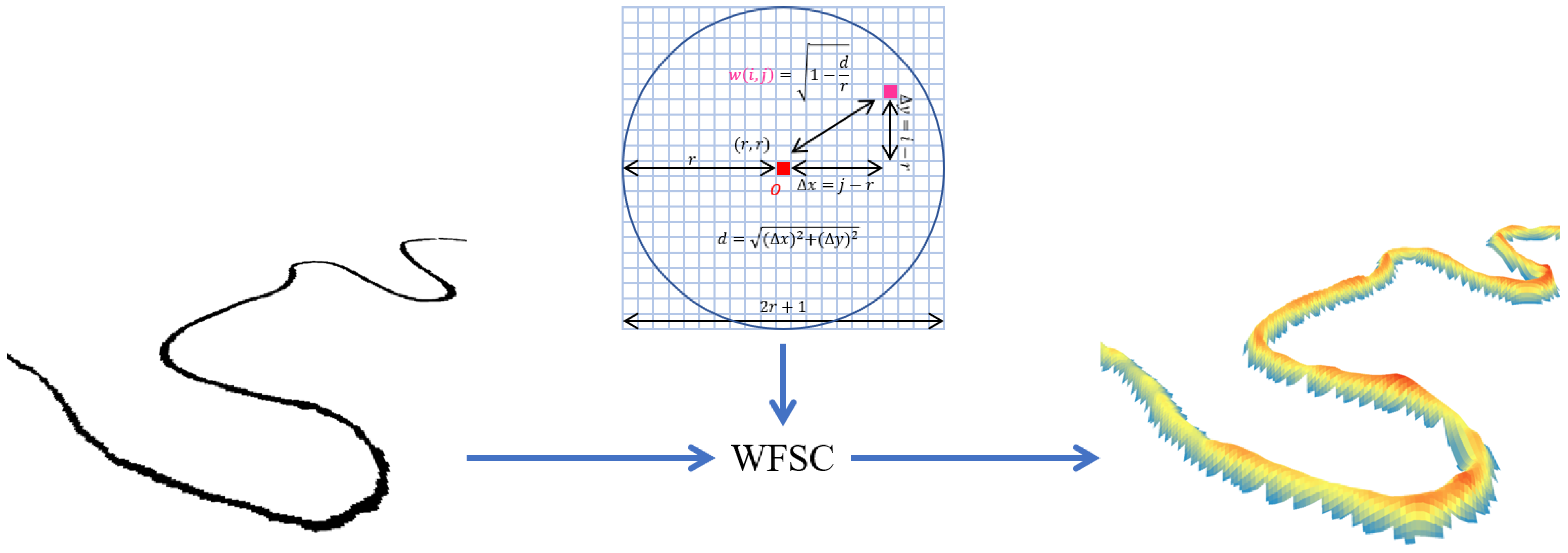
We designed a WFSC to convert the binary lotic habitat image to a magnitude surface (Figure 3). The WFSC is a convolution of a binary image with a weighted focal statistic kernel. For practical use, we designed the weighted focal statistic kernel as a disk-form structure on a square matrix and determined the weights in a distance-inverse format. Each cell on the disk is coded with a weight, and the weight is defined in a radius-based square-rooted form as follows:
where is the weight on the disk; is the Euclidean distance from the cell to the center of the disk; is the row number on the square matrix; and is the column number. The edge length of the square matrix is . The disk has a radius of cells and is centered at on the square matrix. Every cell on the disk is coded with a weight, and other cells are coded with 0. The convolution at on the binary image first extracts an image chip that has the same size as the kernel and is centered at on the image. Then the convolution yields a magnitude value at from:
where is the magnitude value at on the image; is the -th weight on the kernel; and is the conjugate -th pixel value on the image chip. The set contains all the locations on the disk that have a weight.
The convolution at every pixel location on the image object produces a magnitude image (Figure 4b). The convolution returns 0 if the kernel hits nothing on the binary image object. In contrast, the convolution returns a small value when the kernel hits the edge of the linear feature, and it returns the local maximal value when the kernel hits the center of the linear feature. Hence, the magnitude image is a fuzzy representation of the binary image objects, and it is similar to a terrain surface. The centerline of the curvilinear lotic habitat image object on the magnitude image is the same as the ridgeline on the terrain surface. The following steps extract the centerline of the lotic habitat image object as a ridgeline on the terrain surface. The ridgeline on the terrain surface is the divider to separate the surface into two adjacent parts, and the two parts have opposite aspects. Reversely, the line between the regions that have opposite aspects is considered a ridgeline.
The aspect layer is derived from the magnitude surface [49], and the continuous aspect values are reclassified as 8 discrete directions (Figure 4c), as shown in Table 2. The discrete aspect image is filtered using a 5-by-5 majority filter to remove noise [50]. The cell is determined as a ridgeline cell on the filtered discrete aspect image if the aspects of the cell’s west-east neighbors are opposite, or the aspects of the cell’s north-south neighbors are opposite. The opposite aspects are defined as a pair of aspect values whose absolute code difference is larger than 3 and smaller than 5. For instance, Code 5 is opposite to Codes 1, 2, and 8, Code 1 is opposite to Codes 4, 5, and 6. All the ridgeline cells are extracted to form the ridgeline in a raster representation (Figure 4d). A thin algorithm is employed to remove redundant ridgeline cells [51] (Figure 4e).
A tracing algorithm is developed to trace the complete centerlines of the lotic habitat image objects. Since the WFSC is sensitive to the variable width of the lotic habitat image object, the extracted centerline (ridgeline) may be fragmentary. Two thresholds are set to connect the fragmentary ridgelines into long and complete centerlines while eliminating short noisy ridgelines. The first is the gap tolerance and the second is the length of centerline . The thinned image of ridgeline cells is first scanned to find the end nodes of the centerlines. An end node is defined as a ridgeline cell that connects to only one ridgeline cell within its 8 neighbors. A square window with an edge length of is centered on each end node to search for an adjacent end node. If an end node is found within the square window, the spatial gap between these two end nodes is smaller than and they may well be connected on the lotic habitat image object. An imaginary line segment is assigned between the two end nodes and the cells it goes through are designated as ridgeline cells to connect two ridgelines. After filling the gap, the image of the ridgeline cells is scanned again to search for the end nodes. From the first end node, a unique ID is assigned to the ridgeline cell. The tracing starts from the marked ridgeline cell and then marks its adjacent ridgeline cell. The tracing is repeated to reach the other end node of the ridgeline and the total number of ridgeline cells is counted. If the total number of ridgeline cells is larger than the threshold , the marked ridgeline cells are exported as a centerline of the lotic habitat image object. The marked ridgeline cells are reassigned as 0 to avoid duplicated tracing. Otherwise, if the total number of ridgeline cells is smaller than the threshold , the marked ridgeline cells are directly reassigned as 0 without exporting. The unique ID is then updated for the next end node to trace the next centerline. This tracing procedure is repeated until the last end node. All the exported centerlines are converted into line features in a vector format. The steps of the proposed method are developed as a series of tools using Python 3 in ArcGIS Pro.
Three conventional methods were compared with the proposed WFSC method. The first method is the hydrologic delineation of streamline from a DEM. An NED tile is collected from the USGS to fully cover the test site in Figure 1b and the selected lotic habitat image objects. The NED tile is hydrologically enforced by filling the sinks and pits, then the flow directions are calculated using the D8 algorithm [52]. The flow accumulation is derived from the flow direction layer, and the DEM cells with a flow accumulation area larger than 1000 km2 are marked as stream channel cells [16]. A 100-m outward buffer zone is created from the extent of selected lotic habitat image objects to fully contain the hydrologically delineated streamline. The stream channel cells within the buffer zone are exported together to represent the centerlines of the lotic habitat image objects.
The second method for deriving the centerlines of lotic habitat image objects is the grayscale morphological method. The redundantly repeated erosion algorithm in the grayscale morphology finds the skeleton of a linear target on a binary image [53,54]. The same as the proposed method, the selected lotic habitat image objects are first reclassified as a binary image. A 100-time repeated erosion is then applied to the binary image to find the skeletons of the lotic habitat image objects. Since the morphological method is sensitive to the irregular edge of the target, direct erosion may result in trivial artifactual tributaries. To mitigate the influence from the edge, a 100-m (10 pixels) dilation operation is applied to the image objects before the erosion to smooth the edge. The ultimate skeletons of the smoothed lotic habitat image objects are considered their centerlines.
The last employed method is Liu’s phase-coded convolution method [34]. Similar to the proposed WFSC method, the phase-coded convolution can also yield a magnitude surface of the binary image [31]. The convex cells on the magnitude surface are treated as the elements on the surficial ridgelines, and an MCMC algorithm is employed to trace the ridgelines from the convex cells. Again, the traced ridgelines are exported as the centerlines of selected lotic habitat image objects. All the exported centerlines are converted to line features in the vector format for the accuracy assessment.
3.3. Accuracy Assessment
In our framework, the centerlines of river links are essential for structuralizing lotic habitats. Thus, it is crucial to first evaluate the accuracy of the delineated river centerlines. Regarding structuralization, two types of evaluation are necessary: the first is geospatial accuracy and the other is topological consistency. Geospatial accuracy indicates the locational accuracy of the delineation, while topological consistency indicates if the delineated centerlines can properly represent the structure of the lotic habitat.
Liu’s geospatial assessment has already confirmed the adequate accuracy of aquatic habitat image objects delineated from Sentinel-2 images [16]. The centroid displacement and boundary displacement are both well below the spatial resolution of the Sentinel-2 image (10 m), and the areal accuracy is about 93%. These assessments are based on lentic habitat image objects. They can indicate similar adequate accuracy of lotic habitat image objects, like the small locational displacement and boundary displacement. These assessments are not sufficient to evaluate other essential geospatial properties of the delineated lotic habitat image objects. In this study, the other two indices are employed to further evaluate the geospatial accuracy of delineated lotic habitat centerlines [34]. One is length accuracy:
where is the length of the ground truth centerline and is the length of the delineated centerline. The other is centerline average displacement:
where is the displacement area between the delineated centerline and its corresponding ground truth. The second crucial assessment is topological consistency, which indicates whether the delineated centerline can properly represent the structure of the lotic habitat image objects. Because of a lack of quantitative approaches for evaluating the topological consistency of the delineated centerlines, this assessment is simply conducted by visual inspection and interpretation. The number of delineated centerlines is compared with the number of ground truth centerlines to discuss the topological consistency.
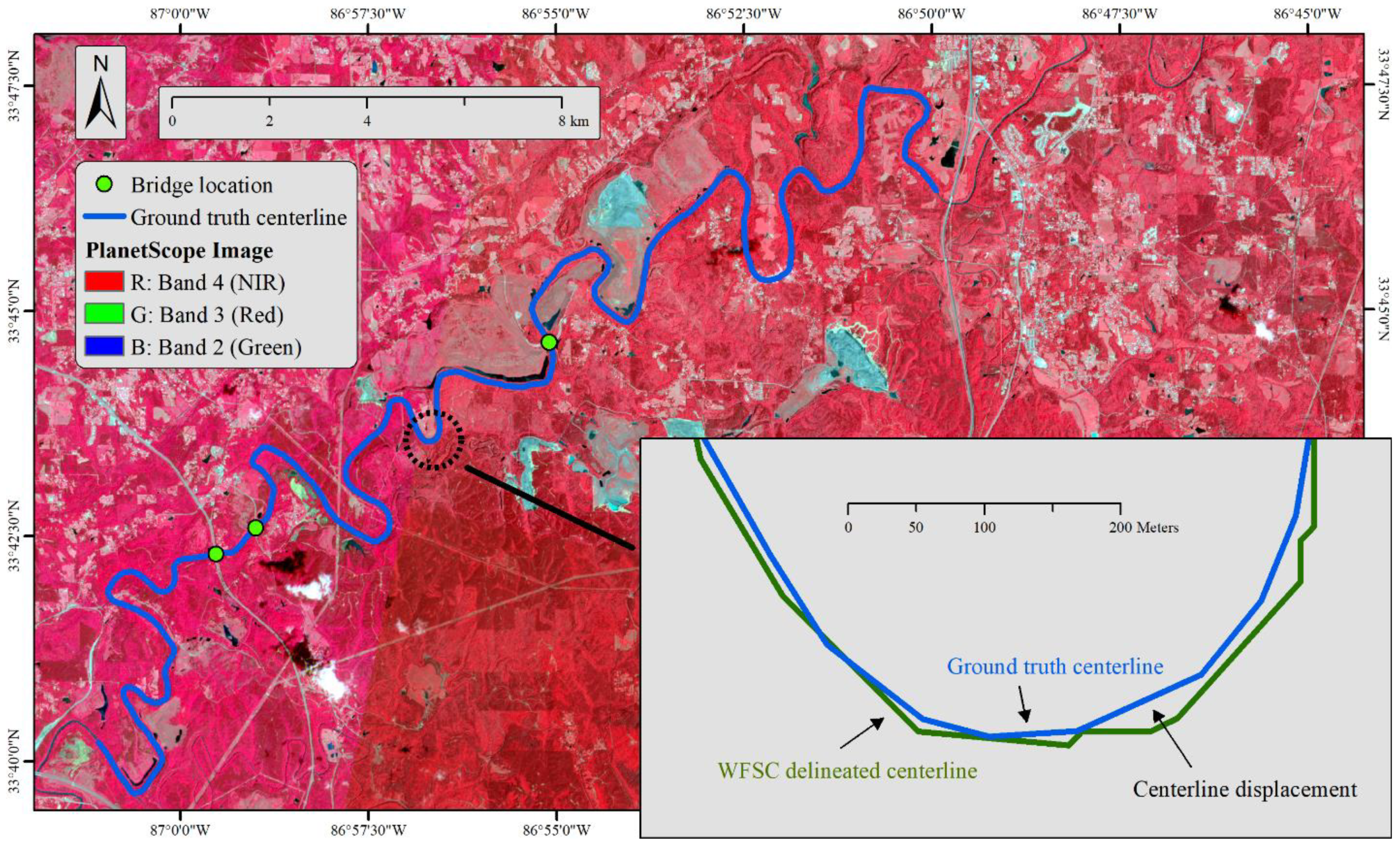
PlanetScope imagery has a high spatial resolution of 3 m and 4 multispectral bands, including blue, green, red, and NIR bands [55]. The high spatial resolution and proper multispectral configuration make it a good data source for interpreting the ground truth of the lotic habitat. In this study, 5 high-resolution PlanetScope images from Planet Labs, Inc. (Figure 5) are visually interpreted to obtain the ground truth of a severely meandering lotic habitat in Figure 1b. These PlanetScope images were captured on 26 April 2019, the capture date is the same as the collected Sentinel-2 image. These images have four spectral bands with 3 m spatial resolution, covering an area of 300 km2 centered on 86°56′ W, 33°44′ N. Since these images have adequate high spatial resolution and proper configuration of spectral bands, the visually interpreted centerline from these images can be used as the ground truth with high confidence and fidelity. The centerline of the lotic habitat is traced from the PlanetScope images in the vector format of the line feature. The , , and are derived from the ground truth and delineated centerlines using a group of spatial analysis tools in ArcGIS 10.5.
3.4. Multi-Level Structuralization of Complicated River Network
The proposed method for extracting river link centerlines relies on convolution to generate a magnitude surface, which is sensitive to the size of the kernel. A small kernel may fully overlap with the lotic habitat image object and result in a saturated magnitude. The assembled saturated magnitude values on the magnitude surface form a flattop. The tracing of a ridgeline automatically stops at the edge of the flattop since no adjacent opposite aspects could be found. The automatic cease of the tracing is particularly meaningful at the joint of a river link and an in-river reservoir. Since a proper kernel size for the river link may well be small to its connected in-river reservoir, saturated magnitude values and the flattop on the magnitude surface then occur within the in-river reservoir. The automatic ceases in the tracing of the surface ridgeline (link centerline) at the entrance and exit of the reservoir achieve the automatic separation of a river link from its adjacent in-river reservoir.
In a much more complicated braided river network (Figure 1c), a universal optimal kernel size does not exist. A multi-level extraction scheme is more suitable to fully structuralize the river network. First, a small kernel with a radius is set to extract the narrowest river links. After convolution, the centerlines of the narrowest river links are delineated with a gap tolerance and a length threshold . In this case, the wider links and ponding water areas will be automatically excluded from the delineation due to the saturation of magnitude values. A buffer zone with the width of is created on both sides of each delineated centerline, and the water surface pixels within the buffer zone are assigned to their nearest centerline and coded with the same unique ID of the centerline. These coded river links are marked as Level-1 river links and the water surface pixels associated with them are excluded from the next round of extraction. The second round of extraction creates a larger kernel with a radius (). The second convolution excludes these pixels in Level-1 river links to generate a magnitude surface. The centerlines are delineated with a gap tolerance and a length threshold . A buffer zone with the width of is created on both sides of each delineated centerline in the second round, and the Level-2 river links and their associated water surface pixels are coded within the buffer. Repeat the procedure until the k-th round to extract the widest river links. The remaining are compact waterbodies. The minimum mapping unit of the delineation in this study is set to 10,000 m2 (1.0 ha). The remaining waterbodies are considered noise and unreliable waterbodies if they are smaller than the minimum unit. These small, remaining waterbodies are merged into their adjacent links. The rest of the remaining water bodies are larger than the minimum mapping unit and are considered particular waterbodies, for instance, in-river reservoirs and bays. Each of them is coded with a unique ID, respectively. The structuralization of the braided river network generates a group of river links at multiple levels, and each river link is coded with a unique ID.
A group of planar geometric attributes is then derivable for each river link, respectively. The structuralized braided river network in the raster format is converted into the vector format in ArcGIS 10.5. The traced centerlines are converted to line features that are stored in a shapefile, and the sets of spatially adjacent pixels coded with each unique ID are converted to polygon features in the other shapefile. The boundaries of polygon features are simplified using the Douglas–Peucker algorithm [56,57]. The simplification tolerance is set to 10 m (1-pixel width on Sentinel-2 image) to smooth saw-toothed edges while maximizing the natural shape of the river links. The line features and polygon features are spatially joined since they share the same ID number. The meander length of a river link is defined as the length of the traced centerline. The straight length of a river link is defined as the straight-line distance between the two endpoints of the river link centerline. The surface area of a river link is defined as the area enclosed by the polygon feature. The average width of a river link is defined as its river link surface area divided by its meander length. The sinuosity index of a link is the meander length divided by its straight length [58,59]. The sinuosity index is a unitless index to describe the planar geometry of the river link. The closer to 1 the sinuosity index is, the link is more like a straight channel; on the contrary, the larger the sinuosity index is, the link has the more apparent meandering shape. These attributes are derived using a group of spatial analysis tools in ArcGIS 10.5.
The abundance pattern of these river links is analyzed based on these derived geospatial attributes. Particularly, the width–abundance pattern is analyzed using the width attribute in the Mobile–Tensaw River Delta in three functions, including a linear function, a power function, and a logarithmic function. These functions use the width of a river link as the independent variable and the number of river links wider than the width as the dependent variable, and they are fitted using the least-squared adjustment approach as follows:
where is the number of river links whose width values are equal to or larger than a threshold width (). The constant coefficients , , and are the decreasing rate in the number of river links corresponding to their width values in the linear function, power function, and logarithmic function, respectively. is the estimated total number of river links with an infinite small width (~0 m) in the linear function. is the estimated total number of river links with a unit width (1 m) in the power function. Similarly, is the estimated total number of river links with a unit width (1 m) in the logarithmic function. The fitting of these functions is based on all the river links derived from the braided river network in the Mobile–Tensaw River Delta (Figure 1c). The coefficient of determination () is used to determine the goodness of fitness.
4. Results and Discussions
4.1. Centerline Extraction and Accuracy Assessment
The initial implementation and accuracy assessment of the proposed WFSC method is conducted for the lotic habitat in Figure 1b. The centerline is delineated using a kernel radius of 70 m (7 pixels) and a gap tolerance of 300 m (30 pixels). The length threshold and the buffer zone width are not applicable in this case. The geospatial accuracy and topological consistency of the WFSC method are compared with the other three conventional methods (Table 3). The lotic habitat in Figure 1b is a long and narrow river channel. It has a meander length of about 48 km and a sinuosity index of 2.33, indicating it is an apparently meandering river link. The severely meandering river link is a tough case to test the performance and robustness of the methods.
The proposed WFSC method shows an overall good performance with high geospatial accuracy and correct topological consistency. The WFSC method, grayscale morphological method, and hydrologic method have achieved equivalent length accuracy and all are about 99%. In contrast, the PCD + MCMC method has only delineated 76% of the total centerline. The PCD method is conventionally used to extract the centerlines of straight linear features like roads [31], while Liu has novelly employed MCMC to enable the PCD method to delineate the centerlines of curvilinear glaciers [34]. However, the MCMC traces the centerline using the trend in the state transition matrix. The trend works well for straight or winding (less meandering) linear features, but it has a high risk to lose the centerlines in the severely sinuous linear features. The WFSC method is similar to the PCD + MCMC method, but the delineation of centerlines is based on the opposite aspects. The experiment indicates that the opposite aspects are more robust than convex pixels in the reliable delineation of centerlines. Regarding the centerline average displacement, the WFSC method, grayscale morphological method, and PCD + MCMC method all are below the spatial resolution of the Sentinel-2 image (10 m), indicating a delineation result with adequate locational accuracy. The hydrologic method has a centerline average displacement of 15.64 m, and the delineated centerline is always close to the edge of the river link rather than the real centerline. The hydrologic method derives accumulated drainage potential from DEM as the lotic habitat centerline. Nowadays, DEM data generally depict only the surface of river links rather than their riverbeds. The flat surface of water results in uncertainties in drainage potential, and the considerable displacement of delineated centerline (streamline) occurs. As a comparison, the other three methods employ computer vision techniques to delineate the centerline of lotic habitats (river links), which minimizes the uncertainties on the flat surface of lotic habitats and promises high locational accuracy.
The WFSC method also shows correct topological information. The test site in Figure 1b is a single river channel with a single long centerline. The delineated lotic habitat is divided into four discrete image objects due to the occlusion of three bridges. The WFSC method and hydrologic method have successfully delineated the centerline as a complete, long, and well-connected linear feature. The hydrologic method achieves the proper topological information by using the drainage potential, which gets rid of the interference from the bridge’s occlusion. The WFSC method mitigates the interference from the bridge’s occlusion by employing a tolerance gap . On the contrary, the PCD + MCMC method depicts the centerline of the lotic habitat as 31 discrete line segments, which is wrong topological information. The grayscale morphological method can also delineate the complete centerline of the lotic habitat, but the topological structure is destroyed by an artifact tributary. The small artifact tributary is caused by an irregular edge of the river link, and an unnecessary skeleton line is then delineated as a centerline. Consequentially, the topological structure of the lotic habitat becomes the confluence of the upstream river link and the artifact tributary into the downstream river link. Although a dilation algorithm has been applied to mitigate the interference from the irregular edge, the unnecessary skeleton line and the artifact tributary are still unavoidable. In summary, the WFSC method has the best overall performance, and it offers better length completeness than the PCD + MCMC method and lower centerline average displacement than the hydrologic method. Further, it also achieves better topological consistency than the PCD + MCMC method and the grayscale morphological method.
The accuracy of the proposed method relies on proper remote sensing data sources. The adequate spatial resolution of public free Sentinel-2 imagery grounds the foundation for the proper structuralization of lotic habitats. A coarser spatial resolution like 30 m on Landsat 8 imagery may miss numerous narrow lotic habitats in the upstream regions. Moreover, the coarser spatial resolution also increases the risk of destroying lotic habitat connectivity by missing the mixed pixels in the middle of river channels. On the contrary, finer spatial resolution is sure to improve the quality of structuralized lotic habitats. However, remote sensing data sources with a finer spatial resolution (e.g., WorldView-2, QuickBird-2, and GeoEye-1) are commercial data. The tremendous cost limits the use of these commercial data on basin-level large-scope investigations. Since lotic habitats are generally spatially sparse with rapid changes, it is not practical to have only small-scope investigations. In summary, Sentinel-2 imagery is currently the most proper data source for the structuralization of lotic habitats on a large scope.
4.2. Parameter Sensitivity and Multi-Level Structuralization
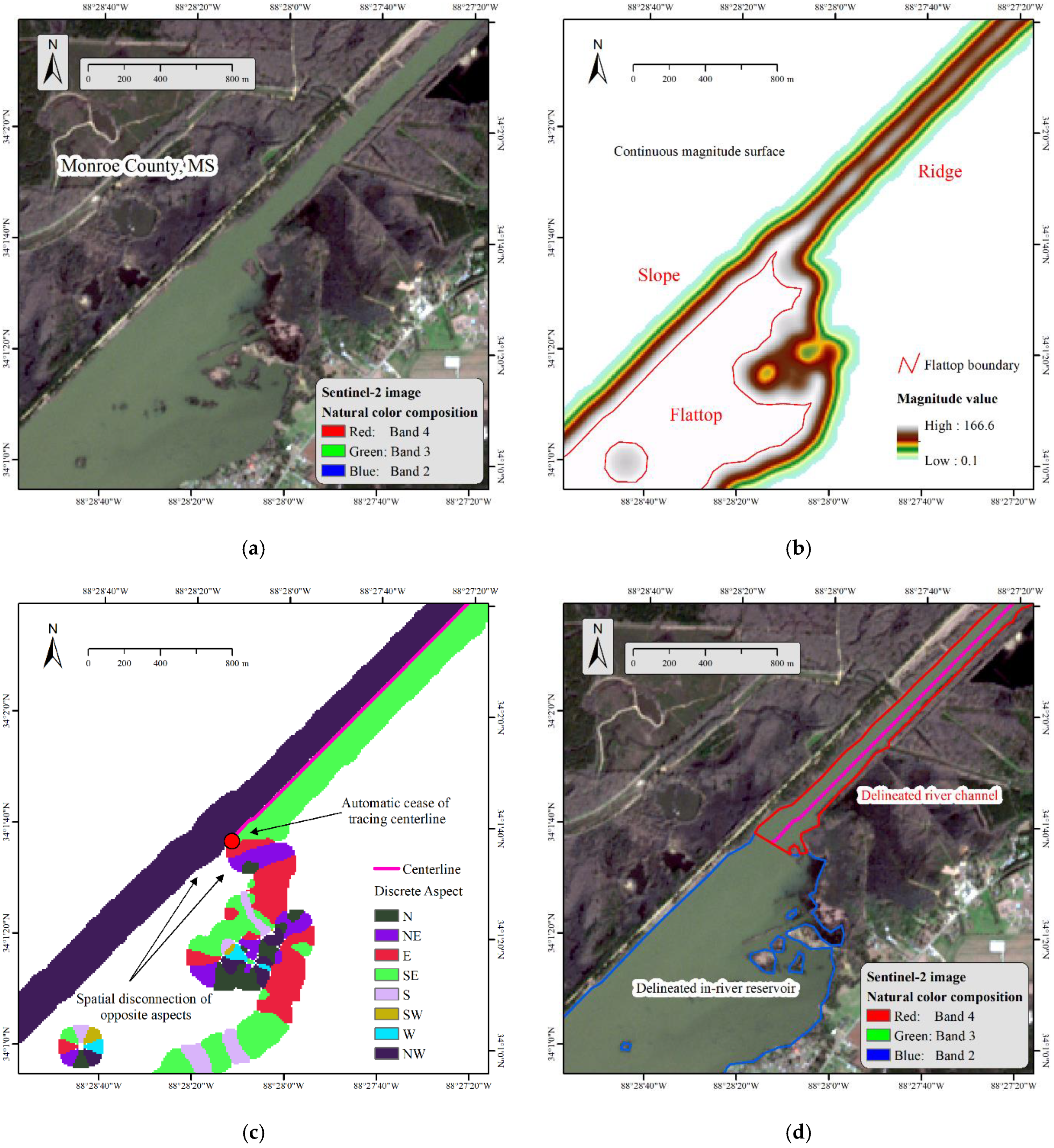
The crucial intermediate variable layer in the WFSC method is the magnitude surface, and the derivation of the magnitude layer is sensitive to the kernel radius . To properly form the magnitude surface of a lotic habitat that has a uniform width, the kernel radius must be slightly larger than the width of the lotic habitat. The slightly larger kernel radius produces a continuous magnitude surface while avoiding the saturated magnitude values and the flattop on the magnitude surface. Theoretically, a much larger kernel radius can yield an equivalent magnitude surface for straight linear features. The centerline in such a case will be represented by the same ridgeline in different magnitude values. However, the practical case of a dense meandering lotic habitat (Figure 6a) indicates that the over-large kernel radius is improper. An overly large kernel may simultaneously overlap with multiple river links in the lotic habitat, which yields a biased or even wrong magnitude surface. On the other hand, the derivation of magnitude surface relies on convolution, the algorithm complexity and the time consumption are . An over-large kernel radius tends to unnecessarily increase the time cost. A case study has been conducted to test the impact of over-large kernel radius (Figure 6b–f). Apparently, the loss of centerline and the time cost both increase exponentially as the kernel radius linearly increases. A proper kernel radius promises the efficient delineation of the lotic habitat centerlines with high length completeness.
Small kernel radius may lead to the full overlap between the kernel and the lotic habitat. Consequentially, the convolution yields saturated magnitude values and a flattop. No adjacent opposite aspects are distributed around the flattop, which leads to the automatic cease of tracing centerlines. An overly small kernel radius is improper since the flattop may lead to fragmentary and topologically incomplete centerlines and even the absolute loss of centerlines. However, the proper usage of the flattop may also achieve the automatic separation of in-river reservoirs from the river links (Figure 7b,c). An in-river reservoir is generally considered a lentic habitat, but it is well connected with multiple river links. Due to the considerable influx and outflux of water, the residence time of water in in-river reservoirs is supposed to be shorter than in isolated lentic habitats (e.g., natural lakes that are isolated from any streams and rivers) but longer than in lotic habitats. This characteristic makes in-river reservoirs a different type of aquatic habitat. The proposed WFSC method enables the automatic separation of in-river reservoirs from their adjacent river links. The WFSC method is applicable and transferable to other study areas, and it enables the investigation of in-river reservoirs on a broader scope. Although beyond the scope of this paper, this topic needs more research.
In a much more complicated real case of a braided river network (Figure 1c), a single optimal kernel radius does not exist. A multi-level structuralization scheme is practical to depict the structure of the braided river network. Through a trial-and-error strategy, the braided river network in the Mobile–Tensaw River Delta is structuralized into 205 river links on 4 levels (Figure 8a–c) using the parameter settings in Table 4. Multiple compact water bodies (e.g., the Grand Bay) are automatically separated from the river links. The river link is defined as a single river channel that has a changeless width, and a very long river channel that has a variable width will be split into multiple river links with uniform widths. The different widths in the channel may lead to a change in flow rate and kinetic energy [60]. The definition of a river link and its delineation in this study is then proper for environmental study purposes. The delineated river links with uniform widths may also have other uniform properties (e.g., flow rate). These properties are essential for the hydrologic modeling of water quality such as the amount of suspended sediment [61].
The proper structuralization of the braided river network in the Mobile–Tensaw River Delta is compared with the hydrologic delineation of the streamline in Figure 8a. The hydrologic method delineates the centerline of the lotic habitat with high length completeness and right topological consistency in a single river channel (Table 3), but it fails in the complicated river network. These mismatches include the wrong upstream channel, the loss of most river links, the erroneous connection of parallel river links, the change in flow course, and so on. On the contrary, the proposed WFSC method and the multi-level structuralization scheme enable the proper structuralization of the braided river network.
4.3. Planar Geometric Attributes Derivation and the Width–Abundance Pattern
The planar geometric attributes of each river link in the braided river network in Figure 1c are numerically derived, respectively. These attributes are summarized in Table 5. The largest and longest river link is the Tensaw River, which has a delineated area of 994.91 ha and a delineated length of 18.83 km. However, the Tensaw River is not the widest river link; its width is 528.45 m, ranking second. The widest river link is a section of the upstream Mobile River that has a width of 646.52 m. The distribution of surface area, meander length, straight length, width (Figure 9), and sinuosity index all are positively skewed, indicating that large, long, wide, and meandering river links are rare. On the contrary, small, short, narrow, and straight river links dominate this delta. Particularly, the mean and median sinuosity index values are 1.121 and 1.274, respectively. The small values indicate that most of the delineated river links are in a straight shape, and severely meandering river links are rare in the Mobile–Tensaw River Delta. The proper structuralization of the river network and the numerical derivation of river link planar geometric attributes are achieved by the proposed WFSC method efficiently and automatically. Lotic habitats generally have a quick evolution and significant changes in riverine shape. Along with the amelioration in the spatial and temporal resolution of remote sensing imagery, the proposed method enables the analysis of riverine morphological changes on a fine river link level, which may promote a broad spectrum of studies.
The width–abundance pattern has been analyzed using a linear function, a power function, and a logarithmic function. The least-square fitting indicates that the width–abundance pattern of river links matches a logarithmic function the best, with an of 0.977 (Table 6). The fitted logarithmic function also well estimates the total number of river links in the Mobile–Tensaw River Delta. The estimated river link amount is 225 while the ground truth is 205. On the contrary, the linear function severely underestimates the abundance of river links, and the power function severely overestimates the abundance of river links. The result shows a logarithmic decreasing rate of river link abundance with an increasing river link width, which indicates a possible width–abundance logarithmic law.
The abundance pattern, especially the size–abundance pattern of lentic habitats, has been intensively discussed for several decades using multiple approaches on various scales [16,62,63,64]. A similar analysis is quite limited for lotic habitats because the delineation and proper structuralization of lotic habitats are challenging. This study has proposed a robust method to properly structuralize the complicated braided river network automatically. The braided river network is structuralized on a link level with the attributes numerically derived, respectively. These link-level attributes provide a large volume of measurements to inspect the width–abundance pattern. The proposed method is easily transferable and applicable to the complicated lotic habitats in other deltas and braided river networks. For instance, the braided river network in the downstream Amazon River, the Pearl River Delta, and the Ganges Delta. Thus, the proposed WFSC method may be used to uncover and verify a width–abundance law of the global lotic habitats.
5. Conclusions
A novel robust method has been developed in this study to properly structuralize complicated lotic habitats using Sentinel-2 imagery and weighted focal statistic convolution (WFSC), and it was successfully applied to a braided river network in the MRB. The new generation of Sentinel-2 satellite sensors can provide freely available multispectral imagery with sufficient spatial resolution and proper spectral configuration for delineating lotic habitats at a large scale, which provides a solid foundation for the proper structuralization of lotic habitats through remote sensing approaches. The further integration of GIS and computer vision techniques enables the proper structuralization of complicated lotic habitats with adequate spatial accuracy and correct topological consistency. The structure of complicated lotic habitats is then properly delineated on the river link level. Accuracy assessments indicate that our proposed method can well represent the actual structure of an extremely meandering lotic habitat, with correct topological information and small centerline displacement that is lower than the spatial resolution of Sentinel-2 imagery.
With properly structuralized lotic habitats, essential planar attributes of lotic habitats are automatically and numerically derivable for single river links. For instance, the width and the sinuosity of rivers with hundreds of channels are difficult to obtain on a large spatial scale, but they are easy to derive from the properly structuralized river link image objects. These essential planar attributes for each individual river link can quantitatively support a broad spectrum of environmental studies. Meanwhile, a large number of measurements enables us to uncover the hidden patterns of complicated river networks. A striking width–abundance logarithmic pattern of the braided river networks was observed in our study area, indicating a promising logarithmic law in lotic habitat abundance.
The developed WFSC method can be easily applied and transferred to other study areas on a broader scope. Several possible following works are highlighted here. The developed method can be applied to other complicated braided river networks to verify the promising width–abundance logarithmic law. With time series of Sentinel-2 images, the developed method can be used to quantitatively inspect the morphological evolution of the river links through a range of numerical attributes.
Author Contributions
Conceptualization, methodology, software, validation, formal analysis, investigation, resources, data curation, and visualization, Y.L.; writing—original draft preparation, Y.L. and M.-P.K.; writing—review and editing, Y.L. and M.-P.K. All authors have read and agreed to the published version of the manuscript.
Data Availability Statement
The Sentinel-2 data that support the findings of this study are freely available from ESA Copernicus Open Access Hub (https://scihub.copernicus.eu/dhus/#/home). The NED data are freely available from the USGS National Map (https://apps.nationalmap.gov/downloader/#/). The PlanetScope data are collected from Planet Labs, Inc. (https://www.planet.com/explorer/) using an Education and Research (ER) license.
Conflicts of Interest
The authors declare no conflict of interest.
Code Availability Statement
The code and programs developed in the study will be provided upon reasonable request.
Abbreviations and Notations
GIS—Geographic Information System, WFSC—Weighted Focal Statistic Convolution, GEOBIA—Geographic Object-based Image Analysis, HAB—Harmful Algal Bloom, PCD—Phase-Coded Disk, MCMC—Markov chain Monte Carlo, MRB—Mobile River Basin, ESA—European Space Agency, NED—National Elevation Dataset, USGS—United States Geological Survey, MSI—Multispectral Instrument, NIR—near-infrared, SWIR—short-wave infrared, TOA—Top-Of-Atmosphere, DEM—Digital Elevation Model, ISODATA—Iterative Self-Organizing Data Analysis Technique, GL—ground truth length, DL—delineated length, DA—displacement area, —kernel disk radius, —gap tolerance, —centerline length threshold, —buffer zone width, —round number of multi-level structuralization, —threshold width of the lotic habitat, —the number of river links whose width values are equal to or larger than , —coefficient of determination.
References
- Fisher, W.L.; Bozek, M.A.; Vokoun, J.C.; Jacobson, R.B. Freshwater aquatic habitat measurements. In Fisheries Techniques, 3rd ed.; American Fisheries Society: Bethesda, MD, USA, 2012; pp. 101–161. [Google Scholar]
- Bain, M.B.; Stevenson, N.J. Aquatic Habitat Assessment; Asian Fisheries Society: Bethesda, MD, USA, 1999. [Google Scholar]
- Jones, A.E.; Hodges, B.R.; McClelland, J.W.; Hardison, A.K.; Moffett, K.B. Residence-time-based classification of surface water systems. Water Resour. Res. 2017, 53, 5567–5584. [Google Scholar] [CrossRef]
- Mulder, T.; Syvitski, J.P.; Skene, K.I. Modeling of erosion and deposition by turbidity currents generated at river mouths. J. Sediment. Res. 1998, 68, 124–137. [Google Scholar] [CrossRef]
- Hizzett, J.L.; Hughes Clarke, J.E.; Sumner, E.J.; Cartigny, M.; Talling, P.; Clare, M. Which triggers produce the most erosive, frequent, and longest runout turbidity currents on deltas? Geophys. Res. Lett. 2018, 45, 855–863. [Google Scholar] [CrossRef] [Green Version]
- Lane, S.N.; Westaway, R.M.; Murray Hicks, D. Estimation of erosion and deposition volumes in a large, gravel-bed, braided river using synoptic remote sensing. Earth Surf. Process. Landf. J. Br. Geomorphol. Res. Group 2003, 28, 249–271. [Google Scholar] [CrossRef]
- Milan, D.J.; Heritage, G.L.; Hetherington, D. Application of a 3D laser scanner in the assessment of erosion and deposition volumes and channel change in a proglacial river. Earth Surf. Process. Landf. J. Br. Geomorphol. Res. Group 2007, 32, 1657–1674. [Google Scholar] [CrossRef]
- Montgomery, D.R. Valley formation by fluvial and glacial erosion. Geology 2002, 30, 1047–1050. [Google Scholar] [CrossRef]
- Constantine, J.A.; Dunne, T. Meander cutoff and the controls on the production of oxbow lakes. Geology 2008, 36, 23–26. [Google Scholar] [CrossRef]
- Seybold, H.; Andrade, J.S.; Herrmann, H.J. Modeling river delta formation. Proc. Natl. Acad. Sci. USA 2007, 104, 16804–16809. [Google Scholar] [CrossRef] [Green Version]
- Strokal, M.; Ma, L.; Bai, Z.; Luan, S.; Kroeze, C.; Oenema, O.; Velthof, G.; Zhang, F. Alarming nutrient pollution of Chinese rivers as a result of agricultural transitions. Environ. Res. Lett. 2016, 11, 024014. [Google Scholar] [CrossRef] [Green Version]
- He, R.; Yang, X.; Gassman, P.W.; Wang, G.; Yu, C. Spatiotemporal characterization of nutrient pollution source compositions in the Xiaohong River Basin, China. Ecol. Indic. 2019, 107, 105676. [Google Scholar] [CrossRef]
- Kiedrzyńska, E.; Kiedrzyński, M.; Urbaniak, M.; Magnuszewski, A.; Skłodowski, M.; Wyrwicka, A.; Zalewski, M. Point sources of nutrient pollution in the lowland river catchment in the context of the Baltic Sea eutrophication. Ecol. Eng. 2014, 70, 337–348. [Google Scholar] [CrossRef]
- Dalu, T.; Wasserman, R.J.; Magoro, M.L.; Froneman, P.W.; Weyl, O.L. River nutrient water and sediment measurements inform on nutrient retention, with implications for eutrophication. Sci. Total Environ. 2019, 684, 296–302. [Google Scholar] [CrossRef] [PubMed]
- Amin, M.N.; Kroeze, C.; Strokal, M. Human waste: An underestimated source of nutrient pollution in coastal seas of Bangladesh, India and Pakistan. Mar. Pollut. Bull. 2017, 118, 131–140. [Google Scholar] [CrossRef]
- Liu, Y.; Liu, H.; Wang, L.; Xu, M.; Cohen, S.; Liu, K. Derivation of spatially detailed lentic habitat map and inventory at a basin scale by integrating multispectral Sentinel-2 satellite imagery and USGS Digital Elevation Models. J. Hydrol. 2021, 603, 126876. [Google Scholar] [CrossRef]
- Phiri, D.; Simwanda, M.; Salekin, S.; Nyirenda, V.R.; Murayama, Y.; Ranagalage, M. Sentinel-2 data for land cover/use mapping: A review. Remote Sens. 2020, 12, 2291. [Google Scholar] [CrossRef]
- Najafzadeh, M.; Homaei, F.; Farhadi, H. Reliability assessment of water quality index based on guidelines of national sanitation foundation in natural streams: Integration of remote sensing and data-driven models. Artif. Intell. Rev. 2021, 54, 4619–4651. [Google Scholar] [CrossRef]
- Wang, L.; Xu, M.; Liu, Y.; Liu, H.; Beck, R.; Reif, M.; Emery, E.; Young, J.; Wu, Q. Mapping freshwater chlorophyll-a concentrations at a regional scale integrating multi-sensor satellite observations with Google earth engine. Remote Sens. 2020, 12, 3278. [Google Scholar] [CrossRef]
- Tarboton, D.G. Terrain analysis using digital elevation models in hydrology. In Proceedings of the 23rd ESRI International Users Conference, San Diego, CA, USA, 7–11 July 2003. [Google Scholar]
- Moore, I.D.; Grayson, R.; Ladson, A. Digital terrain modelling: A review of hydrological, geomorphological, and biological applications. Hydrol. Process. 1991, 5, 3–30. [Google Scholar] [CrossRef]
- Jasiewicz, J.; Metz, M. A new GRASS GIS toolkit for Hortonian analysis of drainage networks. Comput. Geosci. 2011, 37, 1162–1173. [Google Scholar] [CrossRef]
- Tarboton, D.G. Terrain Analysis Using Digital Elevation Models (TauDEM); Utah State University: Logan, UT, USA, 2005; Volume 3012, p. 2018. [Google Scholar]
- Strahler, A.N. Quantitative analysis of watershed geomorphology. Eos Trans. Am. Geophys. Union 1957, 38, 913–920. [Google Scholar] [CrossRef]
- Shreve, R.L. Statistical law of stream numbers. J. Geol. 1966, 74, 17–37. [Google Scholar] [CrossRef]
- Ngoc, D.D.; Loisel, H.; Jamet, C.; Vantrepotte, V.; Duforêt-Gaurier, L.; Minh, C.D.; Mangin, A. Coastal and inland water pixels extraction algorithm (WiPE) from spectral shape analysis and HSV transformation applied to Landsat 8 OLI and Sentinel-2 MSI. Remote Sens. Environ. 2019, 223, 208–228. [Google Scholar] [CrossRef]
- Soille, P. Morphological Image Analysis: Principles and Applications; Springer Science & Business Media: Berlin, Germany, 2013. [Google Scholar]
- Bibiloni, P.; González-Hidalgo, M.; Massanet, S. General-purpose curvilinear object detection with fuzzy mathematical morphology. Appl. Soft Comput. 2017, 60, 655–669. [Google Scholar] [CrossRef]
- Soille, P.; Pesaresi, M. Advances in mathematical morphology applied to geoscience and remote sensing. IEEE Trans. Geosci. Remote Sens. 2002, 40, 2042–2055. [Google Scholar] [CrossRef]
- Clode, S.P.; Zelniker, E.E.; Kootsookos, P.J.; Clarkson, I.V.L. A phase coded disk approach to thick curvilinear line detection. In Proceedings of the 2004 12th European Signal Processing Conference, Vienna, Austria, 6–10 September 2004; pp. 1147–1150. [Google Scholar]
- Clode, S.; Rottensteiner, F.; Kootsookos, P.; Zelniker, E. Detection and vectorization of roads from lidar data. Photogramm. Eng. Remote Sens. 2007, 73, 517–535. [Google Scholar] [CrossRef] [Green Version]
- Hu, X.; Li, Y.; Shan, J.; Zhang, J.; Zhang, Y. Road centerline extraction in complex urban scenes from LiDAR data based on multiple features. IEEE Trans. Geosci. Remote Sens. 2014, 52, 7448–7456. [Google Scholar]
- Clode, S.; Kootsookos, P.J.; Rottensteiner, F. The Automatic Extraction of Roads from LIDAR Data; ISPRS: Istanbul, Turkey, 2004. [Google Scholar]
- Liu, Y. Automatically Structuralize the Curvilinear Glacier Using Phase-coded Convolution. IEEE Geosci. Remote Sens. Lett. 2021, 19, 1–5. [Google Scholar] [CrossRef]
- Beshr, A.M.; Mohamed, A.K.; ElGalladi, A.; Gaber, A.; El-Baz, F. Structural characteristics of the Qena Bend of the Egyptian Nile River, using remote-sensing and geophysics. Egypt. J. Remote Sens. Space Sci. 2021, 24, 999–1011. [Google Scholar] [CrossRef]
- Nones, M. Remote sensing and GIS techniques to monitor morphological changes along the middle-lower Vistula river, Poland. Int. J. River Basin Manag. 2021, 19, 345–357. [Google Scholar] [CrossRef]
- Boothroyd, R.J.; Nones, M.; Guerrero, M. Deriving planform morphology and vegetation coverage from remote sensing to support river management applications. Front. Environ. Sci. 2021, 9, 657354. [Google Scholar] [CrossRef]
- McPherson, A.K.; Moreland, R.S.; Atkins, J.B. Occurrence and Distribution of Nutrients, Suspended Sediment, and Pesticides in the Mobile River Basin, Alabama, Georgia, Mississippi, and Tennessee, 1999–2001; US Department of the Interior: Washington, DC, USA; US Geological Survey: Montgomery, AL, USA, 2003.
- Atkins, J.B.; Zappia, H.; Robinson, J.L.; McPherson, A.K.; Moreland, R.S.; Harned, D.A.; Johnston, B.F.; Harvill, J.S. Water Quality in the Mobile River Basin, Alabama, Georgia, and Mississippi, and Tennessee, 1999–2001; US Geological Survey: Montgomery, AL, USA, 2004.
- Liu, A.; Ming, J.; Ankumah, R.O. Nitrate contamination in private wells in rural Alabama, United States. Sci. Total Environ. 2005, 346, 112–120. [Google Scholar] [CrossRef] [PubMed]
- Schroeder, W.W.; Dinnel, S.P.; Wiseman, W.J. Salinity stratification in a river-dominated estuary. Estuaries 1990, 13, 145–154. [Google Scholar] [CrossRef]
- Liu, Y.; Kwan, M.-P.; Wu, Z. Visualizing and quantifying the spatiotemporal expansion of the Blue Lentic Belt in Alabama and Mississippi. Water Res. 2022, 217, 118444. [Google Scholar] [CrossRef] [PubMed]
- Frampton, W.J.; Dash, J.; Watmough, G.; Milton, E.J. Evaluating the capabilities of Sentinel-2 for quantitative estimation of biophysical variables in vegetation. ISPRS J. Photogramm. Remote Sens. 2013, 82, 83–92. [Google Scholar] [CrossRef] [Green Version]
- Drusch, M.; Del Bello, U.; Carlier, S.; Colin, O.; Fernandez, V.; Gascon, F.; Hoersch, B.; Isola, C.; Laberinti, P.; Martimort, P. Sentinel-2: ESA’s optical high-resolution mission for GMES operational services. Remote Sens. Environ. 2012, 120, 25–36. [Google Scholar] [CrossRef]
- Dubes, R.; Jain, A.K. Clustering techniques: The user’s dilemma. Pattern Recognit. 1976, 8, 247–260. [Google Scholar] [CrossRef]
- Tou, J.T.; Gonzalez, R.C. Pattern Recognition Principles; Addison-Wesley Publishing: Boston, MA, USA, 1974. [Google Scholar]
- Sonka, M.; Hlavac, V.; Boyle, R. Image Processing, Analysis, and Machine Vision; Springer: New York, NY, USA, 2014. [Google Scholar]
- Bachelot, B.; Uriarte, M.; Zimmerman, J.K.; Thompson, J.; Leff, J.W.; Asiaii, A.; Koshner, J.; McGuire, K. Long-lasting effects of land use history on soil fungal communities in second-growth tropical rain forests. Ecol. Appl. 2016, 26, 1881–1895. [Google Scholar] [CrossRef] [Green Version]
- Burrough, P.A.; McDonnell, R.A.; Lloyd, C.D. Principles of Geographical Information Systems; Oxford University Press: Oxford, UK, 2015. [Google Scholar]
- Stuckens, J.; Coppin, P.; Bauer, M. Integrating contextual information with per-pixel classification for improved land cover classification. Remote Sens. Environ. 2000, 71, 282–296. [Google Scholar] [CrossRef]
- Zhan, C. A hybrid line thinning approach. In Proceedings of the Autocarto-Conference, Minneapolis, MN, USA, 30 October–1 November 1993; p. 396. [Google Scholar]
- O’Callaghan, J.F.; Mark, D.M. The extraction of drainage networks from digital elevation data. Comput. Vis. Graph. Image Process. 1984, 28, 323–344. [Google Scholar] [CrossRef]
- Maragos, P.; Schafer, R. Morphological skeleton representation and coding of binary images. IEEE Trans. Acoust. Speech Signal Process. 1986, 34, 1228–1244. [Google Scholar] [CrossRef]
- Su, Y.; Zhong, Y.; Zhu, Q.; Zhao, J. Urban scene understanding based on semantic and socioeconomic features: From high-resolution remote sensing imagery to multi-source geographic datasets. ISPRS J. Photogramm. Remote Sens. 2021, 179, 50–65. [Google Scholar] [CrossRef]
- Planet. Planet Application Program Interface: In Space for Life on Earth; Planet: San Francisco, CA, USA, 2017; Volume 2017, p. 40. [Google Scholar]
- Saalfeld, A. Topologically consistent line simplification with the Douglas-Peucker algorithm. Cartogr. Geogr. Inf. Sci. 1999, 26, 7–18. [Google Scholar] [CrossRef]
- Douglas, D.H.; Peucker, T.K. Algorithms for the reduction of the number of points required to represent a digitized line or its caricature. Cartogr. Int. J. Geogr. Inf. Geovis. 1973, 10, 112–122. [Google Scholar] [CrossRef] [Green Version]
- Ghosh, S.; Mistri, B. Hydrogeomorphic significance of sinuosity index in relation to river instability: A case study of Damodar River, West Bengal, India. Int. J. Adv. Earth Sci. 2012, 1, 49–57. [Google Scholar]
- Mueller, J.E. An introduction to the hydraulic and topographic sinuosity indexes. Ann. Assoc. Am. Geogr. 1968, 58, 371–385. [Google Scholar] [CrossRef]
- Zhou, S.; Wang, X.; Yang, Q.; Huang, Z. Numerical and experimental study the effects of river width changes on flow characteristics in a flume. In Proceedings of the IOP Conference Series: Earth and Environmental Science, Guangzhou, China, 8–10 March 2019; p. 042004. [Google Scholar]
- Juez, C.; Hassan, M.A.; Franca, M.J. The origin of fine sediment determines the observations of suspended sediment fluxes under unsteady flow conditions. Water Resour. Res. 2018, 54, 5654–5669. [Google Scholar] [CrossRef]
- Downing, J.A.; Prairie, Y.; Cole, J.; Duarte, C.; Tranvik, L.; Striegl, R.G.; McDowell, W.; Kortelainen, P.; Caraco, N.; Melack, J. The global abundance and size distribution of lakes, ponds, and impoundments. Limnol. Oceanogr. 2006, 51, 2388–2397. [Google Scholar] [CrossRef] [Green Version]
- Verpoorter, C.; Kutser, T.; Seekell, D.A.; Tranvik, L.J. A global inventory of lakes based on high-resolution satellite imagery. Geophys. Res. Lett. 2014, 41, 6396–6402. [Google Scholar] [CrossRef]
- Seekell, D.A.; Pace, M.L.; Tranvik, L.J.; Verpoorter, C. A fractal-based approach to lake size-distributions. Geophys. Res. Lett. 2013, 40, 517–521. [Google Scholar] [CrossRef]
Figure 1.
The geographic settings of the MRB (d) and inside lotic habitats: (a) parallel river channels and in-river reservoirs (3/19/2019); (b) meandering river channel (4/26/2019); and (c) braided river network (3/19/2019). Sentinel-2 image data are from ESA, DEM data are from USGS. Waterbodies are highlighted in sapphirine.

Figure 2.
Flowchart of the structuralization method using WFSC.

Figure 3.
An example of the weighted focal statistic filter and the WFSC. The WFSC converts the lotic habitat image object in the binary raster representation into a continuous magnitude surface, and the centerline of the lotic habitat image object/link corresponds well to the ridgeline on the magnitude surface.

Figure 4.
An illustration of the proposed method: (a) The lotic habitat image object in the raster format; (b) the magnitude surface generated from the WFSC; (c) the derived discrete aspect image; (d) the traced centerline from opposite aspect codes; (e) the thinned centerline in the raster format; and (f) the delineated centerline in the vector format.

Figure 5.
The spatial accuracy assessment of the centerline in the meandering lotic habitat.

Figure 6.
The impacts of over-large kernel size. (a) A complicated lotic habitat for experiment, and the magnitude surface generated from the kernel radius (b) r = 5, (c) r = 15, (d) r = 25, (e) r = 35 and (f) r = 45. As the kernel size linearly increases, the loss of the centerline and the time cost both increase exponentially.

Figure 7.
The function of small kernel size and the automatic separation of the river channel and in-river reservoir: (a) a reservoir connected with a channel; (b) the magnitude surface and a flattop of saturated magnitude values; (c) the automatic cease of tracing centerline due to the spatial disconnection of opposite aspects; and (d) the separation of the river channel and in-river reservoir using the delineated river channel centerline.

Figure 8.
The structuralization of the braided river network in the Mobile–Tensaw River Delta (Figure 1c) using a multi-level scheme. The single lotic habitat image object has been properly structuralized into 205 river links on 4 levels and 21 non-link waterbodies.
Figure 8.
The structuralization of the braided river network in the Mobile–Tensaw River Delta (Figure 1c) using a multi-level scheme. The single lotic habitat image object has been properly structuralized into 205 river links on 4 levels and 21 non-link waterbodies.

Figure 9.
The width–abundance pattern of the river links in the Mobile–Tensaw River Delta.


Table 1.
Dataset summary.
| Task | Data Source | Spatial Resolution | Spectral Configuration | Capture Date | Coverage |
|---|---|---|---|---|---|
| Meandering river channel delineation | Sentinel-2, ESA | 10 m | R, G, B, and NIR | 4/26/2019 | 300 km2 centered on 86°56′W, 33°44′N |
| Braided river network delineation | Sentinel-2, ESA | 10 m | R, G, B, and NIR | 3/19/2019 | The Mobile–Tensaw River Delta |
| Meandering river channel ground truth | PlanetScope | 3 m | R, G, B, and NIR | 4/26/2019 | 300 km2 centered on 86°56′W, 33°44′N |
| Hydrologic reference | NED, USGS | 10 m | - | - | The MRB |
Table 2.
The reclassification scheme of aspects.
| Northwest Aspect: 292.5°~337.5° Code: 8 | North Aspect: 337.5°~360°, 0°~22.5° Code: 1 | Northeast Aspect: 22.5°~67.5° Code: 2 |
| West Aspect: 247.5°~292.5° Code: 7 | No Data | East Aspect: 67.5°~112.5° Code: 3 |
| Southwest Aspect: 202.5°~247.5° Code: 6 | South Aspect: 157.5°~202.5° Code: 5 | Southeast Aspect: 112.5°~157.5° Code: 4 |
Table 3.
The accuracy of centerline delineation using the four methods in this study.
| Centerline Length (km) | Length Accuracy (%) | Centerline Average Displacement (m) | Topological Consistency (Number of Links) | |
|---|---|---|---|---|
| Ground truth | 47.54 | - | - | 1 |
| Hydrologic method | 47.98 | 99.09 | 15.64 | 1 |
| Morphological method | 48.10 | 98.83 | 9.87 | 3 |
| PCD + MCMC | 36.31 | 76.38 | 7.60 | 31 |
| WFSC + Aspects | 48.01 | 99.01 | 9.58 | 1 |
Table 4.
The multi-level parameter settings in the structuralization of the braided river network in the Mobile–Tensaw River Delta.
Table 4.
The multi-level parameter settings in the structuralization of the braided river network in the Mobile–Tensaw River Delta.
| Level k | Kernel Radius rk | Gap Tolerance gk | Length Threshold * lk | Buffer Zone Width bk |
|---|---|---|---|---|
| 1 | 7 | 10 | 50 | 14 |
| 2 | 10 | 20 | 100 | 20 |
| 3 | 20 | 30 | 150 | 40 |
| 4 | 35 | 100 | 150 | 70 |
* unit in pixels, the pixel size on Sentinel-2 imagery is 10 m.
Table 5.
The planform geometric attributes of delineated links.
| Surface Area (ha, 104 m2) | Meander Length (km) | Straight Length (km) | Width (m) | Sinuosity Index | |
|---|---|---|---|---|---|
| Min | 1.990 | 0.532 | 0.375 | 24.338 | 1.000 |
| Median | 13.800 | 1.318 | 1.140 | 101.953 | 1.121 |
| Mean | 34.596 | 2.186 | 1.684 | 125.353 | 1.274 |
| Max | 994.910 | 18.827 | 17.374 | 646.516 | 4.622 |
| Std. | 83.568 | 2.442 | 1.815 | 94.599 | 0.444 |
Table 6.
The regression results of the width–abundance pattern.
| Function | Equation | Estimated Link Abundance with W = 24.34 m * | |
|---|---|---|---|
| Linear | 0.742 | 158 | |
| Power | 0.860 | 482 | |
| Logarithmic | 0.977 | 225 | |
| Ground truth | - | - | 205 |
* W = 24.34 m is the smallest link width in the Mobile–Tensaw River Delta, the corresponding link abundance is the estimated total number of links in the Mobile–Tensaw River Delta.
Publisher’s Note: MDPI stays neutral with regard to jurisdictional claims in published maps and institutional affiliations. |
© 2022 by the authors. Licensee MDPI, Basel, Switzerland. This article is an open access article distributed under the terms and conditions of the Creative Commons Attribution (CC BY) license (https://creativecommons.org/licenses/by/4.0/).
Share and Cite
MDPI and ACS Style
Liu, Y.; Kwan, M.-P. Structuralization of Complicated Lotic Habitats Using Sentinel-2 Imagery and Weighted Focal Statistic Convolution. Hydrology 2022, 9, 195. https://doi.org/10.3390/hydrology9110195
AMA Style
Liu Y, Kwan M-P. Structuralization of Complicated Lotic Habitats Using Sentinel-2 Imagery and Weighted Focal Statistic Convolution. Hydrology. 2022; 9(11):195. https://doi.org/10.3390/hydrology9110195
Chicago/Turabian StyleLiu, Yang, and Mei-Po Kwan. 2022. "Structuralization of Complicated Lotic Habitats Using Sentinel-2 Imagery and Weighted Focal Statistic Convolution" Hydrology 9, no. 11: 195. https://doi.org/10.3390/hydrology9110195
Note that from the first issue of 2016, this journal uses article numbers instead of page numbers. See further details here.