1. Introduction
The Tempisque river basin provides water for human consumption, as well as for productive activities (irrigation, aquaculture, fishing, and electricity generation) and tourism, also fulfills ecological functions such as groundwater recharge and wildlife habitat [
1]; however, the development of the region has caused an uncontrolled increase in the use of surface and groundwater, which has affected the natural behavior of the river, threatening the social, economic and ecological integrity of the region, especially during the dry season [
2].
In contrast, the principles of integrated water resource management are presented to balance water availability with water use, from which the concept of environmental flow is derived as a tool to maintain adequate conditions for the benefit of ecosystem health. In Costa Rica, several investigations have been carried out testing different methodologies, such as the study conducted in the Birrís River sub-basin using a hydrological methodology [
3], the Pejibaye River sub-basin using a hydrobiological methodology [
4], and the Tempisque river basin using a holistic methodology.
Through hydraulic modeling, it is possible to estimate flow velocities and depths and relate the flow rate to the habitat index of certain organisms [
5]. With the use of numerical models, it is possible to run hydraulic simulations with a high level of accuracy in river sections, for this, it is essential to know the available information about the riverbed, such as topography and hydraulic conditions; or obtain them through field visits, to feed and calibrate the numerical model; enabling a meso-habitat scale analysis, which is more realistic and appropriate to assess the availability of physical habitat for biota [
6]. Therefore calibration is key to more accurately representing the real behavior of the channel, as well as to obtaining reliable results [
7].
As far as natural channel models are concerned, calibration is an iterative process in which the roughness coefficient of the channel is varied to reduce the difference between the observed data and the simulated data [
8]. Powell et al. [
9] emphasize that in hydraulic models, it is important that the flow resistance is properly represented in natural channels such as streams and rivers and obtain a detailed description of the flow, especially in rivers where the spatial distribution varies along the section [
10].
Through this study, calibrated hydraulic models were developed for the Ahogados and Tempisquito rivers belonging to the Tempisque river basin, and the process allowed the correction of the empirical equations known as “Strickler-type” of various authors for the calculation of the Manning’s roughness coefficient for conditions of the North Pacific of Costa Rica, through the use of mathematical models and verification with morphological parameters measured in the field. These products will be a resource for further hydrometric and habitat simulation applications to determine the environmental flow of the watershed and contribute to water conservation and protection. The calibrated hydraulic models proved the importance of using comprehensive and detailed field data to successfully simulate the behavior of hydraulic parameters such as velocity and depth in natural channels (fundamental for habitat analysis), as well as to allow a better analysis of the morphological behavior of the channels understudy, which made possible the adjustment of the empirical equations that could be used for future studies in rivers of the northern pacific region of the country or rivers with similar characteristics to those studied in this paper.
2. Materials and Methods
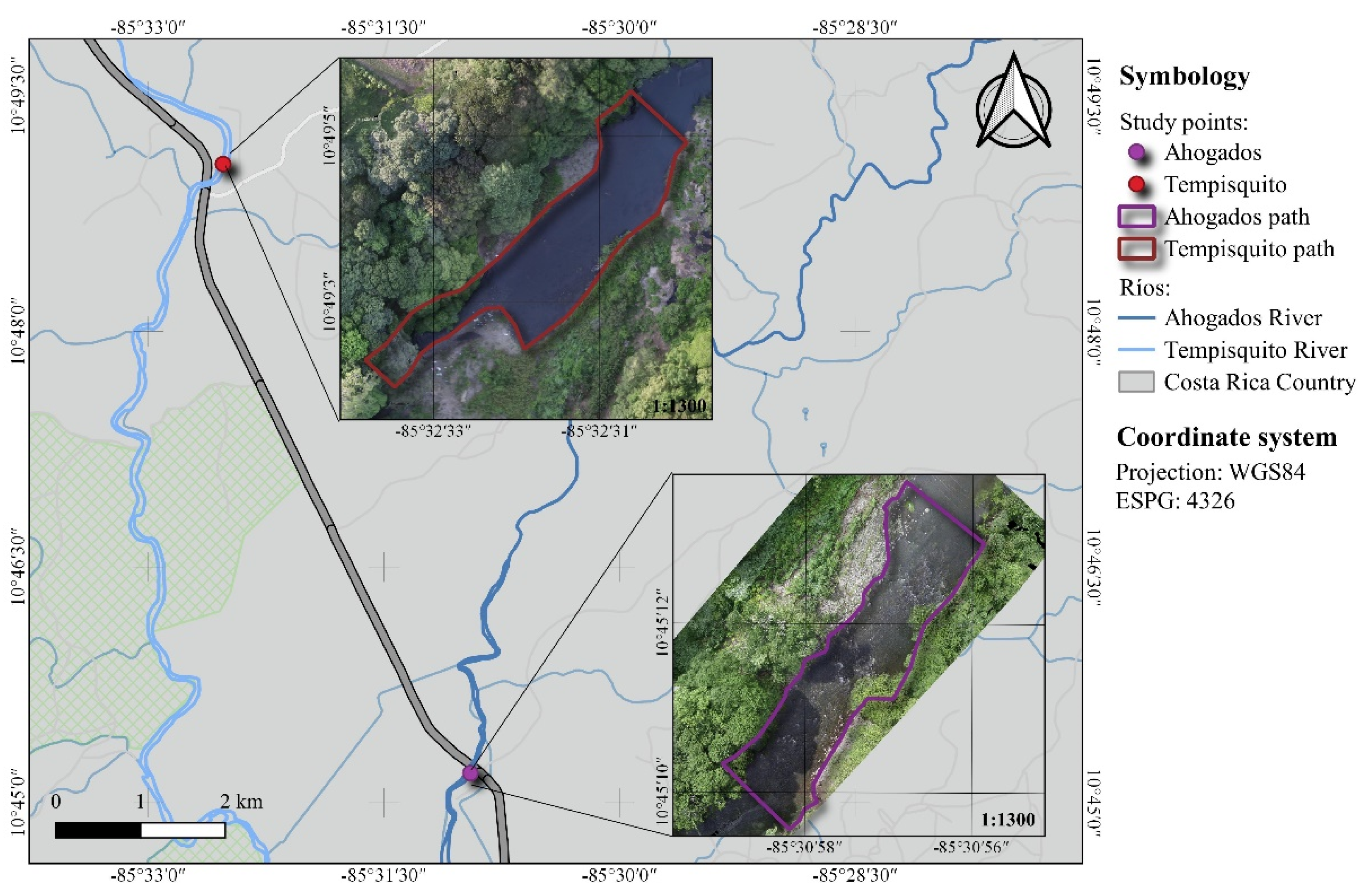
For this study, two paths were selected within the left margin of the Tempisque river basin in the upper zone of the basin located in the Ahogados and Tempisquito riverbeds (
Figure 1), these rivers originate in the foothills of the Guanacaste Mountain range. Due to its location on the Pacific coast of Costa Rica, climatic conditions in the basin are marked by a long dry season, causing many rivers to dry up completely, while in the rainy season they overflow; the average annual temperature is approximately 26.78 °C and the average elevation is 220 m.a.s.l. [
11].
Figure 2 shows the flow chart summarizing the methodology used in the study, which was based on the information gathered during the field visits and its subsequent processing, corresponding to the topographic and photogrammetric survey of the paths, and the sampling and granulometric analysis. The main percentiles for estimating particle roughness are the middle and upper percentiles of the particle size distribution, such as the 50th, 84th, and 90th percentiles [
12]. In this study, the particle size values corresponding to the 50th and 90th percentile were determined, additionally, an interpolation was carried out in the QGIS geographic information system, based on the points located in the study paths, obtaining the value by interpolation in areas within the path where sampling could not be carried out during the field visit.
The hydraulic modeling of the paths was carried out using the Iber 2.6 numerical modeling software. For the delimitation of the areas and their theoretical roughness values, four empirical equations known as “Strickler-type” were used (
Table 1), which it is possible to calculate the value of the Manning’s roughness coefficient as a function of the diameter of the particle. Considering that in Iber to perform an automatic roughness assignment on the mesh elements, a georeferenced file with the Manning’s roughness associated with the land use is required, the variety of roughness coefficient values had to be adapted to obtain a practical and feasible number of areas and land use (roughness) values, that is why the values were shortened to a limit of three decimal places.
Subsequently, the calibration of the eight bidimensional hydraulic models was accomplished using the “trial and error” process, starting from the results obtained in the simulation with the theoretical roughness.
The area of the water pattern formed by the channel of the study path (observed data) and the area of the water simulated by the program (simulated data) was compared quantitatively and spatially. Manually, the theoretical roughness values were multiplied by different numerical factors, obtaining new calculated roughness values, which were entered in the preprocessing (roughness areas remain constant), performing the hydraulic modeling repeatedly, until the areas resembled. The calibration of the models was performed until the “error”, that is, the percentage difference between the observed data and the simulated data, was less than 10% since during this process it was observed that, for higher values of roughness coefficient, no significant changes were generated in the performance of the simulated area (Asim).
Once the value of the factor for each model that allowed the best fit between the data was identified, the empirical formulas used were modified, adjusting them to the new roughness values, starting from the real value of the diameter in each of the roughness areas formed by each equation, and the calculated diameter of the uncorrected equation was determined. The applied formula of
Table 1 depends on where the above data is derived from, which follows a structure as seen in Equation (1).
where
is the Manning’s roughness coefficient;
is the theoretical constant that varies according to each researcher’s formula;
is the particle diameter for a percentile
x, the percentile to be used varies according to each researcher’s formula;
is the theoretical exponent that varies according to each researcher’s formula.
Then, the ratio (
) between the calculated diameter and the actual diameter in each roughness area was calculated as shown in Equation (2), and then the average value of the ratios was determined.
Finally, the new constant
that replaced the value of the theoretical counter of the researchers’ formulas was estimated, following the next equation.
3. Results
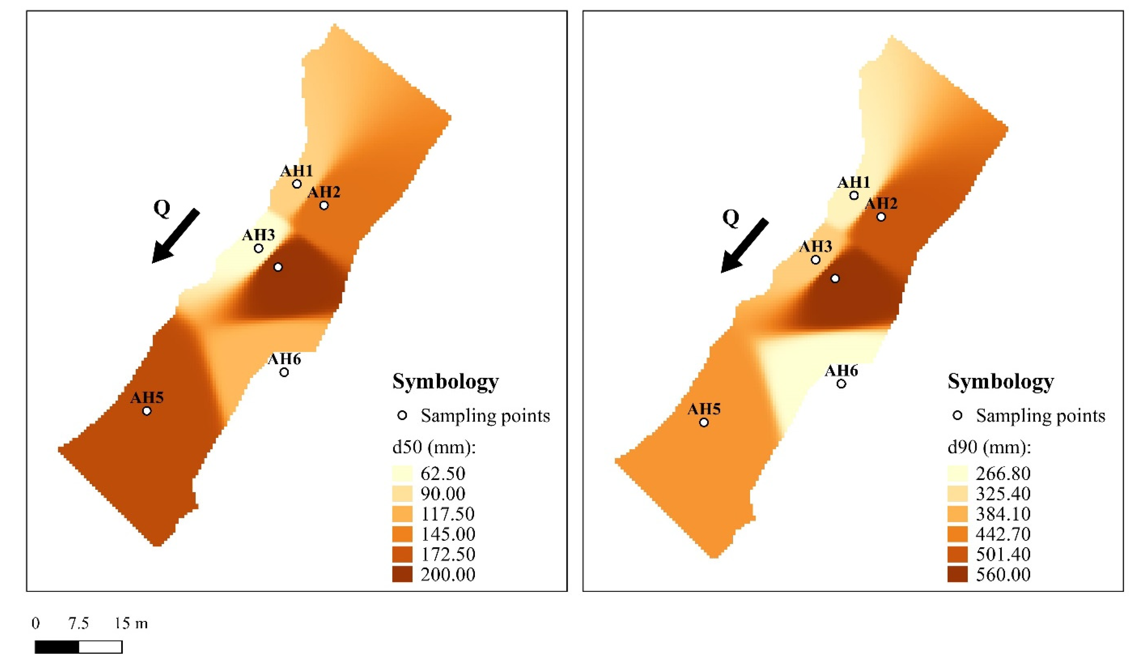
The pattern of the Ahogados riverbed has an area of 1849.90 m
2. From the
d50 range (
Figure 3) the particulate material within the bed is classified as cobble according to the Gallegos scale [
15], while in the Wentworth scale [
16] the majority of the bed is a cobble, except for the areas adjacent to sampling point AH3 which is classified as pebble gravel. It can be observed that in the six sampling points there are diameters greater than 256 mm, which is reflected in the d
90 values and evidence of the presence of boulder gravel along the bed.
The Ahogados River has an average particle diameter of 190.74 mm (d50 mean: 135.25 mm, and d90 mean: 398.97 mm).
On the other hand, the pattern of the Tempisquito riverbed study path is 1798.30 m
2. The bed particulate material is classified from
d50 as pebble gravel in the areas near points TQ1 to TQ7, TQ9 to TQ11, TQ13, TQ15 to TQ17, and TQ19 and as a boulder in the areas around points TQ8, TQ12, TQ14, and TQ18 according to the Wentworth scale [
16], while according to the Gallegos scale [
15] the entire bed of the channel is classified as cobble gravel (
Figure 4).
The Tempisquito River has an average particle diameter of 58.37 mm (d50 mean: 53.71 mm, and d90 mean: 119.43 mm).
Figure 5 and
Figure 6 show the areas and the different roughness values generated by the empirical equations for the Ahogados and Tempisquito rivers, respectively. The roughness values with factor 1.0 are theoretical, i.e., those obtained by applying the formulas in
Table 1. The values of the factors and roughness inside the red box were those where a difference between the areas (observed and simulated) of less than 10% was obtained and selected for subsequent modification of the equations.
The factors that showed an area difference of less than 10% in the Ahogados river path are 2.5 (9.26%), 2.7 (9.04%), 2.1 (9.09%), and 2.0 (9.35%) and in the Tempisquito river reach are 1.1 (3.98%), 1.2 (3.89%), 1.0 (3.78%) and 1.0 (3.66%), for the Strickler, MPM, Bray d50 and, Bray d90 equations, respectively.
Regarding the roughness values obtained for the factors mentioned above, in the Ahogados river course, these ranges are 0.075–0.090 (
Figure 5a), 0.081–0.092 (
Figure 5b), 0.076–0.092 (
Figure 5c) and, 0.080–0.090 (
Figure 5d), and in the Tempisquito river path, these ranges are 0.026–0.036 (
Figure 6a), 0.026–0.041 (
Figure 6b), 0.029–0.041 (
Figure 6c), and 0.030–0.044 (
Figure 6d), for the Strickler, MPM, Bray
d50 and Bray
d90 equations, respectively.
Table 2 shows the value of the new constant for the different researchers’ formulas, in a new equation.
4. Discussion
4.1. Grain Size Analysis
By comparing the results of the granulometric analysis in both paths, it can be generally determined that both channels are rivers with beds superficially formed by gravel and boulders; according to Church and Ferguson [
17], most of the rivers in highland areas have this type of bed, with
d50 in a range of approximately 10 to 100 mm.
In the Ahogados river, diameters greater than 256 mm were identified, which evidenced the presence of boulder gravel in the riverbed, while in the Tempisquito river, this type of diameter was scarce or even null in many of the sampling points. Regarding the identification of sands, in none of the sampling points of both paths were diameters of this type of material measured, firstly because the sampling techniques used are not adequate to counter this type of grains [
18], and secondly, because the sampling is superficial, even though, in rivers of this type (with cobble and pebble beds, and even boulder) the smaller particles are hidden by the larger particles, which form an “armoring” on the surface [
19,
20], however, it is pertinent to sample the surface materials since these are the ones that provide the roughness [
13,
21].
In addition to this analysis, in both study paths, lateral bars of gravelly material were observed on the banks of the riverbed (located in opposite areas), which are caused by the decrease in shear stress, lower flow velocity, causing the sediment load transported to be deposited on the banks of the channel [
19].
4.2. Correction of Empirical Equations
According to Jarret [
22], the values of the Manning’s roughness coefficient are usually much larger in rivers with higher gradients, and with a bed of cobble and boulders, making sense that the Ahogados river (
S = 1.42%) is the one that presented the higher roughness coefficients than the path of the Tempisquito river (
S = 0.74%).
It has been shown in several investigations that Strickler’s equation underestimates the roughness coefficient, the cause of this is that Strickler’s relationship was adjusted to relatively deep flows over nearly uniform beds, with a low slope and smaller form resistance [
23], so when conditions with low flows and high resistance are present, it is necessary to incorporate a relationship between the depth and grain size to estimate roughness [
9,
24] (these are the “power-based” and “semi-logarithmic-based” formulas). Other parameters that also influence Manning’s roughness coefficient apart from grain size are energy slope and hydraulic radius [
25].
The study by Ferguson [
23] indicates that the underestimation that comes from the Strickler equation is by a factor of 2 (on average, between half and double), being in this case, for the Ahogados river the calibration factor of 2.5, and in the Tempisquito river of 1.1.
Analyzing the study by Kim et al. [
13], who used the three classes of empirical equations to estimate the roughness coefficient for a gravel-bed river, they obtained with the Limerinos equation (a “semi-logarithmic-based” formula) the closest value to its roughness coefficient based on the field measurement; comparing this value only with the empirical “Strickler-type” equations, the Bray equations (
d50 and
d90) were the closest, while the Strickler and MPM equations underestimated it. In this case, in the Ahogados river path, it was the Bray equations that required a smaller factor to obtain an error of less than 10%; and in the Tempisquito river path, it was not necessary to apply any factor to obtain an even smaller error.
The models of the Tempisquito river path obtained the lowest percentages in the four empirical equations, in contrast to the models of the Ahogados river path. This behavior in the calibration of both paths derives from the need for the availability of field data to be able to feed and calibrate the numerical model [
6]. According to Horritt [
26], to calibrate a numerical model from the floodplain and roughness, the flow resistance coefficients must be spatially variable (heterogeneous) to improve the model performance, also, this same author refers that the success of the calibration is always a function of the uncertainty of the observed data.
The Tempisquito river path is the one that feeds the numerical model the most since the greatest amount of information was obtained from it during the field visits, specifically the granulometry information, which is the basis for the roughness coefficients in this study. While the Ahogados river path required a more extensive and partial calibration process because it lacked field data, which had to be assumed during processing (interpolation of granulometric data).
According to Pinos and Timbe [
27], the lack or non-existence of information hinders the calibration of the model. This was reflected in the results of the calibration process, obtaining a lower error for the Tempisquito river than for the Ahogados river.
To obtain high roughness values from the diameter of the bed material, a proportional constant was demanded, that is why the ratio calculated with Equation (2), the calculated diameter value is in the numerator and the real one in the denominator. According to Yen [
14] with the statistical analysis of different researchers’ tests it has been shown that varying the theoretical exponent (in Equation (1)) has very little influence on the results, however, Ferguson [
23] indicates that it should not always be assumed that this value is equal to 1/6 in all circumstances, on the other hand, concludes that the selection of a different grain diameter does not drastically affect the results.
5. Conclusions
Based on the grain size analysis of the riverbeds both study paths are rivers with coarse bed material, mainly composed of cobble and pebbles gravel. Considering the granulometry and topography, the channels under study are defined as mountain rivers.
The underestimation of the roughness coefficient generated by Strickler’s equation (1923) was confirmed by several researchers, and a correction was made by calibrating the hydraulic model.
The equations of Bray (1979) obtained the best results, delivering lower degree errors at a smaller factor value, being 2.1 and 2.0 in the Ahogados river, and 1.0 and 1.0 in the Tempisquito river, for Bray d50 and Bray d90, respectively.
The hydraulic models of the Tempisquito river study path presented the lowest errors, mainly because this path had more field data (granulometry) to feed the numerical model, and because the Ahogados river path, having a larger granulometry in the riverbed, requires higher roughness values to define the real hydraulic resistance of the flow.
With the new empirical equations adjusted in both study paths, it is possible to calculate the already calibrated roughness in rivers of the North Pacific of Costa Rica, as a function of the bed grain size.
From the results obtained in this study, it was shown that granulometric sampling has a considerable impact on model calibration, so it is suggested to increase the number of data collection points, as well as the number of samples (minimum 75) in studies of riverbeds, to obtain a greater heterogeneity that characterizes the morphology of the substrate.
In future research, it is recommended to work with other parameters on which the hydraulic resistance depends to estimate the roughness coefficient.


 ,
, 


