1. The Purpose of Bioprocess Simulation
One of the central goals of bioprocess design and analysis is to determine what resources are required to produce the desired annual amount of product. The resources in question include the process equipment, materials, utilities, and labor. Additional goals may include answering some of the following questions: Can the product be manufactured in an existing facility or is a new plant required? What is the total capital investment for a new facility? What is the manufacturing cost? How long does a single batch take? What is the minimum time between consecutive batches? Which process steps or resources are the likely production bottlenecks? What process and equipment changes can increase throughput? What is the environmental impact of the process? Which design is the “best” (fastest or least expensive) among several plausible alternatives?
The specific questions which must be evaluated, and the level of accuracy of the answers, depend upon the stage of development for a given product. The typical stages of development and commercialization, and the activities associated with those stages, are shown in
Figure 1 [
1,
2,
3]. At the preliminary stage of idea generation, process simulation is mainly used for assessing potential projects in order to determine which ones justify further effort and resources, and to “weed out” projects with less potential.
In process development, scientists and engineers investigate the various options available for synthesizing, purifying, characterizing, and formulating the final product. At this stage, simulation tools are used to evaluate alternative processing scenarios from an economic, cycle time reduction, and environmental point of view. In addition, cost-of-goods analysis facilitates identification of key steps of a process, which have high capital or operating costs or low yield and production throughput. The findings from the cost-of-goods analysis can then be used to determine what types of lab and pilot plant studies should be performed in order to improve those high-cost or low-yield sections of the process. The ability to perform “virtual experiments” and process analysis on a computer therefore reduces the amount of costly and time-consuming lab and pilot plant work by focusing the organization on potential process improvements that can have the greatest impact. Furthermore, cost analysis at the process development stage facilitates decisions related to in-house manufacturing versus outsourcing.
Figure 1.
Benefits from the use of computer aids.
Figure 1.
Benefits from the use of computer aids.
When a process progresses from development to manufacturing, simulation tools facilitate activities such as technology transfer, process fitting, and facility design. For example, the availability of a detailed process model enables efficient technology transfer by providing a comprehensive description of the process in a format that can be easily understood and modified by the recipients. Adjustments to the model are required when moving the process from the development site to a manufacturing site in order to scale up the process to the ideal size for the manufacturing-scale equipment, define cycling of certain steps (for equipment that is too small to handle a batch in one cycle), etc. In addition, if a new plant must be designed or an existing plant must be retrofitted for the process, the model can be used to determine the size of the equipment as well as the required capacity of supporting utility systems that will need to supply steam, electricity, purified water, etc. Estimations of the plant’s expected labor requirements are also done with such tools.
Once a process has been implemented within the manufacturing facility, simulation tools are used for debottlenecking studies and on-going optimization of that process. In addition, multiproduct plant modeling tools play a very important role in production planning and scheduling. They facilitate capacity analysis and long term planning, and also enable day-to-day production scheduling by accounting for constraints related to the limited availability of resources such as equipment, labor, utilities, material inventories,
etc. Furthermore, production scheduling tools fill the gap between the plant floor and the high-level tools used for Enterprise Resource Planning and Manufacturing Resource Planning [
4,
5]. Manufacturing Resource Planning (MRP) tracks the material requirements for a particular manufacturing operation. A second generation version of MRP (MRP II) adds production planning that accounts for plant capacity. Enterprise Resource Planning (ERP) increases the planning scope to include items such as finance and manpower planning. The objective of resource planning is to ensure that all the resources needed to fulfill production orders are in place. The production schedules generated by ERP and MRP II tools are generally based on rough process representations and approximate plant capacities that do not take all plant resource limitations into account. As a result, the solutions generated by ERP/MRP II tools may not actually be feasible, especially for complex multiproduct facilities operating at high capacity utilization. This often leads to delayed orders, which require expensive expediting and/or necessitate the maintenance of large inventories in order to provide customer responsiveness. Therefore “Lean manufacturing” concepts, such as just-in-time production (JIT), low work-in-progress (WIP), and low final product inventories cannot be implemented without using production scheduling tools that can accurately estimate capacity.
Sensitivity analyses are greatly facilitated by process simulation tools as well. The objective of these studies is to evaluate the impact of critical processing parameters on key performance indicators (KPIs) such as cycle times, plant throughput, and production cost.
2. Detailed Modeling of Single Batch Bioprocesses
Modeling and analysis of integrated batch bioprocesses is facilitated by process simulators. Simulation tools were first used in the chemical and petrochemical industries in the early 1960s. Simulators for these industries were designed primarily to model steady-state (continuous) processes as well as certain transient behaviors of these processes (e.g., startups, shutdowns, and perturbations). However, continuous modeling cannot account for the sequential nature of operations in batch and semi-continuous processes. These types of processes are modeled most effectively with batch process simulators that can account for time-dependency and sequencing of events. The first such process simulator was named BATCHES. This program was commercialized in the mid-1980s by Batch Process Technologies, a Purdue University spin-off headquartered in West Lafayette, IN. All of its operation models are dynamic, and simulation using BATCHES always involves integration of differential equations over a period of time. In the mid-1990s, Aspen Technology (Burlington, MA, USA) introduced Batch Plus (later renamed Aspen Batch Process Developer), a recipe-driven simulator that targeted batch pharmaceutical processes. Around the same time, Intelligen (Scotch Plains, NJ, USA) introduced SuperPro Designer. The initial focus of SuperPro Designer was on bioprocessing. Over the years, its scope has been expanded to support modeling of fine chemicals, pharmaceuticals, food processing, consumer products and other types of batch/semi-continuous processes. The SuperPro Designer structure for batch processes consists of a series of material and energy balance and design models for each processing task. The models, which may be either algebraic or dynamic, are solved in a sequential modular fashion. The remainder of this section will use an illustrative example to display the usage of process simulation for evaluating and optimizing integrated biochemical processes. The example represents a typical large-scale monoclonal antibody production process with a production rate of about 19.5 kg of monoclonal antibody (MAb) per batch. The process will be described in detail, including thorough material balance information. Then the execution of the process will be visualized through equipment occupancy charts, and the concept of cycle time analysis and reduction will be presented. Next, estimates of the capital and operating costs of the process will be provided, with detailed breakdowns for the costs of materials and consumables. Then the manufacturing cost impact of using multiple bioreactor trains, changing the bioreactor scale, and changing the product titer will be evaluated through sensitivity analysis. Analysis and assessment of additional bioprocesses can be found in the literature [
6].
2.1. Monoclonal Antibody Example Overview
Monoclonal antibodies (MAbs) are the fastest-growing segment within the biopharmaceutical industry [
7]. MAbs are currently used to treat various types of cancer, rheumatoid arthritis, psoriasis, severe asthma, macular degeneration, multiple sclerosis, and other diseases. More than 20 MAbs and Fc fusion proteins (therapeutic proteins linked to an immunoglobulin) are approved for sale in the United States and Europe and approximately 200 MAbs are in clinical trials for a wide variety of indications [
8,
9]. The market size for MAbs in 2010 was in excess of $35 billion [
10].
The high-dose demand for several MAbs translates into annual production requirements for purified product in the metric ton range. Such a process is modeled and analyzed with SuperPro Designer in the rest of this section.
Figure 2 displays the flowsheet of the overall process. The generation of the flowsheet was based on information available in the patent and technical literature combined with the authors’ engineering judgment and experience with such processes. The computer files for this example are available as part of the evaluation version of SuperPro Designer at the website:
www.intelligen.com/demo. Additional examples dealing with other biopharmaceuticals as well as commodity biological products are available at the same website.
To model an integrated process using SuperPro Designer, the first step is to develop a flowsheet that represents the overall process. The flowsheet is developed by selecting the required unit procedures and joining them with material flow streams. Next, it is necessary to initialize the flowsheet by specifying the materials used in the process and by specifying the operating conditions and performance parameters for the individual operations within each unit procedure. This sequence of steps will be explained in greater detail below.
Most biopharmaceutical processes operate in batch mode. This is in contrast to petrochemical and other high-throughput industries that use continuous processes. In continuous production, a piece of equipment performs the same action all the time. In batch processing, on the other hand, a piece of equipment goes through a cycle of operations. For instance, within
Figure 2 an inoculum preparation step (P-5 in SBR1) includes the following operations: SIP, SET UP, TRANSFER IN-1(media), TRANSFER IN-2 (inoculum), FERMENT (fermentation operation), TRANSFER OUT (emptying vessel), CIP (cleaning of equipment). In SuperPro, the set of operations that comprises a processing step is called a “unit procedure” (as opposed to a unit operation). The individual tasks contained in a procedure (e.g., Transfer in, Ferment, CIP,
etc.) are called operations. A unit procedure is represented on the screen with a single equipment icon. In essence, a unit procedure is the recipe that describes the sequence of actions required to complete a single processing step. The hierarchical representation of batch processes (also known as recipes) using unit procedures and operations is an approach that is recommended by the International Society of Automation (ISA) because it facilitates modeling, control, and scheduling of batch operations [
11].
Figure 2.
Monoclonal antibody production (MAb) flowsheet.
Figure 2.
Monoclonal antibody production (MAb) flowsheet.
For every relevant operation within a unit procedure, the simulator includes a mathematical model which performs material and energy balance calculations. Then, based on the material balance results, the simulator determines the necessary size of each equipment unit. If multiple operations within a given equipment unit have different capacity requirements, the simulator sets the unit’s size to be equal to the minimum size which still meets or exceeds every individual operation’s capacity requirement. This ensures the equipment will be large enough to meet the processing demands while simultaneously minimizing capital costs. Alternatively, if the equipment size is specified by the user, the simulator simply checks to make sure that the vessel is not overfilled. In addition, the tool checks to ensure that the vessel contents will not fall below a user-specified minimum volume (e.g., a minimum stir volume) for applicable operations.
2.2. Process Description
Upstream: The upstream part of this example process is split into two sections: the Inoculum Preparation section and the Cell Culture section. The inoculum is initially prepared in an 18-unit rack of 225 mL T-flasks. Next the material is moved to an eight-unit rack of 2.2 L roller bottles, then to a set of 100 L disposable bag bioreactors and subsequently to a set of 200 L disposable rocking bag bioreactors. An appropriate amount of sterilized media is fed to each unit in all four of these steps (3.6, 11.4, 43.6, and 175.4 L/batch, respectively). The broth is then moved to the first and subsequently to the second seed bioreactor (1200 L and 5000 L respectively). The media powder for the seed bioreactors is dissolved in water-for-injection (WFI) in two preparation tanks (MP-101 & MP-102). Then it is sterilized and fed to the reactors through 0.2 μm dead-end filters (DE-101 & DE-102).
In the Cell Culture section, serum-free low-protein media powder is dissolved in WFI in a stainless steel tank (MP-103). The solution is sterilized using a 0.2 μm dead-end polishing filter (DE-103). A stirred-tank bioreactor (BR-101) is used to grow the cells, which produce the therapeutic monoclonal antibody (MAb). The production bioreactor operates under a fed batch mode, drawing in additional concentrated media from another media preparation tank (MP-104) during the fermentation. Fed batch mode is used because high media concentrations are inhibitory to the cells. Therefore half of the media is added at the start of the process and the rest is fed at a variable rate during fermentation. The concentration of media powder in the initial feed solution is 17 g/L. The fermentation time is 12 days. The volume of broth produced per bioreactor batch is roughly 15,000 L, which contains approximately 30 kg of product (i.e., the product titer is approximately 2 g/L).
Downstream: Between major downstream unit procedures there are 0.2 μm dead-end filters, e.g., DE-108, to ensure sterility. The generated biomass and other suspended compounds are removed using a Disc-Stack centrifuge (DS-101). During this step, roughly 4% of the MAb product is lost in the solids waste stream, resulting in a product yield of 96%. The bulk of the contaminant proteins are removed using a Protein-A affinity chromatography column (C-101). The following operating assumptions were made for the column: (1) resin binding capacity is 15 g of product per L of resin; (2) the eluant or elution buffer is a 0.6% w/w solution of acetic acid and its volume is equal to five column volumes (CVs); (3) the product is recovered in 2 CVs of eluant with a recovery yield of 90%; and (4) the total volume of the solution for column equilibration, wash and regeneration is 14 CVs. The entire procedure takes approximately 26 h and requires a resin volume of 484 L. The protein solution is then concentrated five-fold and diafiltered 2× (in P-21/DF-101) using WFI as diluant. This step takes approximately 5 h and requires a membrane of 20 m2. The product yield is 97%. The concentrated protein solution is then chemically treated for 1.5 h with Polysorbate 80 to inactivate viruses (in P-22/V-111). An Ion Exchange chromatography step follows (P-24/C-102). The following operating assumptions were made for this step: (1) the resin’s binding capacity is 40 g of product per L of resin; (2) a gradient elution step is used with a sodium chloride concentration ranging from 0.0 to 0.1 M and a volume of 5 CVs; (3) the product is recovered in 2 CVs of eluant buffer with a yield on MAb of 90%; and (4) the total volume of the solutions for column equilibration, wash, regeneration, and rinse is 16 CVs. The step takes approximately 22 h and requires a resin volume of 211 L. Ammonium sulfate is then added to the IEX eluate (in P-25/V-109) to a concentration of 0.75 M to increase the ionic strength in preparation for the Hydrophobic Interaction Chromatography (P-26/C-103) that follows. The following operating assumptions were made for the hydrophobic interaction chromatography (HIC) step: (1) the resin binding capacity is 40 g of product per L of resin; (2) the eluant is a Sodium Chloride (4% w/w) Sodium Di-hydro Phosphate (0.3% w/w) solution and its volume is equal to 5 CVs; (3) the product is recovered in 2 CVs of eluant buffer with a recovery yield of 90%; and (4) the total volume of the solution for column equilibration, wash and regeneration is 12 CVs. The step takes approximately 22 h and requires a resin volume of 190 L. A viral exclusion step (DE-105) follows. It is a dead-end type of filter with a pore size of 0.02 μm. This step takes approximately 2.8 h. Finally the HIC elution buffer is exchanged for the phosphate buffered saline (PBS) solution and concentrated 1.5-fold (in DF-102). This step takes approximately 8 h and requires a membrane of roughly 10 m2. The 774 L of final protein solution is stored in twenty 50 L disposable storage bags (DCS-101). Approximately 19.5 kg of MAb are produced per batch. The overall yield of the downstream operations is 64.4%.
After the process specifications have been completed and the process model has been simulated, the full results may be viewed and analyzed. Results include material input and output compositions and amounts, equipment size calculations, process scheduling information, process costing, etc. Partial results for this example process are described in the following sections.
2.3. Material Balances
Table 1 provides a summary of the materials used by the process, with raw material requirements listed per year, per batch, and per kg of Main Product (MP). These results were calculated by the process simulator, based upon the input parameters specified for relevant operations such as material charges. Note the large amount of WFI utilized per batch. The majority of WFI is consumed for cleaning and buffer preparation.
In addition to calculating the overall raw material requirements, process simulators calculate the amounts and compositions of each individual stream (inputs, intermediates and outputs). This provides useful information for verifying results related to material transformations and separations, liquid and solid waste generation, emissions, equipment capacity requirements, etc.
Table 1.
Raw Material Requirements (MP = purified MAb).
Table 1.
Raw Material Requirements (MP = purified MAb).
| Material | kg/yr | kg/batch | kg/kg MP |
|---|
| Inoc Media Sltn | 4888 | 232.76 | 11.93 |
| WFI | 1,072,146 | 51,054.58 | 2617.62 |
| SerumFree Media | 9419 | 448.52 | 23.00 |
| H3PO4 (5% w/w) | 242,994 | 11,571.15 | 593.27 |
| NaOH (0.5 M) | 226,036 | 10,763.64 | 551.86 |
| Air | 867,389 | 41,304.23 | 2117.71 |
| Protein A Equil | 446,384 | 21,256.40 | 1089.84 |
| Protein A eluti | 202,216 | 9629.33 | 493.71 |
| Prot-A Reg Buff | 121,398 | 5780.86 | 296.39 |
| NaOH (0.1M) | 135,799 | 6466.60 | 331.55 |
| IEX-Eq-Buff | 66,503 | 3166.82 | 162.37 |
| IEX-Wash-Buff | 66,797 | 3180.80 | 163.08 |
| IEX-El-Buff | 3765 | 179.29 | 9.19 |
| NaCI (1 M) | 40,835 | 1944.51 | 99.70 |
| Amm. Sulfate | 2845 | 135.46 | 6.95 |
| HIC-Eq-Buff | 26,371 | 1255.75 | 64.38 |
| HIC-Wash-Buff | 62,681 | 2984.82 | 153.04 |
| HIC-El-Buff | 60,792 | 2894.86 | 148.42 |
| NaOH (1 M) | 65,709 | 3129.00 | 160.43 |
| PBS | 32,483 | 1546.83 | 79.31 |
| Polysorbate 80 | 2 | 0.08 | 0.00 |
| TOTAL | 3,757,452 | 178,926.28 | 9173.74 |
2.4. Scheduling and Cycle Time Reduction
As noted previously, a unique feature of batch process simulators (as opposed to continuous simulators) is their ability to model the time-dependent aspects of batch processes. This enables the automatic generation of a process schedule.
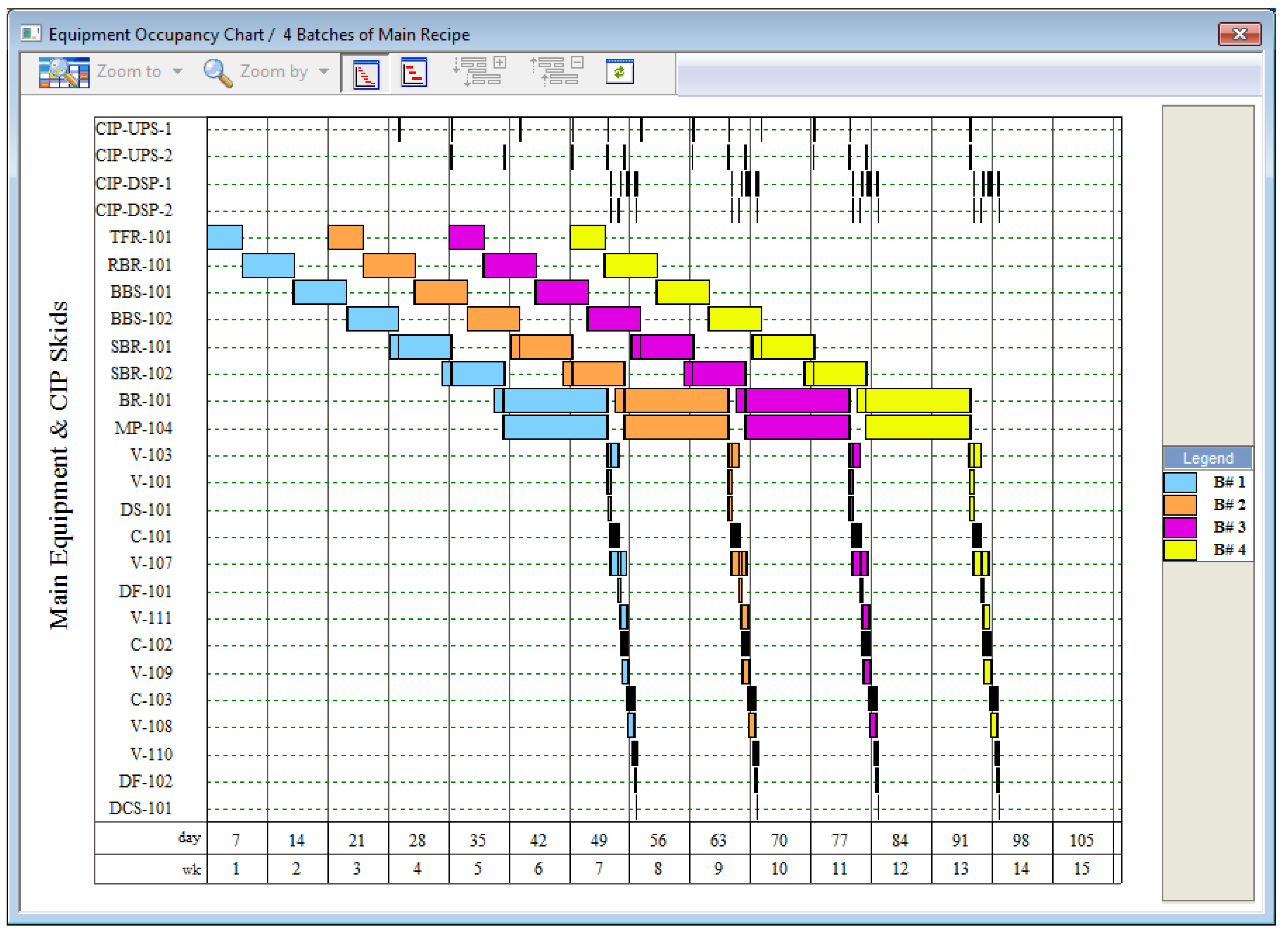
Figure 3 displays the schedule for four consecutive batches of this example process. The equipment units are shown on the vertical axis while the time is shown on the horizontal axis. The four batches are represented with four different colors. This figure shows the equipment occupancy for a plant that has a single production train. The cleaning-in-place (CIP) skids can be seen at the top of the figure. The other main equipment can be seen further down. Note that
Figure 3 does not show all equipment required for this process; various filters, mixing tanks, and other minor equipment have been excluded from the chart.
The batch time for this process is approximately 50 days. This is the time required from the start of inoculum preparation to the final product purification of a single batch. The cycle time—the time between consecutive batch starts—is determined by the cycle time bottleneck, which is the production bioreactor (BR-101) in this case. The minimum cycle time is just under 14 days and, for this example, has been rounded to exactly 14 days.
Based on the batch time, the batch cycle time, and an assumed plant uptime of 330 days/year, this plant can complete roughly 21 batches per year, producing approximately 410 kg/year of purified MAb. It is clear from
Figure 3 that under these conditions the downstream purification train is under-utilized since the purification train units are idle far more often than they are active. The cycle time of the process can be reduced (and the plant throughput increased) by installing multiple bioreactor trains that operate in staggered mode (out of phase) and feed the same purification train. For example,
Figure 4 represents a case where four bioreactors (BR-101, 101b, 101c, and 101d) feed a single purification train. Like
Figure 3,
Figure 4 does not show all the equipment used for this process—most of the inoculum preparation equipment and other minor equipment items have been excluded from the chart, and some of the downstream purification equipment is not shown. Unlike
Figure 3,
Figure 4 displays additional seed bioreactors as well as other upstream equipment that have been added in order to support the new bioreactors. With this four-bioreactor scenario the new cycle time is 3.5 days, which is one fourth of the original cycle time. Under these conditions, the plant processes 81 batches per year and produces approximately 1580 kg of MAb per year. Some biopharmaceutical companies have installed more than four bioreactor trains per purification train in order to achieve cycle times as low as two days. This maximizes plant throughput while minimizing capital cost per kg of product.
Although availability of a key equipment item (such as the production bioreactor in this example) is frequently the process bottleneck, in many cases other resources such as labor, utilities, and raw materials can become bottlenecks as well. Although resource requirements can be investigated for individual processes using process simulation tools, it generally makes more sense to evaluate these potential constraints in the context of an overall plant environment (with multiple processes running simultaneously). Evaluation and sizing of these types of shared resources will be covered in the Multiproduct Modeling section of this report (
Section 3).
Figure 3.
One bioreactor train feeding one purification train.
Figure 3.
One bioreactor train feeding one purification train.
Figure 4.
Four bioreactor trains feeding one purification train.
Figure 4.
Four bioreactor trains feeding one purification train.
2.5. Economic Evaluation
Accurate project cost analysis and economic evaluation are critical during late-stage development and commercialization of a product. For new products, if a company lacks a suitable manufacturing facility with sufficient available capacity, it must decide whether to build a new plant, retrofit an existing plant, or outsource the production. Building a new plant is a major capital expenditure and a very lengthy process. In order to make a well-informed decision on whether to build (or retrofit) a plant, management must have information on the capital investment required and the timeline to complete the facility. If a company chooses to outsource production instead, a cost-of-goods analysis provided by a process model can serve as the basis for discussion of the process and negotiation with contract manufacturers. Contract manufacturers usually base their offerings on requirements of facility/equipment utilization and labor per batch, which may be provided by the model.
The data from the preceding analysis can be leveraged to perform a financial evaluation of the process. To accomplish this, the cost of equipment is first estimated by the software using built-in cost correlations that are based on data derived from a number of vendors and literature sources. The fixed capital investment is then estimated based on equipment costs and various multipliers. Some of these multipliers are equipment-specific (e.g., installation cost) while others are process-specific (e.g., cost of piping, buildings,
etc.). This approach is described in detail in the literature [
12,
13,
14]. The rest of this section provides a summary of SuperPro Designer’s cost analysis results for this example process.
Table 2.
Major Equipment Specification and Purchase Costs (Year 2013 prices in US $).
Table 2.
Major Equipment Specification and Purchase Costs (Year 2013 prices in US $).
| Quantity | Name | Description | Unit Cost ($) | Total Cost ($) |
|---|
| 4 | BBS-101 | Rocking Bioreactor Skid | 548,000 | 2,192,000 |
| | | Container Volume = 100 L | | |
| 6 | BBS-102 | Rocking Bioreactor Skid | 548,000 | 3,288,000 |
| | | Container Volume = 200 L | | |
| 1 | MP-101 | Blending Tank | 186,000 | 186,000 |
| | | Vessel Volume = 800 L | | |
| 3 | SBR-101 | Seed Bioreactor | 1,201,000 | 3,603,000 |
| | | Vessel Volume = 1200 L | | |
| 1 | MP-102 | Blending Tank | 226,000 | 226,000 |
| | | Vessel Volume = 3200 L | | |
| 3 | SBR-102 | Seed Bioreactor | 1,351,000 | 4,053,000 |
| | | Vessel Volume = 4800 L | | |
| 1 | MP-103 | Blending Tank | 257,000 | 257,000 |
| | | Vessel Volume = 11,000 L | | |
| 4 | MP-104 | Blending Tank | 197,000 | 788,000 |
| | | Vessel Volume = 1200 L | | |
| 4 | BR-101 | Bioreactor | 1,948,000 | 7,792,000 |
| | | Vessel Volume = 19,000 L | | |
| 1 | V-101 | Blending Tank | 280,000 | 280,000 |
| | | Vessel Volume = 17,000 L | | |
| 1 | DS-101 | Disk-Stack Centrifuge | 469,000 | 469,000 |
| | | Throughput = 2000 L/h | | |
| 1 | V-103 | Blending Tank | 276,000 | 276,000 |
| | | Vessel Volume = 16,000 L | | |
| 1 | C-101 | PBA Chromatography Column | 622,000 | 622,000 |
| | | Column Volume = 480 L | | |
| 1 | V-107 | Blending Tank | 236,000 | 236,000 |
| | | Vessel Volume = 4300 L | | |
| 1 | DF-101 | Diafilter | 65,000 | 65,000 |
| | | Membrane Area = 20 m2 | | |
| 1 | V-111 | Blending Tank | 188,000 | 188,000 |
| | | Vessel Volume = 870 L | | |
| 1 | C-102 | PBA Chromatography Column | 451,000 | 451,000 |
| | | Column Volume = 210 L | | |
| 1 | V-109 | Blending Tank | 204,000 | 204,000 |
| | | Vessel Volume = 1500 L | | |
| 1 | C-103 | PBA Chromatography Column | 439,000 | 439,000 |
| | | Column Volume = 190 L | | |
| 1 | V-108 | Blending Tank | 199,000 | 199,000 |
| | | Vessel Volume = 1300 L | | |
| 1 | V-110 | Blending Tank | 199,000 | 199,000 |
| | | Vessel Volume = 1300 L | | |
| 1 | DF-102 | Diafilter | 42,000 | 42,000 |
| | | Membrane Area = 10 m2 | | |
| | | Unlisted Equipment | | 9,661,000 |
| | | | GRAND TOTAL | 35,716,000 |
Table 3.
Fixed Capital Estimate Summary (Year 2013 prices in US $).
Table 3.
Fixed Capital Estimate Summary (Year 2013 prices in US $).
| Total Plant Direct Cost (TPDC) (physical cost) |
|---|
| Equipment Purchase Cost | 35,716,000 |
| Installation | 18,960,000 |
| Process Piping | 12,501,000 |
| Instrumentation | 14,286,000 |
| Insulation | 1,071,000 |
| Electrical | 3,572,000 |
| Buildings | 107,147,000 |
| Yard Improvement | 5,357,000 |
| Auxiliary Facilities | 14,286,000 |
| TPDC | 212,896,000 |
| Total Plant Indirect Cost (TPIC) |
| Engineering | 53,224,000 |
| Construction | 74,514,000 |
| TPIC | 127,738,000 |
| Total Plant Cost (TPC = TPDC+TPIC) |
| TPC | 340,634,000 |
| Contractor’s Fee & Contingency (CFC) |
| Contractor’s Fee | 17,032,000 |
| Contingency | 34,063,000 |
| CFC | 51,095,000 |
| Direct Fixed Capital Cost (DFC = TPC+CFC) |
| DFC | 391,729,000 |
Table 4.
Operating Cost Summary (Year 2013 prices in US $).
Table 4.
Operating Cost Summary (Year 2013 prices in US $).
| Cost Item | $ | % |
|---|
| Raw Materials | 13,229,000 | 9.89 |
| Labor-Dependent | 18,536,000 | 13.85 |
| Facility-Dependent | 71,215,000 | 53.22 |
| Laboratory/QC/QA | 9,268,000 | 6.93 |
| Consumables | 21,460,000 | 16.04 |
| Waste Treatment/Disposal | 75,000 | 0.06 |
| Utilities | 36,000 | 0.03 |
| TOTAL | 133,817,000 | 100.00 |
Table 5.
Consumables Cost Breakdown (Year 2013 prices in US $).
Table 5.
Consumables Cost Breakdown (Year 2013 prices in US $).
| Consumable | Unit Cost($) | AnnualAmount | | Annual Cost($) | % |
|---|
| 2.2 L Roller Bottle | 6 | 648 | item | 3888 | 0.02 |
| Dft DEF Cartridge | 1000 | 1134 | item | 1,134,000 | 5.28 |
| 225 mL T-Flask | 2 | 1458 | item | 2916 | 0.01 |
| Dft Membrane | 400 | 121 | m2 | 48,469 | 0.23 |
| 50 L Bag | 5 | 1620 | item | 8100 | 0.04 |
| Viral Exclusion Membrane | 13,356 | 81 | item | 1,081,836 | 5.04 |
| Protein A | 6000 | 2613 | L | 15,678,296 | 73.06 |
| SP-Sepharose High Performance | 1200 | 1027 | L | 1,231,844 | 5.74 |
| HIC Butyl Sepharose High Perf. | 2050 | 924 | L | 1,893,960 | 8.83 |
| Sartorius CultiBag RM 100 | 840 | 162 | item | 136,080 | 0.63 |
| Sartorius CultiBag RM 200 | 990 | 243 | item | 240,570 | 1.12 |
| TOTAL | | | | 21,459,958 | 100.00 |
Table 6.
Raw Materials Cost Breakdown (Year 2013 prices in US $).
Table 6.
Raw Materials Cost Breakdown (Year 2013 prices in US $).
| Bulk Material | Unit Cost ($) | Annual Amount (kg) | Annual Cost ($) | % |
|---|
| Inoculation Media | 6.15 | 18,854 | 115,893 | 0.88 |
| WFI | 0.15 | 4,135,421 | 620,313 | 4.69 |
| SerumFree Media | 300.00 | 36,330 | 10,899,050 | 82.39 |
| H3PO4 (5% w/w) | 0.14 | 937,263 | 133,560 | 1.01 |
| NaOH (0.5 M) | 0.25 | 871,855 | 213,657 | 1.62 |
| Protein A Equil | 0.15 | 1,721,769 | 263,344 | 1.99 |
| Protein A eluti | 0.15 | 779,976 | 119,711 | 0.90 |
| Prot-A Reg Buff | 0.17 | 468,249 | 78,539 | 0.59 |
| NaOH (0.1M) | 0.24 | 523,795 | 127,345 | 0.96 |
| IEX-Eq-Buff | 0.19 | 256,512 | 47,746 | 0.36 |
| IEX-Wash-Buff | 0.22 | 257,645 | 56,884 | 0.43 |
| IEX-El-Buff | 0.35 | 14,522 | 5045 | 0.04 |
| NaCI (1 M) | 0.37 | 157,505 | 58,008 | 0.44 |
| Amm. Sulfate | 8.00 | 10,972 | 87,775 | 0.66 |
| HIC-Eq-Buff | 0.91 | 101,716 | 92,438 | 0.70 |
| HIC-Wash-Buff | 0.54 | 241,771 | 130,073 | 0.98 |
| HIC-El-Buff | 0.31 | 234,484 | 71,432 | 0.54 |
| NaOH (1 M) | 0.34 | 253,449 | 85,220 | 0.64 |
| PBS | 0.18 | 125,293 | 22,839 | 0.17 |
| Polysorbate 80 | 1.83 | 6 | 12 | 0.00 |
| TOTAL | | | 13,228,884 | 100.00 |
Table 2 provides a list of the major equipment items in this project, along with their purchase costs. The total equipment cost for a plant of this capacity (four production bioreactors each having a working volume of 15,000 L and a total volume of around 19,000 L) is approximately $36 million. Almost one quarter of the equipment cost is associated with the four production bioreactors. The cost of filters and inoculum preparation items that are seen in
Figure 2 but are missing from the table are accounted for under the “Unlisted Equipment” item near the bottom of this table. This economic evaluation also takes into account the vessels required for buffer preparation and holding that are not included in
Figure 2. A full model that includes all buffer preparation and holding activities and other advanced process modeling features can be downloaded from
www.intelligen.com/demo.
Table 3 displays the various items included in the direct fixed capital (DFC) investment. The total DFC for a plant of this capacity is around $392 million, or approximately 11 times the total equipment cost. The total capital investment, which includes the cost of start-up and validation, is around $512 million.
Table 4 provides a summary of the operating cost for this project. The total annual operating cost is $134 million, resulting in a unit production cost of around $84.7/g (1,580 kg of purified product are produced annually). The facility-dependent cost is the most important item, accounting for roughly half of the overall operating cost. This is common for high value biopharmaceuticals. Depreciation of the fixed capital investment and maintenance of the facility are the main contributors to this cost. Consumables and Labor are the second and third largest operating costs, at 16% and 14% of the total, respectively. Consumables include the cost of chromatography resins and membrane filters that need to be replaced on a regular basis. The replacement of the Protein-A resin accounts for 73% of the total consumables cost (see
Table 5). A unit cost of $6000/L and a replacement frequency of 60 cycles were assumed for the Protein-A resin. Raw materials account for around 10% of the overall cost. The main raw material cost contributor is Serum Free Media, which accounts for 82% of the raw materials cost (see
Table 6). This is based on an assumed price of $300/kg for Serum Free Media in dry powder form. Approximately 72% of the manufacturing cost is associated with the upstream section (inoculum preparation and fermentation) and 28% with the downstream section (product recovery and purification).
2.6. Sensitivity Analysis
After a model of the proposed process has been developed on the computer, tools like SuperPro Designer can be used to ask and readily answer “what if” questions and to carry out sensitivity analysis with respect to key design variables. For example, there may be uncertainty regarding the annual demand for the final product, the product yield during fermentation at full-scale production, the recovery in the downstream purification units, etc. These factors may have a large impact on the overall economics of a process. Therefore it is important to understand the effect of changing these types of variables in order to determine whether or not it is wise to move forward with a project. In this example, sensitivity analyses were performed to understand the impact on unit production cost of the number of bioreactor trains, the product titer, and the bioreactor volume.
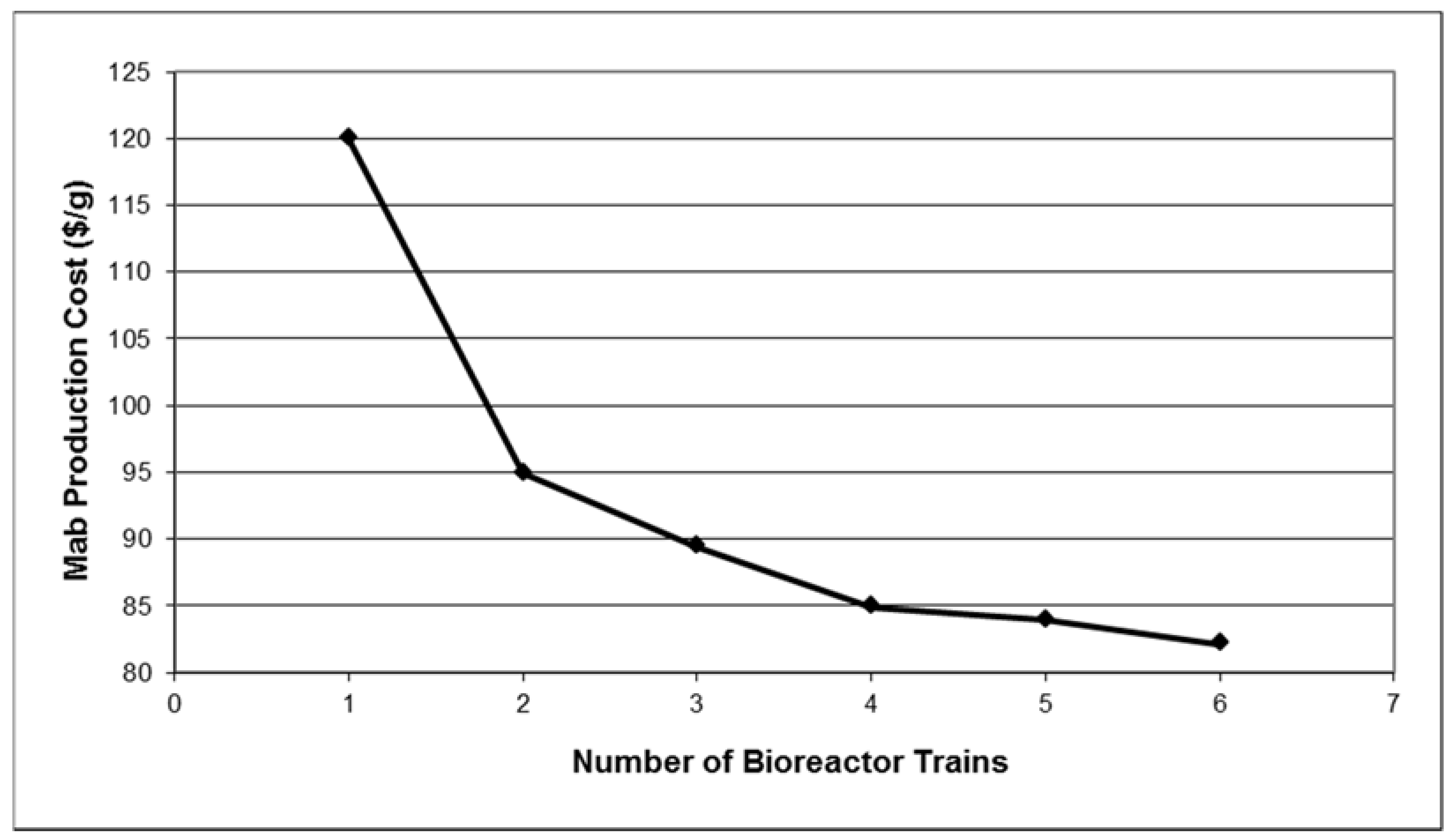
Figure 5 displays the impact of bioreactor trains on the unit production cost. Note that the cost analysis calculations in
Section 2.5 correspond to the case of four production bioreactors (each having a working volume of 15,000 L) feeding a single purification train and resulting in a unit cost of around $85/g. In contrast, if just a single bioreactor train feeds the purification train, the manufacturing cost increases by over 80%. Furthermore, as production bioreactors are added to the plant (while keeping a single purification train), the unit cost drops slowly and asymptotically approaches a value of around $80/g. Multiple production bioreactors that feed a single purification train lead to reduced manufacturing cost because the plant throughput is increased (since it is proportional to the number of bioreactors) without the need for additional capital investments in the purification train. A ratio of four or five bioreactor trains per purification train is probably the optimum number for cell culture processes that have a fermentation time of around twelve days. Such processes typically operate with cycle times ranging between 3.5 and 2.5 days.
Figure 6 displays the impact of product titer and bioreactor volume on the unit production cost. All points correspond to four production bioreactors feeding a single purification train. For low product titers, the bioreactor volume has a considerable effect on the unit production cost. For instance, for a bioreactor product titer of 1 g/L, going from 10,000 L to 20,000 L of production bioreactor volume reduces the unit cost by about $64/g (from approximately $194/g to $130/g). On the other hand, for high product titers (e.g., around 2.5 g/L), the impact of bioreactor scale is not as important (the differential is only about $27/g). This is because at high product titers, a higher percentage of the manufacturing cost is associated with the purification train. Therefore the bioreactor volumes (and their associated costs) are less relevant. It is therefore wise to shift R&D efforts from cell culture to product purification as the product titer in the bioreactor increases. A key assumption for the results of the sensitivity analysis is that the composition and cost of the cell culture media is independent of product titer.
Figure 5.
Production cost of MAb as a function of the number of bioreactor trains.
Figure 5.
Production cost of MAb as a function of the number of bioreactor trains.
Figure 6.
Production cost of MAb as a function of product titer and production bioreactor volume.
Figure 6.
Production cost of MAb as a function of product titer and production bioreactor volume.
3. Design and Operation of Multi-Product Facilities
The focus of batch process simulation, as described earlier in this report, is on the detailed modeling of a single batch process. The outputs of such models include thorough material and energy balances, resource capacity and time utilization, equipment sizing information, capital and operating cost results, etc. Such models facilitate scale up/down calculations, cycle time analysis, economic evaluation, technology transfer, and process fitting. The primary objective of such models is to optimize processes under development.
In contrast, modeling of multiproduct batch plants is focused on evaluating the interactions among multiple processes running concurrently and/or sequentially in a plant. This is important since most biotech facilities are multiproduct plants. Furthermore, in most applications of multiproduct plant modeling, the process flows and equipment sizes are quite well defined. As a result, such models place less emphasis on process design calculations and more emphasis on timing and utilization of shared resources such as equipment, utilities, labor, and inventories of materials. The sharing of resources across multiple processes renders the design and operation of multiproduct facilities more challenging than design and operation of a single isolated process, and computer models developed for such environments must capture the interaction among production lines at the facility level. In other words, during the design of multiproduct facilities, computer models must be able to determine the overall resource requirements for many different processes which will be run simultaneously. After the facility is built, models may be used to determine the manufacturing capacity for different production scenarios. They are also used to generate feasible production schedules that respect all major production constraints. Production scheduling results are typically communicated through Gantt charts and reports that provide information on tasks that need to be executed during a certain time period. Furthermore, due to the inherent variability of biological processes, scheduling tools employed in the biopharmaceutical industry must be able to efficiently handle conflict resolution and rescheduling.
3.1. Applications of Multiproduct Plant Modeling
Typical applications of multiproduct plant modeling include:
Each of these applications is explained in greater detail below:
Capacity Analysis and Strategic Planning—Capacity analysis models provide a high-level estimate of the manufacturing capabilities of existing or planned plants, based on the availability of key resources such as production lines. The main objectives may include determining the production rate for existing facilities or determining which of several facilities is best for a new product. These types of models may also be used to estimate the demand for raw materials that need to be purchased, especially those requiring long lead times. Capacity analysis models tend to rely on simplified recipes since they need to cover the production of many different products over a period of a year or longer.
Production Scheduling—The objective of this activity is to assign specific resources to each production campaign, estimate the start times for campaigns and batches, and determine the time horizon for producing specific quantities of a particular combination of products in order to meet market demands. The time horizon is usually weeks to months but it may extend to a year for certain industries such as biopharmaceuticals.
Facility Design and Debottlenecking—This is the inverse of the capacity analysis problem. During the design of new facilities or the retrofit of existing ones, multiproduct plant models are used to estimate resource levels required to achieve a certain production volume within a given time period. Such models should account for the occupancy of all equipment and resources whose supply may be limited. Apart from raw materials, typical resources include main equipment (e.g., reactors, filters, dryers,
etc.), auxiliary equipment (e.g., shared pipe segments, transfer panels, cleaning equipment), utilities (e.g., steam, purified water, and electrical power), and various types of labor. Engineering companies involved in the design of new facilities frequently use these types of models [
3]. Debottlenecking activities are aimed at increasing the production of existing manufacturing lines and facilities, and they may result in improvements to production scheduling and/or retrofitting of facilities in order to increase production capacity.
The above applications require plant models with increasing levels of detail. Capacity analysis models require the least detail because they do not need to capture specific details about how to execute the processes. Production can be represented with simplified campaigns associated with key equipment items (or manufacturing lines) that are likely to limit throughput. Long term raw material planning utilizes models with a level of detail similar to those of capacity analysis. In contrast, production scheduling models need to communicate when to execute process operations. Therefore they require greater detail than capacity analysis models in order to account for the utilization of all main equipment items as well as critical auxiliary equipment and other key resources (i.e., ones with high utilization that are likely bottlenecks). Finally, the most detailed models are required for cycle time reduction and debottlenecking studies, which must account for the occupancy of all equipment (main and auxiliary) as well as all other resources (e.g., utilities and materials) whose supply may be limited at any point in time. Although highly-detailed models such as the ones used for design and debottlenecking studies could theoretically be used for short term production scheduling, it is advisable to keep models as simple as possible so that the problem remains manageable.
3.2. Approaches to Modeling of Multiproduct Batch Plants
The approaches and tools utilized for modeling and scheduling of multiproduct batch plants vary widely, depending on the specific application and the sophistication of the user. A general categorization of these tools is listed here:
Spreadsheet Tools
Batch Process Simulation Tools
Discrete Event Simulation Tools
Mathematical Optimization Tools
Recipe-Based Scheduling Tools
Typical uses of these tools for multiproduct plant modeling are described below:
Spreadsheet Tools—Plant scheduling staff manually color spreadsheet cells to represent the equivalent of equipment occupancy charts for consecutive batches. Some users have implemented scripts that color cells based on batch recipe descriptions as well. However, this approach is time consuming, cannot be very detailed, and cannot be readily updated to account for delays and equipment failures. Nevertheless, due to the general availability of spreadsheets, it is probably the most common approach currently.
Batch Process Simulation Tools—BATCHES from Batch Process Technologies, Inc. (West Lafayette, IN, USA) and Aspen Batch Process Developer from Aspen Technology (Burlington, MA) can be used to model multiple batches of multiple products. However, they take a long time to generate solutions because they do detailed material and energy balances for all the simulated batches. Furthermore, these tools cannot easily account for equipment failures, delays, work shift patterns, downtime for equipment maintenance, holidays, etc. Consequently, they are impractical for day-to-day scheduling of multiproduct plants.
Discrete Event Simulation Tools—Discrete-event simulation (DES) is a popular technique for modeling of multiproduct batch plants. Established DES tools include ProModel from ProModel Corporation (Orem, UT), Arena and Witness from Rockwell Automation (Milwaukee, WI), and Extend from Imagine That (San Jose, CA). With DES, a series of dispatch rules govern which tasks may begin or end depending on the state and time. An advantage of DES is the ability to perform stochastic modeling by accounting for the uncertainty and variability of certain input parameters. However, dispatch rules and state calculations must often be custom-coded. In addition, DES tools are less convenient for scheduling manufacturing facilities on a day-to-day basis because they cannot represent a specific plant situation and the user cannot easily update the model to account for actual plant events and delays.
Mathematical Optimization Tools—Optimization tools attempt to generate the best feasible solution by reshuffling campaigns and batches within the constraints set by the user. Such tools have been successfully used in industry for supply chain optimization and strategic planning for processes that can be modeled by simplified recipes. However, generating good solutions for problems that utilize detailed recipes with many constraints is quite challenging with such tools because they require very sophisticated users for the formulation of the problem. In many cases, even the solution algorithm must be tailored to the formulation of the problem. This is a highly specialized skill [
15]. Established mathematical optimization tools with production planning and scheduling capabilities include SAP APO from SAP AG (Walldorf, Germany), IBM ILOG Plant PowerOps from IBM Corporation (Armonk, NY, USA), Aspen Plant Scheduler from Aspen Technology (Burlington, MA, USA),
etc.
Recipe-Based Scheduling Tools—These tools bridge the gap between batch process simulators and mathematical optimization scheduling tools. A batch process is represented as a recipe, which describes a series of steps, the resources they require, and their relative timing and precedence. A production run is represented as a prioritized set of batches where each batch is one execution of a recipe with specific resources. Each batch is assigned to resources in priority order. Batches may be scheduled forward from a release date or backward from a due date. The scheduling algorithm generates feasible solutions that do not violate constraints related to the limited availability of resources. Partial optimization is attempted through the minimization of the production makespan. Such tools do not perform material and energy balance calculations around operations, but they keep track of the consumption and generation of materials, utilities, labor, and other resources. Furthermore, these tools do not size equipment but they may consider equipment capacity during resource allocation. For instance, if a vessel is too large or too small for a specific task, it will be ignored by the resource allocation algorithm. Such tools understand calendar time and consider work shift patterns. In addition, equipment and facility downtime for preventive maintenance and holidays is readily specified.
A number of recipe-based scheduling tools are available on the market, such as Preactor from Preactor International (Wiltshire, UK) and Orchestrate from Production Modelling (Coventry, UK). Most recipe-based scheduling tools target applications in the discrete manufacturing industries (assembly-type of production). In contrast, SchedulePro from Intelligen (Scotch Plains, NJ, USA) focuses on batch chemical and biochemical manufacturing. Therefore it will be used to model the multiproduct plant applications described in the following sections. The general input for such tools includes the relative timing of the steps in the processes and the resources, e.g., equipment, labor, materials and utilities. The output is a detailed production schedule that accounts for resources that may be shared among different processes.
3.3. Capacity Analysis and Strategic Planning
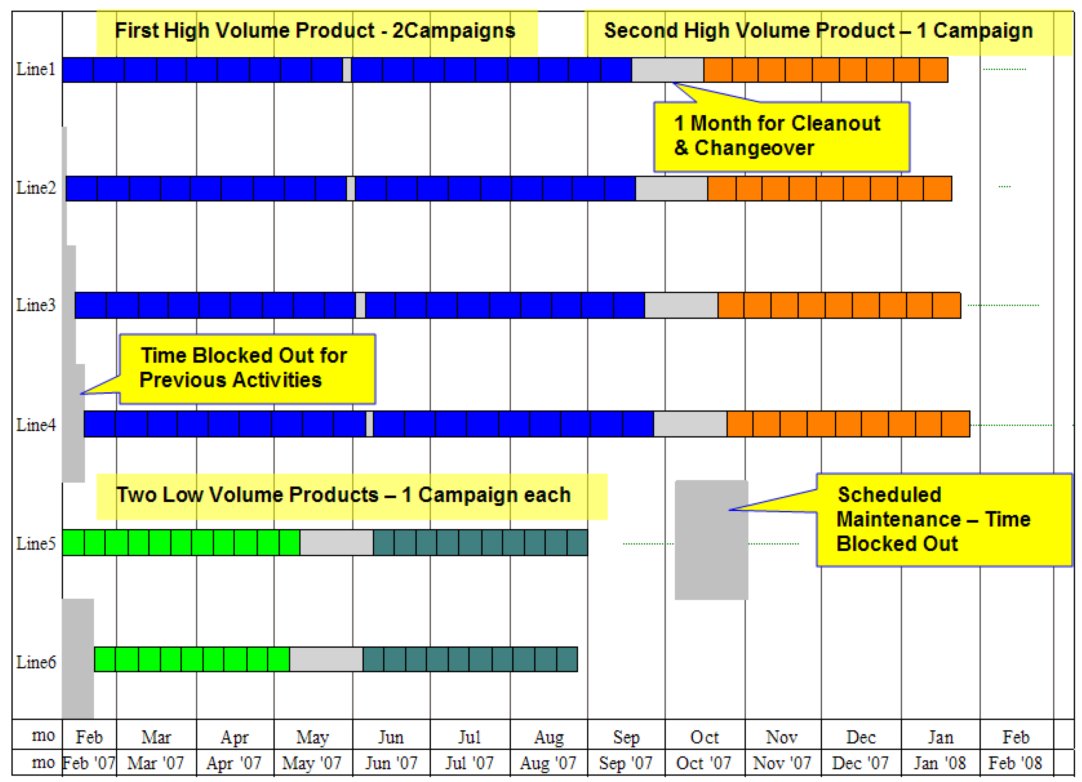
The objective of capacity analysis for strategic planning is to determine the best location to manufacture a set of products over a time horizon of a year or multiple years. The expected demand of a product is translated into a campaign of a certain number of batches for a specific production line. The overall effective cycle time of the process is used to estimate the occupancy of a line for a campaign. The results are visualized with Line Occupancy Charts (see
Figure 7). The various production lines are displayed on the y-axis and time on the x-axis. Delays for campaign changeovers and column repacking as well as line outages for preventive maintenance and holidays are taken into account. Campaign changeovers account for production line clean out and equipment adjustments required for accommodating the manufacturing of another product. Forecasts of product demand combined with capacity analysis facilitate capacity expansion decisions. If the available capacity cannot meet the estimated future product demand, a company must decide whether to expand capacity or secure capacity at a contract manufacturing organization (CMO). This type of high-level representation enables decision makers to have a bird’s eye view of their capacity needs in the coming years. The model can be easily updated on a regular basis to account for changes in estimated demand and events that affect available capacity.
Companies that purchase complex materials that have long lead times tend to use similar models for managing the ordering and supply of materials. By adding typical per-batch raw material requirements to the recipes, the demand for key raw materials can be calculated and visualized. A rolling 12-month plan is usually maintained. At the beginning of each month, this plan is updated by removing the completed batches of the previous month and adding the batches of the new 12th month. Furthermore, the current inventories of materials are updated and material orders during the coming month are determined.
Figure 7.
Line occupancy chart for capacity analysis and strategic planning.
Figure 7.
Line occupancy chart for capacity analysis and strategic planning.
3.4. Production Scheduling
Like capacity analysis, production planning and scheduling must consider the availability of plant resources in order to determine the time horizon for production of various products. However, the time horizon for production scheduling is generally much shorter than the time horizon for capacity analysis and long term planning. Furthermore, production scheduling models require a greater level of detail than capacity analysis models because they must allocate specific equipment items and other resources to the individual operations in each batch, and they must accurately capture scheduling interactions between these operations. This ensures resources are available when they are needed for a given operation within a particular batch. To facilitate adherence to resource limits, the model includes constraints, which are incorporated into the solution algorithm of the tool so that resources are not over-allocated.
In the sections that follow, a number of cases will be used to illustrate typical production scheduling challenges in biopharmaceutical plants that manufacture proteins using microbial fermentation. The concepts are equally applicable to cell culture facilities.
3.4.1. Recipe Overview and Schedule Generation
This example focuses on two proteins (Product-A and Product-B), which are produced by similar microbial fermentation processes. Both products are secreted in the fermentation broth. The upstream process consists of inoculum preparation in a small-scale seed fermentor followed by a production fermentor. The contents of the production fermentor are then transferred to a harvest vessel before centrifugation. The downstream process consists of centrifugation for biomass removal, followed by ion exchange chromatography (IEX), hydrophobic interaction chromatography (HIC), ultrafiltration-diafiltration (UFDF), and either freeze-drying (lyophilization) for Product-A or bulk filling for Product-B.
The production processes for Product-A and Product-B were modeled in a recipe-based scheduling tool called SchedulePro (from Intelligen, Inc., Scotch Plains, NJ, USA). SchedulePro, like SuperPro Designer, loosely follows the ISA SP-88 standards [
11] for batch recipe representation. A master batch or recipe for a process consists of one or more unit procedures. A unit procedure (“procedure” for short) is a distinct processing step that utilizes at least one primary piece of equipment for its entire duration. A list of the procedures included in this model, as well as the primary equipment units associated with those procedures, is given in the second column of
Table 7. There are two upstream lines, so each of the upstream steps has access to two possible equipment items. There is a single downstream line, so each downstream step is associated with a single equipment item.
Unit procedures may be further divided into operations (shown in the third column of
Table 7). Operations describe distinct sub-steps in a unit procedure. Furthermore, operations may utilize other resources such as labor, staff, materials, heating/cooling utilities, auxiliary equipment,
etc.
The relative timing of the various operations is determined by each operation’s duration and by scheduling relationships among operations. An operation’s duration may be fixed, rate-based (
i.e., dependent on the amount of material processed), inventory-dependent (
i.e., related to the time it takes for a storage unit to reach a specified level), or specified to be equivalent to the duration of another operation. Operations are not strictly required to be sequential within a procedure. They may overlap in time, or there may be delays between the end of one and the beginning of the next. The fourth column of
Table 7 shows the durations for each of the operations in the two microbial production recipes. Most operations have the same durations in both recipes. In cases where the durations differ, two specifications are listed in the fourth column of
Table 7.
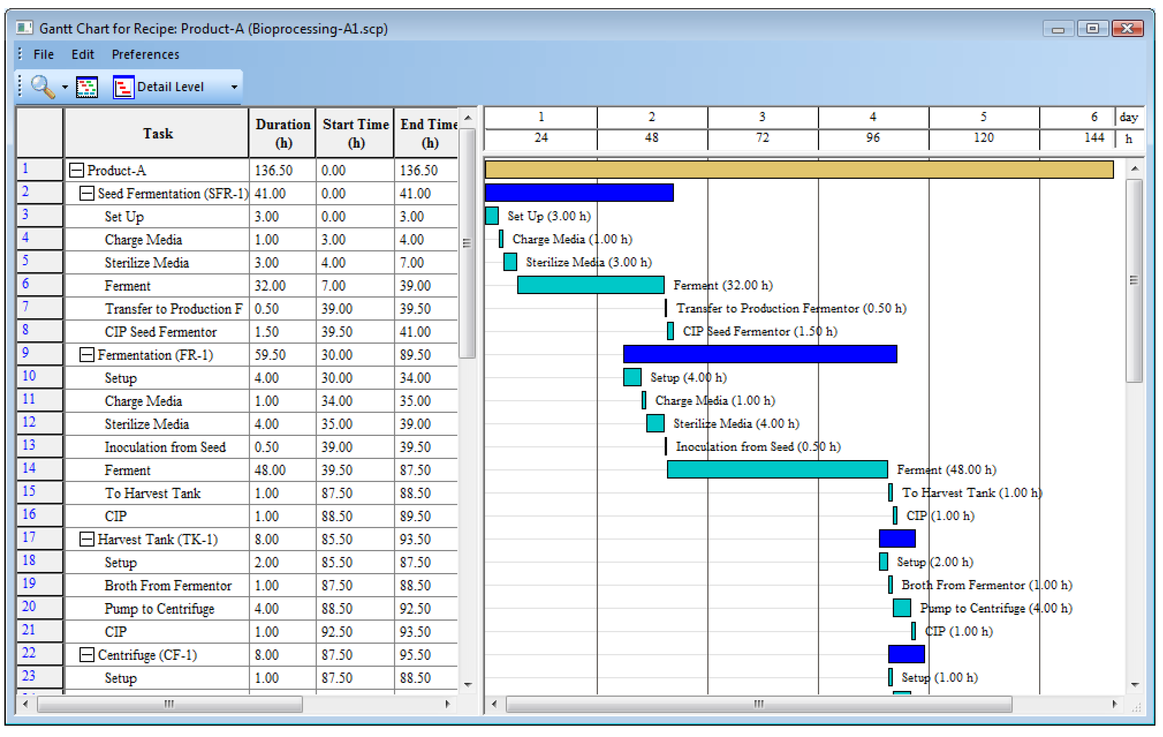
Once the recipe definition is complete, SchedulePro can translate the operation durations and scheduling links into a Gantt chart that enables users to visualize the batch process.
Figure 8 displays part of the Gantt chart associated with the Product-A recipe described in
Table 7. The light-brown bar at the top of the chart represents the duration of the whole Product-A recipe. The dark and light blue bars under the recipe bar represent the duration of each procedure and its associated operations, respectively. Each operation bar in
Figure 8 has a label to the right of it to identify the specific operation that it represents, and its duration is displayed in parentheses. The grid on the left-hand-side of the chart displays the same information in tabular form for the operations, procedures, and full recipe.
While the software can perform basic checks for completeness and consistency, the recipes should be validated using the Gantt chart and other outputs before they are used for generating production schedules.
A production schedule represents a specific plan that defines which recipes are executed when and with what resources. It is created based on production orders or campaigns. A campaign defines a request for a certain amount of product or a series of batches of a particular recipe. A batch represents the execution of a single recipe at a specific time and with specific resources.
Each campaign is given a release date representing its earliest start time as well as several scheduling options such as a due date or a start time relative to the start or end of some other campaign. In addition, the time between consecutive batch starts (cycle time) for a multi-batch campaign can either be fixed by the user or set to a minimum target value plus some user-defined slack time. Campaigns may also contain pre-production and post-production activities to account for time spent setting up or cleaning out equipment between product changes.
Table 7.
Operational data for Product-A and Product-B recipes.
Table 7.
Operational data for Product-A and Product-B recipes.
| Section | Procedure
(and Equipment) | Operation | Duration (h) Product-A/Product-B |
|---|
| Upstream | Seed Fermentation
(SFR-1, SFR-2) | Setup | 3.0 |
| Charge Media | 1.0 |
| Sterilize Media | 3.0 |
| Fermentation Ops | 32.0/24.0 |
| Transfer to Fermentor | 0.5 |
| CIP | 1.5 |
Fermentation
(FR-1, FR-2) | Setup | 4.0 |
| Charge Media | 1.0 |
| Sterilization Cycle | 4.0 |
| Inoculation from seed | 0.5 |
| Fermentation | 48.0/36.0 |
| To Harvest Tank | 1.0 |
| CIP | 1.0 |
| Downstream | Harvest Tank
(TK-1) | Setup | 2.0 |
| Broth From Fermentor | 1.0 |
| Pump To Centrifuge | 4.0/3.0 |
| CIP | 1.0 |
Centrifuge
(CF-1) | Setup | 1.0 |
| Centrifuge | 4.0/3.0 |
| CIP | 3.0 |
Pool Supernatant
(TK-2) | Setup | 2.0 |
| Receive Supernatant | 4.0/3.0 |
| Load INX column | 8.0/6.0 |
| CIP | 2.0 |
Ion Exchange
Chromatography
(C-1) | Setup | 3.0 |
| Column operations | 8.0/6.0 |
| Clean/Store | 2.0 |
Pool INX eluent
(TK-3) | Setup | 2.0 |
| Receive Eluent From INX Col. | 8.0/6.0 |
| Load HIC Col. | 6.0/4.0 |
| CIP | 1.5 |
Hydrophobic Interaction
Chromatography
(C-2) | Setup | 3.0 |
| Column Operations * | 6.0/4.0 |
| CIP Chrom Skid | 2.0 |
UFDF
(TK-4) | Setup | 2.0 |
| Receive HIC Eluent | 6.0/4.0 |
| UFDF (UF-1) | 4.0/3.0 |
| To Freeze Dryer/Bulk Fill | 0.5 |
| CIP | 1.5 |
Freeze Drying(A):
(LYO-1)
Bulk Filling (B):
(FL-1) | Setup | 4.0 |
| Transfer From UFDF | 0.5 |
| Freeze Dry(A) / Fill (B) | 24.0/4.0 |
| CIP | 1.5 |
Figure 8.
Recipe Gantt chart.
Figure 8.
Recipe Gantt chart.
Figure 9 displays a schedule that includes a campaign of six batches of Product-A (green bars) followed by a campaign of six batches of Product-B (brown bars). The inoculum preparation steps are not included in the chart. The white bars between the two campaigns represent product changeover activities that account for facility cleaning and equipment adjustments.
Figure 9.
Production schedule of two products with shared equipment.
Figure 9.
Production schedule of two products with shared equipment.
3.4.2. Accounting for Buffer Preparation and Holding
The recipes described in the previous section and the schedule displayed in
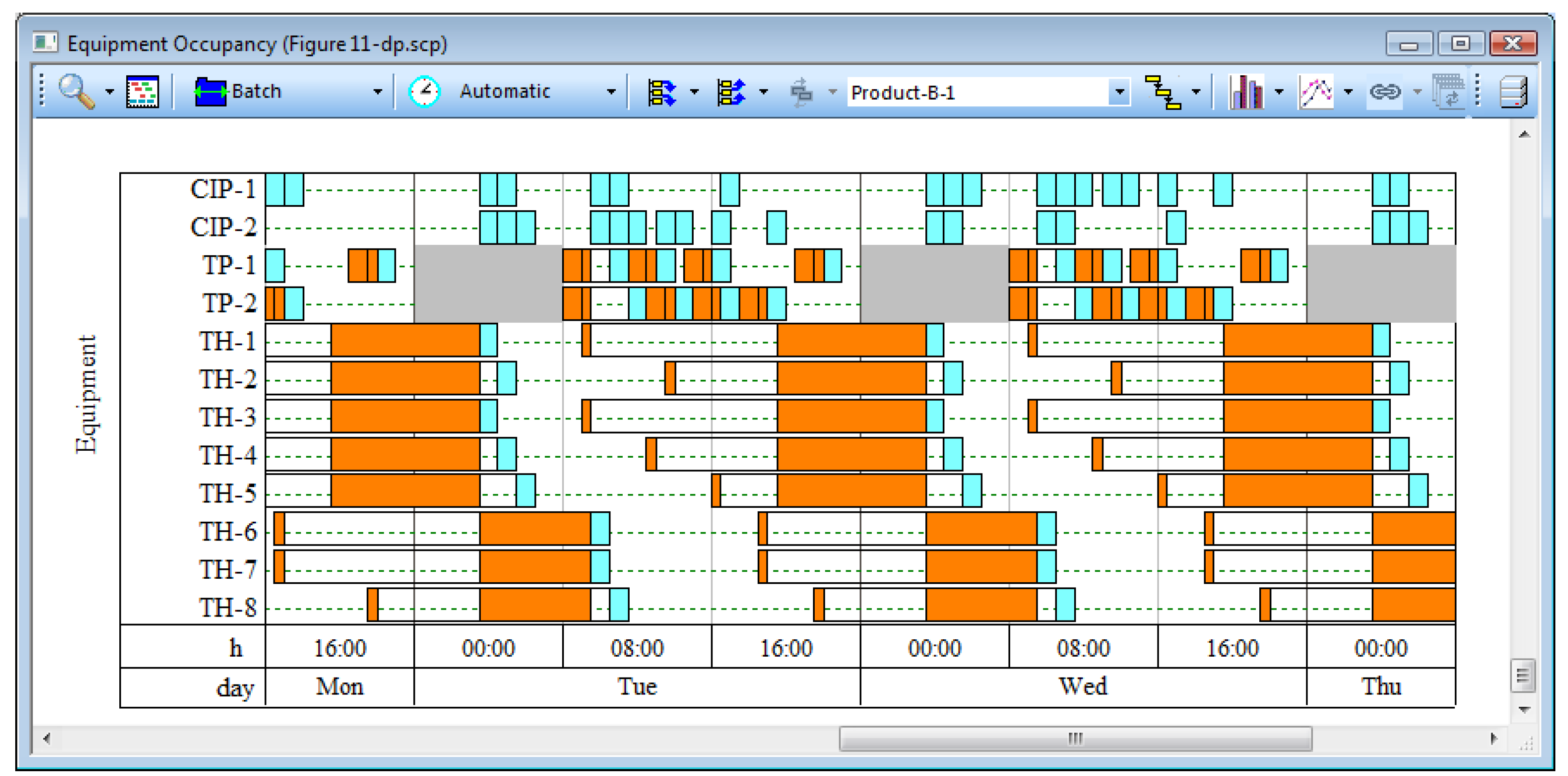
Figure 10 correspond to the main processing steps of Product-A and Product-B. However, typical biopharmaceutical processes also consume a large number of buffer solutions for the various product purification operations such as chromatography and membrane filtration. These buffers are typically comprised of dilute salt solutions, which are prepared in shared blending tanks and then stored in dedicated holding vessels. The transfer of buffers from the preparation to the holding tanks involves shared pipe segments and transfer panels, which act as switchboards to direct the buffers to the appropriate equipment. CIP skids are typically used to clean the equipment after use. Considering the above and the fact that a typical biopharmaceutical process requires more than twenty different buffer solutions, it can be easily understood why activities related to buffer preparation and holding contribute considerable operational and scheduling challenges to biopharmaceutical manufacturing.
Figure 10.
Scheduling of buffer preparation and holding activities.
Figure 10.
Scheduling of buffer preparation and holding activities.
For the sake of simplicity, this example assumes that each product requires only eight different buffer solutions (five buffers for the ion exchange chromatography operations and three buffers for the hydrophobic interaction chromatography operations). Each buffer is produced and consumed within a single batch. In cases like this, the buffer preparation and holding activities may be incorporated into the main process recipe. The extended recipes for Products A&B that include the buffer preparation activities are available in the literature [
16].
Figure 10 displays the buffer preparation and holding activities for two consecutive batches of Product-B. Cleaning activities are displayed in light blue color and processing activities in orange color. The top two lines represent the occupancy of the two CIP skids (CIP-1 and CIP-2), which are used for cleaning the preparation and holding tanks. Lines 3 and 4 represent the occupancy of the two shared preparation tanks (TP-1 and TP-2). Two tanks are adequate for making all eight buffers because the buffer preparation activities are relatively short, and using these tanks multiple times during a batch does not create bottlenecks as long as they are appropriately scheduled. Buffers are prepared during the morning and afternoon shifts only. The gray bars on lines 3 and 4 represent the downtime of the night shift.
Each of the buffers has its own dedicated holding tank (TH-1, 2, 3, 4, 5, 6, 7, and 8). The buffers are scheduled for preparation 12 h in advance of their use or as soon as possible thereafter when a preparation tank becomes available. This leads to considerable idle time for holding tanks between their “Receive Buffer” operations and their “Use Buffer” operations. However, this scheduling policy ensures that common delays in buffer preparation are easily accommodated and do not negatively impact the execution of the main process.
In this case, it was assumed that buffers are produced and consumed within a batch. Oftentimes, however, certain common buffers are prepared in larger quantities, capable of supplying multiple batches of a single process or even multiple processes at the same time. The preparation of such buffers is represented with separate recipes whose scheduling is driven by inventory control. The time-dependent consumption of such buffers is tracked by the model, and when their inventory level drops below a pre-set threshold, a new buffer preparation batch is automatically scheduled to begin. If topping off the holding tank is not allowed, two tanks are typically operated out-of-phase to hold such buffers (
i.e., when one supplies buffer to the process, the other is prepared to receive the next batch of buffer). Detailed information on how to manage buffer preparation based on inventory constraints is available in the literature [
16].
In most real processes, buffer scheduling is considerably more complex and challenging because of the larger number of buffers required for a typical process (more than twenty), the shared use of pipe segments and transfer panels, as well as constraints imposed by the limited availability of labor.
3.4.3. Considering Labor Constraints
In addition to providing insight into equipment constraints, multiproduct scheduling tools can facilitate understanding of shared plant resources such as labor, materials, utilities,
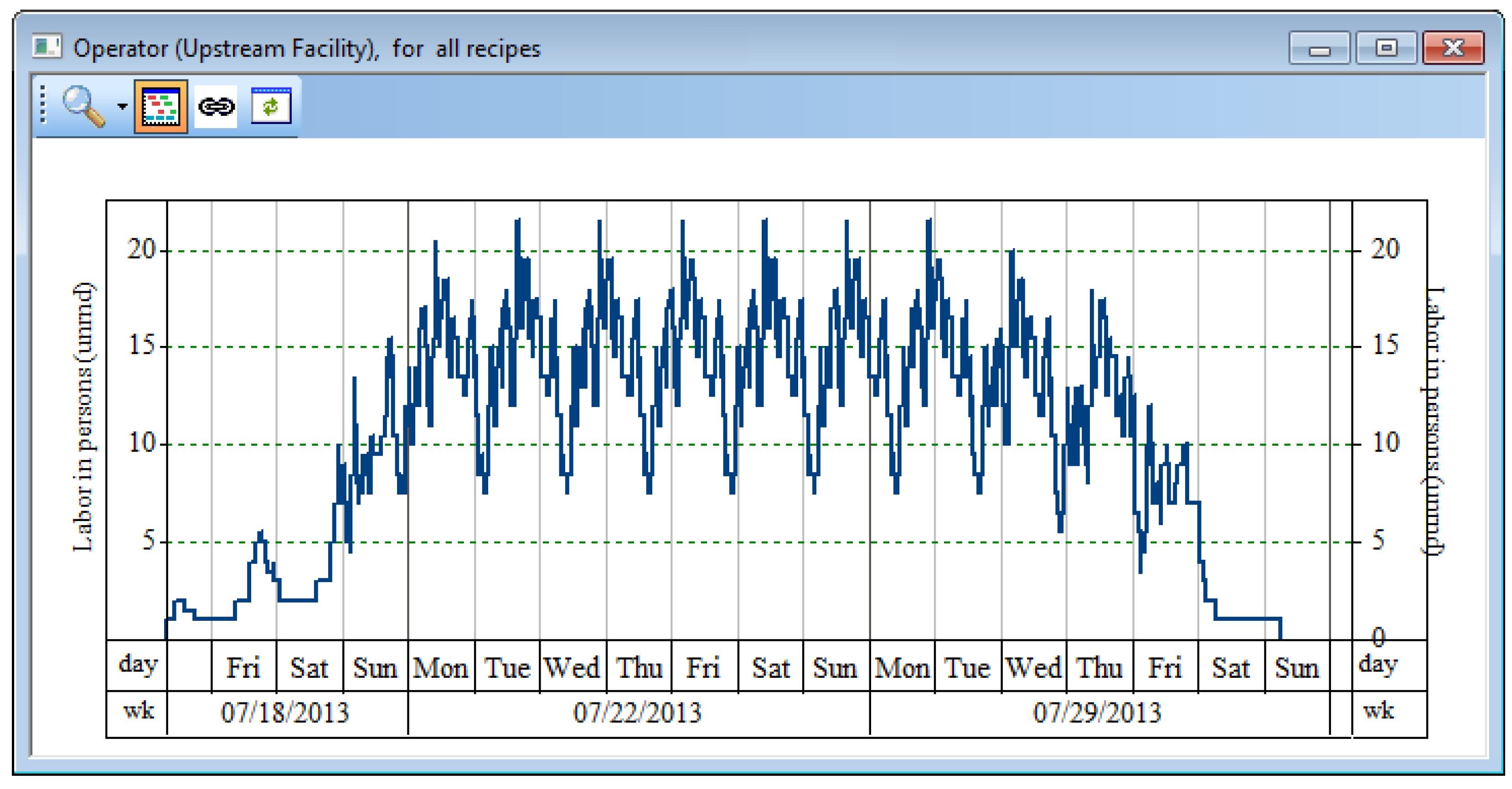
etc. This is important because in certain cases equipment constraints may not be the determining factor in production capability. Instead a lack of other resources may constrain production, and processing of one or more batches may be delayed as a result. This may result in decreased plant efficiency and throughput, and possible late orders. Therefore it is important to be able to anticipate process resource constraints and formulate strategies for dealing with them. Such strategies might include moving the start times of certain operations or adding extra short-term resource capacity. For instance, the total operator labor demand for the two campaigns described in the previous section (for Products A and B), is shown in
Figure 11. This chart was produced from the individual labor requirements assigned to each operation in each recipe. Note that in some cases a fractional labor unit was assigned to an operation since certain operations do not require constant action.
As
Figure 11 shows, there are large swings in labor demand over the course of a week. In this example, there is a low level of labor demand during the “startup” of these campaigns since initially only one batch of each campaign is being run. The demand for operator labor peaks when many batches are running simultaneously and when the operations occurring in those batches include many labor-intensive downstream processing operations. As shown in
Figure 11, the operator labor demand for this production schedule peaks at a maximum of 22 operators. If fewer than 22 operators are available, certain operations may need to be delayed. In some cases the delay of a particular operation will not delay the completion of a batch because the delay does not impact an activity on the critical path. In other cases the completion of one or more batches
will be delayed if a key operation is delayed due to labor unavailability. Plant scheduling tools can be utilized to anticipate periods of peak labor demand and to determine appropriate steps to ensure the plant can still meet its required production demands. For instance, it may make sense to have some operators work overtime, or to rearrange the scheduling of certain labor-intensive operations. Similar analyses can be performed for other resources, such as heating and cooling utility systems, purified water production,
etc. in order to avoid excessive use of a resource at any given time.
Figure 11.
Operator labor demand for multiple campaigns.
Figure 11.
Operator labor demand for multiple campaigns.
3.4.4. Production Tracking and Rescheduling
After a feasible production schedule has been generated, it must be regularly updated in order to incorporate new information. Real-world scheduling of batch plants involves a repeating cycle of the following activities:
Adding new batches to the current schedule
Updating the schedule to account for actual process information and adjusting for unforeseen events
Publishing the updated schedule
Many plant schedulers use spreadsheets to aid with these tasks, but spreadsheets can be difficult to update and maintain, and they often do not comprehensively account for complex dependencies between operations in multiple batches due to sharing of equipment and resources. Scheduling tools greatly reduce the effort required for tracking and managing these activities on a day-to-day basis.
One reason plant schedules must be updated regularly is the fact that schedules are based on average task durations, which are subject to variability. Differences between scheduled and actual durations may lead to resource conflicts with future activities. For instance, let us assume that the plant has begun running the production schedule displayed in
Figure 12. This chart displays the schedule for campaigns of two different products (A & B) running on two different production lines. The two lines share a centrifugal separator (CF-1) and two CIP skids (CIP-1 and CIP-2). Suppose that about 5 days have elapsed since the start of the first batch. The red vertical line during the morning of Tuesday 7/23/2013 represents the “current time”. The current time line results in the division of activities into three categories: completed (displayed by a crossed hatch pattern in the chart), in-progress (displayed with a diagonal hatch) and not-started (displayed with a filled pattern).
Figure 12.
Scheduling conflicts due to a delay.
Figure 12.
Scheduling conflicts due to a delay.
Let us assume the fermentation operation in batch “Product-A-1-2” (the second batch of the Product-A campaign that utilizes the top line) took 8 h longer than planned. As a result, the third batch of the Product-B campaign (Product-B-1-3) has a conflict with the second batch of the Product-A campaign in centrifuge CF-1. This conflict is displayed in
Figure 12 with a new line on the equipment occupancy chart directly below line CF-1 (this new line is labeled with an exclamation point and the conflicting procedure associated with batch B-1-3 is circled on that line). The delay in the fermentation also causes a conflict with the freeze drying of Batch A-1-3 (this conflict is shown on the line labeled with an exclamation point immediately below LYO-1, and the conflicting freeze drying procedure is circled.) In other words, a delay in a single operation (the A-1-2 fermentation) creates conflicts with two other batches in two different equipment units.
At this point, the next logical step is to resolve the conflicts created by the initial delay. The scheduling tool first attempts to resolve conflicts by utilizing alternative resources. If no alternative resources are available, conflicts are resolved by delaying the start time of the conflicting activities. Such delays may cause new conflicts, which are resolved recursively until all conflicts are eliminated. The scope of conflict resolution is controlled by the user. The tool can automatically resolve conflicts for a specific batch, a campaign or the entire schedule. Alternatively, the user also has the option to manually resolve conflicts by dragging and dropping activities directly on the chart.
Since schedules must be regularly updated to account for variations in process times, addition of new batches, etc., contemporary scheduling tools are equipped with databases (typically SQL Server or Oracle) for tracking the status of production as a function of time, communicating the data to various stakeholders, facilitating updating of the data, and archiving the information about completed batches and campaigns. A variety of reporting tools are available for viewing data stored in SQL Server and Oracle databases. These reporting tools facilitate creation of customized views for the various stakeholders. For instance, detailed views that focus on the activities of a specific production line for a specific date or shift are useful for providing execution instructions to operators and line supervisors. Specification of actual start and completion times and documentation of deviations might be done through the same views. Additionally, dashboard views and reports, which summarize high-level information, can be generated for executives and viewed through browsers and smart phone applications. This enables production managers to monitor the status of campaigns and projects remotely on an on-going basis.
In addition to storing historical data and tracking the status of production, central databases facilitate communication with enterprise resource planning (ERP) and automation tools. For instance, an ERP tool might deposit a new work order in the database. The order might then be imported into the scheduling tool, scheduled, and executed. The status of the order, along with information on consumption and generation of materials, can be communicated back to the ERP tool from time to time. This workflow facilitates comprehensive production planning, scheduling, and inventory management and provides access to the key production data to all stakeholders in the company. Communication with automation tools facilitates the updating of the status of execution of the various operations of a batch.
Schedule tracking bears some similarity to batch record maintenance. Many manufacturers use electronic batch record (EBR) systems to maintain a manufacturing log of each batch. Such systems may be subject to regulations such as 21 CFR Part 11. This regulation sets standards to ensure that any changes to the records are made by authorized individuals and are fully traceable. Normally a scheduling system is a forward-looking tool, but the plant scheduler may also use EBR data to maintain the schedule.
3.5. Facility Design and Debottlenecking
While capacity analysis asks the question “How much can I produce in a given period of time with the resources that I possess?”, facility design asks “What resources will I need in order to meet an expected production rate?” This question can be answered by using the scheduling tool to model the expected production scenarios and to determine the required types and quantities of relevant resources (equipment, utilities, etc.).
Similar models are used when debottlenecking existing facilities. Oftentimes, the production objective of an existing plant can be met through optimized scheduling without adding any additional resources. This may be accomplished using the same types of production scheduling activities described in the previous section. Other times it will be necessary to add additional resources (equipment, labor, utilities, etc.) in order to eliminate the plant bottlenecks and meet the new production objectives.
To illustrate the steps required for facility design and debottlenecking, the rest of this section will focus on sizing of utility systems and more specifically on systems that supply purified water to biopharmaceutical facilities.
3.5.1. Sizing of Utility Systems
Biopharmaceutical plants utilize purified water of multiple grades, such as reverse osmosis (RO) and water for injection (WFI). Purified water is used for media and buffer solution preparation, equipment cleaning, steam generation, etc. RO water is generated by passing well or city water through a combination of column adsorption and membrane filtration units. WFI is generated by distilling RO water. Both systems include a generation unit (or train), a storage tank, and a recirculation loop that supplies material to the various operations that need it. A methodology for sizing such systems in a systematic way is presented below.
The sizing of a water system involves a trade-off between the size of the holding tank and the capacity of the generation unit (e.g., a still in the case of WFI). The minimum still size corresponds to the average overall WFI demand over an extended time period. However, the use of the smallest still capable of meeting average plant demands results in a very large and expensive holding tank in order to even out fluctuations in WFI demand. It also leads to significant water losses during loop sanitization shutdowns, and it cannot accommodate any plant expansions that would increase average WFI usage. A better approach is to use a larger still combined with a smaller tank whose sizes can be derived from water demand charts.
Figure 13 displays such a chart that corresponds to the production scenario shown in
Figure 12. The black lines on
Figure 13 represent instantaneous WFI demand and they correspond to the y-axis on the left-hand-side. The blue lines represent averaged demand for 8-h intervals and they correspond to the y-axis on the left-hand-side. The green lines represent cumulative demand for 8-hour intervals and they correspond to the y-axis on the right-hand-side.
Figure 13.
Water For Injection (WFI) demand chart for utility sizing.
Figure 13.
Water For Injection (WFI) demand chart for utility sizing.
Figure 13 includes enough information for sizing all three elements of a WFI system. The tallest black peak (roughly 17,000 L/hour) provides useful information for sizing the circulation loop, since the pumps and the pipe diameter of the loop must be able to accommodate the highest instantaneous flowrate plus any other constant loads on the system. The tallest green peak provides useful information for sizing the storage tank. In this case, a storage tank of around 47,000 L would be required. The tallest blue line peak provides useful information for sizing the still. In this case a still capable of producing around 6000 L/hour would be sufficient. As mentioned previously, there is a trade-off between tank size and still rate. This trade-off can be visualized by changing the averaging period associated with this chart. A longer period associated with average and cumulative demands results in a smaller still size but a larger storage tank.
Figure 14 displays the operation of a WFI system based on the capacity parameters determined from
Figure 13 (
i.e., 47,000 L tank capacity and 6000 L/h still rate). The green horizontal line at the top of this chart corresponds to the 47,000 L storage tank capacity. The dark blue line represents the inventory of WFI in the storage tank. The thin black line represents the rate of WFI consumption by the two production lines that utilize the system. Finally, the light blue line shows the operation of the still, which is turned on (producing 6000 L/h of fresh WFI) when the level in the tank drops to around 80% of its capacity and off when it reaches 95% of the tank’s capacity. This line also represents the material being drawn from the RO system (conversion losses are accounted for by specifying a conversion factor). This is a case of “cascaded” water systems, since RO water is used to produce WFI. The RO system may be designed using the same technique that was described above. Recall that RO water is used for WFI production as well as directly in the process. As a result, it has a greater overall consumption than WFI, and there are many times when the discharge from the RO water tank is much higher than the simultaneous supply into the WFI system. Therefore the RO system requirements may be very different from those of the WFI system.
Figure 14.
WFI system operation.
Figure 14.
WFI system operation.
Another important consideration related to WFI systems is the need for periodic sanitization of the system, which involves shutting down the entire system for cleaning, including the storage tank. Consequently, loop sanitization should be scheduled during periods that do not include operations requiring fresh WFI.
The above methodology can be used for sizing any storable utility. For instance, in steam generation systems, the steam accumulator plays the role of the storage capacity. In contrast, the sizing of non-storable utilities (e.g., electric power) must be based on the highest instantaneous demand. If the maximum expected peak is too high (e.g., due to several overlapping operations that consume electric power), the schedule should be modified to reduce overlaps of such operations and lower the highest expected instantaneous demand.
4. Conclusions
Process simulation and production scheduling tools can play an important role throughout the life cycle of process development and product commercialization. In process development, simulation tools are becoming increasingly useful as a means to analyze and evaluate process alternatives. When transitioning from development to manufacturing, simulation models enable efficient technology transfer and process fitting. In manufacturing, production scheduling tools play a valuable role by generating feasible production schedules and enabling manufacturing personnel to efficiently handle process delays and equipment failures. Such tools also facilitate capacity analysis and debottlenecking tasks.
The biopharmaceutical industry has only recently begun making substantial use of advanced process simulation and scheduling tools for process design, analysis, and improvement. As these tools continue to improve, and as additional industry practitioners become proficient with them, the use of these technologies is expected to increase. In the future, we can also expect to see tighter integration between these tools and other enabling information technologies, such as supply chain tools, manufacturing execution systems (MES), batch process control systems, process analytical technologies (PAT), etc. The result will be more robust processes and efficient manufacturing leading to more affordable biological products.


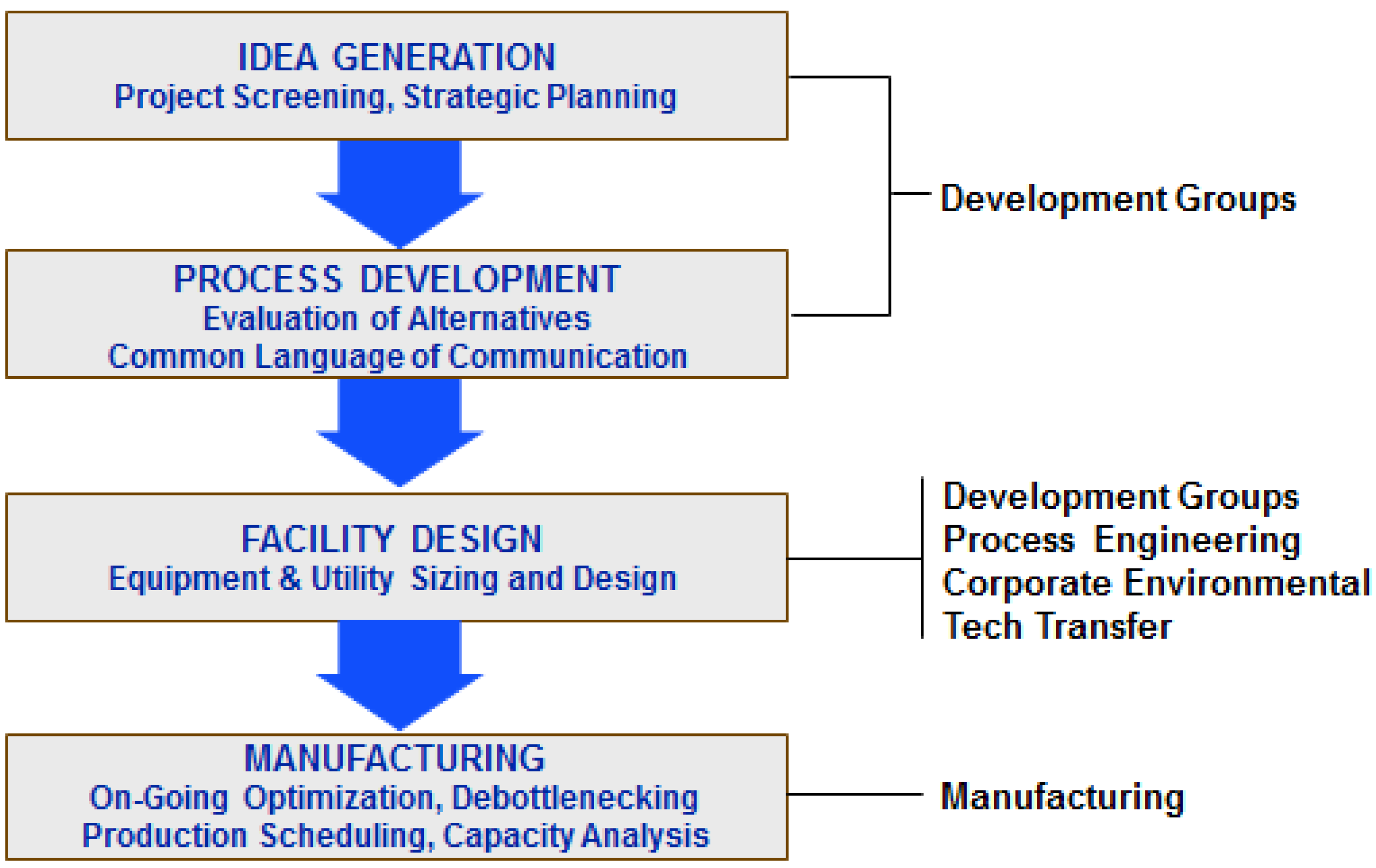
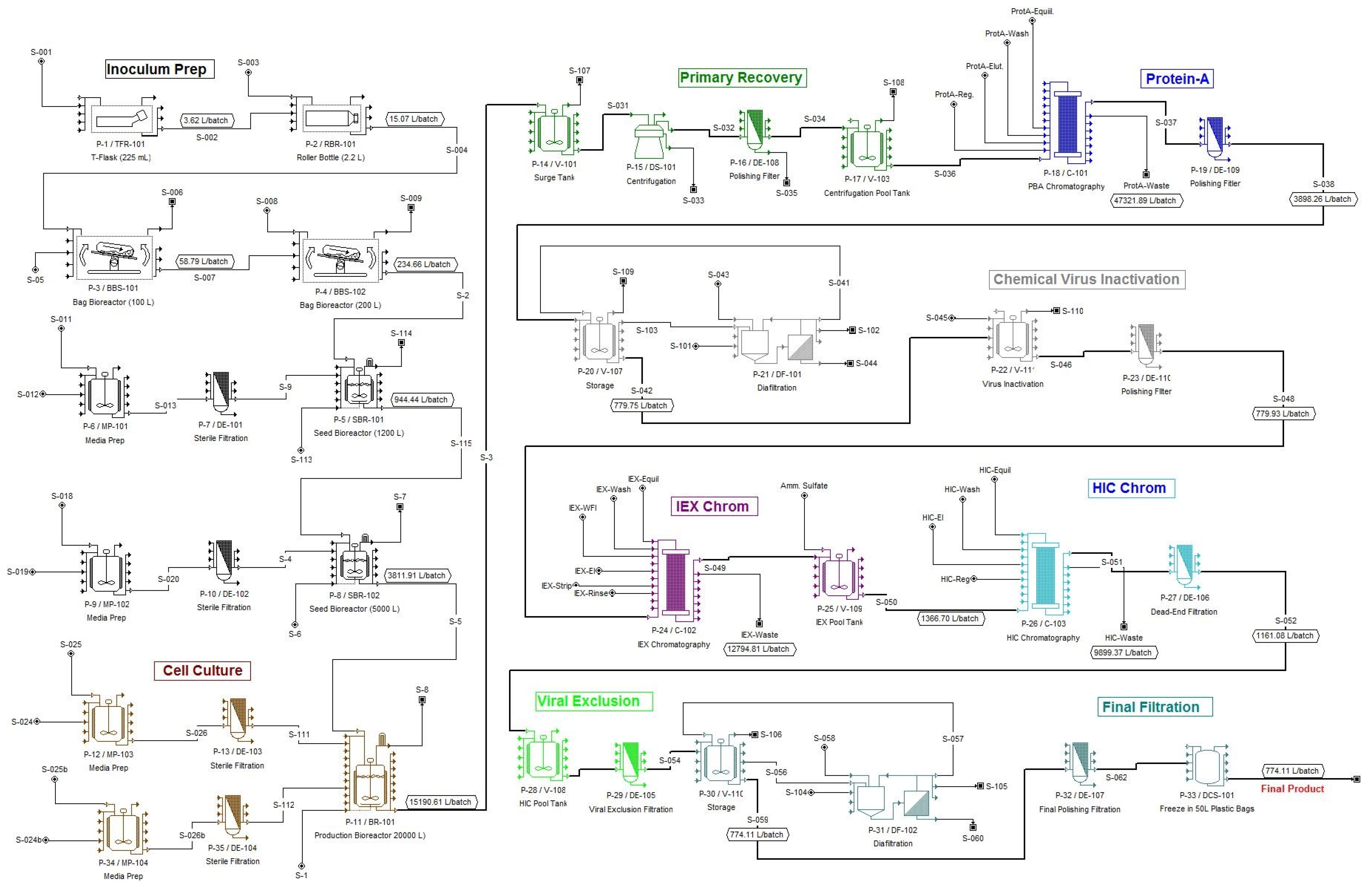

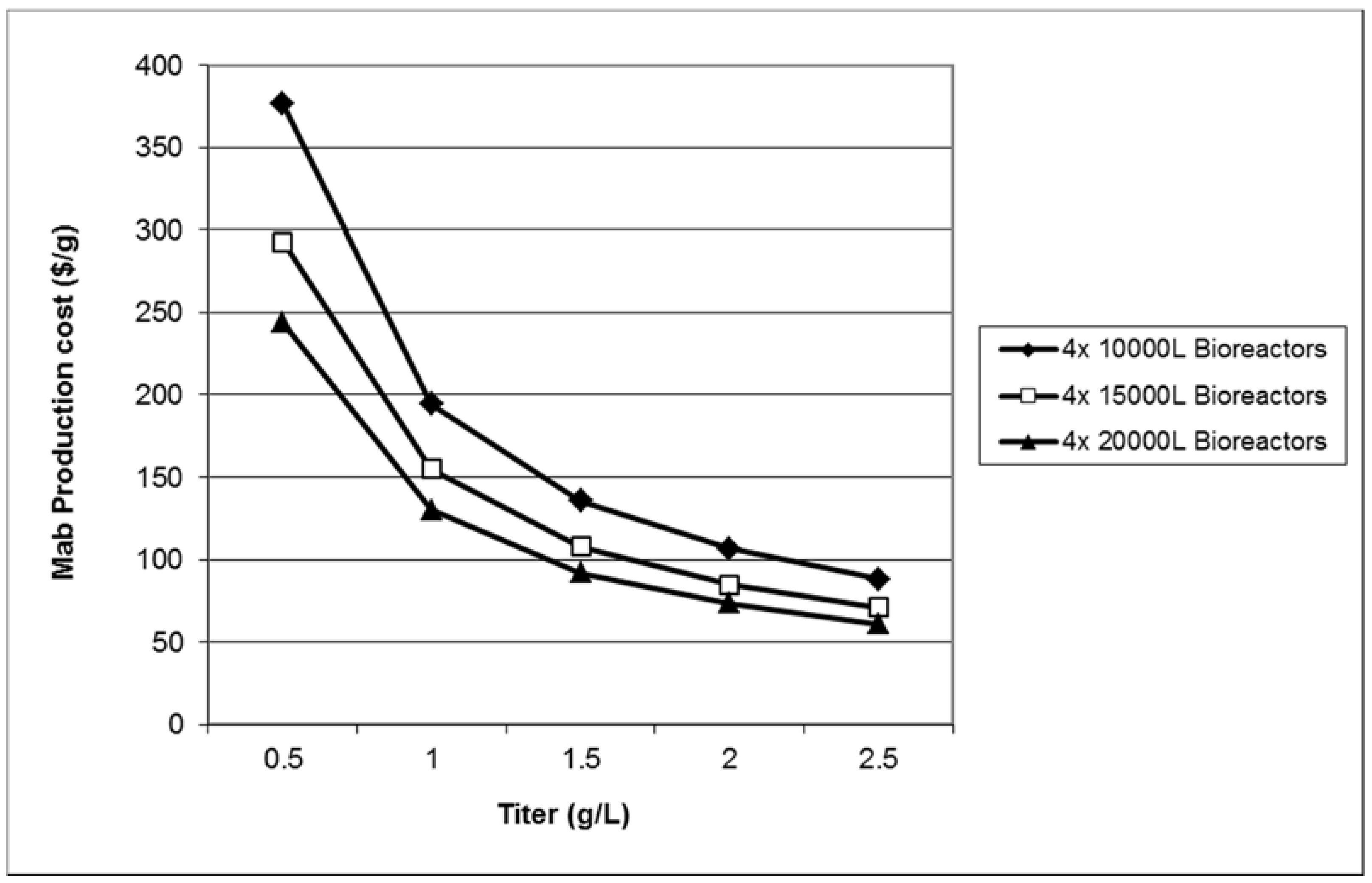
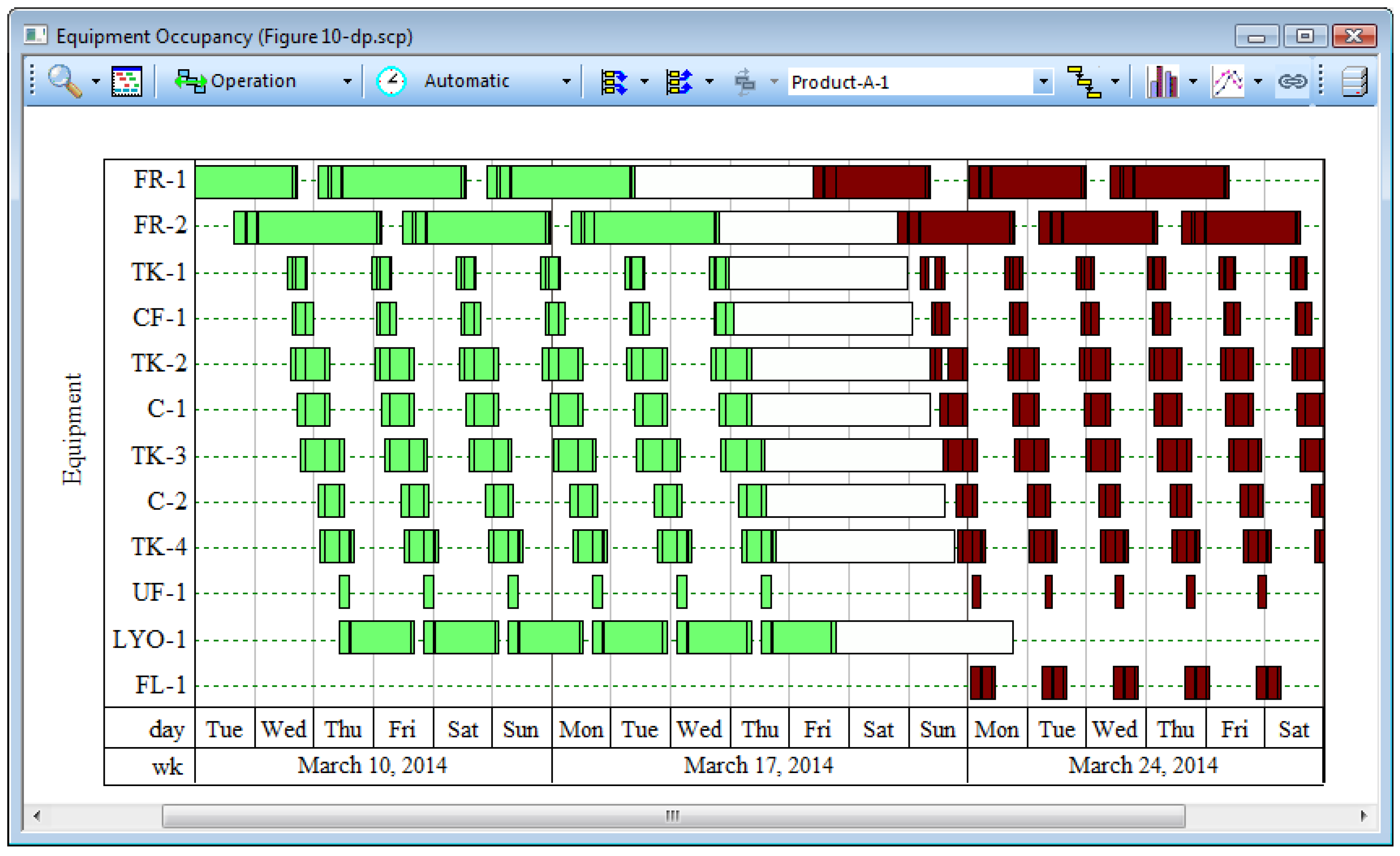
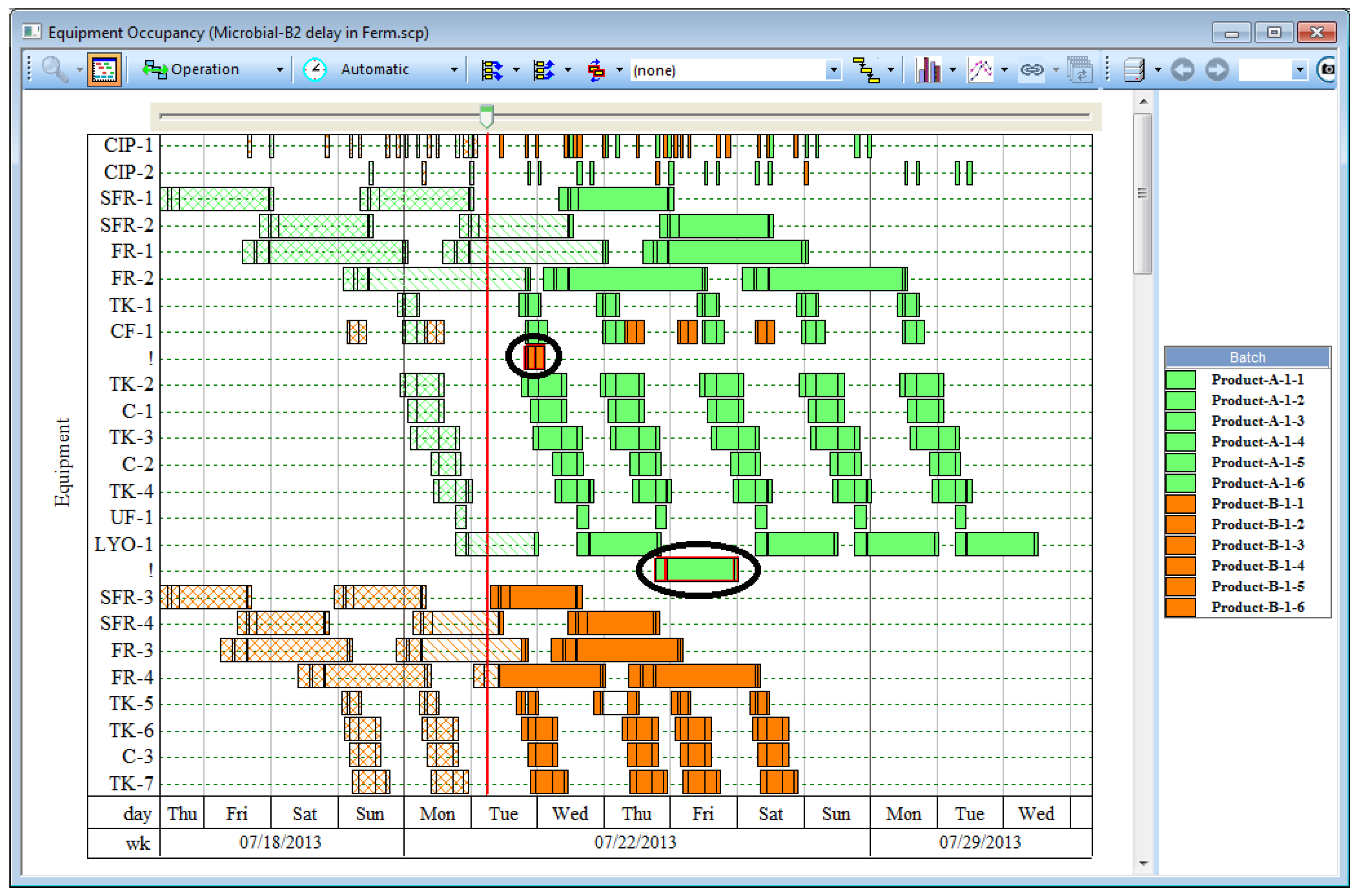
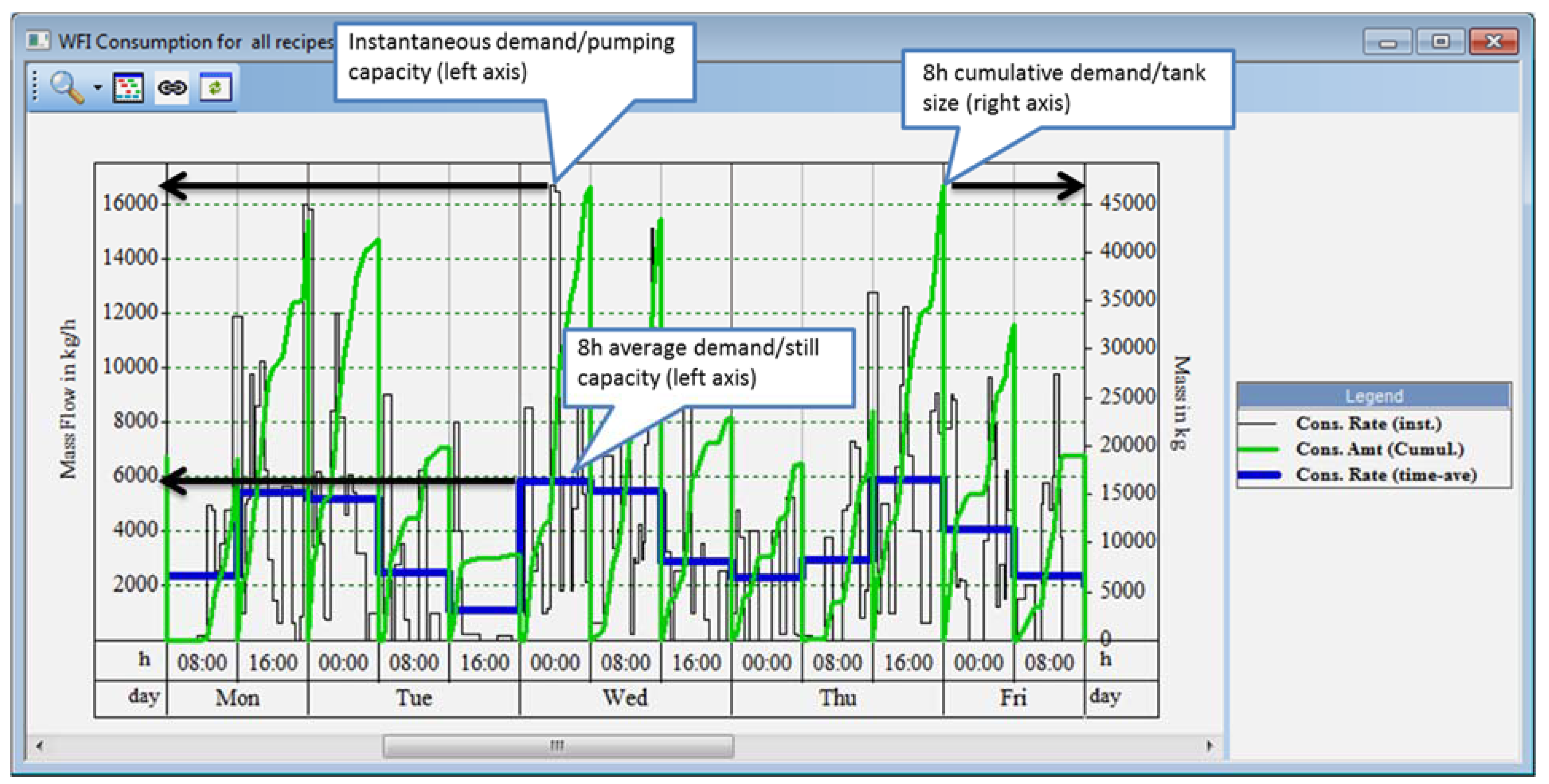
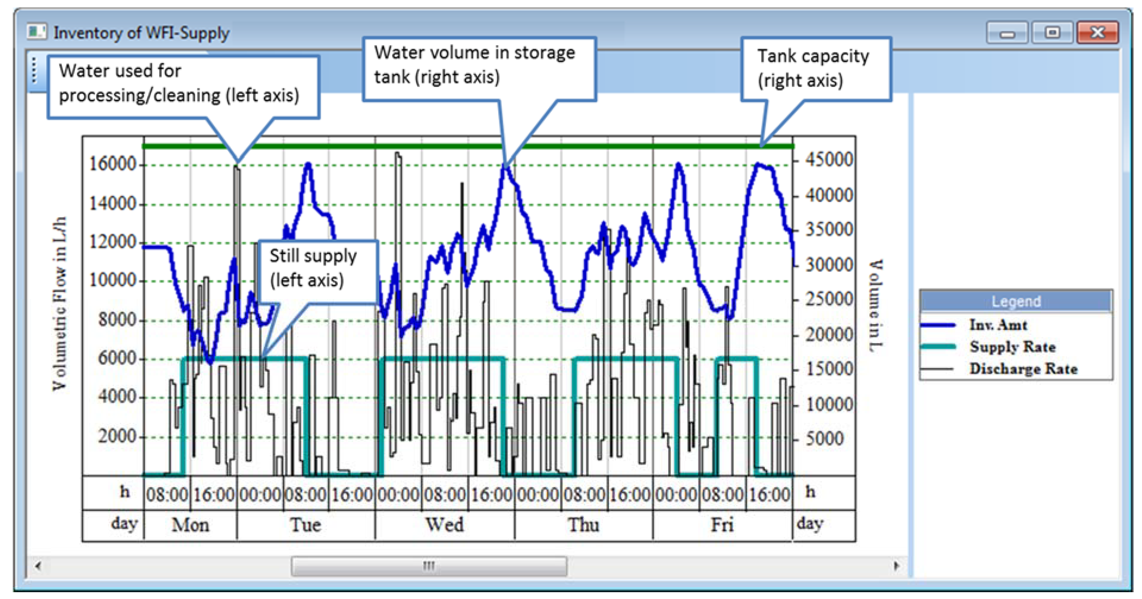