1. Introduction
The main motivation for studies on plants’ water use and the relationship with water stress is to optimize water management. Quantifying the total water flux from vegetated surfaces to the atmosphere or evapotranspiration (ET), and separating it into the components, transpiration (Tr) and soil evaporation (Es), is important for hydrology, land use and water use analysis. Studies on water flux contribute to understanding and help to mitigate the impacts of climate and land cover changes [
1]. Estimating crop water requirement is necessary for water resource planning and for efficient use of irrigation water.
According to worldwide surveys, over 70% of the world freshwater resources are consumed in irrigation and agricultural practices [
2,
3,
4]. Consequently, reductions in irrigation water use have a high impact on the availability of water for local or downstream users. Definitions of irrigation efficiency have been discussed [
5], and the lack of efficiency at different steps of water delivery processes (e.g., on-farm and conveyance efficiency) can account for important losses. Apparent inefficiencies in traditional irrigation sometimes result in a recharge of water courses and local water tables. In fact, ecological benefits are sometimes not adequately considered in analyzing irrigation water uses.
The economy of on-farm water use is directly linked to energy savings, when using pressurized irrigation, and agrochemical savings in general. When the irrigation is expensive, farmers are interested in optimizing water application efficiency. When water quality is problematic, saving water is related to groundwater environmental protection since it is difficult to revert water quality degradation [
6].
Irrigation is vital for achieving sustainable levels of crop growth and economic yields whenever precipitation is too low to meet crop water needs. In Mediterranean climates, the expected summer water scarcity and rainy winter usually lead to dominant stands of deeply-rooted woody plants because they can extract deep water from winter recharge, and they are better able to withstand summer water deficits. These aspects are discussed in
Section 2, where a paradigmatic example illustrates a dependence on irrigation for Mediterranean climatic conditions and the dominant land use of woody crops.
Irrigation issues cannot be disconnected from geographical, environmental, social and food safety concerns. The history of the relationships between agriculture and nature [
7], in which the history of irrigation is included (e.g., [
8]), are tools to consider in an analysis regarding a general discussion of irrigation benefits, enabling one to understand the present to prepare for the future, an analysis that is out of the scope of this work. In several countries having summer water scarcity, it is recognized that the investments in irrigation infrastructure have increased temporal and spatial water availability during summer. For example, the Alqueva dam (Portugal), which is the largest artificial lake and “the most modern construction of its kind” in Europe [
9], has promoted a more economically sustainable agriculture in the area.
This composition deals with irrigation scheduling only at the plot level and emphasizes the specific requirements/problems of woody crops in Mediterranean-type climates under water stress. The classical approach for scheduling is the “water balance method” that uses estimations of ET. Due to uncertainties of ET models, many researchers have proposed a so-called “alternative method” that uses a plant-based water status approach [
10]. Actually, the approaches are not seen here as true alternatives, but rather as potential complementary tools.
This composition does not aim to develop ET models or to provide crop coefficients’ or water status indicators’ analyses more than necessary for its aim. These topics are developed in specific reviews of this Special Issue. Before entering into central aspects of the methods, we briefly present background information, with the following structure: the context of Mediterranean climates, the ability of deeply-rooted woody plants to withstand extreme water deficits, why dependence on irrigation increases in such edaphoclimatic (soil and climate) conditions (
Section 2), the need for estimating ET for planning and scheduling irrigation, by using simple models (
Section 3), and the importance of quantifying stress in woody crops (
Section 4). The next sections require a previous description of the basic irrigation concepts and assumptions, to introduce nomenclature and perspectives, with emphasis on the component to quantify water stress (
Section 5).
Section 6 describes our perspective of the so-called ET based (feed-forward) and plant based (feed-back) approaches to schedule irrigation, not as alternatives, but as potentially complementary. Simple approaches to model ET under stress (stress functions) are discussed and justified (
Section 7). Several examples are given on stress coefficients in woody crops (
Section 8) to inform the discussion and illustrate the importance of appropriate stress functions in simple ET models (
Section 9). Arguments are given for the combined use of these two approaches serving a self-learning perspective (
Section 10) to be further developed in future work. A few final remarks conclude (
Section 11).
2. Consequences of a Mediterranean Climate: Why Do Woody Plants Adapt Better?
Mediterranean soils tend to be shallow with low organic material content due to the fluctuation between humid and dry conditions. As a result, there is a greater need for irrigation, especially on high slopes of fragile soils that are subject to erosion.
Portugal is a country with a high contrast in water availability between seasons, and the dependence on irrigation is discussed in a geographical perspective by Ribeiro [
11,
12] and Ribeiro et al. [
13]. The temporal heterogeneity of precipitation is high, with about 70% of the annual precipitation falling in six months (autumn/winter), and is low when evapotranspiration demand is high. This precipitation trend is a specific feature of all regions with a Mediterranean-type climate (6% of the world land). This fact introduces a strong disequilibrium between water availability and demand in summer, but in addition, the summer crop water requirements are higher than in most areas occupied by man. This is attributed to the high levels of summer solar radiation and passing of hot, dry air masses due to the reduced evaporation from dry surfaces. This is aggravated in areas with higher wind speed. In areas with undulating terrain and steep slopes, high yearly water losses by runoff are observed, e.g., 385 mm in Portugal [
14]. The high levels of runoff lead to erosion hazards that largely determine the extremely shallow soils in many Mediterranean areas.
In conclusion, despite 67% of the land (Portugal) being covered by woody plants, mainly forests, soil erosion is a serious problem, as in many areas of Southern Europe [
15]. The soil water storage in such conditions reaches extremely low values in most areas due to its texture, poor organic material and shallow depth. Because there is limited soil water storage capacity, there is a high dependence on irrigation during the dry season.
Spatial heterogeneity of precipitation in Portugal is extremely high: according to data from the Instituto Português do Mar e da Atmosfera (IPMA) [
16], the yearly average precipitation (about 900 mm) ranges from >2800 mm in the northwest (NW) of the country to <600 mm in the south, with almost an inverse relationship for mean temperature distribution (5.4 °C in winter to 18.0 °C in summer). The ratio between total water availability and water demand for human uses (excluding ecosystem services) is on average 5.3 in Portugal, but varies from 75 in the NW to 0.7 at the southern coast. This distribution of water availability reflects the fact that poor soils and restrictions in available water in some areas [
17] have historically limited agriculture. In Portugal, as in many other countries, water availability seems related to statistically observed asymmetries in population density. This statement seems to be generally valid for SW Europe, i.e., the Iberian Peninsula, as well as for SE Europe (e.g., Greece): in the driest areas of Portugal, the population density is as low as seven inhabitants/km
2 [
18]. In fact, the average number of inhabitants/km
2 in these southern countries is lower than the European average (113 inhabitants/km
2). In addition to the water availability problem, frequent cycles of drought make it even more difficult to ensure stable water sources for all regions. Rainfed woody crops are traditional in some areas, but not dominating in economic terms. For economic sustainability, irrigation is often mandatory. Although, low crops generally require more water than woody crops, there is a recognized need for efficient use of water in orchards and vineyards via deficit irrigation (DI).
In conclusion, woody crops are especially well adapted to sustainable rainfed agriculture or deficit irrigation (DI) in a Mediterranean climate. Basic irrigation concepts and the role of ET in irrigation scheduling will be briefly summarized with emphasis on the aspects that are critical for woody crops.
3. Need for ET Data and Simple ET Modelling Approaches in Irrigation: Stress Coefficients in DI
Evapotranspiration data are needed for scheduling irrigation, but also for planning and other applications. Emphasizing the requirement for simple modelling of ET approaches and the inclusion of stress coefficients in DI applications is the motif for a brief narrative aiming to frame how traditional solutions appeared and what their limitations are for woody plants (developed in
Section 4).
Irrigation planning projects require information on ET to determine (1) how much area can be irrigated and (2) to plan the water delivery network and the pumping system. Quantifying crop water requirements is respectively necessary for (1) the complete vegetative cycle and (2) the period of highest consumption. For planning, a time series is used to perform a statistical analysis, select a specific probability of occurrence that is consistent with the investment and expected added values and risks.
Direct measurement of ET faces limitations in small fields and/or woody crops. The applicability of micrometeorological or hydrological methods has been described often (e.g., Ferreira et al. [
19]). Due to such limitations, up-scaled measurements of water use of individual plants with sap flow methods (SF) are an alternative to quantifying Tr at the plot level, but several studies suggest problems can arise concerning the ability to deliver good absolute values, when compared to data from the eddy covariance (EC) micrometeorological method or other common methods. If a complete soil water balance is not feasible (due to rooting depth or sparse roots), a combination of SF and EC methods is useful for providing reliable long-term (whole season) ET data series [
19,
20,
21]. Data used for the examples that follow were mostly obtained by this robust methodology.
Measuring ET requires expensive equipment and know-how, and it only provides real time data, which are not enough for irrigation planning. Long-term and good quality ET measurements are required for model validation. However, the model outputs are often unsatisfactory for woody stands at this time.
Models are applicable to any step in the soil-plant-atmosphere continuum. Well-known physically-based models are applied between stomata and a reference level in the atmosphere above the canopy. Those models require meteorological data inputs, the bulk aerodynamic conductance (g
a), the bulk stomatal conductance (g
s) or canopy conductance (g
c), physical constants and crop parameters (e.g., albedo). A well-known example is the Penman-Monteith (P-M) equation [
22], which added g
c to the Penman equation [
23]. Both the Penman and P-M equations use a “single-leaf” assumption (i.e., the canopy surface is similar to a large single leaf).
Using meteorological data is convenient for planning because agrometeorological networks are available worldwide, and historical records for statistical analysis are usually available. This notwithstanding, g
c values are not well known, and they are not easy to determine for real-time use. To solve this problem, the idea of using a reference crop ET, where the ET is relatively independent from stomata opening, was developed. This is true for a low height vegetative stand that is as smooth as possible (high omega factor, as described in
Section 4) and not limited by water availability.
This concept is often attributed to Thornthwaite [
24] who presented it as potential ET, with the reference being a healthy, fully-soil-covering, well-irrigated grass crop with standard height. ET for the reference crop was later called reference ET (ETo). Many lysimeters with grass in reference conditions were built, for selecting the so-called reference (potential) ET equations. Such equations [
25,
26,
27] generally had increasingly broader adequacy as the number of input variables increased (as in [
23]). Due to limitations in the availability of meteorological variables, for decades, several simplified equations were proposed and compared with ETo measurements (historically lysimeters with grass) to check local validity [
28]. In general, restricted availability of input variables restricted the validation of simplified ETo equations. The use of the P-M equation with a predefined parameter for g
c and an inverse function of wind speed for g
a to estimate the ET from a broad expanse of 12 cm-tall vegetation, that is not water limited, was later proposed and re-written for easy application on a daily or hourly basis [
29,
30].
Energy-limited crop ET (ETc) occurs from a crop when there is no reduction in ET due to water or other stress factors, so it corresponds to the maximum or potential ET for the crop considered. To determine ETc for a specific crop and climatic conditions, the classical approach is to multiply ETo by a crop coefficient (Kc) value for different periods of the crop season. Doorenbos and Pruitt [
26] and later Allen et al. [
29] presented tables and described procedures to obtain Kc, based on numerous previous studies (e.g., [
31]). These Kc values are not only dependent on crop and stage of development, but also on agronomic practices, such as spacing. Often, Tr becomes the most important term in ET because excessive Es losses are avoided by well-adapted irrigation techniques or cultural practices. The use of a single Kc must then consider the conditions at the soil surface, depending on wet fraction and occurrence of irrigation events. Earlier studies also indicated that the conditions at the soil surface due to (i) the percentage of soil surface wet by irrigation, (ii) the irrigation intervals and (iii) the soil exposure to light determined different dynamics to Tr and Es [
32,
33,
34], suggesting a separation between functions to estimate the coefficients for the two ET components. A new “dual Kc” concept was developed to separate the Kc into the sum of the transpiration Tr component (basal Kc, Kcb) and soil evaporation Ke component by Allen et al. [
29], who suggested a sequence of procedures to estimate the components.
The values for either the single or dual Kc method are often obtained from tables or algorithms that take into account canopy size, ground cover (GC), leaf area index (LAI) or light interception (e.g., [
20,
35,
36]). However, this approach is not always well adapted for all crops (e.g., [
37]). Discrepancies between Kc measured in several row crops and Kc from modelling have shown the need for additional field measurements in order to improve estimation methods, e.g., taking into account other factors such as crop load [
38]. Many attempts have been made in this direction, with new algorithms proposed to address these other factors. Recently, many studies were conducted to obtain ET and Kc values from remote sensing [
39] using the normalized difference vegetation index NDVI [
40,
41] and its relationship with LAI [
42]. Using the improved temporal (five days with Sentinel 2A-B) and spatial (10 m in the visible and infrared region) resolution, ET estimates have the potential to provide crop water requirements over vast areas, as discussed in another contribution to this Special Issue [
43].
In a more direct approach to estimate ET, Rana and Katerji [
37] used the original P-M equation and a model for actual g
c (e.g., [
44]). The authors noted that this approach has the advantage that it only requires weather data to determine ETc. A later development of this direct approach and its advantages is presented and discussed by Rana and Katerji [
45] and Testi et al. [
46].
The discussion on Kc approaches is beyond the scope of this work. However, difficulties in implementing ET-based irrigation scheduling not only arise due to possible inaccuracies on Kc estimations, but also due to the lack of knowledge on the thresholds below which there is a reduction of Tr due to water or salinity stress and on the quantification of Tr reductions. This aspect is crucial for DI management. In fact, “actual ET” (ETa or ETadjust, cf. [
29] Allen et al., 1998) = ETc × Ks = (ETo × Kc) × Ks. Therefore, calculating ETa as: ETa = ETo × Kc = implies that adequate irrigation maintains the soil water content (θ
s) sufficiently high to make Ks = 1.00, which avoids reductions in Tr. Under given climate and soil conditions, the soil water depletion (SWD) will reach a critical value for plant water status, and then, ETa decreases relative to the energy limited ETc. Consequently, the decision on when to irrigate depends on the identification of a critical value for SWD. Either monitoring or estimating SWD from ETc estimates provides a plant water status indicator for determining when ETa drops below ETc.
Experimental evidence from micrometeorological measurements of ET indicated that, in either rainfed or irrigated rough and/or woody stands, ETa is often less than ETc, which implies the need to consider Ks, which decreases from 1.00 to close to 0.00 as stress progresses (
Section 8).
When a moderate or intense water stress is imposed, using a stress coefficient (Ks’ = ETa/ETc) significantly improves the estimation of SWD and ETa. For the single crop coefficient (Kc) method, ETa = ETo × Kc × Ks′, while, for the dual Kc method, ETa = ETo × (Kcb × Ks + Ke), where Kcb and Ke are the basal crop and the soil evaporation coefficients [
29]. For the dual Kc method, Ks applied only to transpiration (Tr) provides actual transpiration, Ta. Values for Ks are obtained using its relationship with measured water stress indicators, as described in
Section 7. Relationships between the relative decrease of Tr or ET and AW in soil has been studied for decades [
47,
48,
49].
Soil water stress affects canopy expansion, canopy senescence and Tr reduction, which are all related to the Ks (here accounting for Tr reduction). Most water use models account for water stress and its effect on yield. Examples are the Optimized Regulated Deficit Irrigation (ORDI) model for optimization of DI in low crops [
50] or the FAO AquaCropmodel [
51,
52,
53]. These models simulate crop canopy cover, the deepening of the root system and the yield expected in a given environment, whenever θ
s drops below the critical threshold for stomata closure. However, most available models only apply to annual crops with a single growth cycle with some cases of mismatch under severe water stress conditions [
54]. Saseendran et al. [
55] analyzed several agricultural system models, focusing on low crops and plant water stress integration with crop growth, in a physiological perspective, considering a generic module and representation, in which θ
s is used to get the fraction of available water (AW) in the root zone from which Ks is derived. However, they do not present explicit functions for Ks.
Modelling ETa or Ks for woody plants based on variables and parameters of easy access remains a challenge.
Section 4 describes particularities found in tall, uneven stands and its consequences.
4. Water Use of Woody Plants: Particularities in Measuring and Modelling
Available ET models are not yet refined enough to predict ETa of tall and uneven crops, such as woody perennials. This increased difficulty in modelling is related to the special nature of those stands. However, the lack of knowledge on ET modelling is partially due to limited datasets on ET from woody stands.
Soil monitoring to determine ETa in field studies is more difficult to apply to woody crops mainly because of the size and spatial distribution of roots and shoots. When using hydrological methods, which are based on a mass balance applied to a certain control volume, the fact that roots can be deep and sparse becomes an important difficulty. The main limitation is when data on the changes in water content (storage) need to be applied to the precise soil volume where the observed measurements apply, to obtain changes in water volumes.
Secondly, when using micrometeorological methods, the size of the shoots can also be a limitation in tall crops, mainly due to high roughness, anisotropy or relatively small-scale irregularities, requiring measurements well above the canopies, to ensure good mixing. This demands large fields with similar conditions, so that the appropriate fetch conditions are met, which is not common in sloppy and/or patchwork landscapes. Consequently, ET data required for developing and testing models are relatively scarce, thus limiting the development of models.
The mean turbulent diffusivity for heat, mass or momentum in tall or rough stands is at least one order of magnitude higher than in low crops [
56,
57]. ET is sometimes higher than net radiation during limited periods, because tall and rough stands act as a sink for energy from advection (oasis effect, clothesline effect), which is difficult to model.
In dry woody stands, stomatal closure due to water stress can significantly reduce Tr and lower g
c by limiting vapor transport through the stomata. Conversely, in low crops, lower diffusivity of water vapor from the leaves makes the ET less dependent on stomatal behavior than in the taller and rougher woody crops. Thus, the annual ET from a tall, rough stand can be higher than ET from a well-irrigated grass [
58] or much lower [
59], depending on the wetting frequency and environmental conditions.
In low crops, this variability is restricted because the limiting factor for ET is not as dependent on the occurrence of precipitation or advection, as it is in high crops. Jarvis [
60] used a decoupling coefficient, Ω (0 < Ω < 1), which classifies stands in relation to their coupling to the atmosphere. This factor is a function of g
c versus g
a of the canopy. According to McNaughton and Jarvis [
61], the value of the Ω coefficient ranges from 0.1 to 0.2 for forests (vegetation coupled to the prevailing weather) to 0.8 to 0.9 for low crops (decoupled from the prevailing weather), but decreasing when water stress increases. Therefore, the ETo surface should have a decoupling coefficient as high as possible so that, when stomata close, the impact in Tr is as low as possible (
Figure 1).
High surface roughness, heterogeneity and/or important anisotropy of the canopies, which lead to lower omega (more coupling), have several consequences [
19]:
- (a)
more efficient transport of water vapor from the surface to the air;
- (b)
more coupling leads to more stomatal control of transpiration, so water stress inducing stomatal closure has more impact on ET reduction in tall than in low crops [
60],
Figure 1;
- (c)
the ability to act as a trap for sensible heat (advection);
- (d)
reduced vertical gradients for heat, mass and momentum that possibly limit the easiness of using flux-gradient relationships in ET measurements;
- (e)
higher precipitation and irrigation interception in the canopy, which also due to (a) and (b), can result in evaporation losses from wet canopies much higher than maximum transpiration losses, because the evaporation of intercepted water is independent of stomatal control;
- (f)
higher radiation interception, particularly in dominant or isolated trees;
- (g)
higher biomass and canopy volume, affecting hourly heat storage in the vegetation;
- (h)
distinctive zones for energy and momentum exchanges and, in some cases, different climates at the crowns and near the soil, requiring multi-layer or multi-compartment models if the canopy is dense.
Jones [
62] noted that the relative insensitivity of ET to stomatal aperture variations in low crops has been incorrectly extrapolated to woody stands. In addition, woody stands have sparse and deep root systems, especially in a Mediterranean climate, that make it difficult to access soil near the roots, i.e., they are obstacles to soil measurements, and also make it difficult to characterize root zone extent and soil properties, i.e., they are obstacles to modelling root water uptake.
Given the various complexities of plant ET models, limitations in getting input variables, e.g., gc, and the impact of stomatal closure on ET of woody stands, the simple Ks approach is often used to estimate ETa. This means that the operational alternative has been to establish functions or parameters for empirical ETa models that account for water stress by using Ks modelling.
5. Traditional Irrigation Scheduling Assumptions: The Readily Available Water Concept
Before discussing the applicability of classical approaches in estimating ET of woody crops under rainfed or DI conditions, it is necessary to present some concepts, assumptions and nomenclature. In traditional irrigation engineering, the aim is to irrigate for no stress conditions to prevent reduction of Tr and maximize yield. This practice is supported by many studies relating yield losses toreduction of ET or Tr. This led to the development of water production functions [
52,
63,
64]. The yield and ET reductions relative to potential are related by a yield response factor (Ky) that is specific to a crop and development period during the vegetative cycle. When practicing DI, a threshold water content needs to be identified when ET falls below its potential value, ETc.
Readily-available water (RAW) is defined as the maximal depletion of soil water within a root zone for which ETa is equal to ETc. Thus, the assumption of this simple approach is that ETa = ETc = ETo × Kc as long as the SWD (below field capacity, θFC) is less than RAW.
For energy-limited (no stress) ET, the maximum irrigation depth and interval between irrigation events assume that the average volumetric soil water content (θ
s, m
3·m
−3) in the root zone ranges between the upper limit after drainage (soil water content at field capacity, FC) θ
FC and the lower limit (θ
p), where (V/A) θ
p = (V/A) θ
FC − RAW, and RAW (m) is calculated using Equation (1), following Ritchie [
65].
where θ
PWP is SWC for PWP,
p is the so-called depletion factor and V/A is the average depth (z) of the root system, on a total area basis, assuming uniform root distribution/density. Thus, θ
p (m
3·m
−3) is the soil water content of the root zone corresponding to SWD = RAW (m), which is the product of the total available water (TAW) and the fraction (
p) of TAW that can be depleted without reducing ETa below ETc. The TAW corresponds to the difference between θ
FC and θ
PWP, but expressed in mm, so: TAW = (V/A) × (θ
FC − θ
PWP). The ratio of volume to area (V/A) converts the units from root zone volume to depth of water (m) in the soil (z).
The assumption behind the RAW concept is that physiological processes (Tr, photosynthesis and leaf expansion) have similar responses across a wide range of environmental conditions if they were compared using TAW. Soltani et al. [
66] reported that this concept was refined by Sinclair and Ludlow [
67] providing descriptions of responses of various physiological processes to soil water deficit in a consistent way.
The importance of this concept is especially relevant for non-daily irrigation and/or when the irrigation equipment is not fully automated, and each irrigation event implies labor costs. In that case, it is often best to apply as much water as possible (maximum irrigation depth, ID = IDmax) at each irrigation, to reduce the number of irrigation events while preventing water stress (Imax = RAW/ETc), using the full range of RAW. Ignoring efficiency losses and leaching requirements, IDmax = RAW, because the soil is supposed to be brought to FC at each irrigation. For more frequent irrigation events, ID (≤RAW) is modified accordingly, depending on the water status before and after irrigation to maintain a desired soil water content during the season.
Note that if root depth is used considering horizontal uniformity, Equation (1) provides an estimate of RAW assuming that the root system occupies a “potential” volume that equals the product of the rooting depth (z) and the area of each tree or vine computed from the plant spacing (A = b × w), where b is the distance between plants within a row and w is the distance between rows. Thus, the potential volume would be Vp = b × w × z. If the roots do not occupy the entire volume, the RAW value should be adjusted for irrigation scheduling. In highly anisotropic root systems, the actual volume (Va) corresponds to the product of the average root depth (z) and the fraction of area exploited by roots in relation to the total area. Considering the root depth is the same for both Vp and Va, the ratio Va/Vp is equal to Aa/Ap, where Aa and Ap are the corresponding areas. Consequently, multiplying the RAW from Equation (1) by the ratio Aa/Ap will provide the RAW for scheduling an orchard or vineyard where the roots do not occupy the potential volume. For example, if the root vertical projection area occupies only 10% of the potential area of a tree, the adjusted RAW for that orchard or vineyard is determined by the product of 0.1 and RAW from Equation (1). RAW changes during the season accounting for root growth (z), but there are no practical tools to account for changes in root density.
In the following, p is not called the management allowable depletion, to avoid any possible ambiguity concerning the fact that it is defined as a variable strictly related to the eco-physical system considered and not a choice based on economic considerations. When the SWD is allowed to exceed RAW, the crop experiences deficit irrigation (DI), which leads to water stress. In DI, the part of TAW that is not readily available is also explored, either by delaying water application or by reducing irrigation depths. The more that SWD exceeds RAW, the greater the reduction of Tr rates and water consumption.
The RAW resulting from Equation (1), widely used in modelling plant responses to water stress, is more than an empirical concept for practical application. It also reflects some “apparent physiological mechanism” as described by Sadras and Milroy [
68], who refer to three reasons for using RAW: (1) responses of leaf expansion and gas exchange rates to RAW are considered robust, and its description is possible by means of simple models; (2) the possibility to get the model parameters from simple and inexpensive experiments; and (3) RAW estimates generated by current crop models are reliable enough for use as independent variables. These researchers claim that plant physiologists have time after time disregarded RAW as a variable to describe plant responses to water deficits because of its underlying empiricism, preferring leaf water potential as a more mechanistic approach, a concept that has been questioned by subsequent studies on root functioning, such as those on chemical signaling to the shoot [
69,
70,
71,
72]. They conclude that the RAW approach is simple and appropriate for reflecting quantitative relationships on the effects of water deficits on leaf growth expansion and gas exchange rates.
Sadras and Milroy [
68] emphasized that RAW is not static for a given process, but also depends on evaporative demand, with soil texture being a likely source of variation in thresholds. This is an interesting point for the understanding of shoot responses induced by root signals, and they call attention to the need to assess the effects of acclimatization and root distribution on such thresholds. Already from earlier experimental work, Denmead and Shaw, in their famous paper [
49], have shown that the Tr reduction dependence on soil water status varies with the evaporative demand. Consequently, the value of
p may need adjustment for ETc rates. This was recognized in the FAO 56 manual [
29], where
p values are estimated depending also on ET rates.
The approach associated with estimating ETc and using a water balance calculation to get ID (Equation (1)) and irrigation intervals is considered satisfactory for continuous well-irrigated low crops. Many irrigators use local or more general databases of meteorological data, soil and crop parameters to develop timing and amount schedules. Irrigation controllers, based on this approach, were developed and disseminated, and they are continuously updated and even automatically execute irrigation schedules for turfgrass and other horticultural plants.
Notwithstanding this partial success, there are two challenging applications. One is in DI, which is used to improve the quality of some crops and to reduce water use when supplies are limited by occasional or systematic water scarcity. DI is sometimes beneficial [
73] because it not only increases water productivity [
64], but also farmer’s income. Long-term negative DI effects are possible, so long-term experiments and modelling are necessary [
64,
73]. The second challenging problem is with tall, uneven plant stands (usually woody crops that are anisotropic with low omega factor as mentioned in
Section 4), where modelling tools have been less successful. The next section describes another possible alternatives.
6. Criteria for Irrigation Scheduling: Physical Support to the Use of RAW
Sometimes, criteria for timing irrigation are either described as a function of having consumed the total or a predetermined fraction of RAW, TAW or θFC, or even having attained a certain value of SWD. These approaches represent the same concept previously described; however, the most favorable option seems to be to consider RAW as a percentage of TAW. In some cases, a fixed interval with adjusted ID provides a good method for the irrigation events.
Many researchers, dealing mostly with stands of low omega factor (tall crops, rough surfaces), argue that ET models have so many uncertainties that it is most desirable to use plant water status indicators instead of an ET-based approach. Some misunderstandings, however, can propagate this controversy. By using SWD estimated from ETa and considering a threshold value for timing irrigation, the user gets two answers: when to irrigate and the amount to apply (ID). Yet, whatever is the method to determine the plant water status only the irrigation timing is provided when outputs exceed a threshold value. Consequently, plant-based measurement only supplies part of the answer. Besides, when the aim is irrigation planning, quantification of crop water requirements is mandatory.
However, the apparent options for irrigation scheduling purposes (water balance or water stress indicators) provide different perspectives and can in fact become two alternatives for irrigation scheduling. As described by Casadesús et al. [
74], irrigation scheduling methods can be seen as either a feed-forward application of the crop water requirements estimated by water balance or a feed-back control, where the irrigator maintains the soil or plant water status within a certain pre-defined range. Then, trial and error is used as a process of tuning the uncertain irrigation requirements to become independent from water balance estimations. These terms (feed-back and feed-forward) help to describe these two approaches independently of the existence of an explicit control system passing a command signal for irrigation scheduling.
This trial and error approach has shortcomings; by itself, it misses a self-learning strategy that could bring information for future use in modelling ET. To improve its value or relevance, a further step is required, with different levels of sophistication. Casadesús et al. [
74] referred to a refinement of the feed-back approach where complex responses to sensors can include modulating irrigation depths, to consider the observed effect of previous irrigation events, as in Singh et al. [
75].
Most researchers agree on the fact that the difficulty is high when it comes to considering a few sensors as representative of the whole field, mainly for soil sensors and heterogeneous crops. In such conditions, plant sensors are preferable, but, thus far, not a single variable is recommended for general use; nor are the identified thresholds considered valid for the entire cropping season [
10,
19]. Poulovassilis et al. [
76] and Casadesús et al. [
74] reported that the lack of effective and affordable methods for a representative assessment of water status in heterogeneous plots is an important practical limitation. Consequently, both feed-forward and feed-back approaches are required. The next section deals with Ks functions, necessary for a feed-forward approach in DI modelling and measuring strategies. Case studies (
Section 8 and
Section 9) and the combined use of feed-forward (ET model) and feed-back (stress indicators) approaches (
Section 10) are discussed.
7. Ks Functions
7.1. Physically-Based Simple Ks Modelling
A consequence from the previous discussions is that functions to derive Ks from any water stress indicator are necessary (1) when applying DI, (2) in woody stands, or in both circumstances. Below the threshold referred to above (lower end of RAW, the trigger point used for practical applications), ET starts to decrease according to a “stress” coefficient function, called the Ks function in the following, where Ks decreases (Ks < 1) with decreasing water status (increasing stress), in several possible ways. Consistently with the concept of RAW above, a Ks function (Ks versus SWD) provides the lower limit of the RAW when Ks values start to decrease from its maximal value (Ks = 1 for SWD < RAW = p TAW).
As specific Ks functions are usually unavailable, very general approaches can be used, such as the one given by Equation (2) ([
29],
Figure 2) where the effects of decreasing plant water status on Tr are addressed based on soil water availability. Sometimes, the Ks value that corresponds to Equation (2) is applied only to the Tr component. When a distinction between the concept applied to Tr or to ET is required (and Tr is different from ET), we will use Ks′ = ETa/ETc or Ks′′ = Ta/Tc; Ks will be used in general or when Es is negligible (Ks = Ks′ = Ks′′).
If the previous irrigation brought the soil to FC, the cumulated ETa since that last irrigation event (ΣETa) corresponds to the SWD. Otherwise, the concept ΣETa “since last irrigation” is not applicable, and the concept of SWD should be used instead, as in Equation (2).
Considering woody crops, sometimes, it is argued that reliable soil moisture data are difficult to obtain, and therefore, this approach has practical limitations for both end-users and research applications. In fact, not only representative information on soils can be lacking, but also gathering frequent soil moisture data for the entire root zone can be expensive or impossible, due to soil and root spatial variability in the three directions. Soil moisture measurements at one single point are often extrapolated to the whole field, in spite of its anisotropy and heterogeneity. These are indeed critical issues, but further to these limitations, it can be questioned if the model is realistic, even when good representative data are available. The examples given in
Section 8 will be used for this discussion.
If a threshold value is known, a well-adjusted Ks function established in terms of SWD (in mm or in percentage of TAW or RAW) is able to give an answer to the questions of when and how much and can be auto-sufficient in the sense that there is no need for in situ measurements, apparently solving the problem described above (representative measurements), as already exemplified [
19,
78]. Auto-sufficient models are also useful due to the planning requirement (
Section 3).
As the extent of RAW depends on the depletion factor, p, in which ETc rates are considered, this simple procedure accommodates the effect of different driving forces and, to a certain extent, the influence of varying TAW (using SWD/TAW), but does not account for other features influencing Ks. Consequently, the adequacy of a Ks function to particular situations can be difficult to determine.
It is well known that this relationship, even when expressed in percentage of TAW, RAW or the water remaining in soil as in Equation (2), varies not only with several soil characteristics and the rate of ET, as already considered in the FAO 56 approach [
29], but also with the root patterns [
79,
80], which are dependent on the irrigation method and frequency, as discussed later and illustrated in
Figure 3. Moreover, plants change their ability to extract water from drying soil, during critical developmental periods.
From many experimental studies and from theory, it is apparent that most of these factors are mediated by the soil’s unsaturated hydraulic conductivity. Its effects could be qualitatively reproduced if the water conductivities in the “hidden half” could be better known or modelled at a fine spatial scale. It is not surprising that the models that aim to describe water transfer in soils and uptake of water by roots are so attractive in searching for a deeper analysis of stress functions.
The ability of these models to get stress functions for routine uses can be questioned. Indeed, the literature offers many implicit or explicit descriptions of such water stress functions, using quantifications made at different parts of the water pathway between soil and atmosphere. For example, considering root water uptake, elaborated models were mostly based on the application of conservation equations as the Darcy-Richards law, e.g., [
82]. As described by Hupet et al. [
83] during the past 30 years, the development of a large number of computer tools has assisted in the study of flow processes in the vadose zone, such as numerical models for one- or multi-dimensional saturated and un-saturated flow, analytical models for solute transport and tools for analyzing or predicting the unsaturated soil hydraulic properties. According to Šimůnek et al. [
84], some of this work was developed following earlier research on the unsaturated soil hydraulic conductivity combined with an equation for the soil water retention curve to yield relationships that were incorporated in numerical simulators and software packages, like HYDRUS. Green et al. [
3] and Vereecken et al. [
85] discussed the application of this and many other models that become more comprehensive and numerically accurate to solve theoretical and practical problems, serving an important role in vadose zone research [
86].
Green et al. [
3] stressed the need to consider reverse flow in woody crops and the importance of knowing the matric potential at the soil-root boundary and its role in controlling Tr. Vereecken et al. [
85] presented a discussion of the aspects that require development within the general context of modelling soil processes. Up to now, many models include nonstandard modules only in an approximate manner and without sufficient documentation.
Wang et al. [
87] referred to microscopic or macroscopic approaches for root water uptake. They discussed the limitations of the microscopic approaches concerning its practicability, because a key input to simulate the radial flow into the individual roots is the geometry of root systems, which is difficult to obtain, while macroscopic models can use water potential and root hydraulic parameters, also difficult to obtain. Alternatively, these models use variables that are eventually easier to get, such as soil water potential and root length density. For the general expression of the water stress response function, these authors describe the main differing approaches and conclude that changes in unsaturated soil hydraulic conductivities and meteorological conditions affect these relationships.
However, despite its extreme value, thus far, there is a gap between the practicability of these tools and the requirements of end-users concerning irrigation scheduling needs. This is mainly due to the limitations in getting input variables and parameters, as stressed by Green et al. [
3]. These researchers also note that, in spite of the efforts in the development of these models, their development, validation and verification never end.
Finally, Wang et al. [
87] also emphasized the importance of FC and PWP as two significant thresholds, the position of θ
s in this interval being exponentially related with water stress. In general, the literature on root water uptake models suggests that the described simple approach to model Ks (Equation (2)) based on SWD in relation to TAW is physically sound.
7.2. Stress Coefficients Using Water Stress Indicators: Which Variable to Consider for Ks Modelling?
In one of the axes of a stress function graphical representation, any water stress indicator can be used, provided that variable has a physical meaning regarding processes and is easy to get for routine uses. For a review of soil or plant water status and other variables used as other water stress indicators for irrigation scheduling, see Fernandez [
88]. In this section, the focus is on the selection of the water stress indicator used for stress functions, which needs to be consistently related with Ks.
The relationships between soil or plant water status and other water stress indicators have been thoroughly discussed. To give a few examples, some analyses were performed using Ψ
p [
81,
89,
90], the stem water potential measured about solar noon [
91], the crop water stress index, CWSI [
92,
93], or the relative daily trunk shrinkage [
81]. Yet, there is a lack of studies concerning an explicit critically updated overview of Ks versus water stress indicators for woody crops.
A reduction in Tr related with water stress is ultimately linked to the conditions at the root level because such conditions determine directly or indirectly the stomatal closure that causes Tr reductions. First, in saying this, only the edaphic stress is taken into account. Any stomatal closure directly related to the conditions in the low atmosphere (atmospheric stress) is not considered in this discussion, although admitting it can be present [
94].
When considering stomatal closure as a stress indicator, either gc or gs of leaves in a selected position and at a specific time can be considered. Stomata change their conductance with rapid environmental changes during the day (vapor pressure deficit, VPD, at the leaf level, radiation), making it difficult to establish a critical value. Getting representative values is, in all cases, prohibitively time consuming. As this variable is usually not accessible, Ks is expressed as a function of other water stress-related variables.
Among the factors that determine the stomatal behavior, the soil water potential and soil water content have the advantage of being independent from diurnal atmospheric variations, due to the buffer role of the soil. For instance, Denmead and Shaw [
49], in their discussion of the relationships between the relative decrease of Tr and soil water status, expressed the relationship at an increasingly negative soil water potential. According to Jones [
10], in general, it is better to use soil water content for agronomy and irrigation scheduling purposes; the limited applicability of this in woody crops has been discussed above. Furthermore, Sadras and Milroy [
68] and others, when aiming at selecting a variable to express soil water status, suggested that the water content should be expressed in terms of a percentage of the TAW, to ensure that the stress functions can better adapt to different soils, as referred to in the previous section (Equation (2)).
Hence, for woody plants in Mediterranean environments, it is very difficult to get representative values of the required soil/root parameters. This is also true for obtaining a percentage of the TAW, as this requires reliable quantification of FC and PWP, over the profile, as well as a representative root depth. Therefore, other variables have been explored to assess their suitability for Ks functions.
Stomatal closure is related to leaf water potential (Ψ
l). This variable has been broadly used, even if the abundant experimental evidence of a good relationship between g
s and Ψ
l does not mean a simple causality relation. Since the use of split-root experiments concerning the role of chemical signals, especially abscisic acid [
69,
70] or experiments where edaphic and atmospheric stress were artificially separated, in field conditions [
94], it is known that reductions in stomatal opening can occur without changes in Ψ
l.
This notwithstanding, for irrigation scheduling purposes, Ψ
l is commonly used, selecting some daily specific value. Tto escape the consequences on Ψ
l of e rapid environmental changes that also affect stomatal opening, Ψ
l is sometimes measured in previously-covered leaves where Ψ
l equilibrates with the stem water potential (Ψ
stem) in order to be less disturbed by environmental conditions [
95]. Nevertheless, Ψ
stem is still influenced by VPD day-to-day variations, making the establishment of critical thresholds sometimes difficult [
96]. In addition, it loses its relevance in the case of isohydric behavior, as such plants close stomata so effectively that they avoid an important decrease in noon Ψ.
For isohydric plants, the difference in Ψ
l between irrigated and stressed plants is expected to be higher at predawn than at noon, and the use of predawn leaf water potential (Ψ
p) can be preferred, as a surrogate of soil water status at the root level [
10], representing water status in both cases: isohydric or anisohydric behavior. As the soil indicators, Ψ
p has the advantage of being independent from diurnal oscillations. The value of Ψ
l measured at predawn, in principle, corresponds to an equilibrium between the soil close to the roots and the plant, which is achieved after some hours without transpiration (night), except if there was not enough time to replenish the water storage in the plants organs or if transpiration occurs during night or with intensive dew. The major inconvenience is the fact that, thus far, despite the possibility of automating its measurement (e.g., with clamp pressure probe as described by Fernandez et al. [
97]), the application can be unreliable (recent unpublished data) for all types of isohydricity.
Stem diameter variation (SDV) can also be used as a stress function, as good relationships between daily changes in stem diameter and water stress have been consistently observed [
98,
99,
100] with several variables derived from stem diameter changes [
101]. The analysis of the possibilities of use of an indicator derived from SDV (for example the daily trunk shrinkage (DTS)) is supported by the fact that it provides information for direct use, at the farm scale, that can be continuously recorded and connected to automated irrigation systems. By monitoring simultaneously the stem diameter in stressed and unstressed plants, the relative DTS (RDTS) can be obtained, defined as the amplitude (maximum minus minimum) in daily diameter measured in stressed plants, divided by the correspondent value in well-watered plants. Other derived variables built from SDV have been used (e.g., stem growth rate), the success depending very much on the plants’ behavior [
77,
102], this being especially critical in some isohydric plants [
103]. Results are often difficult to interpret, as thresholds can be highly variable, differing among species and affected by other factors [
88,
101].
In conclusion, for the discussion that follows, only two variables are selected for the stress functions: first, Ψp, as adequate for all levels of isohydricity, and second, the soil water status, expressed either as a percentage of TAW or as SWD (in mm). A percentage of TAW has the potential to provide more general relationships, as discussed. The use of SWD can be justified, in cases where quantifying TAW is not possible (due to the lack of reliable values for θFC and θPWP over the profile and a representative root depth). However, SWD has advantages, in two different contexts: in research, it is obtained from the total ET since last irrigation (when soil is brought to FC), while for end-users, the implementation of such stress function, if appropriate, becomes auto-sufficient. This means that the application of estimated SWD to estimate water use each day provides a basis to proceed to the following one, and so forth.
7.3. From Relative ET to Ks: Strategies to Derive Ks Functions
On the y axis of a stress function, when the function is used as a tool, Ks is the output. In order to build such functions, Ks is obtained experimentally, in general by measuring ET in a stressed plot and in a similar well-irrigated plot, getting relative ET (RET). However, this value is equal to Ks only if there is no decrease of ET between irrigations in the plot considered well irrigated. With irrigation every single day (during which Es does not decrease significantly), this condition is satisfied. Otherwise, it is not, due to the very early reduction in Es or to specific conditions that induce a very early reduction also in Tr, even if the plot is subjectively considered well-watered by the irrigation manager. When using relative Tr of stressed plants (RTr = transpiration of stressed plants in relation to the transpiration of well-watered ones), the same principle applies (Ks ≠ RTr), being less critical in this case (as Es is not included).
In woody crops, and thanks to SF methods, RTr is easier to obtain than RET because micrometeorological techniques to measure ET are not applicable to small plots, and hydrological approaches are not always applicable to deeply-rooted plants. Thus, during the last few decades, RTr has been studied for scheduling irrigation applications, often based on SF data. When Es is very low or negligible compared to total ET, RTr corresponds approximately to RET.
Micrometeorological and SF techniques allow a detailed temporal analysis not possible with the more traditional hydrological approaches for mass balance at plot scale (soil water balance). Results from using these techniques enlightened our knowledge of fine temporal ET changes very soon after irrigation. Such early changes (Tr reduction) occur mainly when working with high ET rates and sandy soils. We hypothesize that the application of hydrological methods could have led in some cases to misinterpretation of ET data, with the platform (Ks = 1) corresponding to RAW (
Figure 2) overestimated, depending on the experimental set-up, as explained below.
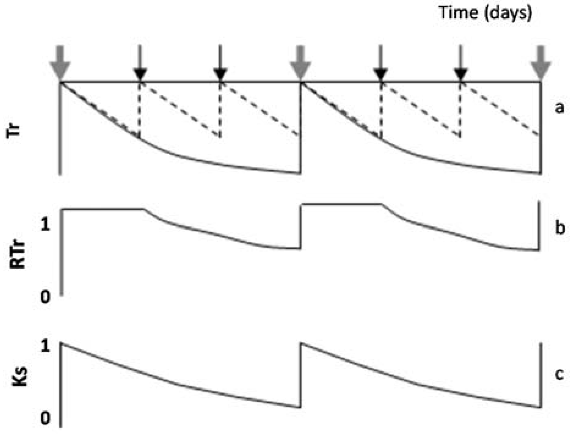
When intervals between irrigation are larger than one day, RTr or RET differ from Ks. This paragraph describes how this nuance, RTr or RET in relation to Ks, can be taken into account. Simulating a hypothetical seasonal course of daily Tr, in a plot considered well-irrigated and a stressed plot (diagram of
Figure 4a) during two cycles between successive irrigations in the stressed plot,
Figure 4b displays the resulting values of RTr for the stressed plot. A platform appears (RTr = 1) representing the period with simultaneous Tr decrease in both treatments. In that case, and to obtain Ks, the value of ET or Tr for the irrigated plot (here used as a reference to calculate RET or RTr) is conveniently replaced by another reference: ETo × Kc or ETo × Kcb. The value of Kc selected corresponds to the day after irrigation, and it is assumed as constant between two irrigation events (for simplification). By doing so (using ETo × Kc as reference), the platform (
Figure 4b) disappears, and Ks is obtained (
Figure 4c). In such cases, the initial platform is partly an artifact due to the simultaneous ET decrease in both treatments, during the first days in each stress cycle, until the irrigated treatment receives the second irrigation. If the weather is not stable, Kc can slightly increase when ETo decreases [
77], explaining some scattering in Ks values. The example later described for Peach Orchard 1 illustrates this process with experimental data.
Finally, it should be stressed that the relationships described by Denmead and Shaw [
49] between RTr and Ψ
s for different rates of ETc correspond approximately to the relationships between Ψ
p and RTr, considering Ψ
p as a surrogate of Ψ
s in the roots’ vicinity, at the moment measurements are taken. Ψ
p should have the advantage of less distance between the Denmead and Shaw [
49] lines for different ETc rates, which is likely due to less dependence on soil hydraulic conductivity for the relationship RTr-Ψ
p, in relation to the relationship RTr-Ψ
s.
8. Ks Functions: Case-Studies
Examples of case-studies where stress functions have been explicitly obtained and displayed are relatively rare for woody crops. To illustrate and discuss the variability found, a survey of several case-studies is briefly presented in this section. The experiments referenced here were carried out in different locations in Portugal, between 1994 and 2010, on woody crops and using the same approaches, thus making the results easily comparable. The aim is not only to compare results for a critical analysis, but also (as later described for Peach Orchard 1) to illustrate some steps that must be overcome to get such comparable results. The results presented here relate only to the stress functions obtained, other details and results being found in the work referred to for each case.
In all cases, eddy covariance data (ETEC) were used to calibrate the data obtained by SF techniques combined with weighted lysimeters data (Es). The difference ETEC − Es is called TrEC.
The EC system measured sensible heat flux density and latent heat flux density, the latter being converted to volumetric water flux density, or stand ET. In all cases, the energy balance was used in its simplest form (not considering advection or changes in energy stored at canopy level). The usual corrections for air density variation [
104] and UV radiation absorption by oxygen [
105] were performed. EC data were selected according to fetch and footprint analysis [
106] and validated through spectral analysis [
107], as well as through energy balance equation closure [
108]. There was no forcing to zero of the closure error, due to its small value and doubts about the correctness of this procedure. The sensors used were first (until 1997) a 1D sonic anemometer with a fine wire thermocouple and after 1998, a 3D sonic anemometer and a krypton hygrometer (respectively, Models CA27, 127 and CSAT3 and KH20 from, Campbell Scientific, Inc. Logan, UT, USA).
Tr
EC obtained as above was compared to uncorrected SF data for the periods with both measurements, as described in general in Ferreira et al. [
10,
109] The relationships obtained allowed the estimation of long-term Tr from SF data, generally obtained with the heat dissipation method described by Granier [
110], using sensors from UP GmbH (Cottbus, Germany) installed on representative plants. The probes (diameter 0.002 m, length 0.01 or 0.02 m) were inserted 0.1 m apart. SF was calculated assuming that all sectional area was effective (vines) or was estimated from destructive measurements with colorants, cores samples and radial flow profiles using the heat field deformation method (e.g., [
111]). Corrections for the influence of natural thermal gradients in the trunk were made. The upscaling technique was adapted to each situation, depending on the observed relationships between SF density and plants’ size, the heterogeneity in between and within measuring points (radial and azimuthal) and other considerations usually taken into account in such tasks. After calibration and corrections, these values were considered equal to Tr, on a daily basis.
Es, if any, was added to the corrected Tr, to obtain long-term ET. When Es was not negligible, it was measured with a set of 9 to 16 microlysimeters, having 15 cm internal diameter and 12 cm height, built and used as described in Daamen et al. [
112]. The soil cores were taken from a different place every day and the lysimeters reinstalled. Es was calculated by a weighted average in relation to the area represented by each lysimeter (with respect to distance from the emitter), and results were accumulated for daily values of Es. Details are described in the cited publications within the specific items below.
Water status was quantified using Ψp (surrogate of soil water status) measured in a variable number of healthy adult leaves (number depending on the scattering found, in order to obtain an average with an acceptable degree of confidence, on average 10 to 15 leaves) with a portable Dixon-Scholander type pressure chamber (Manofrígido, Lisbon, Portugal, 0.01 MPa resolution, pressure range 0 to 6 MPa, or a PMS 600, PMS Instrument Company, Albany, OR USA, 0.02-MPa resolution, pressure range 0 to 4 MPa, Dixon 1914). Data for θs are not used here, as some crops had deep root systems or stony soils making a representative value for θs or Ψs not measurable.
ETo was calculated according to Allen et al. [
29] using data from nearby standard meteorological stations and complemented when necessary by data from experimental plots, duly adapted.
The climate in all locations is temperate of the Mediterranean type, either Csa or Csa in transition to Csb (Köppen-Geiger classification [
16]), with dry and hot summer and mild rainy winter.
Stress cycles were established in all cases except for most of the rainfed vineyards, in order to analyze relationships between Tr reductions and other water stress variables. This consisted of leaving one sub-plot, located outside the reach (upcoming wind) of the EC sensors, under stress for a specific period, while a reference subplot was maintained in well-irrigated conditions. The values of RTr during stress cycles were obtained from the corrected Tr data, dividing Tr of the stressed plot by the correspondent value of the well-irrigated plot. Results were normalized using the last day with well-irrigated conditions in both plots, to account for possible reduced sampling, using a multiplicative factor during the full cycle. For daily irrigation, RTr was considered equal to Ks. For rainfed or non-daily irrigation in the reference well-irrigated plot, Ks was obtained by dividing Tr by ETo × Kcb. In the case of rainfed crops, the discrimination from Kcb and Ks was a previously necessary task, as explained in the correspondent publications referenced. The main aspects specific to each experimental situation and relevant for this analysis are described below in Measurements. The Ks functions obtained are presented (1 to 4) followed by a secondary comparative analysis and discussion.
8.1. Peach Orchard 1
Experimental site and crop parameters: The first study site was located at Águas de Moura (Sado Valley, 50 km SE Lisbon, latitude 38°24′, longitude 8°45′, elevation near 0), climate Csa. The orchard (3.4 ha) consisted of a 4-y-old
Prunus persica ‘Maybelle’ plantation with an average height of 3.1 m, planted in a sandy soil in a 5 × 2 grid. Sprinkler irrigation was applied at intervals of 3 to 4 days. Each sprinkler (one for two trees, i.e., for 20 m
2) irrigated (soil surface level) a circle of about 2 m
2. By the end of July, the leaf area index (LAI) of the canopy was 1.38 (
n = 15), and the ground cover (GC) was 60% ± 5% (
n = 32); other details about this experiment and its results can be found in Ferreira et al. [
78,
81].
Measurements: Xylem SF (m
3 s
−1) was measured on three trees from each plot (A and B) using a heat balance method that takes into account the variations in trunk heat storage [
113]. These values were considered equal to Tr, on a daily basis. Xylem sap flux density was also measured on five trees from each of the three plots using 2 cm-long continuously-heated probes, according to Granier [
110] and up-scaled. All sensors were connected to CR10, 21X and CR7 data-loggers (Campbell Sc. Ltd, Logan, UT, USA) recording 20-min averages. Lysimeters were used to measure Es and to obtain a locally adapted model. Plot A was kept well irrigated, while Plot B was subjected to water stress during successive periods of June (DOY 164 to 182) and July (DOY 189 to 205).
Ks functions: The relationship for relative transpiration (RTr = T Plot B/T Plot A) experimentally obtained using Ψ
p was: RTr = 1.28 exp (1.474 Ψ
p) with
r2 = 0.85 [
81]. Concerning RTr based on SWD, some steps are shown for a more detailed analysis.
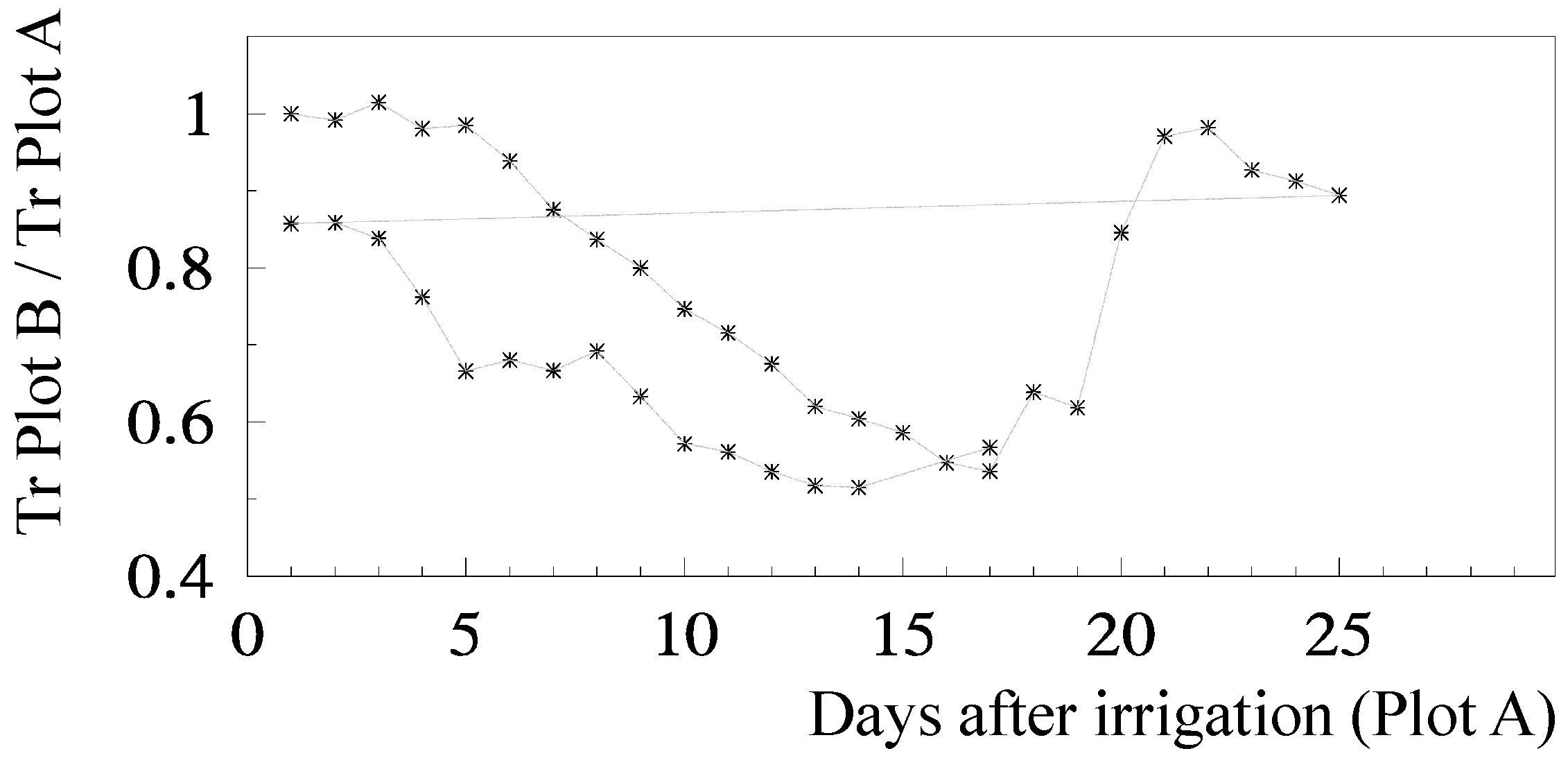
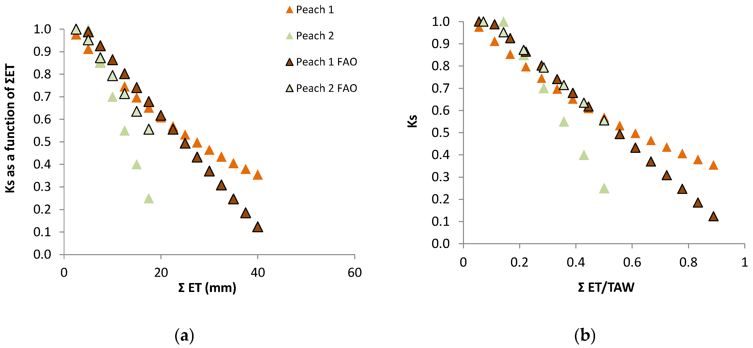
Figure 5 shows the temporal evolution of RTr, measured with SF methods on eight trees per plot, for the two cycles considered, as a function of the number of days after irrigation. After irrigation at the end of the first stress cycle, there is a period with RTr close to one, followed by a decrease before differences in irrigation between plots were again established, a typical behavior in orchards. The second cycle begins with RTr close to 0.9 probably due to the loss of leaves observed because of the previously imposed water stress. Consequently, the values of RTr for the second cycle were modified by a normalization, to be compared with the first cycle.
The relationship between RET (=ET Plot B/ET Plot A) and the sum of ET since the day after irrigation on Plot B (ΣET) is presented in
Figure 6a, for both cycles, after normalization of the second cycle and consideration of the Es component.
RET was calculated in relation to Plot A, where ET is also decreasing between two successive irrigations (when ΣET < 8 mm and RET = 1, ET is simultaneously decreasing in both plots,
Figure 6a). As a consequence of this, the ET does not seem to be reduced until the value of ΣET = 8 mm. This artifact was eliminated by the consideration of the ET reduction in Plot A, using a climatic reference (
Figure 6b). The equation better adapted to the range of points shown was Ks = 1.044 exp (−0.027 ΣETa). ΣETa is later (
Section 9.2) divided by an approximate value of AW = 45 mm. The relationship between Ks and Ψ
p is displayed later (
Section 9.1) as RTr = 1.28 exp (1.474 × Ψ
p).
8.2. Peach Orchard 2
Experimental site and crop parameters: The experiment took place during the summers of 1998 and 1999, in a 60-ha orchard near Montijo, Portugal (38°42′ N, 8°48′ W, elevation near zero) where, as before, annual rainfall was around 600 mm and mean air temperature around 16 °C, climate Csa. The orchard consisted of
Prunus persica [L.] Batsch ‘Silver King’ trees planted in 1996, at 5 × 2 m spacing, on a sandy soil (an Arenosol, according to the FAO classification). The trees were drip irrigated (2000 emitters/ha with a flow rate of water of about 3.5 L/h per emitter). The tallest branches reached 3 to 3.5 m. GC was 29% (shadowed areas near solar noon), and LAI was 1.2 (1998) and 1.4 (1999). Other details about this experiment and its results can be found in Paço et al. [
80,
114,
115].
Measurements: SF was measured from June to September using six sensors each year in the irrigated plot, with a 1-cm (1998) or a 2-cm length (1999). Corrections were explicitly made for the influence of natural temperature gradients in the trunk and also took into account the radial profile of SF distribution. Es was measured with five microlysimeters in the row and four between rows, near the limit of the vertical projection of the canopy. Long-term Es was obtained with specifically developed models, as a function of ETo and the available energy at the soil surface, as detailed in Conceição et al. [
116]
Ks functions: In this case, the equation better adapted to the range of points for the stress cycle was a straight line: Ks = −0.06 ΣETa + 1.30, valid for the range 0 to 20 mm (
Figure 3). Using Ψ
p, Ks obtained experimentally = 1.60 exp (2.54 Ψ
p), in the range −0.2 to −0.9 with
r2 = 0.92 [
80]. The differences between the two lines for similar peach orchards are discussed in
Section 9.
8.3. Vineyards
ET and Tr data from five experimental vineyards were described in Ferreira et al. [
20]; here, only four vineyards suffering considerable stress were used for the discussion of Ks functions. In general, the maximal measured values of Kcb (when Ks = 1, in late spring or early summer) varied from 0.75 to 0.35, depending on LAI (
r2 = 0.90) or GC (
r2 = 0.81), related as LAI = 0.054 GC + 0.378 (
r2 = 0.76). The main features of the selected vineyards and Ks functions are described in the following; for a more complete description of sites and methods, see Ferreira et al. [
20] and the references specific to each experimental study.
8.3.1. Vineyard Experimental Sites and Crop Parameters
Vineyard 1 (V1): Tagus Valley (Portugal), 39°10′ N, 8°43′ W, 5 m above sea level, a.s.l., area: 24 ha, fetch 600 m, climate Csa.
Vitis vinifera ‘Trincadeira’, grafted on SO4, planted in 1984, density: 3030 vines per ha (3.0 m × 1.1 m), rainfed. Soil: deep clay sandy loam. LAI at veraison 2.39 and 1.96, for 1996 and 1997, GC (shadowed areas near solar noon): 28%. A detailed description can be found in Silvestre and Ferreira [
117].
Vineyard 2 (V2): Alenquer (Portugal), 39°04′ N, 9°06′ W, 155 m a.s.l.
Vitis vinifera ‘Castelão’, grafted on 1103P, planted in 1993, density: 3333 vines per ha, rainfed. Soil: Loam. LAI at veraison 1.66, GC: 16%. Climate: transition Csa/Csb (detailed description in Ferreira et al. [
109]).
Vineyard 3 (V3): Palmela (Portugal) 38°35′ N, 8°49′ W, 25 m a.s.l. 216 ha, fetch > 1000 m.
Vitis vinifera ‘Syrah’ grafted on 1103P, planted in 1990, density: 2975 vines per ha (2.8 m × 1.2 m), rainfed. Soil: deep clay sandy (ARh) FAO classification. LAI at veraison 1.32, for 2002, GC: 18% (detailed description in Silvestre [
118]).
Vineyard 4 (V4): Beja (Portugal), warmest and driest region of Portugal (Alentejo), 38°03′ N, 7°55′ W, 200 m a.s.l.
Vitis vinifera Aragonez ‘syn. Tempranillo’, grafted on ‘1103P’, planted in a grid of 2.8 m × 1.1 m area in 6 ha surrounded by a continuous area of a 30-ha vineyard. Soil: shallow clay Vertisol with abundant gravels and few stones, derived from basic rocks. Main root zone depth is about 0.6 m; some fine roots explored rock fissures up to a 1.5-m depth. LAI at veraison 2.15, GC: 42%. The vineyard was drip irrigated, with emitters every 1.0 m (flow 2.4 L/h), suspended above the ground in the vine row (detailed description in Ferreira et al. and Silvestre et al. [
20,
103]).
8.3.2. Measurements
A strong relationship was observed from the first experiments, between vine leaf area and SF for individual plants, thanks to low SF azimuthal variability within a plant. Therefore, upscaling was performed using the following five step procedure: (1) measurement of SF of individual vines; (2) determination of leaf area of those vines; (3) calculation of average SF on a leaf area basis; (4) determination of stand LAI; and (5) multiplication of stand LAI by the SF per unit of leaf area obtained in Step 3. Except in the case of Plot 4, during 2010, there was not a plot irrigated for reference (ETc), ETc being obtained either for the periods without water stress or following local application of water to FC in one subsample of plants with SF sensors.
8.3.3. Ks Functions Observed in Vineyards
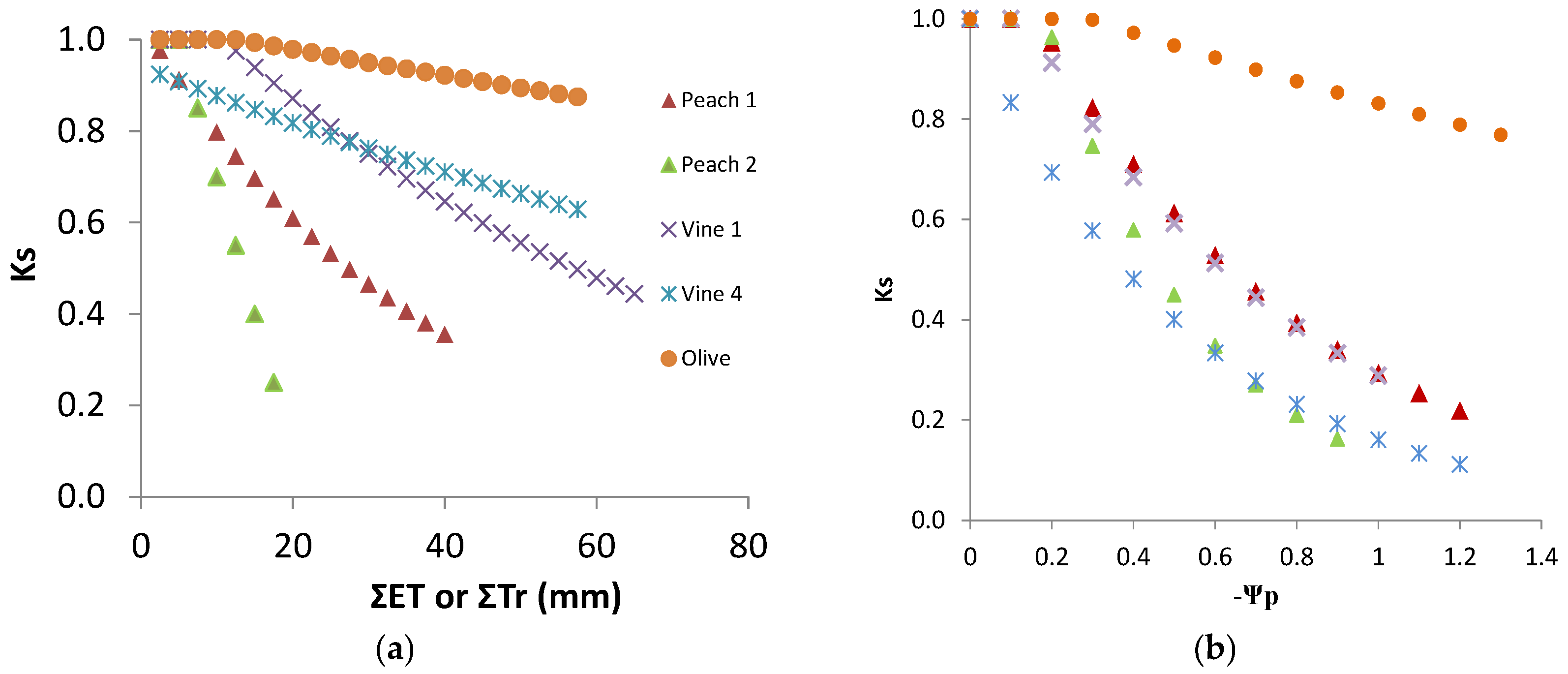
The discrimination between Kcb or Kc and Ks coefficients provided Ks, which, in these water stressed conditions, was obtained as Tr/ETo divided by Kcb. Ks decreased from one to 0.2 (irrigated vineyard in dry area), and in several rainfed vineyards, it remained above 0.5 by the end of summer [
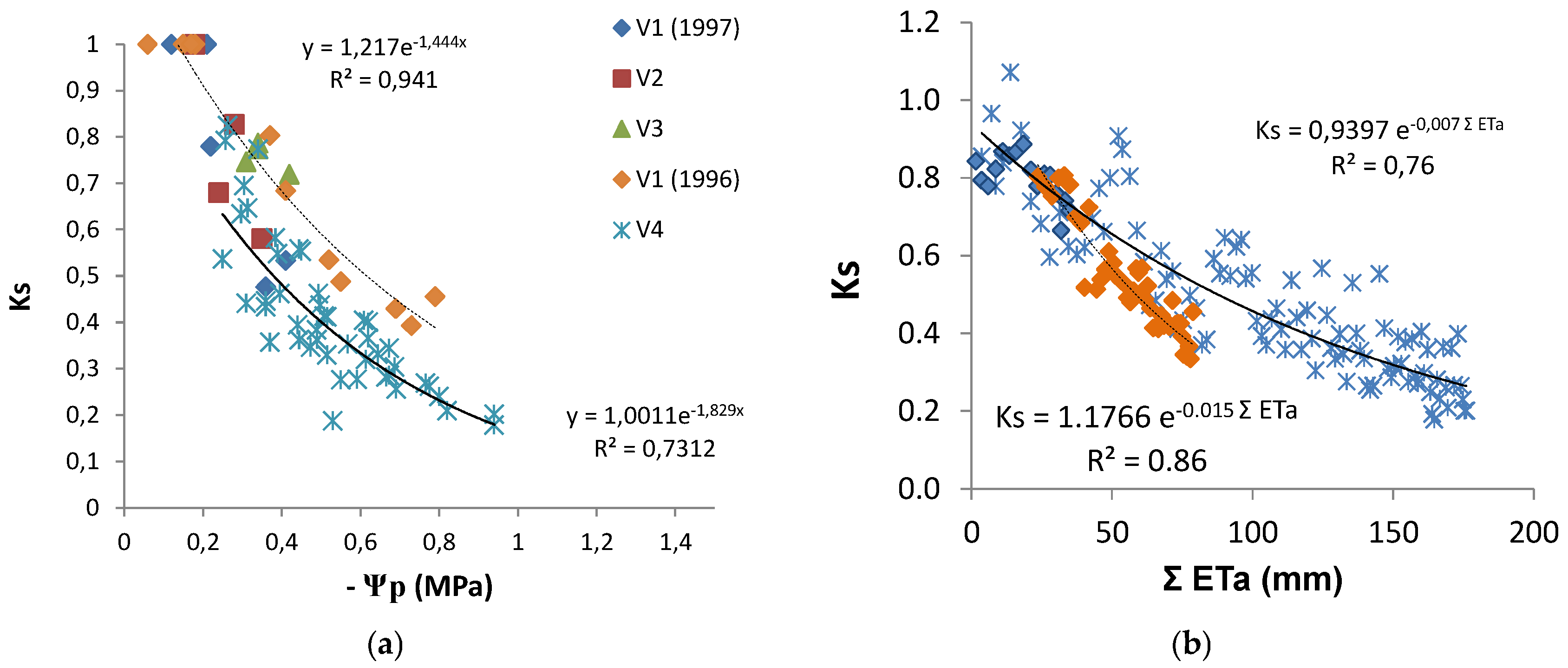
20]. Such low Ks values are experimental evidence of the relevance of considering Ks when estimating Tr. The relationship between the increasing absolute values of Ψ
p and the Ks values observed (
Figure 7a) shows a similar concave line (decreasing slope as stress progresses), with the slope of the trend line for each individual vineyard, higher for the higher values of maximal crop Tr (soil near FC). There is a large apparent scattering (25 to 30% variation around average). With the exception of two points for V2, the line corresponding to the situation where and when Ks is higher for the same Ψ
p refers to the location and year with lower atmospheric demand (DOY 200 to 252, 4 mm/day), while the lower line shown corresponds to the location with higher atmospheric demand (DOY 200 to 252, 6 mm/day) when sub-plots with DI were considered (2010). The relationship between Ks and ΣETa (≈ΣTr), for the periods when Tr data allowed the calculation of measured ΣTr, is shown (
Figure 7b) for the vineyards corresponding to the two lines of
Figure 7a.
8.4. Olive Trees
Experimental site and crop parameters: The study site was located in the Alentejo region (Portugal), 30 km from Beja (38°1.34′ N, 8°10.84′ W, 97 m a.s.l.), annual rainfall 572 mm (1971 to 2000, IPMA, 201). The orchard (10 ha in a farm of 434 ha) consisted of 7-y-old trees (
Olea europaea ‘Arbequina’) planted over ridges in 2004, in a sandy-loam Luvisol in a grid of 4.8 m × 7.0 m. Irrigation was made by drippers in the tree row spaced 0.75 m. LAI and GC ranged between 2010 and 2012, from 1.0 to 1.3 and 17 to 18%. Other details can be found in Häusler et al. [
119]
.Measurements: Specific items were, in order to account for the natural gradients, a third probe was added to each commercial SF sensor (two probes, UP GmbH, Cottbus, Germany) installed in seven representative trees in the main plot. A stress cycle was induced during six weeks in 2011 (DOY 215 to 258). During the stress cycle presented here, another six trees in each sub-plot were equipped with SF sensors in two small subplots (Plot 2 and Plot 3: 941 m
2 and 28 trees each) with independent irrigation systems. As before, the SF data were related directly with values considered reliable at the stand level (ET
EC-Es), with Es from a specific model to get the seasonal time course of Es for summer time built from microlysimeters data [
120]. The relationship obtained was used for adapted upscaling of SF data to the stand level Tr [
121].
Ks function: One stress cycle was used to relate water stress indicators and allowed the determination of a stress function relating the increasing absolute values of Ψ
p and correspondent Ks values, as Ks = 1.079 exp (0.261 Ψ
p) with
r2 =0.90 (range Ψ
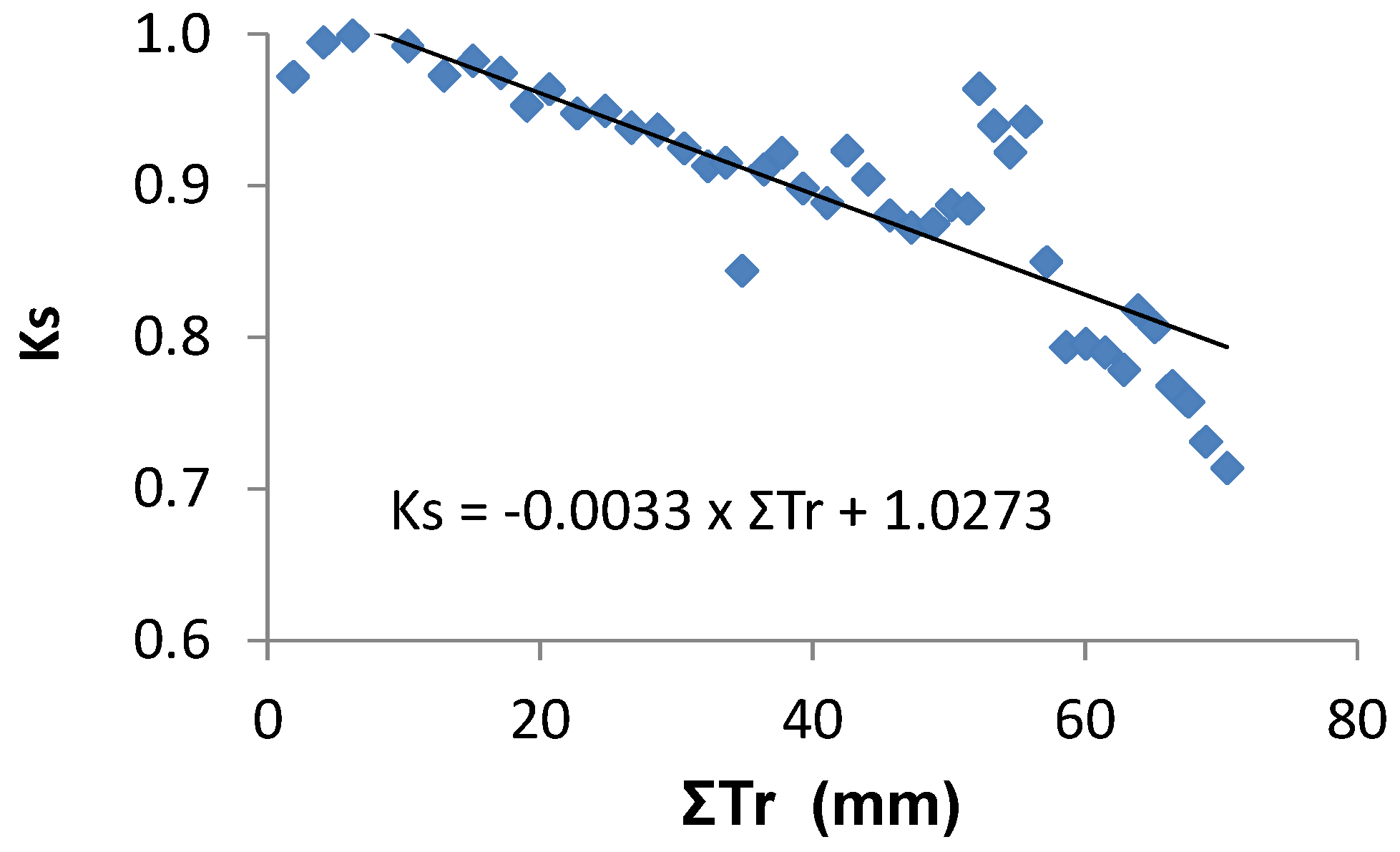
p −0.1 till −1.3 MPa). Using the cumulated Tr (since last irrigation) in the sub-plot submitted to stress, a linear function Ks = −0.003 ΣTr + 1.0273 was obtained (
Figure 8). The scattering in the relationship with ΣTr was due to the occurrence of cloudy days during the stress cycle with some precipitation (7 mm).
9. Discussion on Presented Ks Functions
9.1. Comparing Experimental Ks Functions
The experimental equations above were established either with SWD expressed in mm (
Figure 9a) or with Ψ
p (
Figure 9b) where the equations correspond to the statistical adjustments to the experimental observations, described above, applied for Ks ≥ 1. SWD was represented by either (i) ET accumulated (ΣET) since the last time the soil was at FC or (ii) in Vineyard 4, ΣET accumulated since the experimentally measured Ks started to decrease. Very distinct lines were obtained for the five situations considered in
Figure 9a. The consequence of using the procedure (ii) for V4 was that the platform corresponding to RAW almost disappears from the graphical representation (apparent
p very low). This artifact was justified by the need to better represent and compare the lines (slopes), which would otherwise be much farther apart (
Figure 9a).
In general, the slope was much higher for plants having smaller root systems, especially the daily drip irrigated peach orchard, while those having access to water in deep soil, and the other species, eventually more adaptable to rainfed conditions, were in the other extreme.
It is expected that the lines representing these functions would merge by considering SWD (mm) in relation to TAW, i.e., expressed as a percentage. For this to be possible, it was necessary to have reliable values of TAW. This value is very difficult to obtain when the soil volume explored by sparse roots has to be quantified. TAW was roughly estimated as 45 and 35 mm for Peach Orchards 1 and 2, respectively, with uncertainties due to anisotropy. When using SWD expressed as a percentage (ΣET/TAW) for the deeper root systems, the result obtained was deceptive as only for apparently unrealistic values of TAW would all of the lines clearly be close to each other. This observation implies a key difficulty in using this operational approach, whenever plants have deep and sparse root systems. The fact that one or the other variable is preferred (ΣET or Ψp) is therefore also related to the extension of the root system, the latter offering a more attractive option for plants with deep roots, but requiring measures of Ψp.
Concerning the Ks functions based on Ψ
p, the case-studies described were also used in a comparative analysis (
Figure 9b). All equations were exponential of the form Ks = a exp (b Ψ
p). The use of a non-linear fitting is consistent with the non-linearity of the hydraulic conductivity as the soil dries out, with a decreasing slope expected.
For the woody stands with larger root systems, the relationship with Ψ
p again provided very distinct response curves. The difference was so sharp that the variances discussed in
Figure 7a for vineyards become comparatively less dramatic. As discussed in Ferreira et al. [
20], the separation between lines (mainly V1 to V4) suggested that the distinct levels of the atmospheric driving force contributed to the explanation of the different trends, due to its well-known influence on the shape and slope of Ks functions. Conversely, the scattering around each line (experimental data) could be explained by the artifact of Kcb changing steadily from day to day or being constant in a short interval, while it has been shown that it changes on a short time scale (inter-daily), increasing when the value of ETo decreases (e.g., as shown for kiwi [
77]).
All of these differences call for the need to use modelling with not only an appropriate water stress indicator, but also parameters adapted for each particular case.
Again, the relationships obtained (
Figure 9b) displayed a gradually decreasing slope as root systems were larger: vines and olive trees seemed to be much more resilient to water shortages, with much lower slopes of the Ks function, but with clear differences between them.
Even if these statistically adjusted lines do not match the experimental points perfectly, we can confirm (
Figure 9) the aspect observed in
Figure 7: for the same value of Ks, V1 (1996) showed a lower potential (Ψ
p) than V4, for a lower value of ΣET. This means that, in this soil, these plants (V4) were able to extract more water or withstand significantly lower values of SWD with a lower reduction in its water status. In other words, for the same Ψ
p, V4 had a notably lower Ks, corresponding to a higher value of ΣET in relation to V1. V1, rainfed, was in more favorable soil and climatic conditions (V1, loamy soil, deep and access to the water table, while V4, stony, poor soil, no water table). V4, in spite of being irrigated, seemed to have a more conservative behavior as, for longer periods, it acquired significantly more water in total, at very low rates. These results were consistent with Tron et al.’s [
122] findings, in that plants characterized by a cooperative root system seemed to be less prone to water stress while plants with non-interacting roots appeared to better thrive in climates with less probability of drought. By cooperative root systems, those researchers included the possibility of hydraulic redistribution in the root systems (as described in [
123] for olive).
9.2. Comparing Experimental Data with FAO Ks Simple Model
The Ks functions obtained experimentally for Ks versus ΣET were compared with simulated results, using the very simple model equation (Equation (2)) proposed in [
29]. For peach orchards, the depletion factor values (
p) considered were the ones obtained experimentally (close to 0.1). Provided the values for
p are the ones obtained in situ, which are very different from the ones recommended for average conditions (e.g., [
29]), there was a good agreement between experimental evidence and the model (
Figure 10a,b). An overestimation for Peach Orchard 2, as well as an underestimation for Peach Orchard 1 in the lower range, was noticed. If the usual
p values recommended were applied to these two situations, the models would perform in a very unrealistic way. The main shortcoming in these conditions (sandy soils, high ETo rates, plants relatively sensitive to stress) seemed to be the reason for the lack of performance of
p estimations.
This FAO model (Equation (2)) was also applied to the stands with deeper roots. However, in such situations, good predictions were only possible for values of TAW that would not result from any apparently reasonable application of the usual procedure, if considering only the apparent geometry of the root system and the soil parameters.
Again, comparing the two lines for peach orchards, the difference (
Figure 9a and
Figure 10) was sharp despite all conditions being similar except for irrigation. This difference was attributed to the fact that with mini-sprinkler irrigation every 3 to 4 days (Peach Orchard 1, plants were used to moderate stress between irrigations) and had much larger root volume than daily drip irrigation (Peach Orchard 2) and consequently a better resilience to imposed water stress. This was consistent with expectations from theory, concerning the analysis of limitations to water movement in soil due to low hydraulic conductivity and high density roots in a small volume, as discussed above and in Paço et al. [
80]. A poorer adaptation to water stress for the drip irrigated orchard (higher density and smaller volume of roots) apparently promoted a sharper decrease. Eventually, these drip irrigated trees submitted to such stress levels (short stress cycle) did not have enough time to make the required physiological adjustments to water scarcity that to some extent usually occur over a longer term.
For Peach Orchard 2, at 50% of TAW consumption (ΣET/TAW = 0.5), the Ks error by the FAO model (
Figure 10b) was higher than 100%, with similar error in Tr estimates.
In conclusion, concerning the use of the FAO Ks model (Equation (2)) versus experimental functions, for plants with not too large root systems, when TAW can be estimated with some confidence, the model seemed to be a good tool within the range of stress usually noted for DI, with the condition of the adjustment of
p to observed values or good estimates. When considering the x axis expressed as a percentage of AW used (SWD in percentage), the scattering was reduced for the upper range of Ks values (
Figure 9b). This approach seemed to accommodate the impacts of different soils well for the situations described, but the influence of very distinct root patterns and densities was more difficult to account for, as shown by the differences in the two lines for peach orchards. The lack of applicability of these models to olive orchards and vineyards seemed to also be related to root architecture, due to the inability to quantify with reasonable precision the soil volume explored, in such a pedoclimatic context. Therefore, it was not possible to make a sound comparison concerning the reliability of the model in situations of deep sparse rooting, as seen in olive orchard and vineyards.
9.3. The Practical Use of Ks Functions
The Ks-ΣET relationships provided an answer to the questions of when and how much and can be auto-sufficient if well-adjusted, as there is no need for in situ measurements, as exemplified in Ferreira and Valancogne [
89] and Ferreira et al. [
19]. They are used in many algorithms for irrigation scheduling. It is enough to select a critical threshold value for Ks or for SWD (either in mm or percentage).
The relationship Ks-Ψ
p can also be directly used in irrigation scheduling, if Ψ
p is measured and a specific threshold value for any of these variables is selected: (a) from Ψ
p data, the Ks function can be used to estimate ETc × Kc × Ks, the SWD and consequently the irrigation depth, once a threshold value for Ψ
p is predefined; or (b) if a threshold Ks value is predefined, the user can decide when the right moment to irrigate arrives, from measured Ψ
p data by using this Ks function. Irrigation should take place when the measured value of Ψ
p corresponds (from the equation) to the selected Ks threshold. In anisohydric plants/conditions, Ψ
stem can be used instead of the values at predawn [
124].
In homogeneous low crops, the soil water status follow-up has enough precision for scheduling irrigation, with advantages. In fact, soil water status is the only water status indicator that serves both as a prompt when to irrigate (once a threshold selected) and also how much to irrigate, as its follow-up reveals the SWD to determine irrigation depths. Whenever soil water status cannot be directly quantified or when the possibility of getting representative values is limited by the associated cost, the two variables above (SWD or ΣET and Ψp) are an alternative for representing soil water status.
Other water stress indicators are not considered in the quantitative approaches discussed, for several reasons: thresholds are not stable/robust (e.g., diameter variations), or do not apply to all plants (e.g., Ψ
stem), or are too time/resource consuming (e.g., measuring g
c), or data are too expensive, or, thus far, are not often available in real time or with enough precision (e.g., remote sensing [
125]).
If locally valid Ks functions based on those (ΣET or Ψp) or other variables are not available, Equation (2) can be used with uncertainties and precautions that require a complementary approach.
10. Uncertainties and Combined Approaches for Irrigation Scheduling
There are many sources of uncertainty, not only in quantifying Ks, but also in other steps of ET estimation to schedule irrigation. The easiest situation is when soil measurements can be performed for occasional checks, in order to verify the adequacy of Ks function and all of the associated procedures to get ET. If the estimated value for SWD is significantly different from the measured value, the process can be adjusted by developing a self-learning routine, which can be automatic or not. The users or those who work on such algorithms need to discriminate the main causes of estimation errors and their specific consequences. Those errors can occur either in the estimation of ETa, or other components of the water balance (1 to 10), or in the soil measurements used for regular or occasional checks (11 to 12), as described in the examples below.
errors in ETo estimation due to inadequate data, (a) for instance, lack of quality control of meteorological data or (b) in the selection or application of equation to estimate it or (c) errors (e.g., units, time scale);
inadequate values of ETo estimated at the precise location of the study, due to microclimatic differences between that location and the one where the data are collected, as well as any other adaptations required due to slope, aspect, row orientation, wind channels, buildings or other very local sources of positive or negative advection;
inadequate Kc values used due to unsuitable values (tables) or equations to estimate it;
inadequate Kc values used due to incorrect evaluation of parameters or variables used for the estimation process (plants high, LAI, ground cover, wet fraction, etc.);
inadequate Ks function used (p, slope, shape);
errors in precipitation data or unsuitable values due to local effects;
errors in estimating irrigation depths (plus volumes applied);
ignored effects of other sources of water than those usually considered (soil water storage capacity, irrigation and precipitation), such as fog interception, dew, capillarity rise, hydraulic lift and access to the water table;
errors in quantifying irrigation efficiency, either due to ignored losses from runoff or deep percolation to the water table, erroneous estimations of it, or errors due to any other approach related to quantifying such sinks;
lack of representativeness of soil water content values, due to insufficient sampling or location;
errors in soil water status measurements, due to faulty functioning of the sensors or incorrect calibration;
errors in root volume, FC and PWP values, for estimating soil water balance and soil water storage capacity (contribution from soil in early season) and to convert θs to the actual level of AW, for the interpretation of the measurements and the use of selected thresholds, and so forth.
The following actions are examples of suggestions to solve some correspondent problems identified above, such as:
- (a)
errors in ETo: look for qualified support in selection and application, for adapted equations, for good quality data obtained in standardized reference conditions and correct equation use;
- (b)
in relation to (2) and (6), use simple evaporimeters or udometers to compare locations, in relative terms (microclimate, local advection, buildings, shelters, etc.);
- (c)
once this is solved, check possible errors in Kc (3 to 4): look for qualified support and good parameter evaluation at the plot level; for out-of-control, inappropriate subroutines for Kc, use a self-learning feed-back, such as verifying if the error is systematic and cumulative along the vegetative cycle and if it occurs even without stress (increase or decrease), and in the positive case, adjust Kc by trial and error;
- (d)
errors in Ks function (5): verify if the error only appears when stress periods start; test the parameters as p (to obtain the RAW) or the volume in mm, independently of RAW estimations; use reliable and daily ETc observations to build site-specific function;
- (e)
more specific measurements to solve (7) (8) (9) and (12);
- (f)
soil measurements: increase sampling; check for better sensor location; use more reliable methods; check for proper interpretation of outputs, in relation to the so-called calibration process; occasionally analyze outcomes from soil sensors not representative versus plant water status and modelling, to understand the relative value of them; and adjust the interpretation of their outputs.
The general assumption is that it is possible to evaluate the correctness of the estimation process by comparing available and appropriate soil water status measurements with estimations by means of a soil water balance. Trying to distinguish between sources of error is crucial. This approach goes beyond a simple feedback approach, or just adjusting irrigation depth to maintain the water status in a certain range. This approach actually aims at first using a feed-forward approach [
74] assuming it has many sources of error and therefore learning from the feedback process, in order to adjust the estimation algorithm, accumulating knowledge for future use. Ideally, in a very successful process, the user would become almost independent from soil water status follow-up. This is apparently more straightforward, when using soil water status, especially θ
s, but can be adapted to the use of any other water stress indicator. All of this process is a combination of using SWD estimations (ET modelling) with follow-up using water stress indicators, continuously or not (occasional checks).
Another situation when this combination could be fruitful concerns the use of a percentage of ETc to schedule DI. It can be argued that this approach to applying DI leads to temporary uncertainty in obtaining the level of water stress desired (
Figure 11). Furthermore, often the so-called full irrigation treatment is over- or under-irrigated due to poor experimental set-up or implementation. For instance, incorrect values of Kc (or Kcb) or lack of discrimination between Kc and Ks can misrepresent the outcomes from a DI experiment. For better precision in quantifying the stress levels applied in DI, adequate Ks functions, where Ks is related with any available water status indicator measured or estimated, could be used. This would enable an understanding of the situations and better transfer knowledge to the advantage of any other user. However, getting practical and reliable models to obtain Ks, for the Mediterranean woody crops that are our concern, is still a challenge for the future research in irrigation science.
11. Concluding Remarks
Stress functions (functions to get stress coefficients) are an important step for evapotranspiration estimates in the case of woody crops, especially in a Mediterranean climate due to deep root systems associated with edapho-climatic conditions. This is particularly relevant in scheduling deficit irrigation.
Stress functions are part of huge modelling packages for crop water requirements. These simple functions set limits to the capabilities of these models. It is important to be aware of those limitations, by analyzing the adequacy of several major individual steps of the calculation procedure.
Experimental stress functions were evaluated. The differences found in such functions, between the most well-known model (Ks function in FAO 56) and the experimental data, call for the need to use modelling with not only an appropriate water stress indicator as input, but also parameters adapted for each particular case.
Due to difficulties in modelling ET in woody crops and the increasing importance of deficit irrigation, there was an increase in the direct use of water stress indicators. Often, this approach is described as an alternative for scheduling irrigation. This is not entirely true because (1) for planning of irrigation projects, ET needs quantified and (2) for irrigation scheduling, the use of individual water stress indicators is just a feedback approach; it relies on trial and error and does not allow identifying the sensitive compartments/processes for improving capacities.
Only the combination of both (modelling ET and using water stress indicators directly) offers an opportunity to learn and transfer knowledge to other plots, crops and farmers. In addition, it offers the possibility to develop stepwise independent of measurements. Consequently, both feed-forward and feedback approaches should be combined to improve ETa estimations, as an investment for much broader applications in relation to the ones provided by single water status follow-up.
Water users in agriculture and landscaping will have to justify the amounts of water claimed. This will require physically-sound tools. The approach discussed offers suggestions to fulfill this requirement.
ET modelling in combination with measurements of water status also potentially contribute to the evaluation of the dynamics of natural stands, especially in relation to climate and land use changes. As stressed by Bodner et al. [
126], when discussing water conservation measures in complex root-soil interactions, understanding site-specific stress hydrology is required for efficient stress mitigation measures.


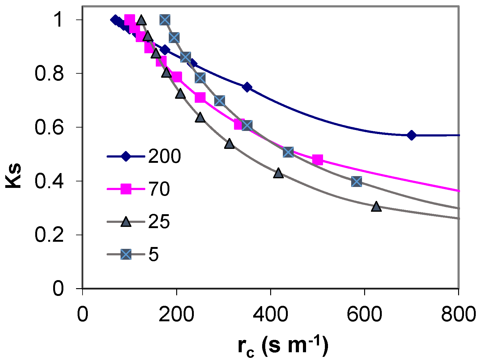
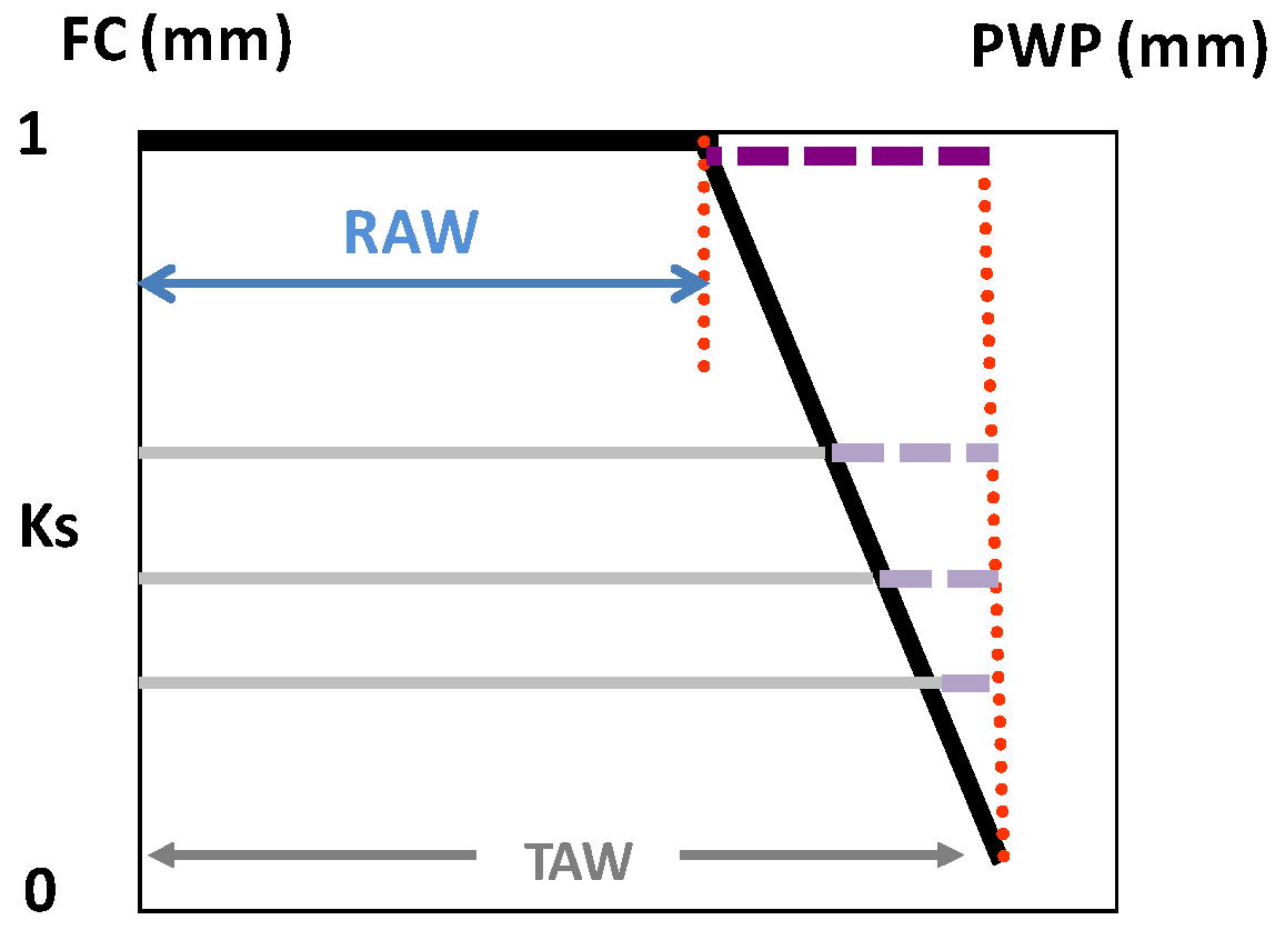
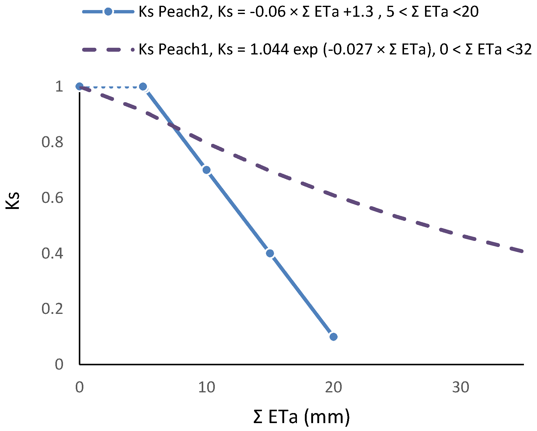
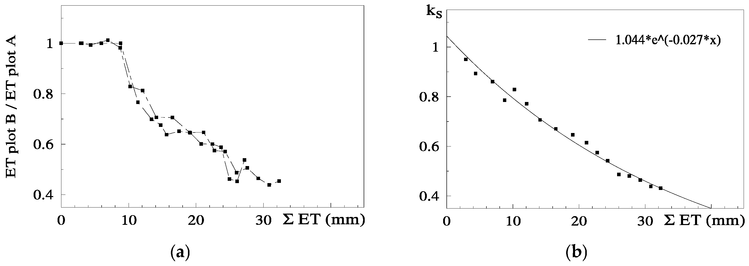
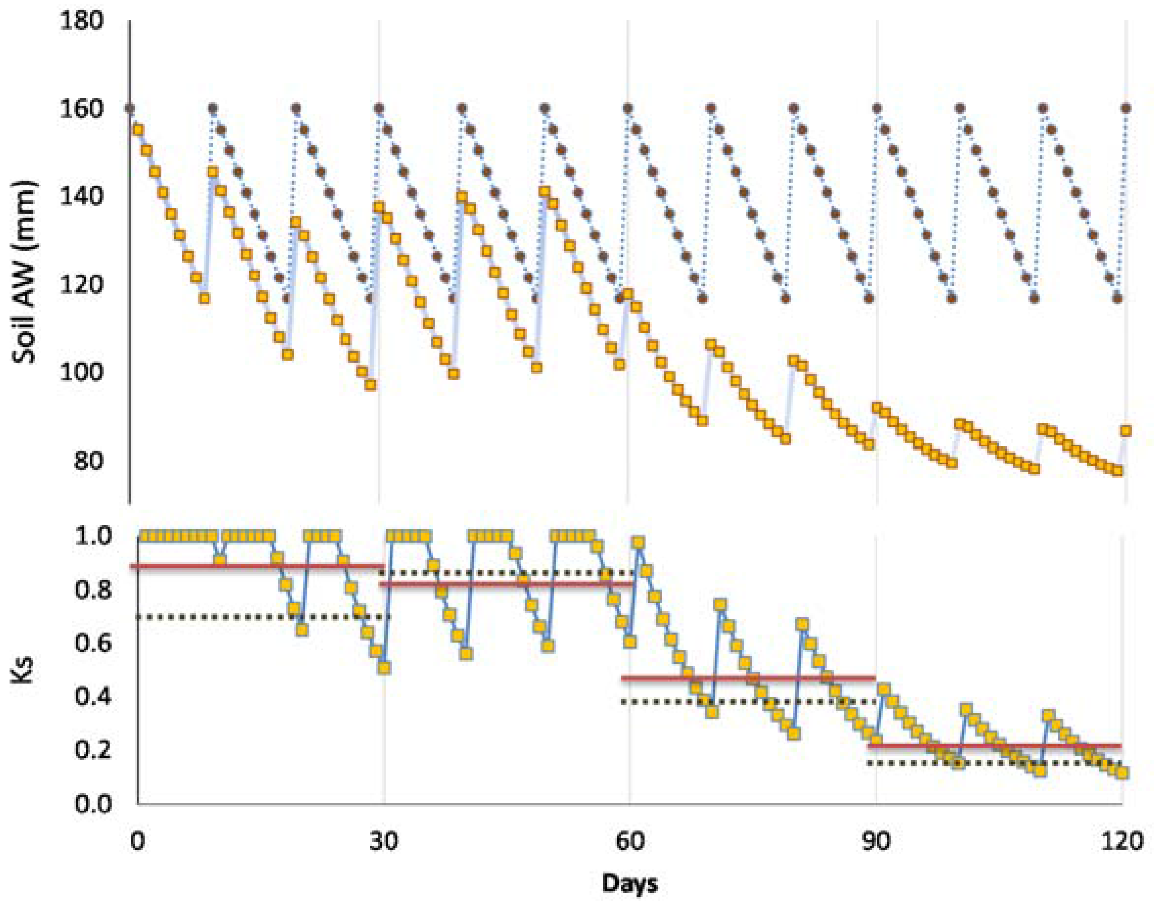