Article

Managing Water Stress in Olive (Olea europaea L.) Orchards Using Reference Equations for Midday Stem Water Potential

by
Marta Sánchez-Piñero
,
Mireia Corell
,
Alfonso Moriana
*,
Pedro Castro-Valdecantos
and
María-José Martin-Palomo
Dpto de Agronomía, ETSIA, University of Seville, Crta de Utrera Km 1, 41013 Seville, Spain
*
Author to whom correspondence should be addressed.
Horticulturae 2023, 9(5), 563; https://doi.org/10.3390/horticulturae9050563
Submission received: 11 April 2023 / Revised: 1 May 2023 / Accepted: 6 May 2023 / Published: 9 May 2023

Abstract

:
The irrigation surface of olive orchards has increased over recent decades. In zones affected, deficit irrigation scheduling is a must. The aim of this work was to study water stress management based on reference equations for midday stem water potential. An experiment was conducted over three seasons in Seville (Spain) from 2020 to 2022. A young hedgerow olive orchard (cv Manzanilla de Sevilla) was irrigated using three different treatments: Control (full irrigated), RDI, and Rainfed, in a completely randomized design (six replications). The midday stem water potential and leaf conductance were measured throughout the three seasons. Stem water potential was more sensitive to water stress than leaf conductance and showed a clearer impact and rehydration. Individual data of stem water potential were grouped according to leaf conductance reduction. The relationship of these stem water potentials and temperature or vapor pressure deficit was significant, linear, and aligned to published baselines. Scattering in these equations increased when the leaf conductance reduction was greater. These reference equations would be useful to define moderate water stress conditions in the most sensitive processes, such as vegetative or fruit growth. Definition of severe water stress conditions would be better established with constant values.

1. Introduction

Olive trees (Olea europaea L) are a type of Mediterranean fruit tree commonly cultivated in rainfed conditions. However, since the 1990s in the 20th century, the irrigated surface of this crop has been increasing. For example, in Spain, the first world producers, irrigated olive surface changed from almost zero in 1982 to more than 400.000 ha in 2021 [1]. The water available for irrigation of this fruit tree was commonly low because it is considered a very drought-resistant species, and the zones where they were cultivated had severe water restrictions. Therefore, deficit irrigation is a common practice in commercial olive orchards. In crops, the effect of drought on yield was related to the phenological phase, the level, and the duration of the water stress [2]. Regulated deficit irrigation (RDI) scheduling was based on this assumption [3], but while phenological phases that apply irrigation have been described for most fruit trees (i.e., [4]), there is less information on water stress management and the definition of level and duration.
For olive trees, as for other fruit crops, deficit irrigation scheduling was commonly defined using the percentage of crop evapotranspiration (ETc) (i.e., [5,6]). However, in some works, different plant water status indicators were also used to determine deficit irrigation scheduling for olive orchards (water potential, [7]; dendrometer, [8]). The main difficulty for these plant indicators would be to obtain a reference because they are strongly affected by environmental conditions [2]. Some authors [9] suggested a baseline equation for midday stem water potential in prunes to define “wet soil conditions”. This baseline was the relationship between stem water potential and vapor pressure deficit (VPD) under no water stress conditions. This approach has been used for other plant water status indicators. For maximum daily shrinkage (MDS), these reference equations were used to define the level of water stress as the MDS signal, firstly for almond trees [10] but also for other fruit trees [11]. For olive trees, different baselines have been reported using the midday stem water potential vs. maximum daily temperature [12] and VPD [12,13]. However, absolute threshold values had also been suggested for full irrigated conditions and water stress management [8,12,14,15,16]. Because the baseline would be considered the “wet soil conditions” [9], irrigation management that maintains water status in these values could negatively affect trees, for example with waterlogging problems. Moreover, some works [13] proposed that the baseline was not the target value for the midday stem water potential and the threshold had to be defined according to distance to this baseline. This water status being below the baseline would secure no “wet soil conditions” and would be near to an optimum irrigation. However, this approach assumed that the relationship between the midday stem water potential vs. evaporative demand would be parallel to the baseline when water stress increased, even in moderate water deficits conditions.
These reference equations could be defined according to the impact on leaf conductance. Water status measurements would characterize the soil–plant–air system, which would change with environment and water stress. The response of each indicator could be different and affect the values of other indicators [17]. Olive trees are considered very resistant to drought conditions. An estimation of 50% of loss hydraulic conductivity was obtained around −5 MPa of the xylem water potential [18], and significant gas exchange has been reported in conditions of very severe water stress [5,19]. Daily patterns of leaf conductance in olive trees were related with evaporative demand in fully irrigated conditions [20]. Such a response is uncommon in fruit trees and was considered as part of the response for the great resistant to water stress [20]. Water potential has been reported as an earlier indicator of water stress than gas exchange [21] in some works but not in others [22,23]. Some authors reported changes in the relationship between leaf conductance and evaporative demand as a function of the level of water potential [24]. Therefore, reference equations of water potential could consider the effect on leaf gas exchange to include more complete information about water stress management. In olive trees, the relationship between leaf conductance vs. water potential had been reported as two linear phases [15]. In the first part, a strong decrease in leaf conductance was found in a narrow range of water potential, while in the second phase, low variations of leaf conductance were associated to a great decrease in water potential. Some authors [25] suggested that these changing patterns were related with isohydric (first phase) and non-isohydric (second phase) responses. The aim of this work was to study the relationship of the midday stem water potential vs. evaporative demand indicators at different levels of water stress in order to evaluate if parallel reference equations could be obtained. The hypothesis was that a different leaf conductance reduction could define these levels of water stress. Therefore, the distance to a baseline could be described with the effect on leaf conductance reduction. In theory, the increase in the distance to the baseline would increase the leaf conductance reduction.

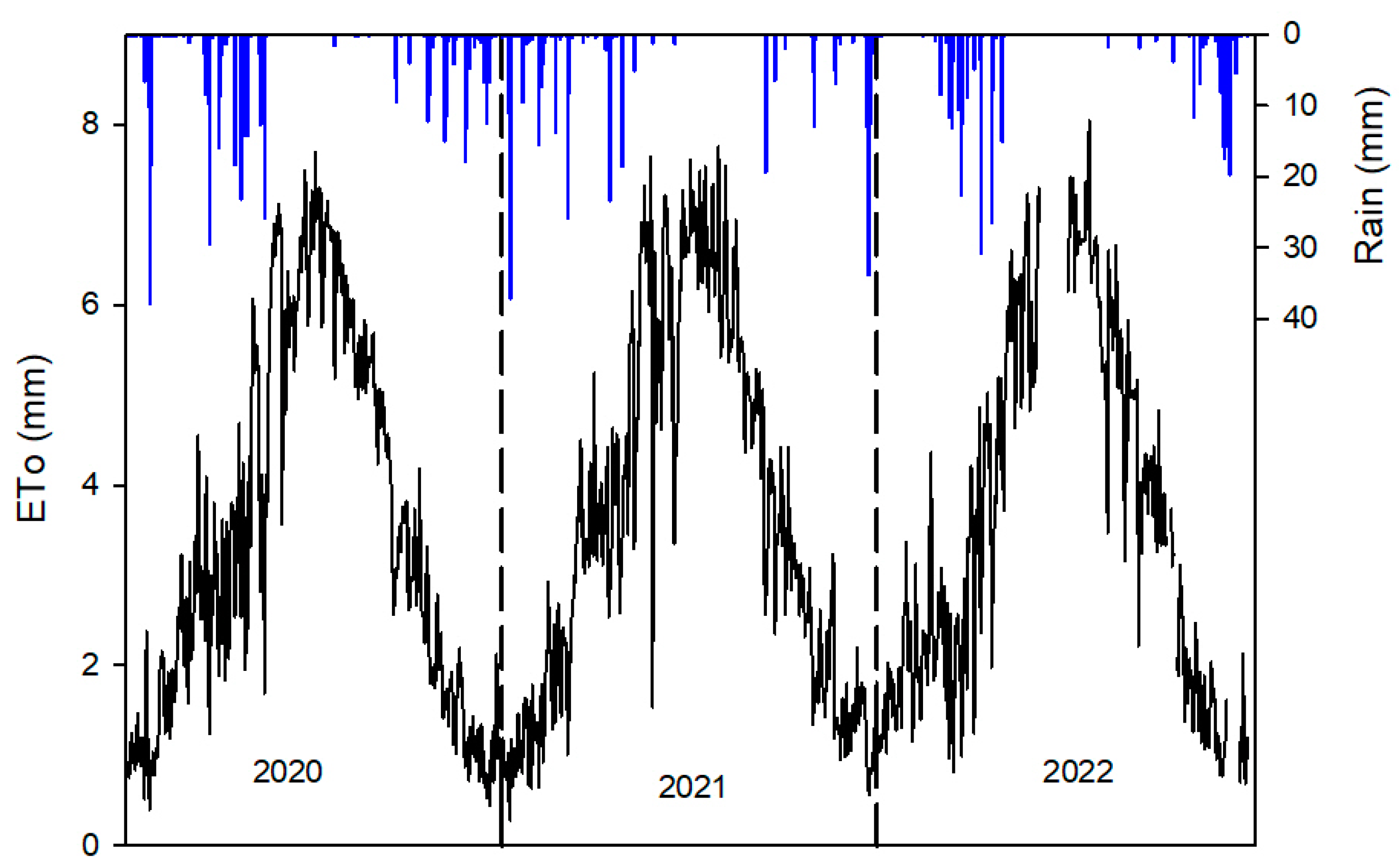
2. Materials and Methods

2.1. Description of the Site and the Treatments

Experiments were conducted during three consecutive seasons (from 2020 to 2022) in a hedgerow olive orchard (cv Manzanilla de Sevilla), 1.5 × 4 m distance in La Hampa experimental station in Coria del Río (near Seville, Spain, 37°17′ N, 6°3′ W, 30 m altitude). This orchard was planted in 2018 and the first yield (800 kg ha−1) was harvested in 2020. The soil was a sandy loam with more than 1 m depth. Climatic data were obtained from the Andalusian weather network, station “La Puebla” [26], about 6 km away from the experimental plot. Reference evapotranspiration (ETo) and rainfall during the experiment are presented in Figure 1.
The seasonal pattern of ETo and rainfall was typical of the Mediterranean basin. Winters were warm with minimum seasonal values of ETo. Spring–summer periods presented very high values of ETo, with maximum values greater than 7 mm day−1 but, most of the time, above 5 mm day−1 (Figure 1). Distribution of rain was concentrated in winter–early spring, with a common drought period during the rest of the season. Seasonal amounts of rains in the experimental period were lower than the 10 years average (534 mm, [27]) with values between 352 mm (in 2022) and 492 mm (in 2020).
The statistical design was completely randomized with six repetitions per treatment. Each plot contained five rows with thirteen trees each, and the three central rows were considered the measured trees. Every plot was irrigated with a drip system consisting of one single line for each tree row with drips 2.2 L h−1 and 0.5 m apart from each other. Treatments started from June 2020 due to the COVID-19 pandemic. Pit hardening was the period when irrigation restrictions were applied. The beginning of this phenological stage was estimated according to [28] and ended of the third week of August. Briefly, the beginning of the pit hardening occurred when the rate of longitudinal fruit growth was decreased [28]. Three different irrigation treatments were applied:
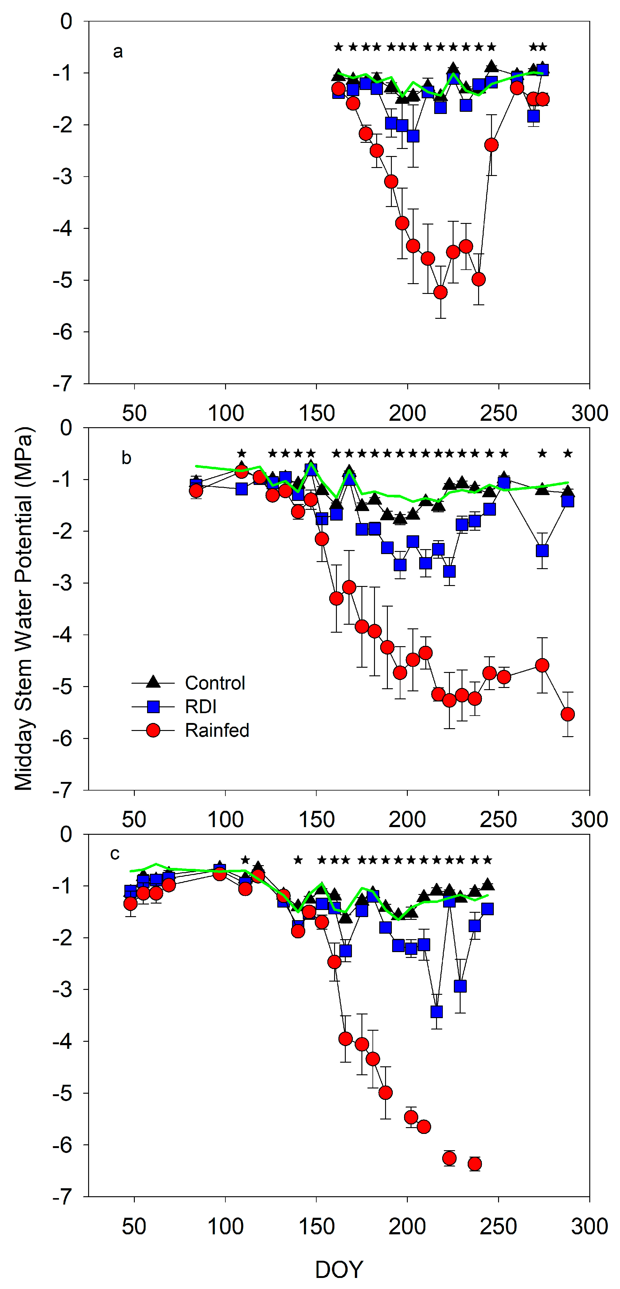
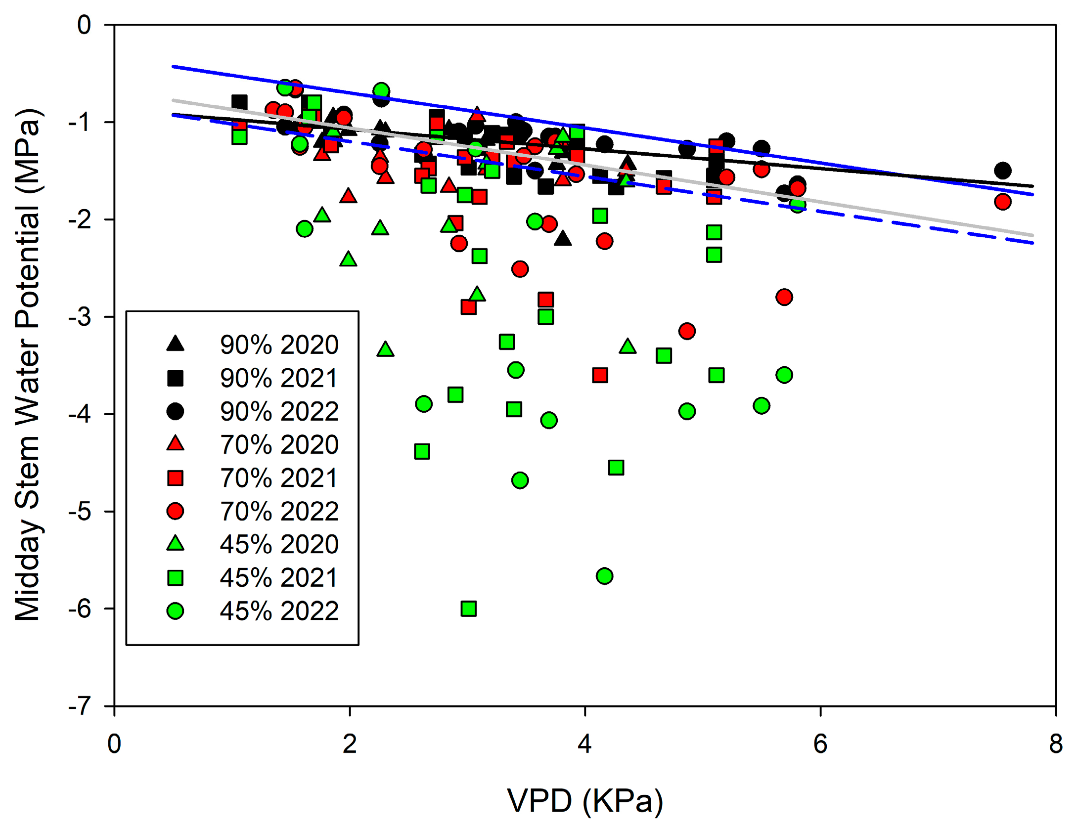
  • Control. Irrigation scheduling was based on the midday stem water potential (SWP) measurements. During the 2020 and 2021 seasons, the target was to maximize vegetative growth. Then, the amount of irrigation was estimated using the FAO 56 approach (crop coefficients (Kc) 0.55, reduction coefficient (Kr) 0.7). However, when the SWP was more negative than −1.0 MPa, the water applied increased to 175% crop evapotranspiration (Etc). The harvest yield in the 2021 season was considered similar to that of a mature orchard (nearly 10,000 kg ha−1). Therefore, irrigation scheduling changed in order to control vegetative growth. In the 2022 season, irrigation scheduling was used considering the same approach, but the SWP threshold was estimated based on the [12] baseline and it was lowered in 0.5 Mpa from pit hardening until harvest. The water applied per season was 553, 772, and 727 mm in 2020, 2021, and 2022, respectively.
  • Regulated deficit irrigation (RDI). The objective of this treatment was to apply mild or moderate water stress conditions, depending on the phenological stage. Irrigation scheduling was also based on the SWP measurements and on the comparison with the [12] baseline. Each plot was irrigated according to its SWP data. Trees were irrigated with 1 mm day−1 from the first date when the SWP was below the threshold, and the water applied increased by 2, 3, or 4 mm day−1 based on the distance to baseline. During the 2020 and 2021 seasons, in order to minimize the decrease in vegetative growth, the SWP threshold was the one obtained at the baseline and only during pit hardening it decreased to −2 MPa. In the 2022 season, the SWP threshold was the baseline value minus 0.5 MPa, but during pit hardening, it was minus 1.5 MPa. The water applied during the season was 267, 334, and 200 mm, respectively, in 2020, 2021, and 2022.
  • Rainfed. Trees were not irrigated from June 2020. Only in September of this season they were irrigated with 45 mm before harvest. No irrigation was applied during 2021 and 2022.
Yield production presented a very alternate bearing pattern, with very low fruits productions in the three treatments in 2020 and 2022 (between 500 and 1000 kg/ha) but high productions in 2021 for the irrigated treatments (around 9000 kg ha−1).

2.2. Description of Measurements

Water relations were characterized using the SWP and leaf conductance. The SWP was measured with the pressure bomb technique (PMS 1000, Albany, OR, USA) on fully expanded, healthy leaves that were covered around 2 h before the measurement was taken, and this was performed on one tree per plot at midday. Leaf conductance was measured at the same time as the SWP with a porometer (SC-1, Decagon, Pullman, WA, USA) on fully expanded sunny leaves. Both measurements were taken weekly. In order to determine the different SWP reference equations, the maximum value of leaf conductance every date was identify. The leaf conductance reduction was estimated as the ratio between the measurement on each plot and this maximum value. The SWP values used to determine the reference equations were the average of the SWP on the same date and in the same leaf conductance reduction interval. Three different levels of water stress were selected: values of leaf conductance between 90–100% of the daily maximum, 70–80%, and 45–55%.
Soil moisture was measured in each repetition with a portable FDR probe (HH2. Delta-T, Cambridge, UK) in 1 m depth. Access tubes were located in the irrigation line around 30 cm far from a drip. In addition, the percentage of soil cover was estimated at the beginning, after pruning, and at the end of each season. Three measurements of the horizontal dimensions in each plot were carried out with a scope.
Reference equations were estimated using linear regressions of these data vs. maximum daily temperature or maximum daily vapor pressure deficit (VPD). Meteorological data were obtained from the “La Puebla” Station [26], which is approximately 6 km away from the experimental station. Slopes of these regressions were compared to published baselines, for temperature [12] and for VPD [13] using a T-test (p < 0.05).

3. Results

Water relations were significantly affected in the three seasons. The midday stem water potential (SWP) showed extremely low values in the Rainfed treatment (Figure 2). Although the decrease in Rainfed trees was delayed in 2020 due to the COVID-19 pandemic (Figure 2a), the seasonal pattern was very similar with a fast decrease down to values between −5 and −6 MPa. During the 2020 season, Rainfed trees completely recovered in two weeks by the end of the experiment (Figure 2a), while in 2021 and 2022, the absence of rains kept the SWP values at very severe water stress levels (Figure 2b,c).
Significant differences between the Rainfed and Control were found early in the season, although at the beginning they were very similar. The Control trees presented a similar pattern in the three seasons. The SWP values in the Control were close to Corell’s baseline, reaching minimum values in mid-summer, at around DOY 200, in all seasons. Conversely, the RDI treatment trees showed a response that could be placed between the Rainfed and Control. Although the water status of the RDI was more similar to the Control, major differences between the RDI and Rainfed trees were delayed until severe water stress conditions of the Rainfed occurred at around −3 MPa. The RDI and Control trees presented significant differences but only on a few dates in the 2021 and 2022 seasons. Although these differences were not always important, Figure 2 shows clear periods of water stress in the RDI. The length of these periods and the level of water stress also changed for the different seasons. During 2020 (Figure 2a), the RDI presented the shortest period, around three weeks, while in the 2021 season it was the longest with more than two months (Figure 2b). The pattern of the SWP in the RDI was similar but not parallel to the Control, mainly during the 2022 season (Figure 2c).
Midday leaf conductance also presented significant differences throughout the season (Figure 3).
Leaf conductance in the Rainfed trees was considerably lower than the Control from mid-season but several weeks later than the SWP. In 2020, the rehydration period increased the rainfed leaf conductance to the same level compared to the Control and at a similar time compared to the SWP (Figure 2a), but no recovery was measured in the 2021 and 2022 seasons in rainfed trees. Differences between the Control and Rainfed treatments by the end of both seasons were smaller but still significant and likely related to a decrease in the Control values (Figure 3b,c). Control leaf conductance was very variable between seasons and days. Most Control measurements were around 400 mmol m−2 s−1 and tended to decrease by the end of all seasons. The RDI was an intermediate treatment between Rainfed and Control in all seasons, but with only a few significant differences (one or two per year) with the Control commonly around DOY 200. The RDI trees tended to greater leaf conductance values than the Rainfed ones in all seasons, but they were important only from DOY 200 in 2021 (Figure 3b).
The pattern of soil water extraction changed along the season with the irrigation management (Figure 4).
Figure 4 presented an example of the 2021 season (the high fruit load year) at three different dates: DOY 109 (around flowering), DOY 203 (mid-water stress period), and DOY 245 (just before harvest). At the beginning of the season, when small differences were found in the SWP or leaf conductance, the pattern of soil water uptake was different in the first 0.4 m. The Rainfed and RDI trees uptaked more water than the Control trees, but this water uptake was not observed in the deeper part of the profile. Such differences in water uptake were similar at DOY 203 (Figure 4b) when differences in the SWP were very clear. The RDI and Rainfed trees almost depleted the shallow part of the soil (until 0.4 m). Below that depth, there were no significant differences, but there was a trend of drier conditions in the Rainfed than in the RDI, which was near to the Control values. Finally, at DOY 245, at the end of the rehydration period, when the Rainfed presented significant, very severe SWP values but the RDI were recovered, the Rainfed profile was almost depleted. Although no significant differences were found because of the great variability, there was a clear increase in soil moisture in the profile at the RDI treatment that was very similar to the Control.
Figure 5 showed the pattern of the percentage of soil cover along the three seasons of the experiment. Soil cover data were obtained at the beginning of each season, after pruning, and at the end, after harvest. No significant differences were found in 2020 because irrigation treatments started after the main growth period. However, the Control trended to higher values than the Rainfed and RDI, and this fact better supports the water status conditions described with the rest of data.
The decrease in the Rainfed from 2021 season was produced for a more severe pruning to reduce the water stress compared to the others. No pruning was carried out in this treatment from this date. The percentage of soil cover in the Rainfed showed a very different pattern between seasons. In 2021, the highest fruit load season, no increase was measured while growth was significant during 2022 season. However, significant differences were found between the Rainfed and the rest of treatments in all dates from 2021. The decrease in the Control and RDI at the beginning of each season was related to pruning. On those dates, there were not significant differences between both, though the RDI was around five points lower than the Control. At the end of the 2021 and 2022 seasons, such differences in the percentage of soil cover were significant between both treatments. As in the Rainfed, during the 2022 season, the one with very low fruit load, RDI and Control showed maximum growth.
Figure 6 presents the relationship between the SWP and maximum daily temperature. Each season data were grouped according to their percentage of leaf conductance decrease. Table 1 shows the best fit of all data for the same interval of leaf conductance reduction. Data presented different levels of scattering in the three groups of conductance reduction, but this was smaller in the ones between 90% and 100% of maximum leaf conductance (Figure 6). The best fit of the 90–100% was linear with a low R2 but displayed a significant relationship with Tmax (Table 1). The slope of this relationship was not significantly different from Corell’s baseline, just slightly lower. Therefore, if they were considered as parallel, the equation in Table 1 would be around −0.3 MPa lower than Corell’s baseline (y-interception was 0 vs. 0.294 in Corell’s equation [12]). Data from 90–100% varied from values less negative than −1 to near −2 MPa (Figure 6).
The relationship of 70–80% leaf conductance reduction with Tmax was also significant but weaker than the ones from 90–100% (Table 1). These data presented a greater scattering than the previous group and varied from values less negative than −1 to slightly more negative than −3 MPa (Figure 6). Most data of 70–80% were less negative than −2 MPa (48 of 56 data). The slope of the regression, as in the previous group, was not significantly different from Corell’s baseline (Table 1). Finally, the group 45–55% of leaf conductance reduction had the greatest scattering in the SWP vs. Tmax relationship. The relationship between the SWP and Tmax were significant but very weak (Table 1). The slope of the equation was not significantly different to Corell’s baseline but tended clearly to more negative values. Data from this group, 45–55%, changed from less negative than −1 to around −6 MPa. The average of all data in this group was more negative than −2 MPa (20 of 48 data). According to [25], a SWP less negative than −1.5 MPa would be related to an isohydric respond. Then, the decrease in leaf conductance would be closely related to the evaporative demand instead of the water stress conditions. The relationship of the SWP vs. Tmax of 90–100% and 70–80% data more positive than −1.5 MPa improved the fit of the previous regression (ISO Tmax equation, Standard error and MSE in Table 1). The slope of this latter regression was significantly much lower than Corell’s one (Table 1, −0.023 vs. −0.046 [12]). Then, according to this equation, the SWP would be almost constant with the increase in Tmax (Figure 6).
The relationship of the SWP and maximum vapor pressure deficit (VPD) is shown in Figure 7, also with the same group of leaf conductance reduction than in Figure 6. The pattern of scattering in the three groups considered was the same as in the Tmax relationship. The group 90–100% presented the lowest variability and significantly lower slope than the [13] baseline. Conversely, data from the 70–80% group had a greater variability also in the VPD relationship. The relationship of this latter group was linear too, but with a low R2 (Table 1). The worse relationship was for the 45–55% group. The slope of this latter equation was not significantly different from the Shackel baseline, although it tended clearly to more negative values. Values from 90–100% and 70–80% more positive than −2 MPa presented a significant linear relationship (ISO VPD, Table 1). The slope of this latter equation was significantly less negative than the Schackel baseline slope. As in the Tmax relationship, the SWP variation with this latter equation was very small. The [12] baseline based on the VPD data is also presented in Figure 7. This equation is almost parallel to the Shackel estimation but approximately 0.3 MPa more negative.

4. Discussion

The pattern of the SWP and leaf conductance showed that the former was more sensitive to water stress under field conditions than the latter. Most of the seasons, the SWP decreased under conditions of water stress and recovered several weeks earlier than leaf conductance (Figure 2 and Figure 3). The differences between treatments were also greater in the SWP than in leaf conductance. These responses were reported in different irrigation works in young [21,29] and mature olive orchards [8,30]. However, this was not the case in other orchards, where significant lower leaf conductance was found at the beginning of the season, when the SWP was very positive and not different [5,31,32,33]. These changes in the sensitivity of leaf conductance would be related to two factors: percentage of roots in dry soil and isohydric response. Some authors [34] concluded that the delay in the recovery of leaf conductance from the water stress conditions was related to the volume of moist soil. Thus, partial root drying experiments showed that leaf conductance was affected by the presence of stress signals from roots, even with the same SWP [35]. But leaf stomata closure at the beginning of the season was not likely related to this. In this part of the season, when the SWP was still very positive (Figure 3) and likely vegetative growth was occurring in all treatments (Figure 5), this parameter would be linked to an isohydric response. Although traditionally plants were classified according to their isohydric and non-isohydric response [36], recent works suggested that some species could combine both. Some authors [25] suggested that both responses were possible in olive trees. At the beginning of the season, a great amount of soil water would promote the isohydric response, with a sharp decrease in leaf conductance before a small variation of the SWP [25]. Several authors reported this pattern in the leaf conductance vs. water potential relationship [14,15,17]. In the present work, these conditions could occur in the Control but were not clear in the RDI or Rainfed according to the soil moisture profile and differences in soil cover (Figure 4 and Figure 5). Differences in soil cover suggested a decrease in vegetative growth. These commonly occurred in olive trees before the SWP and leaf conductance affection [37]. The lack of response from leaf conductance to water deficit in some works, such as this one, would be likely related to data variability. According to several authors, transition from isohydric to non-isohydric would be between −1.5 and −2.3 MPa [14,15,25]. This change in the physiological response would affect water relations in the plant and the response to the environment.
Reference equations of the SWP changed when data considered the leaf conductance reduction (Figure 6 and Figure 7; Table 1). The scattering of the data increased with the decrease in leaf conductance, but relationships were usually weak (Table 1). Best fits in the 90–100% and 70–80% groups were parallel, and most of them were also parallel to the published reference equations (Table 1). All the above suggested that the same leaf conductance reduction would include a different position of the leaf conductance vs. water potential relationship, which increased the variability. Several authors reported that the SWP vs. leaf conductance relationship presented a great scattering, with values more positive than −2 MPa [14,15]. Only in the ISO data (Table 1, SWP more positive than −1.5 MPa and small leaf conductance reduction), the variability was small, and the reference equations presented a very slight slope, not parallel to the published baselines (Table 1). However, even in these ISO data, the SWP presented a meaningful relationship with evaporative demand (Temperature or VPD). Therefore, according to the current work, the selection of a constant value as a threshold for full irrigated conditions would not be advisable. Several authors reported a threshold of the SWP around −2 MPa or even more positive (−1.2 MPa, [7]) as indicator of full irrigated conditions [14,15]. However, these works assumed that the SWP measurements would be under isohydric conditions. This response in commercial orchards is likely to occur at the beginning of the season, but it would not be a common occurrence by mid-summer or dry spring, when part of the root zone could be under dry conditions [18,35]. Thus, reference equations that do not consider leaf conductance, such as [12] or [13], could be more appropriate for defining baseline equations than the ISO equation of this work or constant values.
Management of deficit irrigation based on the SWP baseline equations is not common. Some authors [13] suggested that baseline equations were defined as under “wet soil conditions”, and most of the time they would not be adequate for defining the target water status in a commercial orchard. Only under conditions that consider the tree growth as the main target of irrigation scheduling, the baseline could be the best reference for olive trees [13] because vegetative growth was more sensitive to water stress than the SWP [21,37]. In mature orchards, some authors [13] suggested equations parallel to the baseline for deficit irrigation scheduling. The current work claims that parallel equations occurred only until values around 0.5 MPa more negative than baselines (Figure 6 and Figure 7, Table 1). The SWP values below this threshold (baseline −0.5 MPa) would probably be better defined with constant values because of the great variability. In addition, according to the current results, these parallel equations would apply under moderate water stress conditions, when leaf conductance would be still not too limited. The estimation from Figure 6 and Figure 7 suggested that the SWP values were more positive than −2 MPa. On the other hand, the SWP reference equations could reduce their accuracy because of the variability or differences between locations. Although [12] suggested a single baseline, they presented differences between the fruit load conditions. Such differences were also reported in other plant water status indicators such as MDS [11]. Some authors [14] suggested three thresholds of the SWP on olive trees, which could facilitate the irrigation management up to −2 MPa, from −2 to −3.5 MPa and below −3.5 MPa. Further works would be advisable to check the limitations of irrigation manage based on the distance to the baseline. However, all these thresholds have to be considered just as a reference to study the real effect of water stress on the different processes in the tree. In fact, the yield response would be more complex and would probably include different processes and thresholds throughout the season. Some authors [8] suggested that table olive fruit growth would stop with the SWP below −2 MPa but would be reversible with an adequate rehydration. On the other hand, some authors [38] suggested that oil accumulation was very resistant to water stress, others suggested that a moderate water stress increased oil fruit yield [5,6,33], and finally a third group of authors considered that it decreased [16]. The comparison of the water stress level using the current reference equations could help to explain the differences between some of these results.

5. Conclusions

The SWP reference equations changed when the percentage of leaf conductance reduction was considered. These changes suggested parallel equations, which would decrease with the restriction of gas exchange. However, under conditions of severe water stress with a leaf conductance reduction between 45% and 55% the scattering was very high, and no clear linear relation was found. This suggests that water stress could be defined by the distance to a baseline but only in a narrow interval, around baselines minus 0.5 MPa. However, such approach could be very useful for establishing an accurate threshold in the most sensitive processes, such as the vegetative or fruit growth ones, or during periods very sensitive to water stress (flowering or fruit set).

Author Contributions

Conceptualization, A.M. and M.-J.M.-P.; methodology, M.S.-P., M.C. and P.C.-V.; formal analysis, M.S.-P. and A.M.; investigation, M.S.-P., M.C., P.C.-V., A.M. and M.-J.M.-P.; writing—original draft preparation, M.S.-P. and A.M.; writing—review and editing, M.C. and M.-J.M.-P.; project administration, A.M.; funding acquisition, M.C., A.M. and M.-J.M.-P. All authors have read and agreed to the published version of the manuscript.

Funding

This research was funded by Junta de Andalucía and FEDER, grant number P20-00492. Marta Sánchez-Piñero held a pre-doctoral fellowship from the University f Seville (VI-PPITUS).

Data Availability Statement

Data will be available at idus.us.es.

Acknowledgments

This research was supported by the Junta de Andalucía and the Fondo Europeo de Desarrollo (FEDER) project P20_00492. Marta Sánchez-Piñero held a pre-doctoral contract from the University f Seville (VI-PPITUS). Authors wish to thank Finca La Hampa for their helpful assistance during the experiment, and, in particular, Ignacio Girón.

Conflicts of Interest

The authors declare no conflict of interest.

References

  1. MAPA 2023. Yearbook of the Spanish Agriculture Ministry (Several Years). Available online: https://www.mapa.gob.es/es/estadistica/temas/publicaciones/anuario-de-estadistica/default.aspx (accessed on 15 March 2023).
  2. Hsiao, T.C. Measurements of plant water status. In Irrigation of Agricultural Crops; Steward, B.A., Nielsen, D.R., Eds.; American Society of Agronomy: Madison, WI, USA, 1990; pp. 243–280. [Google Scholar]
  3. Chalmers, D.J.; Wilson, I.B. Productivity of peach trees: Tree growth and water stress in relation to fruit growth and assimilate demand. Ann. Bot. 1978, 42, 285–294. [Google Scholar] [CrossRef]
  4. Steduto, P.; Hsiao, T.C.; Fereres, E.; Raes, D. Crop Yield Response to Water; FAO Irrigation and Drainage Paper 66; FAO: Rome, Italy, 2012. [Google Scholar]
  5. Moriana, A.; Orgaz, F.; Fereres, E.; Pastor, M. Yield responses of a mature olive orchard to water deficits. J. Am. Soc. Hortic. Sci. 2003, 128, 425–431. [Google Scholar] [CrossRef]
  6. Ben-Gal, A.; Ron, Y.; Yermiyahu, U.; Zipori, I.; Naoum, S.; Dag, A. Evaluation of regulated deficit irrigation strategies for oil olives: A case study for two modern Israeli cultivars. Agric. Water Manag. 2021, 245, 106577. [Google Scholar] [CrossRef]
  7. Moriana, A.; Pérez-López, D.; Prieto, M.H.; Ramírez-Santa-Pau, M.; Pérez-Rodriguez, J.M. Midday stem water potential as a useful tool for estimating irrigation requirements in olive trees. Agric. Water Manag. 2012, 112, 43–54. [Google Scholar] [CrossRef]
  8. Girón, I.F.; Corell, M.; Martín-Palomo, M.J.; Galindo, A.; Torrecillas, A.; Moreno, F.; Moriana, A. Feasibility of trunk diameter fluctuations in the scheduling of regulated deficit irrigation for table olive trees without references trees. Agric. Water Manag. 2015, 161, 114–126. [Google Scholar] [CrossRef]
  9. McCutchan, H.; Shackel, K.A. Stem-water potential as a sensitive indicator of water stress in Prune trees (Prunus domestica L. cv French). J. Amer. Soc. Hort. Sci. 1992, 117, 607–611. [Google Scholar] [CrossRef]
  10. Goldhamer, D.A.; Fereres, E. Irrigation scheduling of almond trees with trunk diameter sensors. Irrig. Sci. 2004, 23, 11–19. [Google Scholar] [CrossRef]
  11. Ortuño, M.F.; Conejero, W.; Moreno, F.; Moriana, A.; Intrigliolo, D.S.; Biel, C.; Mellisho, C.D.; Pérez-Pastor, A.; Domingo, R.; Ruiz-Sánchez, M.C.; et al. Could trunk diameter sensors be used in woody crops for irrigation scheduling? A review of current knowledge and future perspectives. Agric. Water Manag. 2010, 97, 1–11. [Google Scholar] [CrossRef]
  12. Corell, M.; Pérez-López, D.; Martín-Palomo, M.J.; Centeno, A.; Girón, I.; Galindo, A.; Moreno, M.M.; Moreno, C.; Memmi, H.; Torrecillas, A.; et al. Comparison of the water potential baseline in different locations. Usefulness for irrigation scheduling of olive orchards. Agric. Water Manag. 2016, 177, 308–316. [Google Scholar] [CrossRef]
  13. Shackel, K.; Moriana, A.; Marino, G.; Corell, M.; Perez-Lopez, D.; Martin-Palomo, M.J.; Caruso, T.; Marra, F.; Agüero-Alcaras, L.M.; Milliron, L.; et al. Establishing a reference baseline for midday stem water potential in olive and its use for plant-based irrigation management. Frontiers 2021, 12, 791711. [Google Scholar] [CrossRef]
  14. Marino, G.; Caruso, T.; Ferguson, L.; Marra, F.P. Gas exchanges and stem water potential define stress thresholds for efficient irrigation management in Olive (Olea europaea L.). Water 2018, 10, 342. [Google Scholar] [CrossRef]
  15. Ahumada-Orellana, L.; Ortega-Farias, S.; Poblete-Echeverría, C.; Searles, P.S. Estimation of stomatal conductance and stem water potential threshold values for water stress in olive trees (cv Arbequina). Irrig. Sci. 2019, 37, 461–467. [Google Scholar] [CrossRef]
  16. Hueso, A.; Trentacoste, E.R.; Junquera, P.; Gómez-Miguel, V.; Gómez del Campo, M. Differences in stem water potential during oil synthesis determine fruit characteristics and production but not vegetative growth or return bloom in an olive hedgerow orchard (cv Arbequina). Agric. Water Manag. 2019, 223, 105589. [Google Scholar] [CrossRef]
  17. Fernández, J.E. Understanding olive adaptation to abiotic stresses as a tool to increase crop performance. Environ. Exp. Bot. 2014, 103, 158–179. [Google Scholar] [CrossRef]
  18. Torres-Ruiz, J.M.; Diaz-Espejo, A.; Morales-Sillero, A.; Martín-Palomo, M.J.; Mayr, S.; Beikircher, B.; Fernández, J.E. Shoot hydraulic characteristics, plant water status and stomatal response in olive trees under different soil water conditions. Plant Soil 2013, 373, 77–87. [Google Scholar] [CrossRef]
  19. Perez-Martin, A.; Flexas, J.; Ribas-Carbó, M.; Bota, J.; Tomás, M.; Infante, J.M.; Diaz-Espejo, A. Interactive effects of soil waterdeficit and air vapour pressure deficit on mesophyll conductance to CO2 in Vitis vinifera and Olea europea. J. Exp. Bot. 2009, 60, 2391–2405. [Google Scholar] [CrossRef]
  20. Fernández, J.E.; Moreno, F. Water use by the olive tree. J. Crop Production 1999, 2, 101–162. [Google Scholar] [CrossRef]
  21. Moriana, A.; Fereres, E. Plant indicators for scheduling irrigation for young olive trees. Irrig. Sci. 2002, 21, 83–90. [Google Scholar] [CrossRef]
  22. Díaz-Espejo, A.; Walcroft, A.; Fernandez, J.E.; Hafidi, B.; Palomo, M.J.; Giron, I.F. Modelling photosynthesis in olive leaves under drought conditions. Tree Physiol. 2006, 26, 1445–1456. [Google Scholar] [CrossRef]
  23. Cuevas, M.V.; Torres-Ruiz, J.M.; Alvarez, R.; Jimenez, M.D.; Cuerva, J.; Fernandez, J.E. Assessment of trunk diameter variations derived índices as water stress indicators in mature olive tres. Agric. Water Manag. 2010, 97, 1293–1302. [Google Scholar] [CrossRef]
  24. Moriana, A.; Villalobos, F.J.; Fereres, E. Stomatal and photosynthetic responses of olive (Olea europaea L.) leaves to water deficit. Plant Cell Environ. 2002, 25, 395–405. [Google Scholar] [CrossRef]
  25. Díaz-Espejo, A.; Fernández, J.E.; Torres-Ruíz, J.M.; Rodríguez-Domínguez, C.M.; Pérez-Martin, A.; Hernández-Santana, V. The olive tree under water stress: Fitting the pieces of response mechanisms in the crop performance puzzle. In Water Scarcity and Sustainable Agriculture in Semiarid Environment. Tools, Strategies and Challenges for Woody Crops; García-Tejero, I., Martin-Zuago, V.H., Eds.; Academic Press, Elsevier: London, UK, 2018; pp. 439–480. [Google Scholar]
  26. SIAR 2023. Climatic Station Data in Spain. Available online: http://eportal.mapa.gob.es/websiar/SeleccionParametrosMap.aspx?dst=1 (accessed on 15 March 2023).
  27. AEMET 2023. Spanish Agency of Meteorology. Available online: http://www.aemet.es/es/serviciosclimaticos/datosclimatologicos/valoresclimatologicos?l=5783&k=undefined (accessed on 15 March 2023).
  28. Rapoport, H.F.; Pérez-López, D.; Hammami, S.B.M.; Aguera, J.; Moriana, A. Fruit pit hardening: Physical measurements during olive growth. Ann. Appl. Biol. 2013, 163, 200–208. [Google Scholar] [CrossRef]
  29. Gomez-del-Campo, M. Physiological and growth responses to irrigation of a newly established hedgerow olive orchard. HortScience 2010, 45, 809–814. [Google Scholar] [CrossRef]
  30. Moriana, A.; Pérez-López, D.; Gómez-Rico, A.; Salvador, M.D.; Olmedilla, N.; Ribas, F.; Fregapane, G. Irrigation scheduling for traditional, low density olive orchards: Water relations and influence on oil characteristics. Agric. Water Manag. 2007, 87, 171–179. [Google Scholar] [CrossRef]
  31. Agüero-Alcaras, L.M.; Rousseaux, M.C.; Searles, P.S. Responses of several soil and plant idicators to postharvestregulated deficit irrigation in olive trees and their potential for irrigation scheduling. Agric. Water Manag. 2016, 171, 10–20. [Google Scholar] [CrossRef]
  32. Padilla-Díaz, C.M.; Rodriguez-Dominguez, C.M.; Hernández-Santana, V.; Perez-Martin, A.; Fernandes, R.D.M.; Montero, A.; Garcia, J.M.; Fernández, J.E. Water status, gas Exchange and crop performance in a super high density olive orchard under deficit irrigation scheduled from leaf turgor measurements. Agric. Water Manag. 2018, 202, 241–252. [Google Scholar] [CrossRef]
  33. Corell, M.; Martín-Palomo, M.J.; Girón, I.; Andreu, L.; Galindo, A.; Centeno, A.; Pérez-López, D.; Moriana, A. Stem water potential-based regulated deficit irrigation scheduling for olive table trees. Agric. Water Manag. 2020, 242, 106418. [Google Scholar] [CrossRef]
  34. Pérez-López, D.; Gijón, M.C.; Moriana, A. Influence of irrigation rate on the rehydration of olive tree plantlets. Agric. Water Manag. 2008, 95, 1161. [Google Scholar] [CrossRef]
  35. Morales-Sillero, A.; García, J.M.; Torres-Ruiz, J.M.; Montero, A.; Sánchez-Ortiz, A.; Fernández, J.E. Is the productive performance of olive trees under localized irrigation affected by leaving some roots in drying soil? Agric. Water Manag. 2013, 123, 79–92. [Google Scholar] [CrossRef]
  36. Fereres, E. Variability in Adaptive Mechanisms to Water Deficits in Annual and Perennial Crop Plants. Actual. Bot. 1984, 131, 17–32. [Google Scholar] [CrossRef]
  37. Pérez-López, D.; Ribas, F.; Moriana, A.; Olmedilla, N.; De Juan, A. The effect of irrigation schedules on the water relations and growth of a young olive (Olea europaea L.) orchard. Agric. Water Manag. 2007, 89, 297–304. [Google Scholar] [CrossRef]
  38. López-Bernal, A.; Fernandes-Silva, A.A.; Vega, V.A.; Hidalgo, J.C.; León, L.; Testi, L.; Villalobos, F.J. A fruit growth approach to estimate oil content in olives. Eur. J. Agron. 2021, 123, 126206. [Google Scholar] [CrossRef]
Figure 1. Reference evapotranspiration (ETo) pattern, left, and rainfall pattern, right, throughout the three seasons of the experiment. Vertical lines delimit each year. Source: “La Puebla” Station [26].
Horticulturae 09 00563 g001
Figure 2. Midday stem water potential pattern throughout the (a) 2020, (b) 2021, and (c) 2022 seasons. Each point is the average of six measurements. The green solid line represents Corell’s baseline. Vertical bars are the standard error. Asterisks show the date when statistical differences were found (p < 0.05, Tukey Test).
Horticulturae 09 00563 g002
Figure 3. Midday leaf conductance pattern throughout (a) 2020, (b) 2021, and (c) 2022 seasons. Each point is the average of six measurements. Vertical bars are the standard error. Asterisks show the date when statistical differences were found (p < 0.05, Tukey Test).
Horticulturae 09 00563 g003
Figure 4. Soil moisture at different soil depths at three different dates of the 2021 season. (a) At the beginning of the season (DOY 109); (b) At mid-water stress period (DOY 203); (c) Just before harvest (DOY 245). Each symbol was the average of six data. Horizontal bars represent standard error. Asterisks indicated significant differences at the depth where they are located (p < 0.05, Tukey Test).
Horticulturae 09 00563 g004
Figure 5. Percentage of soil cover along the three experimental seasons. First data (03/2020) were the average of the orchard. Each symbol is the average of six data. Vertical bars represent standard error. Asterisks indicated the date when significant differences were found (p < 0.05, Tukey Test).
Horticulturae 09 00563 g005
Figure 6. Relationship between midday stem water potential and maximum daily temperature. Each symbol is the average of several data (different each date) in the same group of leaf conductance reduction. The black solid line represents the equation ISO (Table 1). The blue line represents the equation of [12] (solid) and plus 0.5 MPa (dash).
Horticulturae 09 00563 g006
Figure 7. Relationship between midday stem water potential and maximum daily VPD. Each symbol is the average of data in the same group of leaf conductance reduction. The black solid line represents the equation ISO (Table 1). The blue line represents the equation of [13] (solid) and plus 0.5 MPa (dash). The gray line represents the equation of [12].
Horticulturae 09 00563 g007
Table 1. Best fit of the relationship between midday stem water potential (SWP) vs. maximum daily temperature (Tmax, Figure 6) or vapor pressure deficit (VPD, Figure 7) with data from the groups 90–100%, 70–80%, 45–55%; and the two first groups more positive than −1.5 MPa (ISO)from Figure 6.
DatasetEquationData 1R2SDMSESig
90% TmaxSWP= −0.039 Tmax610.44 ***0.210.04No
70% TmaxSWP= −0.050 Tmax560.27 ***0.520.27No
45% TmaxSWP = −0.081 Tmax480.16 ***1.241.54No
ISO TmaxSWP= −0.468-0.023 Tmax840.39 ***0.160.03Yes
90% VPDSWP= −0.785-0.14 VPD610.43 ***0.210.04Yes
70% VPDSWP= −0.859-0.21 VPD560.21 ***0.540.30No
45% VPDSWP = −1.119-0.43 VPD480.15 **1.261.59No
ISO VPDSWP= −0.871-0.10 VPD840.34 ***0.170.03Yes
1 Data, amount of data in each equation; R2, coefficient of determination; SD, standard error; MSE, mean square error; Sig, slope significantly different from published baseline ([12] in Tmax and [13] in VPD); ***, p < 0.001: **, p < 0.01.
Disclaimer/Publisher’s Note: The statements, opinions and data contained in all publications are solely those of the individual author(s) and contributor(s) and not of MDPI and/or the editor(s). MDPI and/or the editor(s) disclaim responsibility for any injury to people or property resulting from any ideas, methods, instructions or products referred to in the content.

