

Estimation of the Total Nonstructural Carbohydrate Concentration in Apple Trees Using Hyperspectral Imaging

Department of Biosystem Engineering, Gyeongsang National University (Institute of Agriculture and Life Sciences), Jinju 52828, Republic of Korea
*
Author to whom correspondence should be addressed.
Horticulturae 2023, 9(9), 967; https://doi.org/10.3390/horticulturae9090967
Submission received: 21 July 2023
/
Revised: 23 August 2023
/
Accepted: 23 August 2023
/
Published: 25 August 2023
(This article belongs to the Topic Applications of Big Data and Machine Learning in Smart Agriculture)
Abstract
:The total nonstructural carbohydrate (TNC) concentration is an important indicator of the growth period and health of fruit trees. Remote sensing can be applied to monitor the TNC concentration in crops in a non-destructive manner. In this study, hyperspectral imaging from an unmanned aerial vehicle was applied to estimate the TNC concentration in apple trees. Partial least-squares regression, ridge regression, and Gaussian process regression (GP) were used to develop estimation models, and their effectiveness using selected key bands as opposed to full bands was evaluated in an effort to reduce computational costs and improve reproducibility. Nine key bands were identified, and the GP-based model using these key bands performed almost as well as the models using full bands. These results can be combined with previous studies on estimating the nitrogen concentration to provide useful information for more precise nutrient management to improve the yield and quality of apple trees.
1. Introduction
Carbohydrates comprise carbon, hydrogen, and oxygen atoms, and they are an important indicator of the yield and quality of fruit [1,2]. Total nonstructural carbohydrates (TNCs) comprise soluble sugars (i.e., fructose, sucrose, and glucose) and starch that are produced by photosynthesis in the leaves of a tree. Appropriate application of nitrogen fertilizer increases the leaf area, which increases the TNC supply and helps fruit grow larger in size [3,4]. The carbohydrate/nitrogen (C/N) ratio quantifies the relationship between TNCs produced by leaves and nitrogen absorbed from roots, and it differs according to the growth period and health of the tree. At a very low C/N ratio (i.e., N >> TNC), tree growth is weak, and flower buds do not form because of the lack of TNCs [5,6]. At low C/N ratios (i.e., N > TNC), tree growth is strong, but flower bud formation is low, and even if some flower buds form, fruiting is poor [7]. At C/N ratios close to or slightly above 1 (i.e., N ≅ TNC), tree growth is moderate, bud formation is high, and fruiting is sustained [8]. No specific value is given to the C/N ratio unless it is close to or slightly higher than 1. Finally, at high C/N ratios (i.e., N < TNC), tree growth is weak, flower bud formation is initially high but then decreases, and fruiting is poor [9]. For apple cultivation, a C/N ratio close to 1 is recommended.
Fertilization in a given year affects the next year because the nutrients produced by the leaves of the previous year are used by each organ of the tree, and the remainder is stored in the form of starch [10]. TNCs produced in the vegetative growth period (i.e., when buds sprout, roots develop, and leaves and stems grow) affect the reproductive growth period (i.e., when fruits ripen and mature qualitatively after flowering and pollination). In the vegetative growth period, TNCs are consumed by inorganic nitrogen. In the reproductive growth period, TNCs are not consumed by inorganic nitrogen, and nutrients are stored in the fruit [11]. Therefore, monitoring the TNC concentration of apple trees throughout the growing season is important for predicting the fruit yield and quality [12]. In particular, TNCs accumulate in fruit in earnest during the branching and fruit development periods until harvest [13]. Imbalances between carbon assimilation and nitrogen assimilation due to climatic conditions directly affect tree growth and fruit quality [14]. Especially in climates with heavy rain, carbon assimilation is hindered, and nitrogen assimilation is accelerated, which reduces the TNC concentration and results in overgrowth of the tree and exposure to various pests and diseases [15].
Remote sensing is widely applied to monitoring the growth status of vegetation under various soil and climatic conditions [16]. Continuous innovations and advances in remote sensing platforms have led to the emergence of unmanned aerial vehicles (UAVs) capable of collecting spectral imaging at low altitudes beneath clouds [17]. UAVs are relatively simple and inexpensive compared to other platforms such as satellites and aircraft, and they are more advantageous for quantitative estimation of nutrient levels in vegetation with high precision [18,19]. Various spectral imaging sensors can be mounted on UAVs. In particular, hyperspectral imaging has a high potential for monitoring the status of vegetation because it covers a wide range of central wavelengths (i.e., bands) from the visible light region to the invisible light region [20]. However, the disadvantages of hyperspectral imaging include the curse of dimensionality and a slow calculation time, which can be attributed to the vast amount of data. These limitations can be overcome by selecting key bands and excluding unnecessary or less important wavelengths [21,22]. Various methods have been proposed for selecting bands that are sensitive to specific factors useful for monitoring vegetation, such as principal component analysis and successive projection algorithm, but they generally suffer from problems such as low accuracy or complex processing [23]. First, since the distribution of data is assumed to be a Gaussian distribution, it is difficult to apply it if it is non-Gaussian or multi-Gaussian [24]. Second, it assumes the directions with large variance contain important information. In other words, since the axis is unconditionally shifted to the side where the covariance increases, it is difficult to describe that the result value has a structure that considers the characteristics of individual independent variables. Third, it assumes that the variables are correlated. That is, it is difficult to find principal components for uncorrelated variables. Finally, it is suitable for linear variables or relationships between variables [25]. In the case of non-linear characteristics, preprocessing, such as log transformation, is required. Recently, machine learning has been used to develop high-precision models and select key variables for monitoring vegetation status [26,27]. Most studies on using remote sensing and machine learning for the non-destructive monitoring of apple trees have been based on estimating the nitrogen content [23,28]. However, no studies have considered monitoring the TNC concentration despite its important role in determining fruit yield and quality.
In this study, the objective was to use UAV-based hyperspectral imaging to estimate the TNC concentration of apple trees in all growth periods. Estimation models were developed based on partial least-squares regression (PLS), ridge regression (RR), and Gaussian process regression (GP), and their performances with full bands and selected key bands were evaluated to determine the best-performing model.
2. Materials and Methods
2.1. Experimental Design
The study took place in an experimental field of the National Institute of Horticultural and Herbal Science of the Rural Development Administration in Wanju-gun, Jeollabuk-do. Three-year-old apple trees of the Hongro/M.9 cultivar were grown in pots containing a 5:4:1 ratio of horticultural bed soil, decomposed granite soil, and perlite. As shown in Figure 1, the pots were buried in the ground with 114 trees spaced 3 m apart horizontally and 2 m apart vertically. The 114 trees were divided into three equal groups of 38 trees with different types of nitrogen fertilization: excessive (171 g/year), moderate (43 g/year), and untreated (0 g/year). Fertilization was applied every week from 24 May to 14 August 2022. Hyperspectral images were acquired on 23 May, 3 June, 17 June, 4 July, 19 July, 28 July, 16 August, 7 September, and 21 September of that year. All images were acquired within 2 h of noon to minimize the influence of shadows.
2.2. Hyperspectral Image Acquisition and Processing
Images were acquired using a hyperspectral imaging sensor (MicroHSI 410 Shark, Corning Inc., Corning, New York, NY, USA) mounted on a UAV. The hyperspectral imaging sensor could measure 150 wavelengths in the range of 400–1000 nm with a field of view of 29.5°, and the size and weight were 13.7 cm × 8.74 cm × 7.04 cm and 0.68 kg, including the lens, respectively. The UAV was a quadcopter (Matrice 300 RTK, DJI Technology Inc., Shenzhen, China) with a size and weight of 96 cm × 103 cm × 43 cm and 6.3 kg, respectively. It had a maximum loading weight of 2.7 kg and a maximum flight time of about 45 min when the hyperspectral imaging sensor was mounted. The automatic flight of the UAV was controlled using DJI Pilot (DJI Technology Inc., Shenzhen, China), which is an Android-based dedicated software. The imaging area and flight plan were programmed in the Linux-based OS of the hyperspectral imaging sensor. Table 1 lists the flight and imaging specifications.
The obtained hyperspectral images were used to generate orthoimages with gyro correction and geometric correction using image processing software (ENVI 5.6, Exeils Visual Information Solutions, Boulder, CO, USA). The reflectances ρ of orthoimage were radiometrically corrected by dividing reflectances ρ of a 12% white reference board (Portable Fabric Target, Group 8 Technology Inc., Provo, UT, USA) to minimize the different light effects according to the time series:
The images were converted into normalized difference vegetation index images with reflectances ρ of 850 nm in the near-infrared (NIR) region and 677 nm in the red region:
To extract the spectral data of only the apple tree canopy, only the apple tree was designated as a region of interest. Figure 2 shows the extraction of the spectral data.
2.3. Total Nonstructural Carbohydrate Concentration
On each image acquisition date, 21 apple trees comprising seven apple trees from each nitrogen fertilization group were used to estimate the TNC concentration. Ten mature leaves were collected from each tree immediately after image acquisition. For each sample, 0.5 g of the leaves was ground and placed in a 500 mL Erlenmeyer flask. Then, 20 mL of 0.7 N HCL was added, and the mixture was heated in a hot water bath at 100 °C for 2 h and 30 min. Then, the solution was filtered through filter paper. Distilled water was added to obtain a total volume of 100 mL. After 3 mL of decomposition solution was boiled with 5 mL of dinitrosalicylic acid for 10 min, distilled water was added to obtain a total volume of 50 mL, and the color was developed. The absorbance of the solution was measured using an absorption spectrometer (UV0250 1PC, Shimadzu, Kyoto, Japan) at a wavelength of 550 nm. The TNC concentration was measured as a percentage of the dry mass in triplicate for each tree. The average values were used for the later estimation and analysis.
2.4. Analysis
A two-sample t-test was used to compare the TNC concentrations in the apple tree leaves according to the growing season and nitrogen fertilization. PLS-, RR-, and GP-based models for estimating the TNC concentration from the bands of spectral data were built in an agricultural data analysis platform (FinePro, Hortizen Co. Ltd., Jinju-si, Gyeongsangnam-do, Korea). The PLS-based model, a multivariate regression analysis method, was developed for comparison of estimation performance with the machine learning models. For each model, the dataset was divided into training (i.e., calibration) and test (i.e., prediction) datasets at a ratio of 7:3. The calibration and prediction models were cross-validated by setting k-fold to 5 as the validation model. The grid search method was used to identify the best parameters for each model (alpha for RR and GP and latent variables for PLS). The models were developed by sequentially applying latent variables from 1 to 15 in PLS and an alpha of 0.001, 0.01, 0.1, and 1 in RR and GP, and then the parameters of the model with the lowest MSE were selected. The possibility of reducing computational costs and improving reproducibility was considered by comparing the performances of models using the full bands and selected key bands [29]. The key bands were selected by comparing the R2 of the calibration (prediction) and validation models depending on the combination of bands listed through the rank of importance of each band using the variance importance in the projection method for the PLS-based model and the Shapley additive explanation (SHAP) method for the RR- and GP-based models. Summarizing the entire analysis flow through Figure 3, using reflectances in full bands of apple tree canopy as an independent variable and leaf carbohydrate concentration as a dependent variable, the models were developed using the divided training and test datasets. The key bands were selected by comparing the R2 of the models depending on the combination of bands listed through the rank of importance of each band. Finally, the most advantageous modeling method and parameters were also selected when using the key bands, compared with the model results using the full bands.
The model performance was evaluated according to the coefficient of determination (R2), root mean squared error (RMSE), and relative error (RE). The RMSE of the test dataset was denoted as the RMSE of the prediction (RMSEP). The RMSE and RE are calculated as follows:
where , is the average value of the TNC concentration, and n is the number of samples. RE represents the ratio of RMSE to the average vegetation growth.
2.4.1. Partial Least Squares Regression
PLS is an estimation technique that is an alternative to ordinary least squares regression, canonical correlation, or structural equation models and is particularly useful when the estimators are highly correlated or when the number of predictors exceeds the number of independent variables [30]. PLS combines the capabilities of principal components analysis and multiple regression analysis. First, latent factors explained by as much covariance as possible between the independent and dependent variables are extracted. The regression step then uses the decomposition of the independent variable to estimate the value of the dependent variable.
2.4.2. Ridge Regression
RR is a shrinkage method that minimizes the magnitude of coefficients by adding the squares of each coefficient based on the least squares method. In linear regression, the multicollinearity problem of independent variables is reduced in accuracy, and some information, including noise, is deleted to develop the optimal model [31].
2.4.3. Gaussian Process Regression
GP is a probabilistic approach of the Bayesian framework capable of addressing the complexity between test and training input values to its non-linear behavior [32]. GP, a family of kernel methods, assumes that a multidimensional Gaussian distribution process governs a set of possible latent functions and that likelihoods and observations shape before generating posterior stochastic estimates [33].
2.4.4. Variance Importance in Projection
The variance importance in the projection value is calculated as the importance of each predictor, reflecting the weighted sum of squares of the PLSR weights [29]. The VIP can synthetize the contributions of the predictor and response variables, and the variables with a VIP value greater than 0.8 or 1 are considered significant [34].
2.4.5. Shapley Additive Explanation
SHAP explores and explains the relationship between input variables and output values of a complex machine learning model through Shapley values. The Shapley value can be obtained by the change due to the addition or removal of the corresponding variable in the combination of several variables, and through the change, both positive and negative influences of each input variable can be calculated [35]. The SHAP technique has the disadvantage of taking a long time to calculate the results because of the calculation method but has the advantage of measuring the influence of variables on the estimated value more accurately than the existing feature importance technique.
3. Results
3.1. Basic Analysis of the Total Nonstructural Carbohydrate Concentration
Table 2 presents the results of the two-sample t-test in terms of the mean and standard deviation of the TNC concentration depending on the nitrogen fertilization and growing season. Among the fertilization groups, the TNC concentration only showed significant differences on July 28 and September 21. The group with excessive nitrogen fertilization tended to have a lower TNC concentration than the other groups [36]. Regardless of the fertilization group, the TNC concentration was higher after mid-July than before mid-July, which corresponds to the transition from the fruit development and branching periods to the reproductive growth period [37].
3.2. Reflectance Curves
Figure 4 shows the reflectance of the apple tree canopies in each band. The visible light region (400 nm–680 nm) had the lowest reflectance, which is because it corresponds to the wavelengths that are absorbed by chlorophyll in vegetation for photosynthesis [38]. In this region, a peak was observed at 550 nm, which corresponds to green. The reflectance increased rapidly in the red-edge region (680–750 nm) and stabilized in the near-infrared (NIR) region (>750 nm). The reflectance decreased rapidly above 900 nm, which is because wavelengths in this range are absorbed by moisture in the vegetation. These results confirmed that the hyperspectral imaging sensor obtained reflectance curves typical for vegetation.
3.3. Estimation Performance of the Models with Full Bands
Table 3 presents the performances of the models at estimating the TNC concentration using full bands. With the training dataset, all models achieved a calibration performance of R2 ≥ 0.71, RMSE ≤ 1.32%, and RE ≤ 6.91% and a validation performance of R2 ≥ 0.59, RMSE ≤ 1.57%, and RE ≤ 8.22%. With the test dataset, all models achieved a prediction performance of R2 ≥ 0.70, RMSEP ≤ 1.41%, and RE ≤ 7.43% and a validation performance of R2 ≥ 0.57, RMSEP ≤ 1.68%, and RE ≤ 8.86%. For the model parameters, the RR- and GP-based models were set to an alpha value of 0.001, and the PLS-based model was set to a latent variable of 8. With full bands, all models showed no significant difference in estimation performance between the training and test datasets. The models were not considered overfitted because the difference in performance between calibration (or prediction) and validation was not large. These results indicate the possibility of an estimation model being developed with high reproducibility in other spatiotemporal dimensions in the future.
3.4. Estimation Performance of the Models with Key Bands
Table 4 presents the nine selected key bands for each model, which were then used to compare their estimation performances of the TNC concentration using full bands. For the PLS-based model, two bands in the blue region (401 and 405 nm), four bands in the red-edge region (697, 701, 705, and 709 nm), and three bands in the NIR region (758, 762, and 766 nm) were selected. In contrast, the same bands were selected in the NIR region between 754 and 874 nm for both the RR- and GP-based models.
Table 5 presents the estimation performances of the models. With the training dataset, all models achieved the same performance with the key bands as with the full bands. In contrast, the estimation performance differed with the test dataset. The PLS-based model achieved R2 ≤ 0.30, RMSE ≥ 2.16%, and RE ≥ 11.4%. The RR-based model achieved R2 ≤ 0.63, RMSE ≥ 1.56%, and RE ≥ 8.23%. The GP-based model achieved R2 ≤ 0.68, RMSE ≥ 1.46%, and RE ≥ 7.70%. The GP-based model used an alpha value of 0.001, and the PLSR model used a latent variable of 7. The models were not considered overfitted because the difference in performance between the calibration (or prediction) and validation was not large. The RR-and GP-based models performed better than the PLS-based model, which may be because the selected key bands were all in the NIR region. In particular, the GP-based model performed the best. Figure 5 plots the TNC estimation results of the GP-based model using full and key bands. The linear trends were similar to the full bands and key bands for samples spanning low, medium, and high TNC concentrations.
4. Discussion
4.1. Relationship between Selected Bands and Total Nonstructural Carbohydrate Concentration
Table 6 presents the R2 values of the GP-based model according to the number of bands (5–15) used to estimate the TNC concentration. With the training dataset, the model had R2 values of 0.73 for calibration and 0.59 for validation, regardless of the number of bands. With the test dataset, the model had R2 ≤ 0.56 for both prediction and validation at 12–15 bands. Using 9–11 bands increased the R2 value to ≥0.63. Decreasing the number of bands to less than eight caused a gradual decrease in the R2 value. In terms of computational cost, selecting a smaller number of bands for a similar estimation performance is more performance [39]. Therefore, the nine bands in Table 4 were selected for further analysis of the estimation performance of the GP-based model.
Figure 6 shows the SHAP values, indicating the importance of each band to the estimation performance of the GP-based model. Figure 6a shows the results for a model using 12 bands: 754, 762, 778, 790, 814, 818, 826, 850, 854, 862, 866, and 874 nm. The SHAP values were higher at 754, 778, and 790 nm than at bands after 800 nm. When nine bands were selected (Figure 6c), 790 nm was excluded along with 814 and 818 nm, despite their relatively high importance. The SHAP values increased at 850 and 854 nm and remained high at 778 nm. The SHAP values of each band differed depending on the number of bands and their combinations. Thus, even if a certain band had a high SHAP value with twelve bands, if the SHAP value decreased with nine bands, then it should be excluded from model development. Figure 6b shows the results using 10 bands, which included 818 nm. The SHAP distribution and R2 value (Table 6) were similar to those at nine bands. With six bands, 850 and 854 nm were excluded, which greatly affected the estimation performance and lowered the R2 value to ≤0.45. These results confirmed that the bands at 850 and 854 nm had a significant influence on the estimation of the TNC concentration in apple trees. In addition, the bands at 754, 762, 778, 826, 862, 866 and 874 nm were selected as key to the estimation performance.
4.2. Comparison with Related Studies
GP has previously been applied to estimating the growth and disease of various trees [40,41,42], but this study is the first to apply it to estimating the nutritional status of apple trees. Previous studies that have combined remote sensing with hyperspectral imaging estimated the nitrogen content of leaves to monitor the nutritional status, either on the ground [43] or in the air [23]. Estimations using selected key bands have been conducted with multivariate linear regression (i.e., PLS) and machine learning regression (i.e., support vector machine) and achieved R2 values of 0.78 on the ground and 0.67 in the air. The selected bands for estimating the nitrogen content and TNC concentration differ. While the key bands for estimating the TNC concentration were all in the NIR region, the key bands for estimating the nitrogen content often fell in the visible light region, except for 705 nm in the red-edge region. Nitrogen is a major component of proteins, nucleic acids, and chlorophyll in plants, and it is closely related to photosynthesis [44]. Most of the visible light region is absorbed and reflected by chloroplasts, which are most numerous in the palisade tissue, and this may have influenced the selection of key bands. In fact, Yu et al. selected key bands in the visible light region to estimate the chlorophyll content in apple tree leaves [45]. In trees, TNCs include glucose, which is produced by photosynthesis, and starch, which is how numerous glucose molecules are stored [46]. Most of the starch is stored in the chloroplasts of the leaves during the day; at night, it is converted into sugar and transported to each part of the plant [47]. Thus, bands in the NIR region may be advantageous for monitoring molecules stored inside the chloroplast around noon, which coincides with the hyperspectral imaging acquisition in this study [48,49]. The developed model in this study for estimating the TNC concentration can be combined with existing models for estimating the nitrogen content to improve the monitoring and health management of apple trees for improved fruit yield and quality. For example, Figure 7 shows a time-series nutrient map of the TNC concentration of the apple trees in this study estimated by the GP-based model using nine key bands.
5. Conclusions
This study investigated the feasibility of using UAV-based hyperspectral imaging to estimate the TNC concentration of apple tree leaves. A GP-based model was obtained that demonstrated a similar estimation performance with nine key bands compared to full bands. The results indicated that using bands in the NIR region is advantageous for estimating TNC molecules stored inside chloroplasts. In order to be reproduced in actual orchards, there is still a task to verify and expand this TNC estimation model under various environmental conditions. In addition, for precise tree nutrition management, an integrated study to verify the yield and quality of apples according to the health status of apple trees in more detail by estimating nitrogen and TNC at the same time should be conducted.
Author Contributions
Conceptualization, Y.-S.K. and C.-S.R.; methodology Y.-S.K.; validation, C.-S.R.; formal analysis, Y.-S.K. and K.-S.P.; investigation, E.-R.K. and J.-C.J.; writing original draft preparation, Y.-S.K.; writing—review and editing, Y.-S.K. and C.-S.R.; supervision Y.-S.K.; funding acquisition, Y.-S.K. and C.-S.R.; All authors have read and agreed to the published version of the manuscript.
Funding
This research was funded by the National Institute of Crop Science, Rural Development Administration (Project name: Development of image-based physiological diagnosis technique for apple and pear trees and Project number: PJ0156572023).
Data Availability Statement
Not applicable.
Acknowledgments
The authors appreciate all staff who helped with this study in the Fruit Research Division of the National Institute of Horticultural and Herbal Science, Rural Development Administration, Korea.
Conflicts of Interest
The authors declare no conflict of interest.
References
- Aparadh, V.T.; Karadge, B.A. Comparative carbohydrates status in leaf developmental stages of Cleome species. Int. J. Pharm. Sci. Rev. Res. 2012, 14, 130–132. [Google Scholar]
- Larson, J.E.; Perkins-Veazie, P.; Ma, G.; Kon, T.M. Quantification and prediction with near infrared spectroscopy of carbohydrates throughout apple fruit development. Horticulturae 2023, 9, 279. [Google Scholar] [CrossRef]
- Haller, M.H.; Magness, J.R. Relation of Leaf Area and Position to Quality of Fruity and to Bud Differentiation in Apples (No. 1488-2016-123788). Ph.D. Thesis, University of Maryland, College Park, MD, USA, 1933. [Google Scholar]
- Rutkowski, K.; Łysiak, G.P. Effect of nitrogen fertilization on tree growth and nutrient content in soil and cherry leaves (Prunus cerasus L.). Agriculture 2023, 13, 578. [Google Scholar] [CrossRef]
- Shaolan, H.E.; Lie, D.E.N.G.; Yiqin, L.I.; Rong, L. Effects of floral promotion or inhibition treatments on flowering of citrus trees and protein fractions in buds. J. Trop. Subtrop. Bot. 1998, 6, 124–130. [Google Scholar]
- Budiarto, R.; Poerwanto, R.; Santosa, E.; Efendi, D. Shoot manipulations improve flushing and flowering of mandarin citrus in Indonesia. J. Appl. Hortic. 2018, 20, 112–118. [Google Scholar] [CrossRef]
- Goldschmidt, E.E.; Golomb, A. The carbohydrate balance of alternate-bearing citrus trees and the significance of reserves for flowering and Fruiting1. J. Am. Soc. Hortic. Sci. 1982, 107, 206–208. [Google Scholar] [CrossRef]
- Goldschmidt, E.E. Carbohydrate supply as a critical factor for citrus fruit development and productivity. HortScience 1999, 34, 1020–1024. [Google Scholar] [CrossRef]
- Zwieniecki, M.A.; Davidson, A.M.; Orozco, J.; Cooper, K.B.; Guzman-Delgado, P. The impact of non-structural carbohydrates (NSC) concentration on yield in Prunus dulcis, Pistacia vera, and Juglans regia. Sci. Rep. 2022, 12, 4360. [Google Scholar] [CrossRef]
- Bustan, A.; Avni, A.; Lavee, S.; Zipori, I.; Yeselson, Y.; Schaffer, A.A.; Riov, J.; Dag, A. Role of carbohydrate reserves in yield production of intensively cultivated oil olive (Olea europaea L.) trees. Tree Physiol. 2011, 31, 519–530. [Google Scholar] [CrossRef]
- Rossouw, G. Grapevine Carbohydrate and Nitrogen Allocation during Berry Maturation: Implications of Source-Sink Relations and Water Supply. Ph.D. Thesis, Charles Sturt University, Bathurst, Australia, 2017. [Google Scholar]
- Suárez, L.; Zarco-Tejada, P.J.; González-Dugo, V.; Berni, J.A.J.; Sagardoy, R.; Morales, F.; Fereres, E. Detecting water stress effects on fruit quality in orchards with time-series PRI airborne imagery. Remote Sens. Environ. 2010, 114, 286–298. [Google Scholar] [CrossRef]
- Skarpe, C.; Hester, A.J. Plant traits, browsing and gazing herbivores, and vegetation dynamics. Ecol. Stud. 2008, 195, 217–261. [Google Scholar]
- Demestihas, C.; Plénet, D.; Génard, M.; Raynal, C.; Lescourret, F. Ecosystem services in orchards. A review. Agron. Sustain. Dev. 2017, 37, 1–21. [Google Scholar] [CrossRef]
- Albrigo, L.G.; Buker, R.S.; Burn, J.K.; Castle, W.S.; Futch, S.; McCoy, C.W.; Muraro, R.P.; Rogers, M.E.; Syvertsen, J.P.; Timmer, L.W.; et al. The impact of four hurricanes in 2004 on the Florida citrus industry: Experiences and lessons learned. Proc. Fla. State Hortic. Soc. 2005, 118, 66–74. [Google Scholar]
- Sishodia, R.P.; Ray, R.L.; Singh, S.K. Applications of remote sensing in precision agriculture: A review. Remote Sens. 2020, 12, 3136. [Google Scholar] [CrossRef]
- Raj, R.; Kar, S.; Nandan, R.; Jagarlapudi, A. Precision agriculture and unmanned aerial Vehicles (UAVs). In Unmanned Aerial Vehicle: Applications in Agriculture and Environment; Springer: Berlin/Heidelberg, Germany, 2020; pp. 7–23. [Google Scholar]
- Ashapure, A.; Jung, J.; Chang, A.; Oh, S.; Yeom, J.; Maeda, M.; Maeda, A.; Dube, N.; Landivar, J.; Hague, S.; et al. Developing a machine learning based cotton yield estimation framework using multi-temporal UAS data. ISPRS J. Photogramm. 2020, 169, 180–194. [Google Scholar] [CrossRef]
- Hunt Jr, E.R.; Daughtry, C.S.T. What good are unmanned aircraft systems for agricultural remote sensing and precision agriculture? Int. J. Remote Sens. 2018, 39, 5345–5376. [Google Scholar] [CrossRef]
- Kumar, L.; Schmidt, K.; Dury, S.; Skidmore, A. Imaging spectrometry and vegetation science. In Imaging Spectrometry: Basic Principles and Prospective Applications; Springer: Berlin/Heidelberg, Germany, 2002; pp. 111–155. [Google Scholar]
- Rashwan, S.; Dobigeon, N. A split-and-merge approach for hyperspectral band selection. IEEE Geosci. Remote Sens. Lett. 2017, 14, 1378–1382. [Google Scholar] [CrossRef]
- Sawant, S.; Manoharan, P. Hyperspectral band selection based on metaheuristic optimization approach. Infrared Phys. Technol. 2020, 107, 103295. [Google Scholar] [CrossRef]
- Li, M.; Zhu, X.; Li, W.; Tang, X.; Yu, X.; Jiang, Y. Retrieval of nitrogen content in apple canopy based on unmanned aerial vehicle hyperspectral images using a modified correlation coefficient method. Sustainability 2022, 14, 1992. [Google Scholar] [CrossRef]
- Huang, J.; Yan, X. Gaussian and non-Gaussian double subspace statistical process monitoring based on principal component analysis and independent component analysis. Ind. Eng. Chem. Res. 2015, 54, 1015–1027. [Google Scholar] [CrossRef]
- Malthouse, E.C. Limitations of nonlinear PCA as performed with generic neural networks. IEEE Trans. Neural Netw. 1998, 9, 165–173. [Google Scholar] [CrossRef] [PubMed]
- Feng, Z.H.; Wang, L.Y.; Yang, Z.Q.; Zhang, Y.Y.; Li, X.; Song, L.; He, L.; Duan, J.Z.; Feng, W. Hyperspectral monitoring of powdery mildew disease severity in wheat based on machine learning. Front. Plant Sci. 2022, 13, 828454. [Google Scholar] [CrossRef] [PubMed]
- Han, L.; Yang, G.; Dai, H.; Xu, B.; Yang, H.; Feng, H.; Li, Z.; Yang, X. Modeling maize above-ground biomass based on machine learning approaches using UAV remote-sensing data. Plant Methods 2019, 15, 10. [Google Scholar] [CrossRef]
- Li, W.; Zhu, X.; Yu, X.; Li, M.; Tang, X.; Zhang, J.; Xue, Y.; Zhang, C.; Jiang, Y. Inversion of nitrogen concentration in apple canopy based on UAV hyperspectral images. Sensors 2022, 22, 3503. [Google Scholar] [CrossRef] [PubMed]
- Kang, Y.S.; Jang, S.H.; Park, J.W.; Song, H.Y.; Ryu, C.S.; Jun, S.R.; Kim, S.H. Yield prediction and validation of onion (Allium cepa L.) using key variables in narrowband hyperspectral imagery and effective accumulated temperature. Comput. Electron. Agric. 2020, 178, 105667. [Google Scholar] [CrossRef]
- Mateos-Aparicio, G. Partial least squares (PLS) methods: Origins, evolution, and application to social sciences. Commun. Stat.-Theory Methods 2011, 40, 2305–2317. [Google Scholar] [CrossRef]
- Ji, S.; Gu, C.; Xi, X.; Zhang, Z.; Hong, Q.; Huo, Z.; Zhao, H.; Zhang, R.; Li, B.; Tan, C. Quantitative monitoring of leaf area index in rice based on hyperspectral feature bands and ridge regression algorithm. Remote Sens. 2022, 14, 2777. [Google Scholar] [CrossRef]
- Arefi, A.; Sturm, B.; von Gersdorff, G.; Nasirahmadi, A.; Hensel, O. Vis-NIR hyperspectral imaging along with Gaussian process regression to monitor quality attributes of apple slices during drying. LWT 2021, 152, 112297. [Google Scholar] [CrossRef]
- Verrelst, J.; Rivera, J.P.; Gitelson, A.; Delegido, J.; Moreno, J.; Camps-Valls, G. Spectral band selection for vegetation properties retrieval using Gaussian processes regression. Int. J. Appl. Earth Obs. Geoinf. 2016, 52, 554–567. [Google Scholar] [CrossRef]
- Stellacci, A.M.; Castrignanò, A.; Troccoli, A.; Basso, B.; Buttafuoco, G. Selecting optimal hyperspectral bands to discriminate nitrogen status in durum wheat: A comparison of statistical approaches. Environ. Monit. Assess. 2016, 188, 1–15. [Google Scholar] [CrossRef]
- Kannangara, K.P.M.; Zhou, W.; Ding, Z.; Hong, Z. Investigation of feature contribution to shield tunneling-induced settlement using Shapley additive explanations method. J. Rock Mech. Geotech. Eng. 2022, 14, 1052–1063. [Google Scholar] [CrossRef]
- Leite, R.G.; Cardoso, A.D.S.; Fonseca, N.V.B.; Silva, M.L.C.; Tedeschi, L.O.; Delevatti, L.M.; Ruggieri, A.C.; Reis, R.A. Effects of nitrogen fertilization on protein and carbohydrate fractions of Marandu palisadegrass. Sci. Rep. 2021, 11, 14786. [Google Scholar] [CrossRef]
- Imada, S.; Tako, Y. Seasonal accumulation of photoassimilated carbon relates to growth rate and use for new aboveground organs of young apple trees in following spring. Tree Physiol. 2022, 42, 2294–2305. [Google Scholar] [CrossRef] [PubMed]
- Peñuelas, J.; Filella, I. Visible and near-infrared reflectance techniques for diagnosing plant physiological status. Trends Plant Sci. 1998, 3, 151–156. [Google Scholar] [CrossRef]
- Sun, W.; Du, Q. Hyperspectral band selection: A review. IEEE Geosci Remote Sens. Mag. 2019, 7, 118–139. [Google Scholar] [CrossRef]
- Hultquist, C.; Chen, G.; Zhao, K. A comparison of Gaussian process regression, random forests and support vector regression for burn severity assessment in diseased forests. Remote Sens. Lett. 2014, 5, 723–732. [Google Scholar] [CrossRef]
- Mutanen, T.; Sirro, L.; Rauste, Y. Tree height estimates in boreal forest using Gaussian process regression. In Proceedings of the IEEE International Geoscience and Remote Sensing Symposium (IGARSS) 2016, Beijing, China, 10–15 July 2016; IEEE: Piscataway, NJ, USA, 2016; pp. 1757–1760. [Google Scholar]
- Xie, R.; Darvishzadeh, R.; Skidmore, A.K.; Heurich, M.; Holzwarth, S.; Gara, T.W.; Reusen, I. Mapping leaf area index in a mixed temperate forest using Fenix airborne hyperspectral data and Gaussian processes regression. Int. J. Appl. Earth Obs. Geoinf. 2021, 95, 102242. [Google Scholar] [CrossRef]
- Ye, X.; Abe, S.; Zhang, S. Estimation and mapping of nitrogen content in apple trees at leaf and canopy levels using hyperspectral imaging. Precis Agric. 2020, 21, 198–225. [Google Scholar] [CrossRef]
- Ohyama, T. Nitrogen as a major essential element of plants. Nitrogen Assim. Plants 2010, 37, 1–17. [Google Scholar]
- Yu, R.; Zhu, X.; Cao, S.; Xiong, J.; Wen, X.; Jiang, Y.; Zhao, G. Estimation of chlorophyll content in apple leaves based on imaging spectroscopy. J. Appl. Spectrosc. 2019, 86, 457–464. [Google Scholar] [CrossRef]
- Streb, S.; Zeeman, S.C. Starch metabolism in Arabidopsis. Arab. Book Am. Soc. Plant Biol. 2012, 10, e0160. [Google Scholar] [CrossRef] [PubMed]
- Aluko, O.O.; Li, C.; Wang, Q.; Liu, H. Sucrose utilization for improved crop yields: A review article. Int. J. Mol. Sci. 2021, 22, 4704. [Google Scholar] [CrossRef]
- Giraldo, J.P.; Wu, H.; Newkirk, G.M.; Kruss, S. Nanobiotechnology approaches for engineering smart plant sensors. Nat. Nanotechnol. 2019, 14, 541–553. [Google Scholar] [CrossRef] [PubMed]
- Zhang, Q.; Ying, Y.; Ping, J. Recent advances in plant nanoscience. Adv. Sci. 2022, 9, e2103414. [Google Scholar] [CrossRef] [PubMed]
Figure 1.
Apple orchard with excessive (blue), moderate (yellow), and untreated (red) nitrogen fertilization.
Figure 1.
Apple orchard with excessive (blue), moderate (yellow), and untreated (red) nitrogen fertilization.
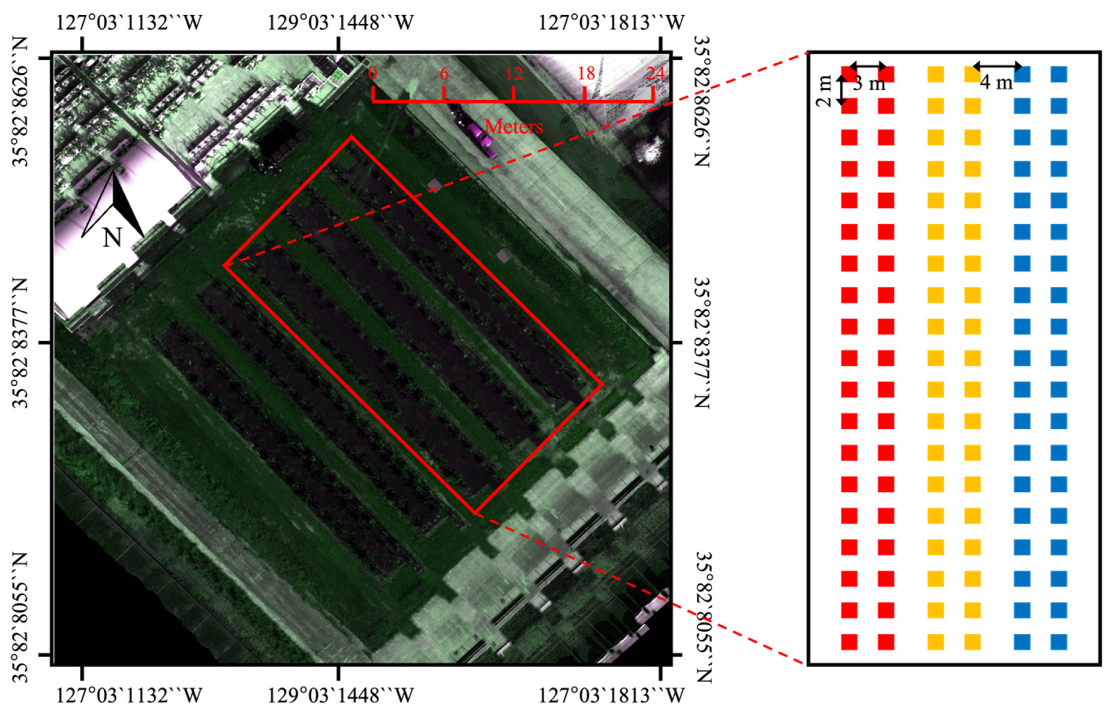
Figure 2.
Hyperspectral image processing procedure: (a) raw RGB image; (b) conversion to the normalized difference vegetation index; (c) extraction of apple tree canopies; (d) extraction of individual canopies.
Figure 2.
Hyperspectral image processing procedure: (a) raw RGB image; (b) conversion to the normalized difference vegetation index; (c) extraction of apple tree canopies; (d) extraction of individual canopies.

Figure 3.
Flowchart for estimating the total nonstructural carbohydrate (TNC) concentration in apple tree leaves using hyperspectral imaging.
Figure 3.
Flowchart for estimating the total nonstructural carbohydrate (TNC) concentration in apple tree leaves using hyperspectral imaging.
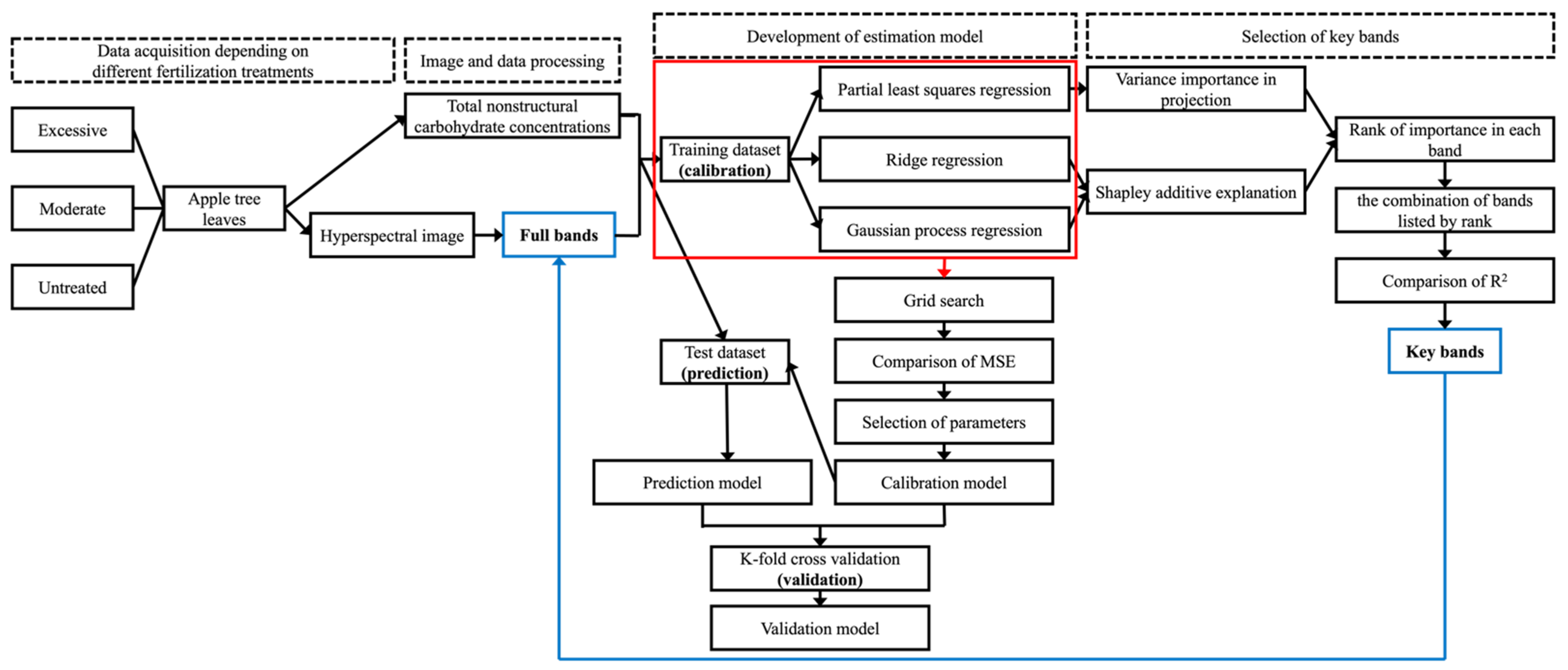
Figure 4.
Reflectance curves of the apple tree canopy area obtained by hyperspectral imaging.
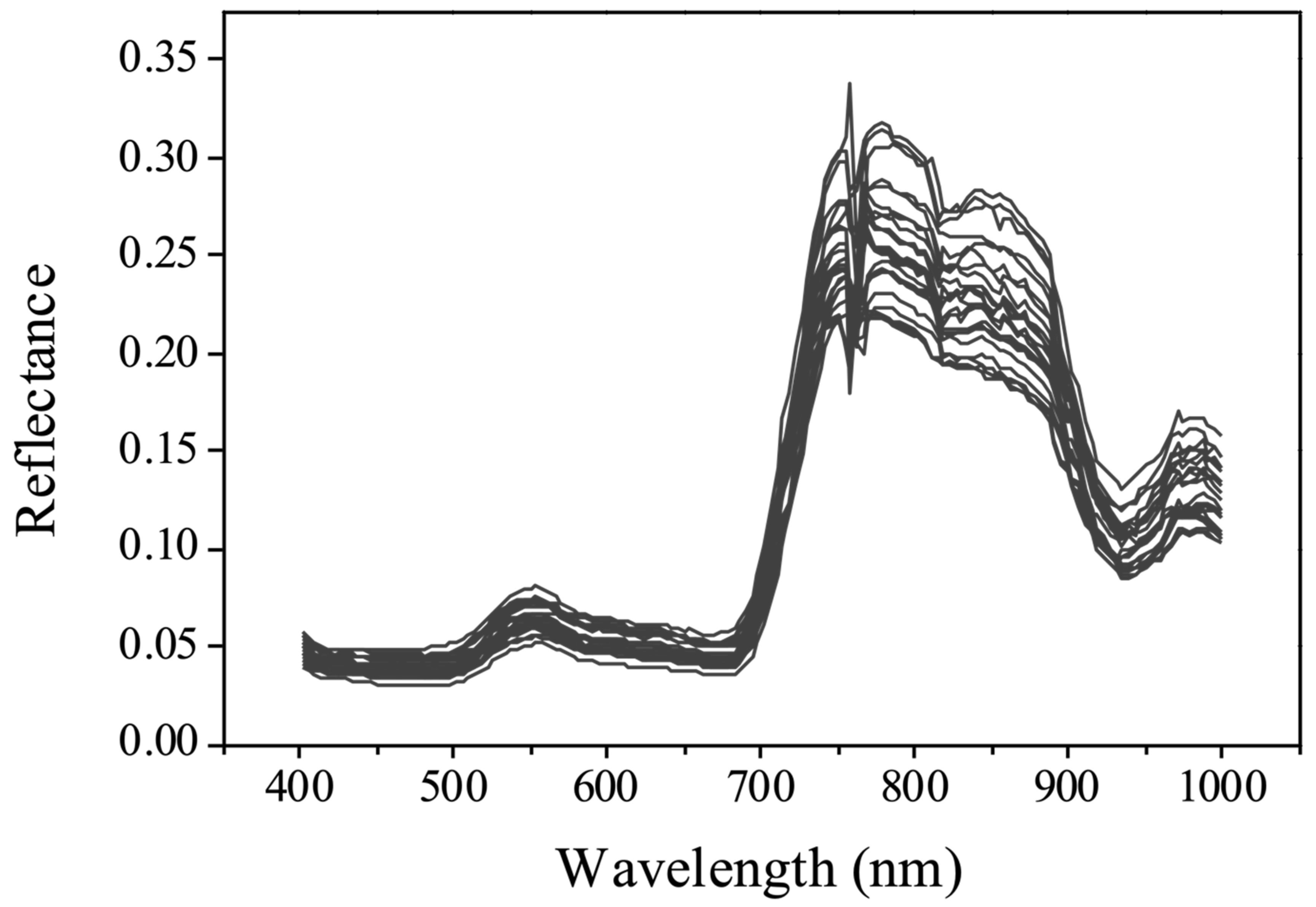
Figure 5.
Linear relationship between the measured TNC concentration and estimation by the GP-based model: (a) training and (b) test datasets with full bands; (c) training and (d) test datasets with key bands.
Figure 5.
Linear relationship between the measured TNC concentration and estimation by the GP-based model: (a) training and (b) test datasets with full bands; (c) training and (d) test datasets with key bands.
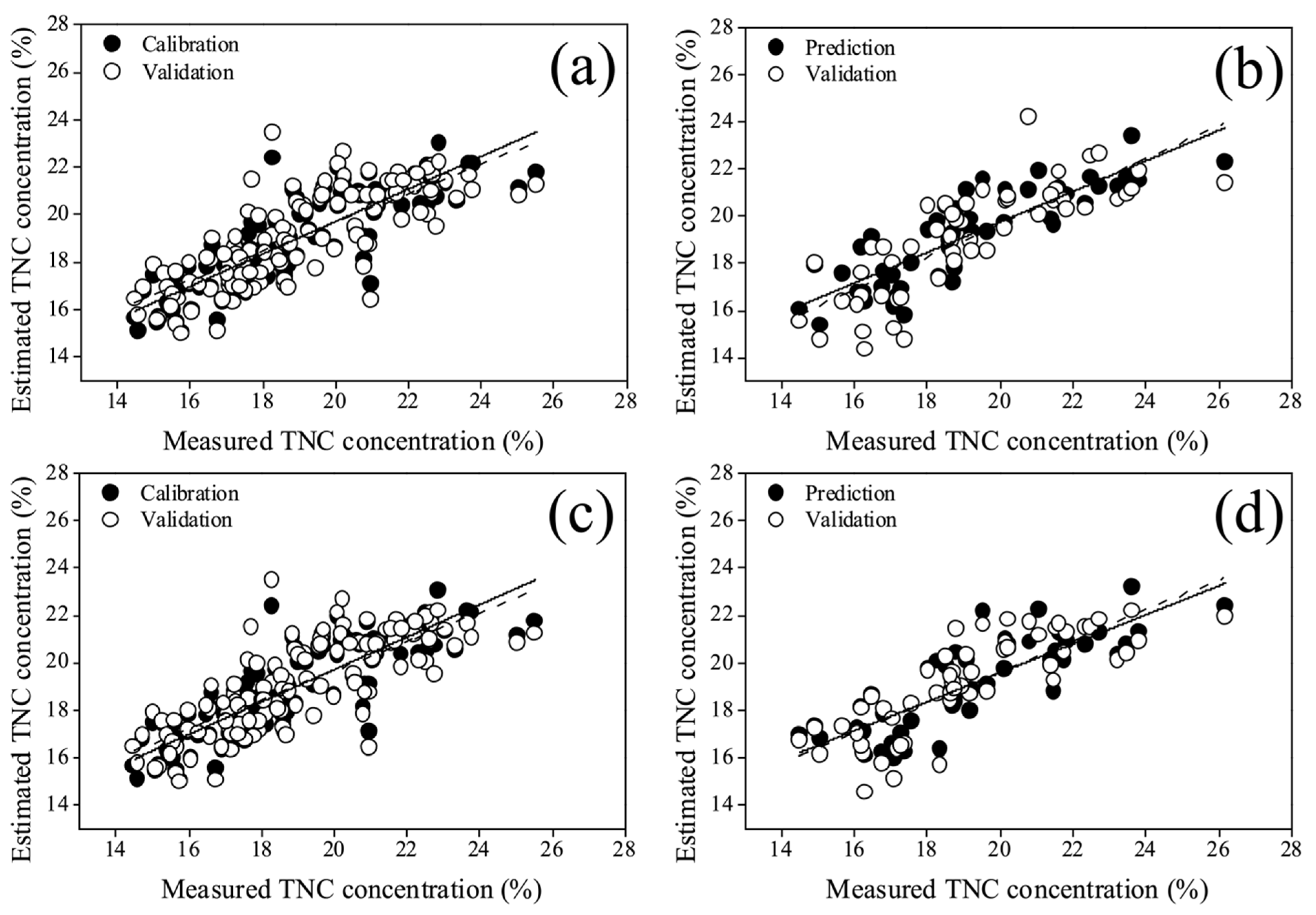
Figure 6.
Shapley additive explanation values depending on the number of key bands used to estimate the TNC concentration: (a) 12, (b) 10, (c) 9, and (d) 6 key bands.
Figure 6.
Shapley additive explanation values depending on the number of key bands used to estimate the TNC concentration: (a) 12, (b) 10, (c) 9, and (d) 6 key bands.
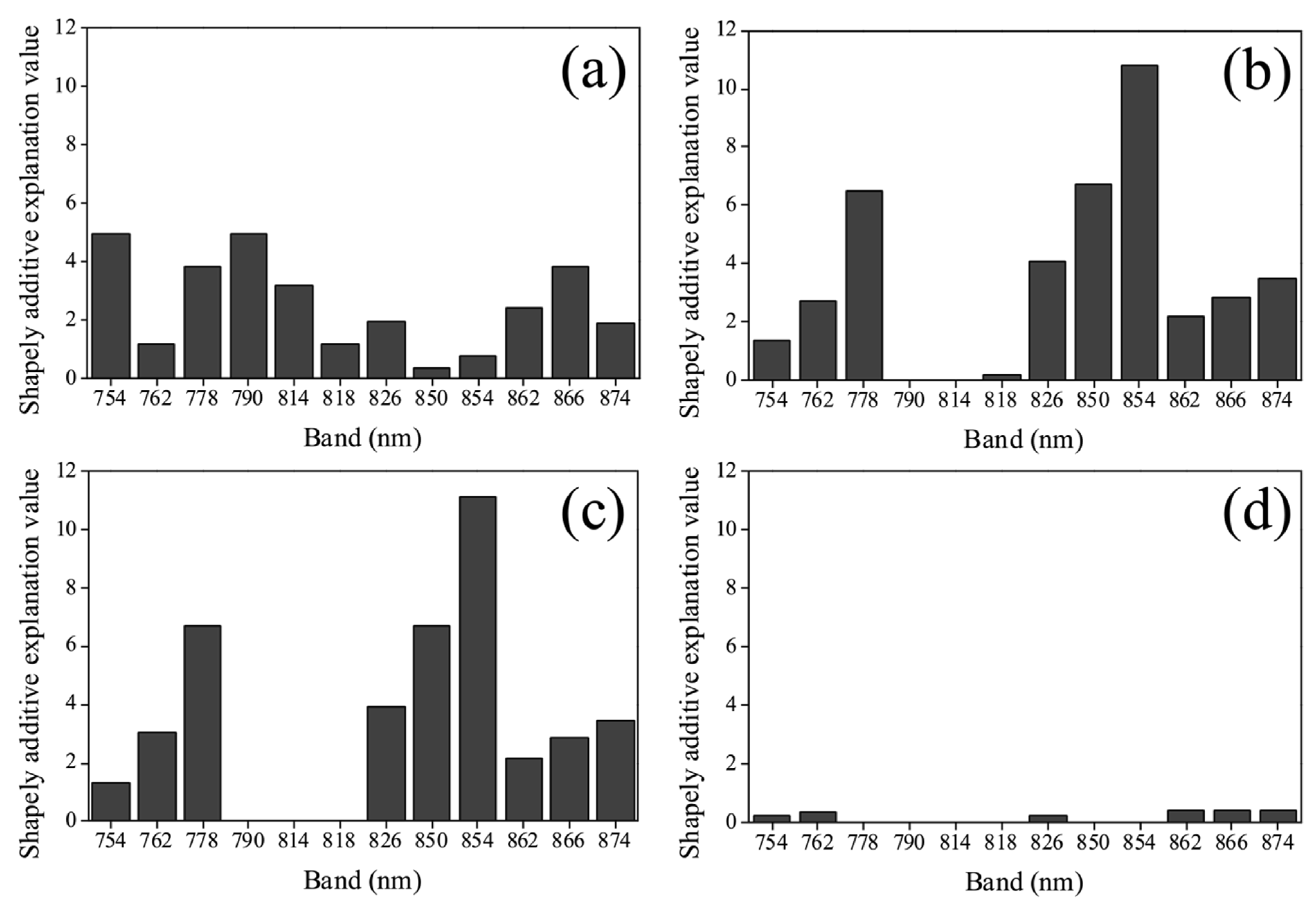
Figure 7.
Maps of the TNC concentration in apple tree leaves estimated by the GP-based model using key bands: (a) May 23; (b) June 17; (c) July 28; (d) September 7.
Figure 7.
Maps of the TNC concentration in apple tree leaves estimated by the GP-based model using key bands: (a) May 23; (b) June 17; (c) July 28; (d) September 7.


Table 1.
Flight and hyperspectral imaging specifications.
| Information | |
|---|---|
| Field coordinates | Coordinate 1: 35.828626, 127.031448 Coordinate 2: 35.828377, 127.031132 Coordinate 3: 35.828085, 127.031484 Coordinate 4: 35.828355, 127.031813 |
| Flight speed | 6 m/s |
| Overlap | 70% |
| Altitude | 60 m |
| Ground sample distance | 4.4 cm/pixel |
Table 2.
Two-sample t-test of the TNC concentration in apple tree leaves depending on the growing season and nitrogen fertilization.
Table 2.
Two-sample t-test of the TNC concentration in apple tree leaves depending on the growing season and nitrogen fertilization.
| May 23 | June 3 | June 17 | July 4 | July 19 | July 28 | August 16 | September 07 | September 21 | |
|---|---|---|---|---|---|---|---|---|---|
| E * | 1.04 a ** | 0.86 a | 1.27 a | 2.28 a | 2.47 a | 1.54 a | 2.29 a | 2.00 a | 1.12 a |
| M | 0.96 a | 1.04 a | 1.10 a | 1.20 a | 0.61 a | 1.44 b | 1.54 a | 1.45 a | 1.48 b |
| U | 1.20 a | 1.79 a | 0.46 a | 1.04 a | 0.62 a | 0.95 b | 1.84 a | 0.75 a | 1.36 b |
| All | 1.04 A | 1.38 BC | 1.05 A | 1.72 C | 1.43 B | 1.65 D | 1.96 EF | 1.45 DE | 1.77 F |
* E: excessive fertilization, M: moderate fertilization, and U: untreated fertilization. ** Two-sample t-test at the significance level (p-value < 0.05) with mean ± standard deviation: uppercase letters indicate significant differences between dates, and lowercase letters indicate significant differences between different nitrogen fertilizations.
Table 3.
Estimation performance of models using full bands.
| PLS | RR | GP | ||
|---|---|---|---|---|
| n * | 127 | |||
| Standard deviation | 2.46 | |||
| (Training) Calibration | R2 | 0.71 | 0.73 | 0.73 |
| RMSE (%) | 1.32 | 1.29 | 1.29 | |
| RE (%) | 6.91 | 6.76 | 6.76 | |
| (Training) Validation | R2 | 0.61 | 0.59 | 0.59 |
| RMSE (%) | 1.54 | 1.57 | 1.57 | |
| RE (%) | 8.07 | 8.22 | 8.22 | |
| n | 55 | |||
| Standard deviation | 2.27 | |||
| (Test) Prediction | R2 | 0.70 | 0.72 | 0.72 |
| RMSEP (%) | 1.41 | 1.37 | 1.37 | |
| RE (%) | 7.43 | 7.22 | 7.22 | |
| (Test) Validation | R2 | 0.57 | 0.64 | 0.64 |
| RMSEP (%) | 1.68 | 1.55 | 1.55 | |
| RE (%) | 8.86 | 8.17 | 8.17 | |
* n: number of samples.
Table 4.
Selected key bands for different models.
| PLS | RR | GP | |
|---|---|---|---|
| Band 1 | 401 | 754 | 754 |
| Band 2 | 405 | 762 | 762 |
| Band 3 | 697 | 778 | 778 |
| Band 4 | 701 | 826 | 826 |
| Band 5 | 705 | 850 | 850 |
| Band 6 | 709 | 854 | 854 |
| Band 7 | 758 | 862 | 862 |
| Band 8 | 762 | 866 | 866 |
| Band 9 | 766 | 874 | 874 |
Table 5.
Estimation performance of models using key bands.
| PLS | RR | GP | ||
|---|---|---|---|---|
| n * | 127 | |||
| Stand ard deviation | 2.46 | |||
| (Training) Calibration | R2 | 0.71 | 0.73 | 0.73 |
| RMSE (%) | 1.32 | 1.29 | 1.29 | |
| RE (%) | 6.91 | 6.76 | 6.76 | |
| (Training) Validation | R2 | 0.61 | 0.59 | 0.59 |
| RMSE (%) | 1.54 | 1.57 | 1.57 | |
| RE (%) | 8.07 | 8.22 | 8.22 | |
| n | 55 | |||
| Standard deviation | 2.27 | |||
| (Test) Prediction | R2 | 0.30 | 0.63 | 0.68 |
| RMSEP (%) | 2.16 | 1.56 | 1.46 | |
| RE (%) | 11.4 | 8.23 | 7.70 | |
| (Test) Validation | R2 | 0.12 | 0.61 | 0.65 |
| RMSEP (%) | 2.41 | 1.62 | 1.52 | |
| RE (%) | 12.7 | 8.54 | 8.01 | |
* n: number of samples.
Table 6.
Coefficient of determination (R2) depending on the number of bands selected for the GP-based model.
Table 6.
Coefficient of determination (R2) depending on the number of bands selected for the GP-based model.
| Number of Bands | Training Dataset | Test Dataset | ||
|---|---|---|---|---|
| 15 | Calibration | 0.73 | Prediction | 0.56 |
| Validation | 0.59 | Validation | 0.55 | |
| 14 | Calibration | 0.73 | Prediction | 0.56 |
| Validation | 0.59 | Validation | 0.56 | |
| 13 | Calibration | 0.73 | Prediction | 0.55 |
| Validation | 0.59 | Validation | 0.56 | |
| 12 | Calibration | 0.73 | Prediction | 0.55 |
| Validation | 0.59 | Validation | 0.55 | |
| 11 | Calibration | 0.73 | Prediction | 0.68 |
| Validation | 0.59 | Validation | 0.64 | |
| 10 | Calibration | 0.73 | Prediction | 0.68 |
| Validation | 0.59 | Validation | 0.63 | |
| 9 | Calibration | 0.73 | Prediction | 0.68 |
| Validation | 0.59 | Validation | 0.65 | |
| 8 | Calibration | 0.73 | Prediction | 0.62 |
| Validation | 0.59 | Validation | 0.58 | |
| 7 | Calibration | 0.73 | Prediction | 0.62 |
| Validation | 0.59 | Validation | 0.58 | |
| 6 | Calibration | 0.73 | Prediction | 0.42 |
| Validation | 0.59 | Validation | 0.45 | |
| 5 | Calibration | 0.73 | Prediction | 0.39 |
| Validation | 0.59 | Validation | 0.57 | |
Disclaimer/Publisher’s Note: The statements, opinions and data contained in all publications are solely those of the individual author(s) and contributor(s) and not of MDPI and/or the editor(s). MDPI and/or the editor(s) disclaim responsibility for any injury to people or property resulting from any ideas, methods, instructions or products referred to in the content. |
© 2023 by the authors. Licensee MDPI, Basel, Switzerland. This article is an open access article distributed under the terms and conditions of the Creative Commons Attribution (CC BY) license (https://creativecommons.org/licenses/by/4.0/).
Share and Cite
MDPI and ACS Style
Kang, Y.-S.; Park, K.-S.; Kim, E.-R.; Jeong, J.-C.; Ryu, C.-S. Estimation of the Total Nonstructural Carbohydrate Concentration in Apple Trees Using Hyperspectral Imaging. Horticulturae 2023, 9, 967. https://doi.org/10.3390/horticulturae9090967
AMA Style
Kang Y-S, Park K-S, Kim E-R, Jeong J-C, Ryu C-S. Estimation of the Total Nonstructural Carbohydrate Concentration in Apple Trees Using Hyperspectral Imaging. Horticulturae. 2023; 9(9):967. https://doi.org/10.3390/horticulturae9090967
Chicago/Turabian StyleKang, Ye-Seong, Ki-Su Park, Eun-Ri Kim, Jong-Chan Jeong, and Chan-Seok Ryu. 2023. "Estimation of the Total Nonstructural Carbohydrate Concentration in Apple Trees Using Hyperspectral Imaging" Horticulturae 9, no. 9: 967. https://doi.org/10.3390/horticulturae9090967
Note that from the first issue of 2016, this journal uses article numbers instead of page numbers. See further details here.