Impact of an Induced Magnetic Field on the Stagnation-Point Flow of a Water-Based Graphene Oxide Nanoparticle over a Movable Surface with Homogeneous–Heterogeneous and Chemical Reactions

Abstract

Water has attracted plenty of attention as a lubricant for manufacturing due to the fact that it is inexpensive, environmentally friendly, and efficient. Because of their outstanding mechanical capabilities, water dispensability, and range of real applications, graphene oxide (GO) materials have the potential to augment the effectiveness of water lubrication. With this encouragement, we inspect the impact of induced magnetism on the fluid flow near a stagnation point dispended with water-based GO nanoparticles caused by a movable surface with a homogeneous–heterogeneous chemical reaction. The leading equations and their related boundary constraints are first transformed into a non-dimensional form through the utilization of the similarity technique. The consequent equations are then numerically solved by employing the bvp4c scheme. Those figures are used to exemplify the stimulation of the relevant constraints on the fluid flow, induced magnetic profiles, temperature profiles, concentration profiles, heat transfer, and friction factor. It is observed that the nanoparticle’s volume fraction enhances the heat transfer rate, as well as the friction factor. The heat transfer and friction factor escalate by almost 11.71% and 0.96% for the respective upper-branch solutions due to the larger impacts of nanoparticles’ volume fractions, while for the lower-branch solutions, they are augmented at about 21.8% and 0.66%, respectively. In addition, double solutions can be found in the limited values of a movable parameter.

1. Introduction

Currently, the heat transfer of fluid flow contributes significantly to its utilization in the coating of wire, paper production, the process of heat exchangers, cooling process, etc. The high thermal conductivity of nanoparticles dispersed in regular fluids at a nanoscale, referred to as nanofluids, enhances the thermal conductivity of the regular liquids. Choi and Eastman [1] examined the heat transport of nanofluids initially. Later on, this work was extended by Khan and Pop [2] by considering nanofluid flow through a stretchable sheet. Bachok et al. [3] studied the unsteady flow induced by a nanofluid via a movable surface and presented dual solutions. The effects of colloidal particles on the flow and heat transfer of nanofluids submerged in a porous media from a stretchable sheet were examined numerically by Gireesha et al. [4]. Jain et al. [5] employed rainbow schlieren deflectometry to inspect a water-based Al₂O₃ nanofluid. They discovered that as the nanofluid value fraction uplifted, the thermal boundary layer width decreased. Rao et al. [6] examined the water-based Al₂O₃ nanofluid inside a cavity with free convection. According to the authors, the use of a large concentration of nanofluid resulted in larger convective loops, which improved the mixing of the nanofluid and heat transfer. Makinde and Mishra [7] examined the unchangeable viscosity induced by nanofluid near a stagnation point through a heated stretching sheet with a radiation effect. The unsteady 3D flow of a nanofluid past a stretchable penetrable cylinder with chemical reaction was inspected by Bhatti et al. [8]. Zuhra et al. [9] utilized a water-based fluid with graphene nanoparticles to inspect the properties of heat transfer of non-Newtonian liquids from a stretchable sheet. Khan et al. [10] scrutinized the 2D MHD flow of Sisko nanoliquid caused by a stretchable/shrinkable sheet with zero mass flux and presented dual solutions. The influence of an irregular radiation effect on the non-Newtonian nanofluid via a shrinkable surface was inspected by Zaib et al. [11]. Nayak and Mishra [12] analyzed the squeezing flow submerged by nanofluid through a couple of parallel plates. Recently, Waini et al. [13] theoretically inspected the impact of a magnetic field on the nanofluid flow by employing the Tiwari–Das model through a shrinking cylinder, and found double solutions.

The induced magnetization plays an important part in different procedures such as nuclear reactors, astronautical re-entry, thermo-magneto aerodynamics, and magneto energy generator systems. When the magnetic Reynolds number is pretty high, the induced magnetism must be taken into account. Glauert [14] inspected the impression of an induced magnetic field (IMF) on the flow caused by a magnetized plate with a uniform magnetic effect. He provided a series solution for the magnetic and flow fields. The aligned magnetic impact on transient flow approaching a semi-infinite plate was carefully examined by Takhar et al. [15]. In addition to the mechanisms of heat and mass transfer, Alom et al. [16] took into account the influence of induced magnetism through a vertical plate with mixed convection filled with a permeable matrix. They also featured steady fluxes of mass and heat at the corresponding wall boundary. Then, Ahmed and Chamkha [17] investigated the forced convective flow past a penetrable vertical plate affected by an induced magnetism. By using the series-expansion technique, they also carefully looked into the impact of chemical reactions, heat source/sink, and thermal radiation. Bég et al. [18] scrutinized the impression of an aligned magnetic field on the mixed convective flow through a non-conducting and translating plate. They provided the numerical results for a wide variety of magneto Prandtl and Hartmann numbers. Ghosh et al. [19] discovered accurate solutions for a natural convective magneto flow caused by an infinite vertical plate with IMF. The consequences of an induced magnetism impact via a stagnation-point flow toward a stretching sheet were inspected by Ali et al. [20]. Gireesha et al. [21] investigated how heat transfer and melting were impacted by generated magnetism in a nanofluid flow. Sheikholeslami and Rokni [22] investigated the impact of induced magnetism incorporating a two-phase nanofluid. They concluded that the temperature gradient increased by increasing the suction parameter, but decreased by increasing the thermophoretic parameter. Recently, Hou et al. [23] analyzed the induced magnetism with entropy generation on the stagnation-point flow of a pseudoplastic fluid filled with nanofluid past a deformable surface.

Both heterogeneous and homogeneous reactions occur in numerous chemically reactive systems, including catalysis, combustion, and biological structures. The interactions amid the homogeneous reactions taking place in the bulk of the liquid and the heterogeneous reactions on certain catalyst interfaces are typically very complicated. These interactions involve the utilization and production of responding species at various rates within the liquid and on the catalyst interface as well as further comments on these rates of reaction through temperature changes in the reacting liquid, which then change the motion of the fluid. As a result, the fluid, reactant species concentrations, and temperatures of the fluid/surface are all coupled in three ways. There may be a noticeable response both inside the homogeneous or bulk reactions and on the catalytic interface in certain catalytic-driven reactions that are significant in the chemical industries. The research on propane and ammonia/methane oxidations on platinum was explored by Williams et al. [24,25], and Song et al. [26] provided examples of such homogeneous–heterogeneous processes. These phenomena are represented by a boundary-layer flow, normally a stagnation-point flow [27,28,29] in which exothermic reactions are permitted both on the catalyst’s surface and inside of the boundary-layer flow. Chaudhary and Merkin [30,31] took into consideration a straightforward form for heterogeneous–homogeneous reactions in fluid flow, where the bulk-type reaction is supposed to be specified through isothermal cubic autocatalator kinetics and the surface heterogeneous reaction by first-order kinetics. Bachok et al. [32] investigated the impact of a homogeneous–heterogeneous reaction on a stagnation-point flow from a stretching surface and presented non-unique solutions. Ibrahim [33] inspected the induced magnetism near a stagnation point incorporated by Maxwell nanofluid across a heated stretching sheet. More about the significance of the induced magnetic effect was observed in refs. [34,35,36,37].

As observed above, the characteristics of heat-transport fluid flow involving nanoparticles are explored in the present literature. Additionally, research on heat-transfer flows including nanoparticles has shown a crucial role for these flows in the thermal improvement of various industrial systems, including solar-powered electronics, air conditioning, and other technical and natural processes. Keeping this in mind, the present work aspires to inspect the impact of induced magnetism on the characteristics of heat-transfer fluid flow incorporated by water-based graphene oxide nanoparticles caused by a movable surface with heterogeneous–homogeneous chemical reactions. The physical effects of the significant parameters are discussed in depth through the use of graphical and tabular forms.

2. Problem Formulation

Consider a two-dimensional (2D) steady flow near a stagnation point incorporating nanofluid from a movable sheet with induced magnetism and homogeneous–heterogeneous chemical reactions (see Figure 1), where $(\overline{x},\overline{y})$ are the Cartesian coordinates along the $\overline{x}-$axis calculated along the sheet and the $\overline{y}-$axis is normal to it whilst the corresponding flow is at $\overline{y}\ge 0$. It is supposed that the movable sheet velocity is ${\overline{u}}_w\left(\overline{x}\right)$ and that the velocity of the far (inviscid) flow is ${\overline{u}}_e\left(\overline{x}\right)$. Additionally, it is assumed that the sheet’s temperature is ${\overline{T}}_w$, while the far flow temperature is ${\overline{T}}_{\infty }$. The sheet is non-conducting, and a uniformly strong magnetic field $H_0$ is injected. Moreover, the induced magnetism is considered to be provided along the $\overline{y}-$direction and the parallel component ${\overline{H}}_1$ gets closer to the value ${\overline{H}}_e\left(\overline{x}\right)=H_e{H}_0$ in the flow of free-stream and the normal component of the induced magnetism ${\overline{H}}_2$ vanishes near the wall surface of the sheet. Following Merkin [38], the chemical reaction is given by:

$$A+2B\to 3B\hspace{0.17em}\hspace{0.17em}\hspace{0.17em}\hspace{0.17em}\hspace{0.17em}\hspace{0.17em}\hspace{0.17em}\hspace{0.17em}\hspace{0.17em}\hspace{0.17em}\hspace{0.17em}rate\hspace{0.17em}\left({\epsilon }_c\overline{a}{\overline{b}}^2\right)$$

and it is assumed that the first-order step is the straight-forward heterogeneous reaction:

$$A\to B\hspace{0.17em}\hspace{0.17em}\hspace{0.17em}\hspace{0.17em}\hspace{0.17em}\hspace{0.17em}\hspace{0.17em}\hspace{0.17em}\hspace{0.17em}\hspace{0.17em}\hspace{0.17em}rate\hspace{0.17em}\left({\epsilon }_s\overline{a}\right).$$

Now, $\overline{a}$ and $\overline{b}$ are the species of the concentrations $A$ and $B$, respectively, whilst ${\epsilon }_i\left(c,s\right)$ are the constants rate, where there is a homogeneous concentration $a_0$ of reactant $A$ and in which there is no autocatalyst $B$ past a smooth surface. We also suppose that both reaction processes are isothermal. The nanofluid is made up of water and nanoparticles, namely, graphene oxide (GO). Furthermore, it is assumed that the dispersed nanoparticles have a homogeneous shape and size and are in a condition of thermal equilibrium with the working fluids. The appropriate governing equations are the mass conservation, the momentum, the induced magnetic field, the energy, and the chemical reaction equations, which can be expressed in the respective Cartesian coordinate $(\overline{x},\overline{y})$ as in [31,32,33]:

$$\frac{\partial \overline{u}}{\partial \overline{x}}+\frac{\partial \overline{v}}{\partial \overline{y}}=0$$

(1)

$$\frac{\partial {\overline{H}}_1}{\partial \overline{x}}+\frac{\partial {\overline{H}}_2}{\partial \overline{y}}=0$$

(2)

$$\overline{u}\frac{\partial \overline{u}}{\partial \overline{x}}+\overline{v}\frac{\partial \overline{u}}{\partial \overline{y}}-{\overline{u}}_e\frac{d{\overline{u}}_e}{d\overline{x}}=\frac{{\mu }_{nf}}{{\rho }_{nf}}\frac{{\partial }^2\overline{u}}{\partial {\overline{y}}^2}+\frac{{\mu }_0}{4\pi {\rho }_{nf}}\left({\overline{H}}_1\frac{\partial {\overline{H}}_1}{\partial \overline{x}}+{\overline{H}}_2\frac{\partial {\overline{H}}_1}{\partial \overline{y}}-{\overline{H}}_e\frac{\partial {\overline{H}}_e}{\partial \overline{x}}\right)$$

(3)

$$\overline{u}\frac{\partial {\overline{H}}_1}{\partial \overline{x}}+\overline{v}\frac{\partial {\overline{H}}_1}{\partial \overline{y}}={\overline{H}}_1\frac{\partial \overline{u}}{\partial \overline{x}}+{\overline{H}}_2\frac{\partial \overline{u}}{\partial \overline{y}}+{\mu }_e\frac{{\partial }^2{\overline{H}}_1}{\partial {\overline{y}}^2}$$

(4)

$$\overline{u}\frac{\partial \overline{T}}{\partial \overline{x}}+\overline{v}\frac{\partial \overline{T}}{\partial \overline{y}}=\frac{k_{nf}}{{\left(\rho c_p\right)}_{nf}}\frac{{\partial }^2\overline{T}}{\partial {\overline{y}}^2}$$

(5)

$$\overline{u}\frac{\partial \overline{a}}{\partial \overline{x}}+\overline{v}\frac{\partial \overline{a}}{\partial \overline{y}}=D_A\frac{{\partial }^2\overline{a}}{\partial {\overline{y}}^2}-{\epsilon }_c\overline{a}{\overline{b}}^2$$

(6)

$$\overline{u}\frac{\partial \overline{b}}{\partial \overline{x}}+\overline{v}\frac{\partial \overline{b}}{\partial \overline{y}}=D_A\frac{{\partial }^2\overline{b}}{\partial {\overline{y}}^2}+{\epsilon }_c\overline{a}{\overline{b}}^2$$

(7)

along with the boundary conditions (BCs)

$$\left\{\begin{array}{l}\hspace{0.17em}\overline{u}={\epsilon }_a{\overline{u}}_w\left(\overline{x}\right),\overline{v}=0,{\overline{H}}_1=0,{\overline{H}}_2=0\hspace{0.17em},\overline{T}={\overline{T}}_w,D_A\frac{\partial \overline{a}}{\partial \overline{y}}={\epsilon }_s\overline{a},\hspace{0.17em}{D}_B\frac{\partial \overline{b}}{\partial \overline{y}}=-{\epsilon }_s\overline{a}\hspace{0.17em}\hspace{0.17em}\hspace{0.17em}\mathrm{at}\hspace{0.17em}\hspace{0.33em}\overline{y}=0,\hspace{0.17em}\\ \hspace{0.17em}\overline{u}\to {\overline{u}}_e\left(\overline{x}\right),{\overline{H}}_1\to {\overline{H}}_e\left(\overline{x}\right),\overline{T}\to {\overline{T}}_{\infty },\hspace{0.17em}\overline{a}\to a_0,\hspace{0.17em}\overline{b}\to 0 \hspace{0.33em}\mathrm{as} \overline{y}\to \infty .\end{array}\right.$$

(8)

Here, $\overline{u}$, $\overline{v}$, ${\overline{H}}_1$, and ${\overline{H}}_2$ signify the components of velocity and magnetic vectors along the specified $\overline{x}$ and $\overline{y}$ axes, respectively, while $\overline{T}$ is the requisite posited temperature of the well-known decided nanofluid. In addition, ${\overline{H}}_e\left(\overline{x}\right)$ is the respective $\overline{x}-$magnetic field at the edge of the boundary layer and $D_A$ and $D_B$ are the specified coefficients of diffusion for species $A$ and $B$, respectively. Additionally, the rest of the comprised symbols in the above-stated equations are noted as the thermal conductivity $k_{nf}$, the density ${\rho }_{nf}$, the heat capacity ${\left(\rho c_p\right)}_{nf}$, and the viscosity ${\mu }_{nf}$ of the (GO/water) nanofluid, which are listed as (see Ho et al. [39]):

$$\left.\begin{array}{l}\frac{{\mu }_{nf}}{{\mu }_f}=1+4.93\phi +222.4{\phi }^2,\hspace{0.17em}\hspace{0.17em}\hspace{0.17em}{\left(\rho c_p\right)}_{nf}={\left(\rho c_p\right)}_f\left(1-\phi \right)+\phi {\left(\rho c_p\right)}_{pa}\\ \frac{k_{nf}}{k_f}=1+2.944\phi +19.672{\phi }^2,\hspace{0.17em}\hspace{0.17em}{\rho }_{nf}={\rho }_f\left(1-\phi \right)+\phi {\rho }_{pa}.\end{array}\right\}$$

(9)

In the above correlations, $\phi$ denotes the nanoparticles volume fraction, while $\phi =0$ resembles the common (working)-based fluid. Likewise, the subscript indexes $f,nf$ and $pa$ demonstrate the common-based fluids, nanoliquids, and solid nanoparticles, respectively. The GO nanoparticles and the base fluid physical data are displayed in

Table 1. Thermophysical data of the base fluid and GO nanoparticles [40].

Physical Properties	Water	GO
$k\left(W/mK\right)$	0.613	5000
$c_p\left(J/kgK\right)$	4179	717
$\rho \left(kg/m^3\right)$	997.1	1800

.

The subsequent necessary hypothesized non-dimensional quantities are supplied to demonstrate the given problem in the dimensionless form:

$$\left\{\begin{array}{l}{x}_a=\frac{\overline{x}}{l_a},y_a=\frac{\overline{y}}{l_a}{\mathrm{Re}}^{\frac{1}{2}},u_a=\frac{\overline{u}}{U_0},v_a=\frac{\overline{v}}{U_0}{\mathrm{Re}}^{\frac{1}{2}},H_{1a}=\frac{{\overline{H}}_1}{H_0},H_{2a}=\frac{{\overline{H}}_2}{H_0}{\mathrm{Re}}^{\frac{1}{2}},\mathrm{Re}=\frac{U_0{l}_a}{{\upsilon }_f},\\ u_{ea}=\frac{{\overline{u}}_e}{U_0},u_{wa}=\frac{{\overline{u}}_w}{U_0},H_{ea}=\frac{{\overline{H}}_e}{H_0},\overline{T}-{\overline{T}}_{\infty }=T_a\mathrm{\Delta }\overline{T},a_a=\frac{\overline{a}}{a_0},b_a=\frac{\overline{b}}{a_0}\end{array}\right.$$

(10)

where ${\epsilon }_c=U_0/l_a{a}_0^2$, $l_a{U}_0={\upsilon }_f$, and $\mathrm{\Delta }\overline{T}={\overline{T}}_w-{\overline{T}}_{\infty }$. Here, $l_a$ is the characteristic length of the sheet, which is the square root of the area of the sheet. This quantity is required for the constructing of the dimensionless quantities. Further, utilizing Equation (10) in Equations (1)–(7) along with BCs (8) yields:

$$\frac{\partial u_a}{\partial x_a}+\frac{\partial v_a}{\partial y_a}=0$$

(11)

$$\frac{\partial H_{1a}}{\partial x_a}+\frac{\partial H_{2a}}{\partial y_a}=0$$

(12)

$$u_a\frac{\partial u_a}{\partial x_a}+v_a\frac{\partial u_a}{\partial y_a}-u_{ea}\frac{d{u}_{ea}}{d{x}_a}=\frac{{\mu }_{nf}/{\mu }_f}{{\rho }_{nf}/{\rho }_f}\frac{{\partial }^2{u}_a}{\partial y_a^2}+\frac{{\mathrm{\Sigma }}_a}{{\rho }_{nf}/{\rho }_f}\left(\begin{array}{l}{H}_{1a}\frac{\partial H_{1a}}{\partial x_a}+H_{2a}\frac{\partial H_{1a}}{\partial y_a}\\ -H_{ea}\frac{\partial H_{ea}}{\partial x_a}\end{array}\right)$$

(13)

$$u_a\frac{\partial H_{1a}}{\partial x_a}+v_a\frac{\partial H_{1a}}{\partial y_a}=H_{1a}\frac{\partial u_a}{\partial x_a}+H_{2a}\frac{\partial u_a}{\partial y_a}+\frac{1}{{\mathrm{Pr}}_a}\frac{{\partial }^2{H}_{1a}}{\partial y_a^2}$$

(14)

$$u_a\frac{\partial T_a}{\partial x_a}+v_a\frac{\partial T_a}{\partial y_a}=\frac{1}{\mathrm{Pr}}\frac{k_{nf}/k_f}{{\left(\rho c_p\right)}_{nf}/{\left(\rho c_p\right)}_f}\frac{{\partial }^2{T}_a}{\partial y_a^2}$$

(15)

$$u_a\frac{\partial a_a}{\partial x_a}+v_a\frac{\partial a_a}{\partial y_a}=\frac{1}{S{c}_a}\frac{{\partial }^2{a}_a}{\partial y_a}-a_a{b}_a^2$$

(16)

$$u_a\frac{\partial b_a}{\partial x_a}+v_a\frac{\partial b_a}{\partial y_a}=\frac{{\delta }_a}{S{c}_a}\frac{{\partial }^2{b}_a}{\partial y_a}+a_a{b}_a^2$$

(17)

which have to be solved along with the boundary conditions (BCs):

$$\left\{\begin{array}{l}\hspace{0.17em}{u}_a={\epsilon }_a{u}_{wa}\left(x_a\right),v_a=0,H_{1a}=0,H_{2a}=0\hspace{0.17em},T_a=1,\frac{\partial a_a}{\partial y_a}={\gamma }_s{a}_a,\hspace{0.17em}{\delta }_a\frac{\partial b_a}{\partial y_a}=-{\gamma }_s{a}_a\hspace{0.17em}\hspace{0.17em}\hspace{0.17em}\mathrm{at}\hspace{0.17em}\hspace{0.33em}{y}_a=0,\\ \hspace{0.17em}{u}_a\to u_{ea}\left(x_a\right),H_{1a}\to H_{ea}\left(x_a\right),T_a\to 0,\hspace{0.17em}{a}_a\to 1,\hspace{0.17em}{b}_a\to 0 \hspace{0.33em}\mathrm{as} y_a\to \infty .\end{array}\right.$$

(18)

In the above set of dimensionless Equations (11)–(18), the following distinguished parameters are included such as the reciprocal magnetic (PN) factor ${\mathrm{Pr}}_a$, the magnetic factor ${\mathrm{\Sigma }}_a$, the PN (Prandtl number) $\mathrm{Pr}$, the Schmidt number $S{c}_a$, the ratio of the diffusion coefficients ${\delta }_a$, and the dimensionless measure of the heterogeneous reaction ${\gamma }_s$, which are mathematically expressed as

$${\mathrm{\Sigma }}_a=\frac{{\mu }_0{H}_0^2}{4\pi U_0^2},{\mathrm{Pr}}_a=\frac{{\upsilon }_f}{{\mu }_e},\mathrm{Pr}=\frac{{\upsilon }_f}{{\alpha }_f},S{c}_a=\frac{{\upsilon }_f}{D_A},{\delta }_a=\frac{D_B}{D_A},{\gamma }_s=\frac{{\epsilon }_s}{D_A}\sqrt{\frac{{\upsilon }_f}{{\epsilon }_c{a}_0^2}}$$

(19)

where ${\upsilon }_f$ signposts the kinematic viscosity and ${\alpha }_f$ designates the thermal diffusivity of the normal base fluid. Although we could anticipate that the chemical reactants species $A$ and $B$ would be comparable in size, in general, their diffusion coefficients would not be equal. In the special case where $D_A=D_B$ (i.e., ${\delta }_a=1$), Equations (16) and (17) can be combined to give:

$$a_a\left(x_a,y_a\right)+b_a\left(x_a,y_a\right)=1$$

(20)

so that Equation (16) becomes

$$u_a\frac{\partial a_a}{\partial x_a}+v_a\frac{\partial a_a}{\partial y_a}=\frac{1}{S{c}_a}\frac{{\partial }^2{a}_a}{\partial y_a}-a_a{\left(1-a_a\right)}^2$$

(21)

In order to introduce the self-similarity transformations, the following equation is employed:

$$\left\{\begin{array}{l}{u}_a=x_{a}F\prime \left(\xi \right),\hspace{0.17em}{v}_a=-F\left(\xi \right),\hspace{0.17em}{H}_{1a}=x_{a}G\prime \left(\xi \right),\hspace{0.17em}{H}_{2a}=-G\left(\xi \right),\\ T_a=\theta \left(\xi \right),\hspace{0.17em}\hspace{0.17em}{a}_a=S\left(\xi \right),\hspace{0.17em}\hspace{0.17em}\xi =y_a,\end{array}\right.$$

(22)

where primes indicate differentiation with respect to $\xi$. Moreover, the following equation is obtained:

$$u_{wa}\left(x_a\right)=x_a,\hspace{0.17em}\hspace{0.17em}{u}_{ea}\left(x_a\right)=x_a,H_{ea}\left(x_a\right)=x_a.$$

(23)

Substituting variables (22) and (23) into the dimensionless equations, the continuity Equations (11) and (12) are identically satisfied, while the rest of Equations (13)–(15), (18), and (21) yield the following nonlinear ordinary (similarity) differential equations for the flow, induced magnetic field, heat transfer, and chemical reaction:

$$\frac{{\mu }_{nf}/{\mu }_f}{{\rho }_{nf}/{\rho }_f}F‴+FF″-F{\prime }^2+1+\frac{{\mathrm{\Sigma }}_a}{{\rho }_{nf}/{\rho }_f}\left(G{\prime }^2-GG″-1\right)=0$$

(24)

$$\frac{G‴}{{\mathrm{Pr}}_a}+FG″-GF″=0$$

(25)

$$\frac{1}{\mathrm{Pr}}\frac{k_{nf}/k_f}{{\left(\rho c_p\right)}_{nf}/{\left(\rho c_p\right)}_f}\theta ″+F\theta \prime =0$$

(26)

$$\frac{S″}{S{c}_a}+FS\prime -S{\left(1-S\right)}^2=0$$

(27)

which are solved along with the BCs:

$$\left\{\begin{array}{l}\hspace{0.17em}F\prime \left(\xi \right)={\epsilon }_a,F\left(\xi \right)=0,G\prime \left(\xi \right)=0,G\left(\xi \right)=0\hspace{0.17em},S\prime \left(\xi \right)={\gamma }_{s}S,\theta \left(\xi \right)=1,\hspace{0.17em}\hspace{0.17em}\hspace{0.17em}\mathrm{at}\hspace{0.17em}\hspace{0.33em}\xi =0,\hspace{0.17em}\\ \hspace{0.17em}F\prime \left(\xi \right)\to 1,G\prime \left(\xi \right)\to 1,\theta \left(\xi \right)\to 0,\hspace{0.17em}S\left(\xi \right)\to 1, \hspace{0.33em}\mathrm{as} \xi \to \infty .\end{array}\right.$$

(28)

The stretching sheet is denoted by ${\epsilon }_a>0$, the shrinking sheet is denoted by ${\epsilon }_a<0$, and the static sheet is denoted by ${\epsilon }_a=0$.

The physical engineering quantities of interest are the skin friction coefficient $C_f$ and the local Nusselt number $N{u}_{\overline{x}}$, which are given by

$$C_f=\frac{{\mu }_{nf}}{{\rho }_f{\overline{u}}_w^2\left(\overline{x}\right)}\hspace{0.17em}{\left.\left(\frac{\partial \overline{u}}{\partial \overline{y}}\right)\right|}_{\overline{y}=0},$$

(29)

and

$$N{u}_{\overline{x}}=\frac{\overline{x}}{k_f\mathrm{\Delta }\overline{T}}\left({\left.-k_{nf}\left(\frac{\partial \overline{T}}{\partial \overline{y}}\right)\right|}_{\overline{y}=0}\right)$$

(30)

Utilizing Equation (10) in the above Equations (29) and (30), we get

$$C_f=\frac{{\mu }_{nf}/{\mu }_f}{{\mathrm{Re}}^{\frac{1}{2}}{u}_{wa}^2\left(x_a\right)}\hspace{0.17em}{\left.\left(\frac{\partial u_a}{\partial y_a}\right)\right|}_{y_a=0},$$

(31)

and

$$N{u}_{x_a}=-\frac{k_{nf}}{k_f}{x}_a{\mathrm{Re}}^{\frac{1}{2}}{\left.\left(\frac{\partial T_a}{\partial y_a}\right)\right|}_{y_a=0}$$

(32)

Further, substituting Equations (22) and (23) into the above dimensionless Equations (31) and (32) yield

$$x_a{\mathrm{Re}}^{\frac{1}{2}}{C}_f=\frac{\hspace{0.17em}{\mu }_{nf}}{{\mu }_f}F″\left(0\right),$$

(33)

and

$$\frac{N{u}_{x_a}}{x_a{\mathrm{Re}}^{\frac{1}{2}}}=-\frac{k_{nf}}{k_f}\theta \prime \left(0\right)$$

(34)

Hence, $x_a=\frac{\overline{x}}{l_a}$ and $\mathrm{Re}=\frac{U_0{l}_a}{{\upsilon }_f}$ are the dimensionless x-axis coordinates and the Reynolds number, respectively.

3. Numerical Procedure

This section exhibits the problem-solving approaches, as well as the implications of the numerical scheme under consideration. From the necessary governing equations, the attached non-linear similarity Equations (24)–(27) with BCs (28) are transfigured. These equations are extremely complicated, highly nonlinear, and not an easy task to solve analytically. Therefore, the acquired similarity equations were solved numerically by the boundary-value problem of fourth-order (bvp4c) package in the MATLAB software. In addition, the three-stage Lobatto IIIA formula was further achieved using a built-in category solver in the MATLAB program that uses the finite-difference method. The details of the approach under consideration are provided in [41,42]. Using the novel (mathematical notation) parameters, the second- and third-order ODEs were converted to their equivalent first-order dimensionless equations (ODEs) in the documented literature that follows. Let the parameters be as follows to continue the scheme’s current procedure:

$$F={\mathrm{\Sigma }}_1,F\prime ={\mathrm{\Sigma }}_2,F″={\mathrm{\Sigma }}_3,G={\mathrm{\Sigma }}_4,G\prime ={\mathrm{\Sigma }}_5,G″={\mathrm{\Sigma }}_6,\theta ={\mathrm{\Sigma }}_7,\theta \prime ={\mathrm{\Sigma }}_8,S={\mathrm{\Sigma }}_9,S\prime ={\mathrm{\Sigma }}_{10}$$

(35)

The set of first-order ODEs is obtained by replacing the above new additional parameters in Equations (24)–(27), along with the BCs (28). Hence, one obtains the form:

$$\frac{d}{d\xi }\left(\begin{array}{l}{\mathrm{\Sigma }}_1\\ {\mathrm{\Sigma }}_2\\ {\mathrm{\Sigma }}_3\\ {\mathrm{\Sigma }}_4\\ {\mathrm{\Sigma }}_5\\ {\mathrm{\Sigma }}_6\\ {\mathrm{\Sigma }}_7\\ {\mathrm{\Sigma }}_8\\ {\mathrm{\Sigma }}_9\\ {\mathrm{\Sigma }}_{10}\end{array}\right)=\left(\begin{array}{l}{\mathrm{\Sigma }}_2\\ {\mathrm{\Sigma }}_3\\ \frac{{\rho }_{nf}/{\rho }_f}{{\mu }_{nf}/{\mu }_f}\left({\mathrm{\Sigma }}_2^2-{\mathrm{\Sigma }}_1{\mathrm{\Sigma }}_3-1-\frac{{\mathrm{\Sigma }}_a}{{\rho }_{nf}/{\rho }_f}\left({\mathrm{\Sigma }}_5^2-{\mathrm{\Sigma }}_4{\mathrm{\Sigma }}_6-1\right)\right)\\ {\mathrm{\Sigma }}_5\\ {\mathrm{\Sigma }}_6\\ {\mathrm{Pr}}_a\left({\mathrm{\Sigma }}_4{\mathrm{\Sigma }}_3-{\mathrm{\Sigma }}_1{\mathrm{\Sigma }}_6\right)\\ {\mathrm{\Sigma }}_8\\ -\frac{\mathrm{Pr}{\left(\rho c_p\right)}_{nf}/{\left(\rho c_p\right)}_f}{k_{nf}/k_f}{\mathrm{\Sigma }}_1{\mathrm{\Sigma }}_8\\ {\mathrm{\Sigma }}_{10}\\ S{c}_a\left({\mathrm{\Sigma }}_9{\left(1-{\mathrm{\Sigma }}_9\right)}^2-{\mathrm{\Sigma }}_1{\mathrm{\Sigma }}_{10}\right)\end{array}\right)$$

(36)

The subsequent identified and unidentified initial conditions (ICs) are taken into account when handling the set of first-order Equation (36) as an initial value problem (IVP):

$$\left\{\begin{array}{l}{\mathrm{\Sigma }}_1\left(0\right)=0,{\mathrm{\Sigma }}_2\left(0\right)={\epsilon }_a,{\mathrm{\Sigma }}_3\left(0\right)=d_1,\hspace{0.17em}{\mathrm{\Sigma }}_4\left(0\right)=0,{\mathrm{\Sigma }}_5\left(0\right)=0,\hspace{0.17em}\\ {\mathrm{\Sigma }}_6\left(0\right)=d_2,{\mathrm{\Sigma }}_7\left(0\right)=1,{\mathrm{\Sigma }}_8\left(0\right)=d_3,\hspace{0.17em}{\mathrm{\Sigma }}_9\left(0\right)=\frac{1}{{\gamma }_s}{d}_4,{\mathrm{\Sigma }}_{10}\left(0\right)=d_4.\end{array}\right.$$

(37)

Additionally, during the numerical simulations of the bvp4c scheme, the unknown constants $d_1$, $d_2$, $d_3$, and $d_4$ are determined by using the relevant shooting method in the form of a specific approach that the iteration method is continued until the resulting BCs are satisfied:

$${\mathrm{\Sigma }}_2\left(\xi \right)\to 1,{\mathrm{\Sigma }}_5\left(\xi \right)\to 1,{\mathrm{\Sigma }}_7\left(\xi \right)\to 0,\hspace{0.17em}{\mathrm{\Sigma }}_9\left(\xi \right)\to 1\hspace{0.17em}\hspace{0.17em}\mathrm{as}\hspace{0.17em}\hspace{0.17em}\xi \to \infty$$

(38)

In addition, the residuality of the quantitative output affects the error and mesh choices. The success of this residual-type practice is contingent on foremost preliminary guesses provided for the unknown constants, along with the fulfillment of the BCs (38). However, it is expected that the output of the boundary-layer thickness will always be ten, which may follow the smooth or asymptotically grip of the posited BCs (28) when the step size is chosen to be around 0.0001. To achieve an accuracy of 10⁻¹⁰, suitable length-size variations are used. Furthermore, the current model features two branches, and each branch is distinct from one another. As a result, each branch of the outcome needs two different predictions in the algorithm. Due to the fact that it is far simpler to choose the right assumption for the first branch than the second branch, the guess for the lower branch will keep changing until the infinite constraint criteria are not met. In references to [43,44], the output of the upper branch is notably stable and largely realistic, whereas the branch of lower output is unstable and unrealistic for the reason that we can pinpoint the outputs for a certain area of the movable parameter. However, although these outcomes may not have any substantial importance, they are significant from the outlook of the DEs under consideration. Similar outcomes could happen in different circumstances if the results are more useful (see [45,46]).

Validation of the Scheme

The validity of the existing results is established in

Table 2. Comparison values of the friction factor for several values of the stretching with parameter ${\epsilon }_a$.

${\mathit{\epsilon }}_{\mathit{a}}$	Wang [47]	Upper-Branch Solution
0.0	1.232588	1.232587642
0.1	1.14656	1.146560982
0.2	1.05113	1.051129966
0.5	0.71330	0.713294952
1.0	0.00000	−0.000000000
2.0	−1.88731	−1.887306599
5.0	−10.26475	−10.26474925

and

Table 3. Comparison values of the friction factor for several values of the shrinking parameter ${\epsilon }_a$.

${\mathit{\epsilon }}_{\mathit{a}}$	Wang [47]	Upper-Branch Solution
−0.25	1.40224	1.402240753
−0.5	1.49567	1.495669735
−0.75	1.48930	1.489298207
−1.0	1.32882	1.328816725
−1.15	1.08223	1.082230837
−1.2465	0.55430	0.554281597

to support the reliability of the results of the specified model. Owing to the varying embedded stretching and shrinking parameter values of ${\epsilon }_a$ when $\phi =0.0$ and ${\mathrm{\Sigma }}_a=0.0$, the current values of the friction factor for the upper-branch solution (UPB) are numerically compared with the available reported data of Wang [47]. From both tables, it is clear that the outcomes of the upper branch are in fine conformity, which demonstrates that the numerical results are reliable.

4. Results and Discussion

This section depicts the full physical interpretation of the data that can be obtained for the UB (upper branch) and LB (lower branch) outcomes. The problem fallouts are constrained, particularly in the form of numerous unique tables, as well as graphs. These figures and tables were created to show how various embedded control factors affect the consequences. In addition, the model under consideration also includes the following standout parameters: the reciprocal magnetic PN factor ${\mathrm{Pr}}_a$, the magnetic factor ${\mathrm{\Sigma }}_a$, the Prandtl number Pr, the ratio of the diffusion coefficients ${\delta }_a$, the Schmidt number $S{c}_a$, the measure of the heterogeneous reaction ${\gamma }_s$, and the stretching/shrinking parameter ${\epsilon }_a$. The impressions of these constraints on the wall drag force, heat transfer, velocity profile, temperature profile, induced magnetic profile, and concentration profile in the existence of graphene oxide nanoparticles for the upper- and lower-branch solutions are quantitively presented in

Table 4. Quantitative values of the friction factor for the upper and lower solution branches with several values of $\phi$ and ${\mathrm{\Sigma }}_a$ when ${\mathrm{Pr}}_a=1.0$, $S{c}_a=10.0$, $\mathrm{Pr}=6.2$, ${\epsilon }_a=-1.2$, and ${\gamma }_s=0.5$.

$\mathit{\phi }$	${\mathbf{\Sigma }}_{\mathit{a}}$	Upper-Branch Solution	Lower-Branch Solution
0.025	0.05	0.78934318	0.36502475
0.030	-	0.79695011	0.36739439
0.035	-	0.80463902	0.36979632
0.025	0.03	0.87294876	0.30592379
-	0.05	0.78934318	0.36502475
-	0.07	0.66111358	0.46876468

and

Table 5. Quantitative values of the Nusselt number for the upper- and lower-branch outcomes with several values of $\phi$ and ${\mathrm{\Sigma }}_a$ when ${\mathrm{Pr}}_a=1.0$, $S{c}_a=10.0$, $\mathrm{Pr}=6.2$, ${\epsilon }_a=-1.2$, and ${\gamma }_s=0.5$.

$\mathit{\phi }$	${\mathbf{\Sigma }}_{\mathit{a}}$	Upper-Branch Solution	Lower-Branch Solution
0.025	0.05	0.000046484161	0.00000000032
0.030	-	0.000051925546	0.00000000039
0.035	-	0.000057853046	0.00000000046
0.025	0.03	0.000151908360	0.00000000001
-	0.05	0.000046484161	0.00000000032
-	0.07	0.000004646659	0.00000002552

, while also being graphically highlighted in Figure 2, Figure 3, Figure 4, Figure 5, Figure 6, Figure 7, Figure 8, Figure 9, Figure 10, Figure 11, Figure 12, Figure 13, Figure 14 and Figure 15. Note that the value the Prandtl number is fixed throughout the computations at Pr = 6.2, which represents water. Additionally, the solid black and dashed red lines represent the upper- and lower-branch solutions, respectively, while the pink, blue, and grey small solid balls indicate the bifurcation or critical points.

4.1. Interpretation of the Quantitative Tables

To gain a better understanding of the impacts of various physical control factors on variations in the drag force and heat transfer in the manifestation of the graphene oxide nanomaterials for the two altered output branches, their quantitative values were presented in Table 4 and Table 5, respectively. These computational tables also help to clarify the goals and major contributions to the current model advancement. Owing to the larger values of the nanoparticle volume fraction and the aforementioned fixed values, the shear stress exhibits magnification for the branch of upper solutions, while it shrinks with the magnetic factor (see Table 4). For the branch of lower solutions, the magnetic factor and the nanoparticle volume fractions impact on the friction factor, causing it to perform likewise as the upper-branch solutions. Physically, the motion of the fluid flow stops or slows down owing to the existence of the inspirations of $\phi$. Therefore, velocity and friction hold an inverse relation. Thus, it is possible to state that the friction would be boosted up when the impacts of nanoparticles volume fraction increases, according to the basic relation of physics. Table 5 shows the thermal increase in the heat-transfer rates for the upper- and lower-branch solutions with the developments of the nanoparticle volume fraction. This tendency is because of the circumstance by which the boundary layer of thermal heat transport is improved by the graphene oxide nanoparticles. This discovery also takes into account physical behavior, which shows that the heat conductivity increases as nanoparticle volume fraction uplifts. Despite this, the heat transfer reduces for the upper-branch solution with superior impressions of magnetic factor; however, for the branch of lower solutions, it is enhanced.

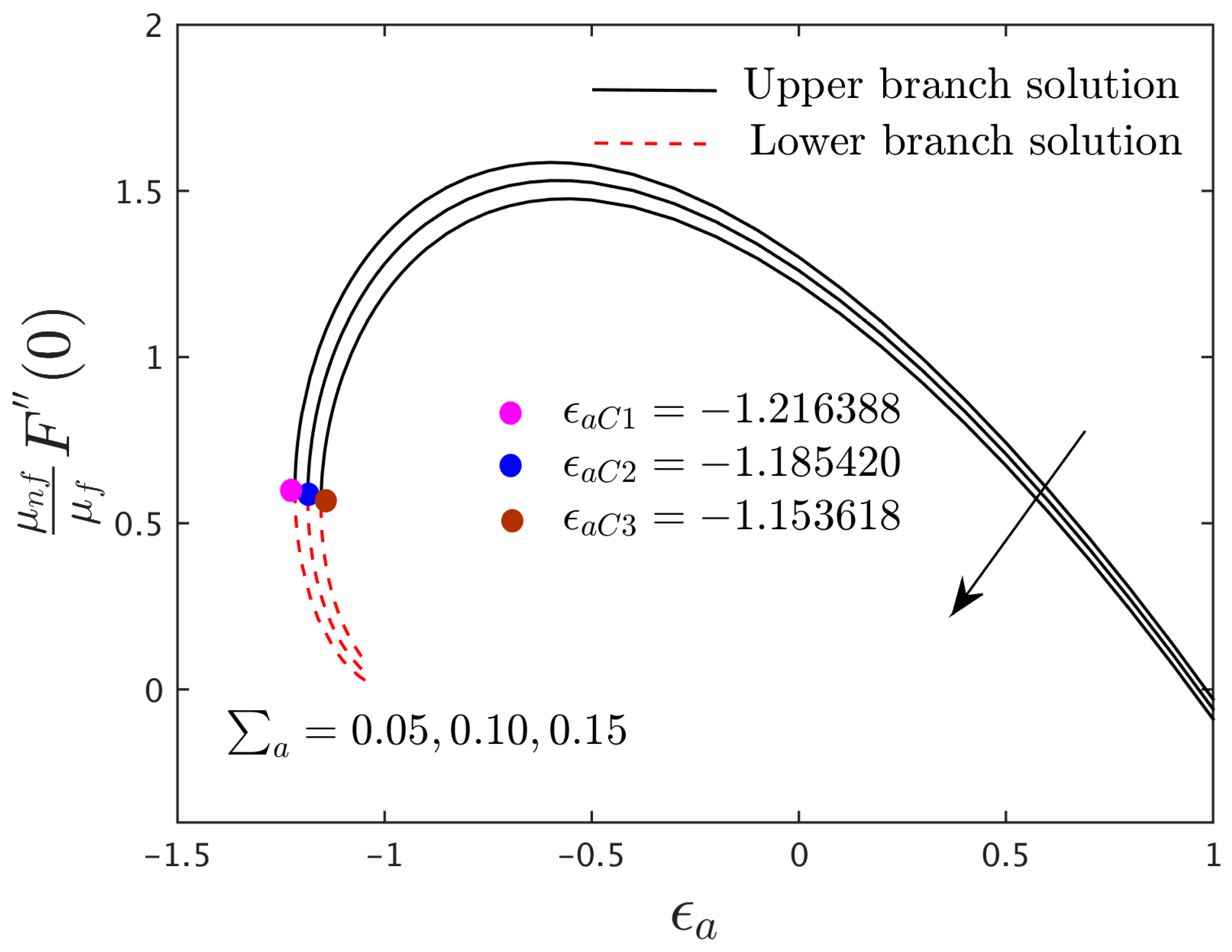
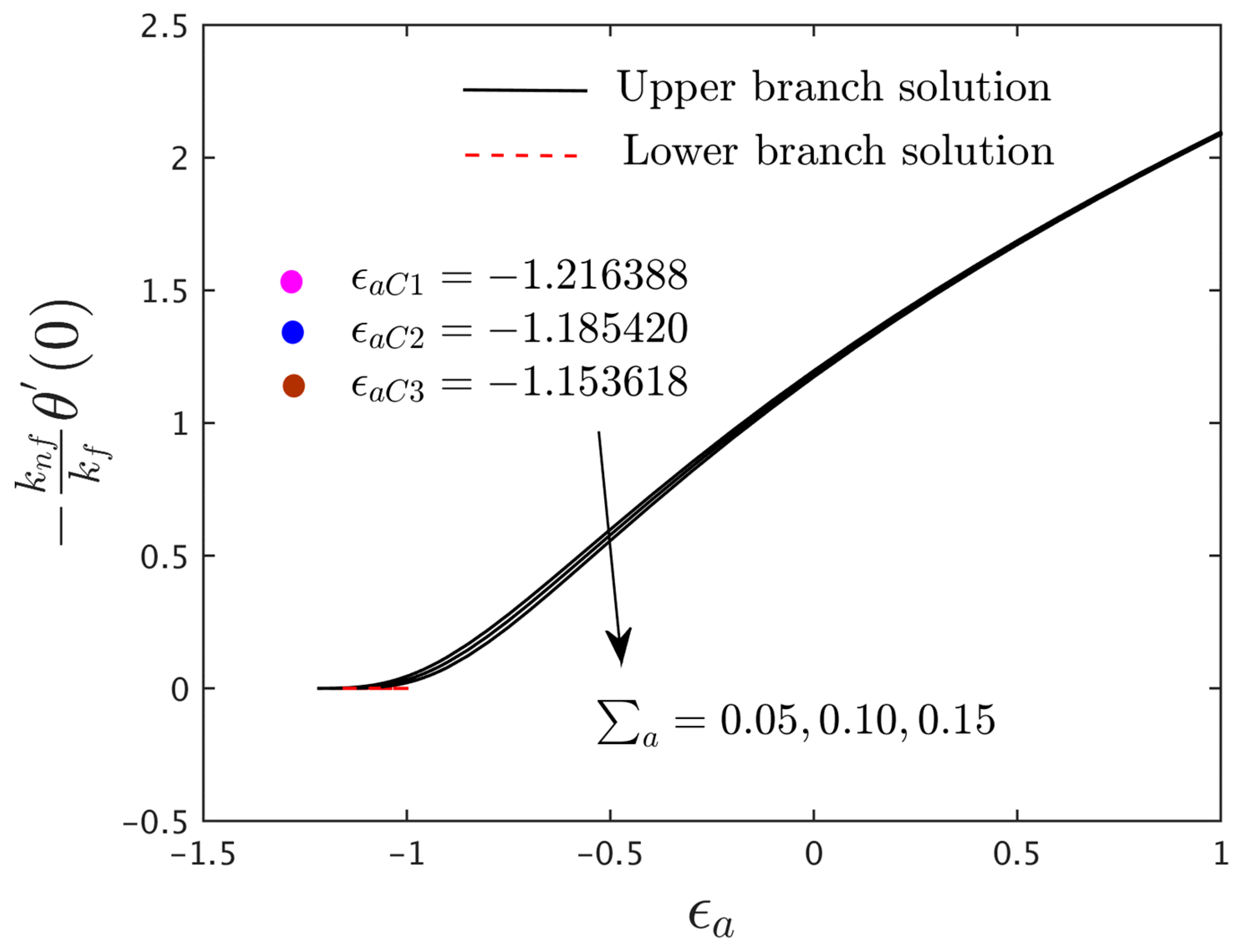
4.2. Research Physical Explanation of the Gradients

The variations of the friction factor and heat transfer versus the stretching/shrinking parameter ${\epsilon }_a$ are shown in Figure 2, Figure 3, Figure 4 and Figure 5 for different values of the nanoparticle volume fraction $\phi$ and the magnetic factor ${\mathrm{\Sigma }}_a$. These graphs demonstrate that there are regions of no solutions for ${\epsilon }_a<{\epsilon }_{aC}<0$, unique solutions for ${\epsilon }_a>-1$, and dual solutions for ${\epsilon }_{aC}<{\epsilon }_a\le -1$, where ${\epsilon }_{aC}$ is the critical value of ${\epsilon }_a$. It should also be noted that the branch of the first solution to the problems of the friction factor and the heat-transport rate are stable and physically feasible, whereas the second alternatives are not. We will not rehash the processes for demonstrating these due to the fact that they have already been covered by the researchers such as Weidman et al. [43] and Khan et al. [44] quite recently. The outcomes shown in Figure 2, which also shows that the friction factor has a value of zero when ${\epsilon }_a=1$. This is caused by the absence of friction at the fluid–solid interface, which occurs when the fluid and solid boundaries move at the same speed. For ${\epsilon }_a>1$ and ${\epsilon }_a<1$, the values of the friction factor are positive and negative, respectively. Generally, a positive value of the friction factor designates that the liquid pulls on the solid barrier, whereas a negative value indicates the reverse phenomenon. In addition, Figure 2 and Figure 3 reveal that the developing effect of the nanoparticle volume fraction causes the shear stress and heat transfer for the UB and LB solutions to increase. Physically, the thermal conductivity of the fluid is very high due to the existence of the nanoparticle’s volume fraction, and as a result the heat transfer escalates. Based on the computations, the following critical values, such as ${\epsilon }_{aC1}=-1.216388$, ${\epsilon }_{aC2}=-1.217519$, and ${\epsilon }_{aC3}=-1.218586$, are obtained for the three distinct values of $\phi$. As is noted in the graphs, the larger values of $\phi$ develop the domain of the output existence versus the movable parameter, which causes the enrichment the magnitude of the critical values. This pattern enables us to identify that the boundary layer separation is slower due to higher values of $\phi$. The impacts of the magnetic factor on the friction factor and heat transfer on the existence of graphene oxide nanoparticles for the UB and LB solutions are illustrated in the respective Figure 4 and Figure 5. The outcomes reveal that the friction factor and heat transfer decay for the UB solutions due to the sophisticated impact of the magnetic factor. Meanwhile, the heat transfer behaves progressively for the LB solutions due to the superior impressions of the magnetic factor, but the friction factor performs similarly to in the upper-branch solutions. Additionally, the magnetic parameter is carefully chosen to produce the bifurcation value, which is expressed in the form of numbers such as ${\epsilon }_{aC1}=-1.216388$, ${\epsilon }_{aC2}=-1.185420$, and ${\epsilon }_{aC3}=-1.153618$, respectively. From these critical values, it is noticed that the pattern of the bifurcation reduces in relationships of magnitude. This tendency further specifies that the breakdown of the lower branch enriches with higher impressions of magnetic factor.

Figure 2. The friction factor versus ${\epsilon }_a$ for the numerous values of $\phi$ when ${\mathrm{Pr}}_a=1.0$, $S{c}_a=10.0$, $\mathrm{Pr}=6.2$, ${\mathrm{\Sigma }}_a=0.05$, and ${\gamma }_s=0.5$.

Figure 2. The friction factor versus ${\epsilon }_a$ for the numerous values of $\phi$ when ${\mathrm{Pr}}_a=1.0$, $S{c}_a=10.0$, $\mathrm{Pr}=6.2$, ${\mathrm{\Sigma }}_a=0.05$, and ${\gamma }_s=0.5$.

Figure 3. The rate of heat transfer versus ${\epsilon }_a$ for the numerous values of $\phi$ when ${\mathrm{Pr}}_a=1.0$, $S{c}_a=10.0$, $\mathrm{Pr}=6.2$, ${\mathrm{\Sigma }}_a=0.05$, and ${\gamma }_s=0.5$.

Figure 3. The rate of heat transfer versus ${\epsilon }_a$ for the numerous values of $\phi$ when ${\mathrm{Pr}}_a=1.0$, $S{c}_a=10.0$, $\mathrm{Pr}=6.2$, ${\mathrm{\Sigma }}_a=0.05$, and ${\gamma }_s=0.5$.

Figure 4. The friction factor versus ${\epsilon }_a$ for the numerous values of ${\mathrm{\Sigma }}_a$ when ${\mathrm{Pr}}_a=1.0$, $S{c}_a=10.0$, $\mathrm{Pr}=6.2$, $\phi =0.025$, and ${\gamma }_s=0.5$.

Figure 4. The friction factor versus ${\epsilon }_a$ for the numerous values of ${\mathrm{\Sigma }}_a$ when ${\mathrm{Pr}}_a=1.0$, $S{c}_a=10.0$, $\mathrm{Pr}=6.2$, $\phi =0.025$, and ${\gamma }_s=0.5$.

Figure 5. The rate of heat transfer versus ${\epsilon }_a$ for the numerous values of ${\mathrm{\Sigma }}_a$ when ${\mathrm{Pr}}_a=1.0$, $S{c}_a=10.0$, $\mathrm{Pr}=6.2$, $\phi =0.025$, and ${\gamma }_s=0.5$.

Figure 5. The rate of heat transfer versus ${\epsilon }_a$ for the numerous values of ${\mathrm{\Sigma }}_a$ when ${\mathrm{Pr}}_a=1.0$, $S{c}_a=10.0$, $\mathrm{Pr}=6.2$, $\phi =0.025$, and ${\gamma }_s=0.5$.

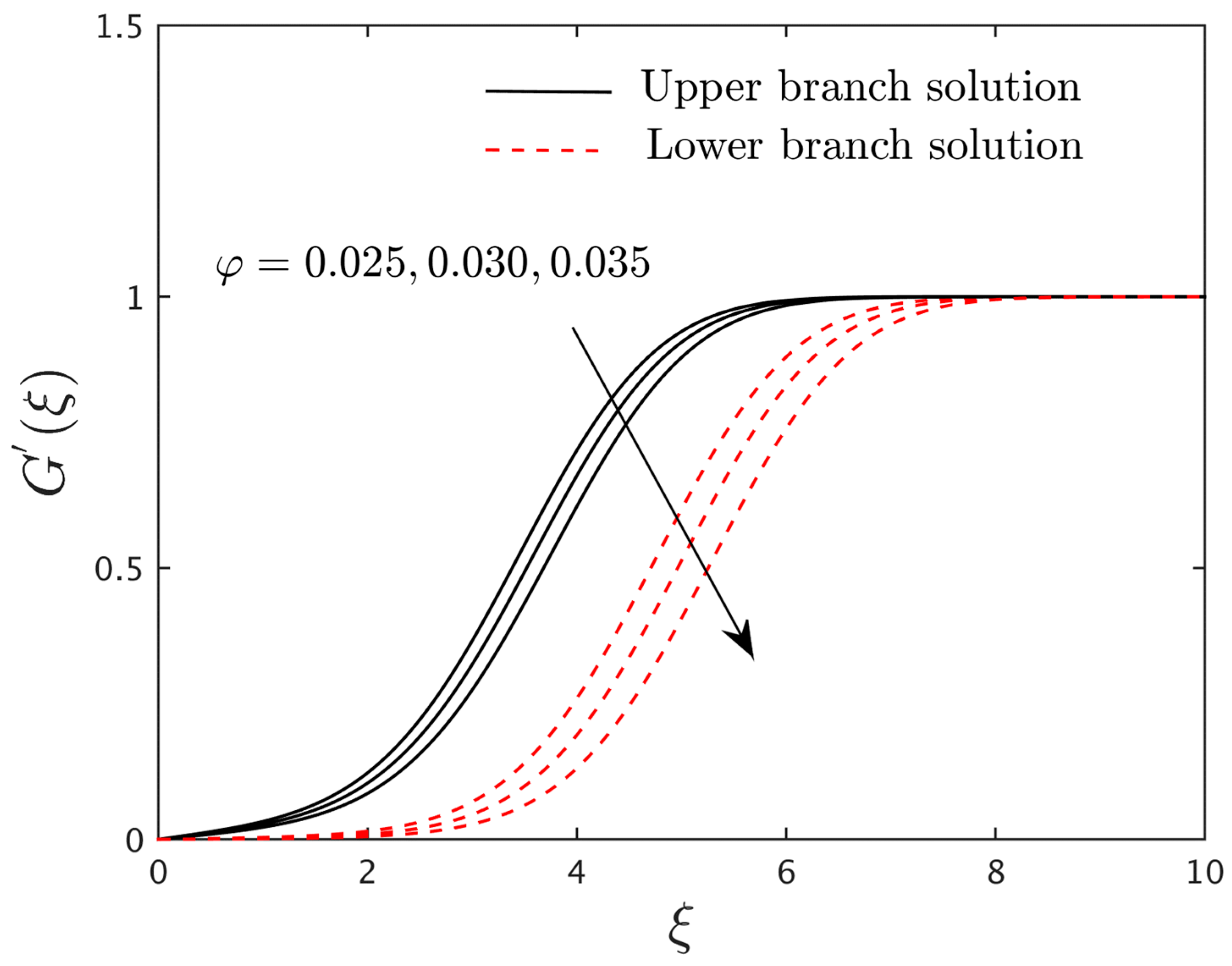
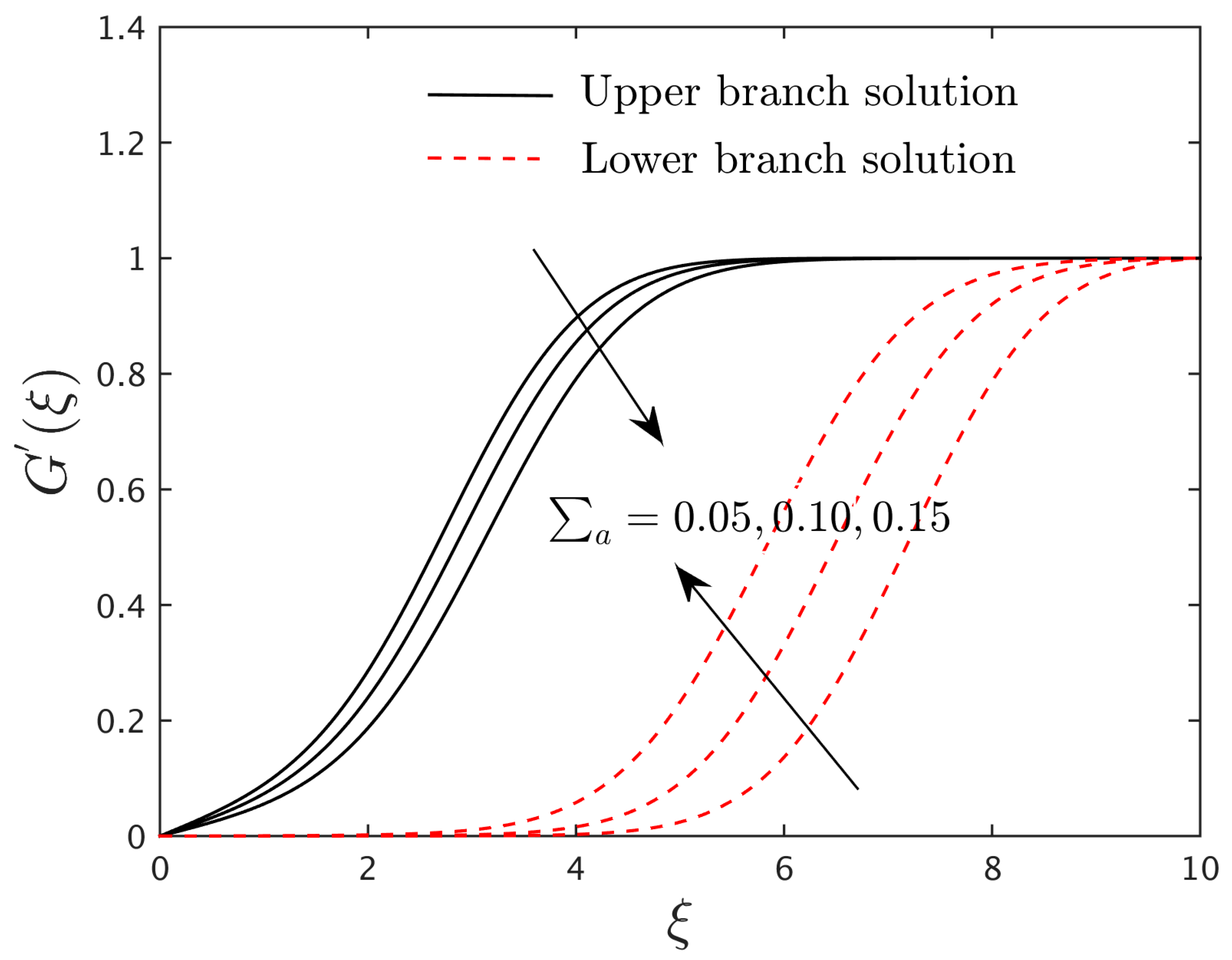
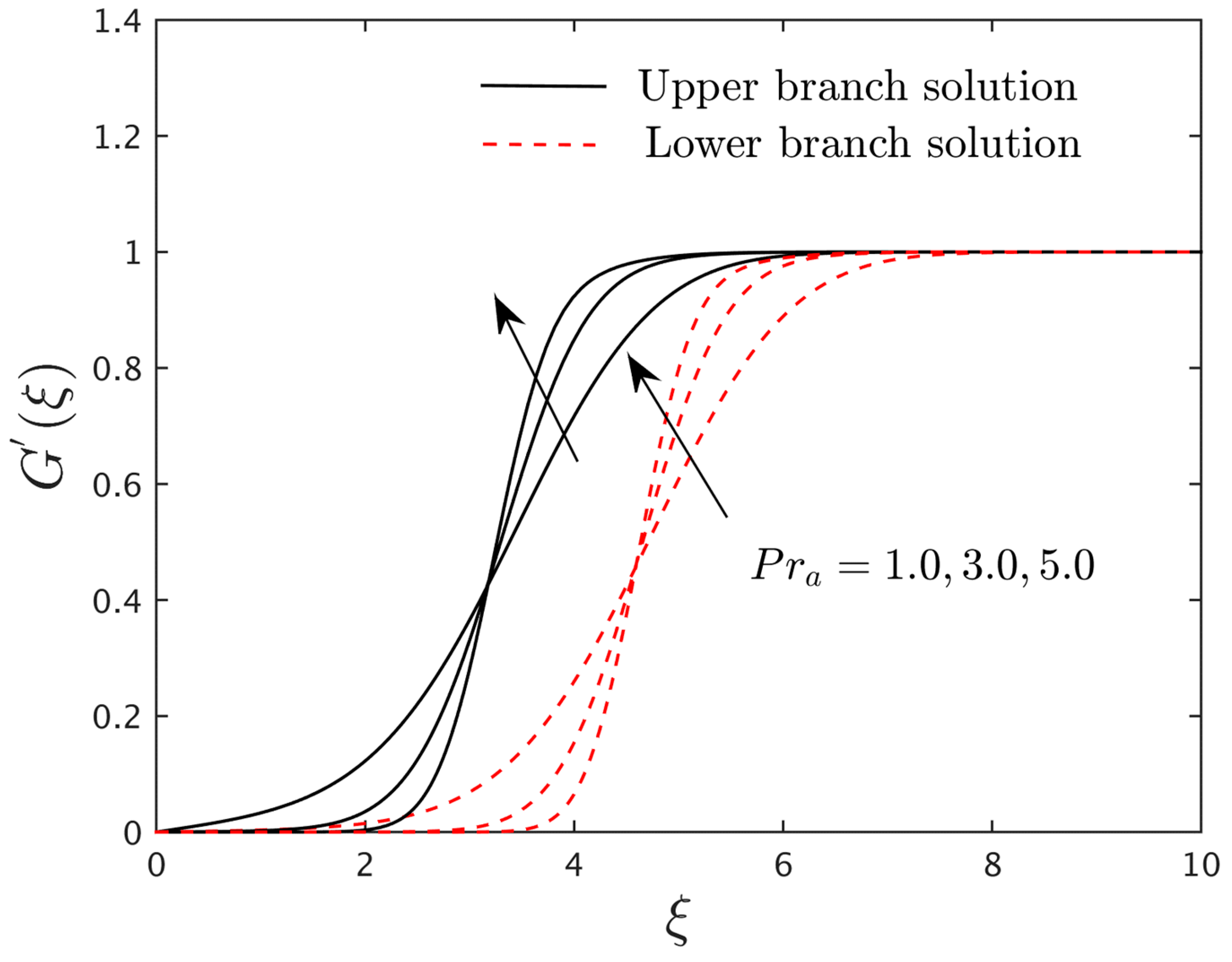
4.3. Research Physical Explanation of the Velocity and Induced Magnetic Profiles

Figure 6, Figure 7, Figure 8, Figure 9 and Figure 10 display the velocity profiles and the induced magnetic profiles in the existence of the graphene oxide nanoparticles for the UB and LB outputs with the change value of the solid volume fraction of the nanoparticle $\phi$, the magnetic parameter ${\mathrm{\Sigma }}_a$, and ${\mathrm{Pr}}_a$. The fact that all of the sample profiles asymptotically satisfy the far-field boundary conditions (28) provides evidence for the obtained numerical outcomes. From Figure 6 and Figure 7, it is realized that as the values of $\phi$ upsurge, both the fluid velocities and the induced magnetic profiles reduce for both the UB and LB outputs. Furthermore, the momentum and induced magnetic BLT shrink with the higher influences of $\phi$. Physically, the higher impacts of the nanoparticles create a strong viscous influence due to which the motion of the fluid and the induced magnetic velocity decline. In contrast, as the values of the magnetic factor ${\mathrm{\Sigma }}_a$ intensify, the motion of the fluid velocity and the induced magnetic profile decrease for the upper-branch solutions, while for the branch of lower solutions these findings are vice versa (see Figure 8 and Figure 9). However, the space between the curves of the lower branch is better than the curves of the upper-branch solutions. Usually, this tendency is seen as being owed to the well-known fact that a larger magnetic influence generates strong Lorentz forces, and as a result the induced magnetic profiles slow down or shrink. On the other hand, the impact of ${\mathrm{Pr}}_a$ on the induced magnetic profiles for the UB and LB outputs is depicted in Figure 10. Here, we can notice that the induced magnetic profiles initially decline and then uplift for both UB and LB outcomes, with higher impacts of ${\mathrm{Pr}}_a$. The outcomes of the given profile with varying ${\mathrm{Pr}}_a$ demonstrate more fascinating behavior as compared with the aforementioned figures.

Figure 6. The velocity profiles $F\prime \left(\xi \right)$ for the several values of $\phi$ when ${\mathrm{Pr}}_a=1.0$, $S{c}_a=10.0$, $\mathrm{Pr}=6.2$, ${\mathrm{\Sigma }}_a=0.05$, and ${\gamma }_s=0.5$.

Figure 6. The velocity profiles $F\prime \left(\xi \right)$ for the several values of $\phi$ when ${\mathrm{Pr}}_a=1.0$, $S{c}_a=10.0$, $\mathrm{Pr}=6.2$, ${\mathrm{\Sigma }}_a=0.05$, and ${\gamma }_s=0.5$.

Figure 7. The induced magnetic profiles $G\prime \left(\xi \right)$ for the numerous values of $\phi$ when ${\mathrm{Pr}}_a=1.0$, $S{c}_a=10.0$, $\mathrm{Pr}=6.2$, ${\mathrm{\Sigma }}_a=0.05$, and ${\gamma }_s=0.5$.

Figure 7. The induced magnetic profiles $G\prime \left(\xi \right)$ for the numerous values of $\phi$ when ${\mathrm{Pr}}_a=1.0$, $S{c}_a=10.0$, $\mathrm{Pr}=6.2$, ${\mathrm{\Sigma }}_a=0.05$, and ${\gamma }_s=0.5$.

Figure 8. The velocity profiles $F\prime \left(\xi \right)$ for the numerous values of ${\mathrm{\Sigma }}_a$ when ${\mathrm{Pr}}_a=1.0$, $S{c}_a=10.0$, $\mathrm{Pr}=6.2$, $\phi =0.025$, and ${\gamma }_s=0.5$.

Figure 8. The velocity profiles $F\prime \left(\xi \right)$ for the numerous values of ${\mathrm{\Sigma }}_a$ when ${\mathrm{Pr}}_a=1.0$, $S{c}_a=10.0$, $\mathrm{Pr}=6.2$, $\phi =0.025$, and ${\gamma }_s=0.5$.

Figure 9. The induced magnetic profiles $G\prime \left(\xi \right)$ for the numerous values of ${\mathrm{\Sigma }}_a$ when ${\mathrm{Pr}}_a=1.0$, $S{c}_a=10.0$, $\mathrm{Pr}=6.2$, $\phi =0.025$, and ${\gamma }_s=0.5$.

Figure 9. The induced magnetic profiles $G\prime \left(\xi \right)$ for the numerous values of ${\mathrm{\Sigma }}_a$ when ${\mathrm{Pr}}_a=1.0$, $S{c}_a=10.0$, $\mathrm{Pr}=6.2$, $\phi =0.025$, and ${\gamma }_s=0.5$.

Figure 10. The induced magnetic profiles $G\prime \left(\xi \right)$ for the numerous values of ${\mathrm{Pr}}_a$ when ${\mathrm{\Sigma }}_a=0.05$, $S{c}_a=10.0$, $\mathrm{Pr}=6.2$, $\phi =0.025$, and ${\gamma }_s=0.5$.

Figure 10. The induced magnetic profiles $G\prime \left(\xi \right)$ for the numerous values of ${\mathrm{Pr}}_a$ when ${\mathrm{\Sigma }}_a=0.05$, $S{c}_a=10.0$, $\mathrm{Pr}=6.2$, $\phi =0.025$, and ${\gamma }_s=0.5$.

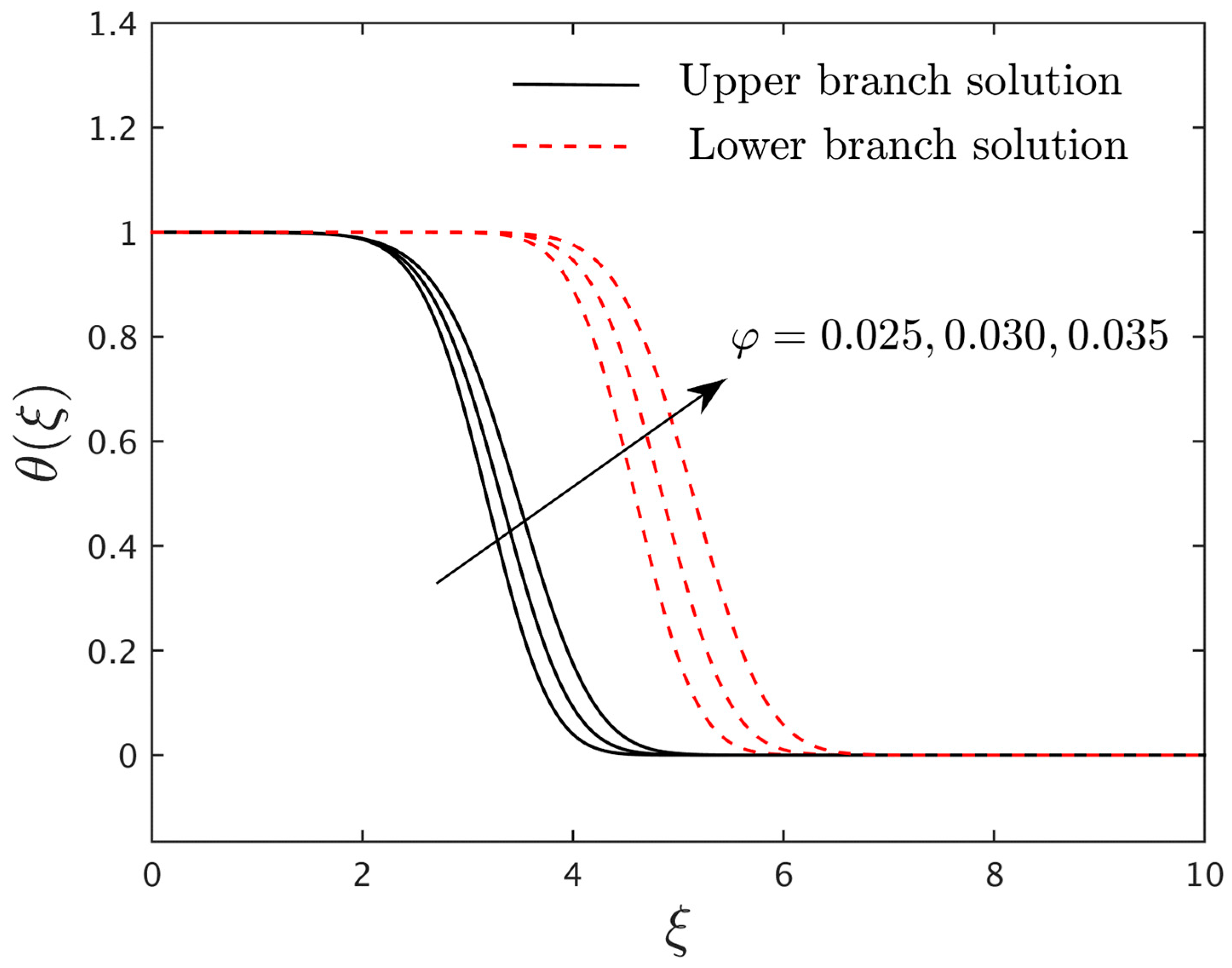
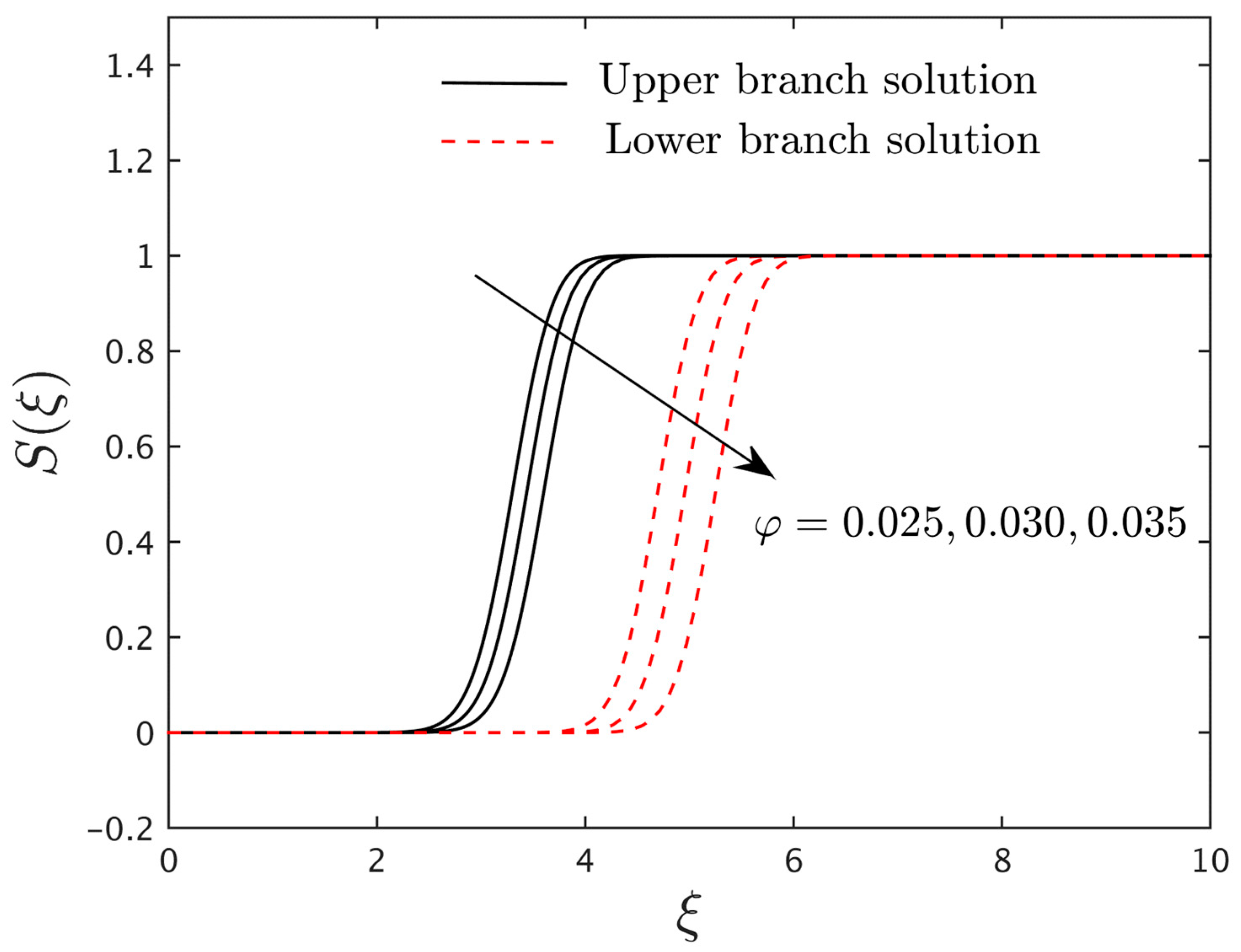
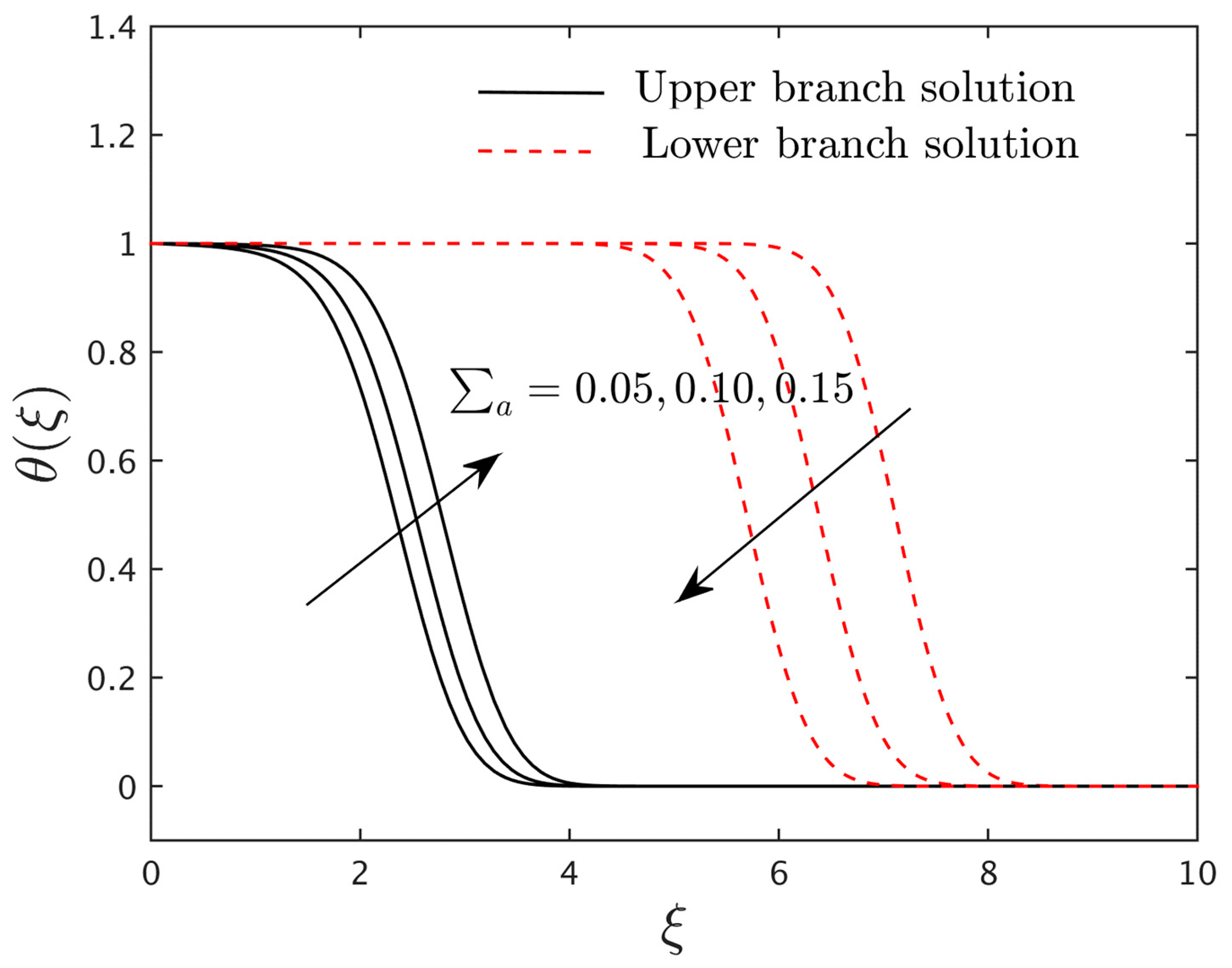
4.4. Research Physical Explanation of the Temperature and Concentration Profiles

The impacts of the nanoparticle volume fraction $\phi$ on the temperatures and concentration profiles for the UB and LB outputs against $\xi$ are presented in Figure 11 and Figure 12, respectively. From both plots, it is noticed that as the values of $\phi$ escalates, the temperature curves enhance for both branches, while the concentration profiles diminish. This physical behavior is due to the fact that as the nanoparticle volume fraction augments, the thermal conductivity rises, and as a result the temperature and the thickness of the thermal boundary layer develop. The effects of magnetic factor ${\mathrm{\Sigma }}_a$ and the Schmidt number $S{c}_a$ on the temperatures and concentration profiles in the presence of graphene oxide nanoparticles are described in Figure 13, Figure 14 and Figure 15, respectively. From Figure 13 and Figure 14, we see that as the value of ${\mathrm{\Sigma }}_a$ upsurges, the temperature and concentration profile improve and reduce for the upper-branch solutions, respectively, while for the branch of lower solution both profiles behave oppositely. On the other hand, the concentration profiles enlarge for two altered branches of output with the superior impacts of Schmidt number (see Figure 15). In other words, it is the ratio-to-mass-momentum transfer rate. From a physical point of view, it is found that increasing the heat-to-mass diffusion ratio causes the former diffusion (mass diffusivity) to replace the latter (momentum diffusivity), which results in a reduction in the mass distribution. Thus, the concentration profiles and the concentration boundary layer thicknesses decline.

Figure 11. The temperature profiles $\theta \left(\xi \right)$ for the numerous values of $\phi$ when ${\mathrm{Pr}}_a=1.0$, $S{c}_a=10.0$, $\mathrm{Pr}=6.2$, ${\mathrm{\Sigma }}_a=0.05$, and ${\gamma }_s=0.5$.

Figure 11. The temperature profiles $\theta \left(\xi \right)$ for the numerous values of $\phi$ when ${\mathrm{Pr}}_a=1.0$, $S{c}_a=10.0$, $\mathrm{Pr}=6.2$, ${\mathrm{\Sigma }}_a=0.05$, and ${\gamma }_s=0.5$.

Figure 12. The concentration profiles $S\left(\xi \right)$ for the numerous values of $\phi$ when ${\mathrm{Pr}}_a=1.0$, $S{c}_a=10.0$, $\mathrm{Pr}=6.2$, ${\mathrm{\Sigma }}_a=0.05$, and ${\gamma }_s=0.5$.

Figure 12. The concentration profiles $S\left(\xi \right)$ for the numerous values of $\phi$ when ${\mathrm{Pr}}_a=1.0$, $S{c}_a=10.0$, $\mathrm{Pr}=6.2$, ${\mathrm{\Sigma }}_a=0.05$, and ${\gamma }_s=0.5$.

Figure 13. The temperature profiles $\theta \left(\xi \right)$ for the numerous values of ${\mathrm{\Sigma }}_a$ when ${\mathrm{Pr}}_a=1.0$, $S{c}_a=10.0$, $\mathrm{Pr}=6.2$, $\phi =0.025$, and ${\gamma }_s=0.5$.

Figure 13. The temperature profiles $\theta \left(\xi \right)$ for the numerous values of ${\mathrm{\Sigma }}_a$ when ${\mathrm{Pr}}_a=1.0$, $S{c}_a=10.0$, $\mathrm{Pr}=6.2$, $\phi =0.025$, and ${\gamma }_s=0.5$.

Figure 14. The concentration profiles $S\left(\xi \right)$ for the numerous values of ${\mathrm{\Sigma }}_a$ when ${\mathrm{Pr}}_a=1.0$, $S{c}_a=10.0$, $\mathrm{Pr}=6.2$, $\phi =0.025$, and ${\gamma }_s=0.5$.

Figure 14. The concentration profiles $S\left(\xi \right)$ for the numerous values of ${\mathrm{\Sigma }}_a$ when ${\mathrm{Pr}}_a=1.0$, $S{c}_a=10.0$, $\mathrm{Pr}=6.2$, $\phi =0.025$, and ${\gamma }_s=0.5$.

Figure 15. The concentration profiles $S\left(\xi \right)$ for the numerous values of $S{c}_a$ when ${\mathrm{Pr}}_a=1.0$, ${\mathrm{\Sigma }}_a=0.05$, $\mathrm{Pr}=6.2$, $\phi =0.025$, and ${\gamma }_s=0.5$.

Figure 15. The concentration profiles $S\left(\xi \right)$ for the numerous values of $S{c}_a$ when ${\mathrm{Pr}}_a=1.0$, ${\mathrm{\Sigma }}_a=0.05$, $\mathrm{Pr}=6.2$, $\phi =0.025$, and ${\gamma }_s=0.5$.

5. Conclusions

The present study was carried out to investigate the stagnation-point flow of a water-based graphene oxide nanoparticles flow over a movable surface while experiencing the significant impact of an induced magnetic field and a homogeneous–heterogeneous chemical reaction. By exercising the similarity technique, the leading equations and the additional boundary constraints were first translated into dimensionless form. The bvp4c method was then used to numerically solve the resulting equations. The impacts of the pertinent factors on the fluid flow, induced magnetic profiles, temperature profiles, concentration profiles, heat transfer, and friction factors are depicted in various distinct graphs. The notable outcomes of the present study are as follows:

• The results for the shrinking sheet are found to be non-unique in contrast to their stretching sheet counterpart.
• The friction factor and heat transfer have boosted up for both solution branches as a result of the addition of graphene oxide nanoparticles to the base water fluid, and this impression is meaningfully accentuated as the nanoparticle volume fraction rises.
• For growing values of the nanoparticle volume fraction, the friction factors upsurge by almost 0.96% and 0.66% for the upper- and lower-branch solutions, respectively.
• The higher impact of the magnetic factor reduces the friction factor and the heat transfer for the branch of the upper solutions, while the patterns are altered for the second-branch solutions.
• The friction factor and heat transfer decline about to 9.58% and 69.4% for the respective branch of upper solutions due to higher impacts of magnetic parameter, while they escalate by almost 19.32% and 31.5% for the branch of lower solutions, respectively.
• The magnitude of the critical values upsurges as the values of $\phi$ escalates, while it shrinks with higher impacts of the magnetic factor.
• The heat-transport phenomenon uplifts up to 11.71% for the upper-branch solutions and 21.8% for the branch of lower-branch solutions owing to larger values of $\phi$.
• For the growing values of the nanoparticle volume fraction, the fluid velocity, induced magnetic field, and concentration profiles decline for the two distinct branch solutions, but the temperature profiles abruptly develop.
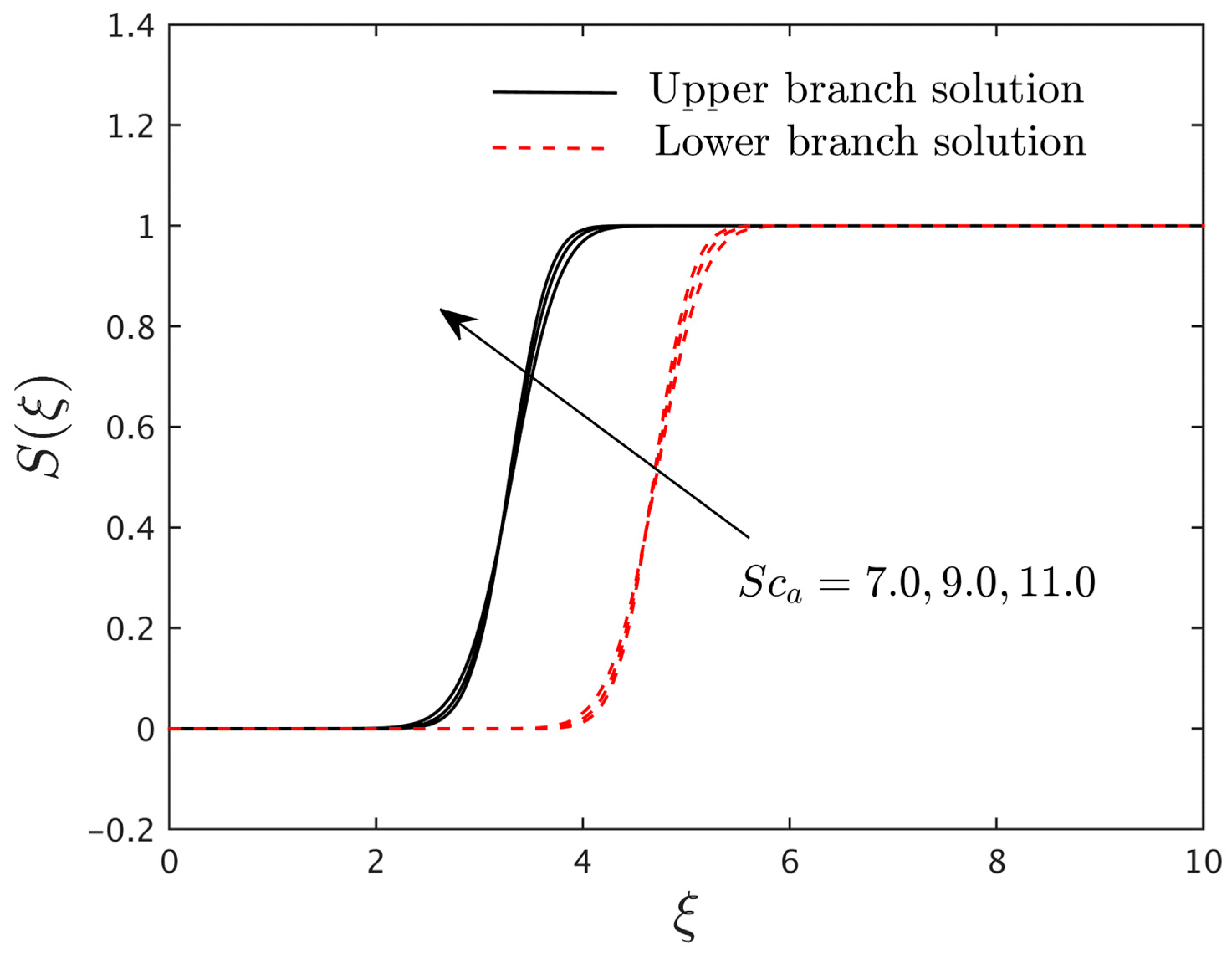
• The concentration profiles are augmented for the two altered outcome branches due to some change values of the Schmidt number.

References

1. Choi, S.U.; Eastman, J.A. Enhancing thermal conductivity of fluids with nanoparticles. In Proceedings of the 1995 International Mechanical Engineering Congress and Exhibition, San Francisco, CA, USA, 12–17 November 1995. [Google Scholar]
2. Khan, W.A.; Pop, I. Boundary-layer flow of a nanofluid past a stretching sheet. Int. J. Heat Mass Transf. 2010, 53, 2477–2483. [Google Scholar] [CrossRef]
3. Bachok, N.; Ishak, A.; Pop, I. Unsteady boundary-layer flow and heat transfer of a nanofluid over a permeable stretching/shrinking sheet. Int. J. Heat Mass Transf. 2012, 55, 2102–2109. [Google Scholar] [CrossRef]
4. Gireesha, B.J.; Mahanthesh, B.; Gorla, R.S.R. Suspended Particle Effect on Nanofluid Boundary Layer Flow Past a Stretching Surface. J. Nanofluids 2014, 3, 267–277. [Google Scholar]
5. Jain, D.S.; Rao, S.S.; Srivastava, A. Rainbow schlieren deflectometry technique for nanofluid-based heat transfer measurements under natural convection regime. Int. J. Heat Mass Transf. 2016, 98, 697–711. [Google Scholar]
6. Rao, S.S.; Srivastava, A. Interferometric study of natural convection in a differentially-heated cavity with Al 2 O 3 –water based dilute nanofluids. Int. J. Heat Mass Transf. 2016, 92, 1128–1142. [Google Scholar]
7. Makinde, O.D.; Mishra, S.R. On Stagnation Point Flow of Variable Viscosity Nanofluids Past a Stretching Surface with Radiative Heat. Int. J. Appl. Comput. Math. 2015, 3, 561–578. [Google Scholar] [CrossRef]
8. Bhatti, M.M.; Mishra, S.R.; Abbas, T.; Rashidi, M.M. A mathematical model of MHD nanofluid flow having gyrotactic microorganisms with thermal radiation and chemical reaction effects. Neural Comput. Appl. 2018, 30, 1237–1249. [Google Scholar]
9. Zuhra, S.; Khan, N.S.; Khan, M.A.; Islam, S.; Khan, W.; Bonyah, E. Flow and heat transfer in water based liquid film fluids dispensed with graphene nanoparticles. Results Phys. 2018, 8, 1143–1157. [Google Scholar] [CrossRef]
10. Khan, U.; Zaib, A.; Shah, Z.; Baleanu, D.; Sherif, E.-S.M. Impact of magnetic field on boundary-layer flow of Sisko liquid comprising nanomaterials migration through radially shrinking/stretching surface with zero mass flux. J. Mater. Res. Technol. 2020, 9, 3699–3709. [Google Scholar] [CrossRef]
11. Zaib, A.; Khan, U.; Khan, I.; Sherif, E.-S.M.; Nisar, K.S.; Seikh, A.H. Impact of Nonlinear Thermal Radiation on the Time-Dependent Flow of Non-Newtonian Nanoliquid over a Permeable Shrinking Surface. Symmetry 2020, 12, 195. [Google Scholar] [CrossRef] [Green Version]
12. Nayak, B.; Mishra, S.R. Squeezing flow analysis of CuO–water and CuO–kerosene-based nanofluids: A comparative study. Pramana J. Phys. 2021, 95, 29. [Google Scholar]
13. Waini, I.; Khan, U.; Zaib, A.; Ishak, A.; Pop, I. Inspection of TiO2-CoFe2O4 nanoparticles on MHD flow toward a shrinking cylinder with radiative heat transfer. J. Mol. Liq. 2022, 361, 119615. [Google Scholar] [CrossRef]
14. Glauert, M.B. The boundary layer on a magnetized plate. J. Fluid Mech. 1962, 12, 625–638. [Google Scholar] [CrossRef]
15. Takhar, H.; Chamkha, A.; Nath, G. Unsteady flow and heat transfer on a semi-infinite flat plate with an aligned magnetic field. Int. J. Eng. Sci. 1999, 37, 1723–1736. [Google Scholar]
16. Alom, M.M.; Rafiqul, I.M.; Rahman, F. Steady heat and mass transfer by mixed convection flow from a vertical porous plate with induced magnetic field, constant heat and mass fluxes. Thammasat. Int. J. Sci. Technol. 2008, 13, 1–13. [Google Scholar]
17. Ahmed, S.; Chamkha, A.J. Effects of chemical reaction, heat and mass transfer and radiation on MHD flow along a vertical porous wall in the present of induced magnetic field. Int. J. Ind. Math. 2009, 2, 245–261. [Google Scholar]
18. Bég, O.A.; Bakier, A.; Prasad, V.; Zueco, J.; Ghosh, S. Nonsimilar, laminar, steady, electrically-conducting forced convection liquid metal boundary layer flow with induced magnetic field effects. Int. J. Therm. Sci. 2009, 48, 1596–1606. [Google Scholar]
19. Ghosh, S.K.; Bég, O.A.; Zueco, J. Hydromagnetic free convection flow with induced magnetic field effects. Meccanica 2009, 45, 175–185. [Google Scholar]
20. Ali, F.M.; Nazar, R.; Arifin, N.; Pop, I. MHD stagnation-point flow and heat transfer towards stretching sheet with induced magnetic field. Appl. Math. Mech. 2011, 32, 409–418. [Google Scholar]
21. Gireesha, B.; Mahanthesh, B.; Shivakumara, I.; Eshwarappa, K. Melting heat transfer in boundary layer stagnation-point flow of nanofluid toward a stretching sheet with induced magnetic field. Eng. Sci. Technol. Int. J. 2016, 19, 313–321. [Google Scholar] [CrossRef] [Green Version]
22. Sheikholeslami, M.; Rokni, H.B. Nanofluid two phase model analysis in existence of induced magnetic field. Int. J. Heat Mass Transf. 2017, 107, 288–299. [Google Scholar] [CrossRef]
23. Hou, E.; Hussain, A.; Rehman, A.; Baleanu, D.; Nadeem, S.; Matoog, R.T.; Khan, I.; Sherif, E.-S.M. Entropy generation and induced magnetic field in pseudoplastic nanofluid flow near a stagnant point. Sci. Rep. 2021, 11, 23736. [Google Scholar] [CrossRef] [PubMed]
24. Williams, W.R.; Stenzel, M.T.; Song, X.; Schmidt, L.D. Bifurcation behaviour in homogeneous-heterogeneous combustion. I. Experimental results over platinum. Combust. Flame 1991, 84, 277–291. [Google Scholar] [CrossRef]
25. Williams, W.R.; Zhao, J.; Schmidt, L.D. Ignition and extinction of surface and homogeneous oxidation of NH3 and CH4. AIChE J. 1991, 37, 641–649. [Google Scholar] [CrossRef]
26. Song, X.; Williams, W.R.; Schmidt, L.D.; Aris, R. Bifurcation behaviour in homogeneous-heterogeneous combustion. II. Computations for stagnation-point flow. Combust. Flame 1991, 84, 292–311. [Google Scholar] [CrossRef]
27. Song, X.; Schmidt, L.; Aris, R. Steady states and oscillations in homogeneous—Heterogeneous reaction systems. Chem. Eng. Sci. 1991, 46, 1203–1215. [Google Scholar] [CrossRef]
28. Song, X.; Schmidt, L.D.; Aris, R. The ignition criteria for stagnation-point flow: Semenov–Frank–Kamenetskii or van’t Hoff. Combust. Sci. Technol. 1991, 75, 311–331. [Google Scholar] [CrossRef]
29. Ikeda, H.; Libby, P.A.; Williams, F.A.; Sato, J. Catalytic combustion of hydrogen-air mixtures in stagnation flows. Combust. Flame 1993, 93, 138–148. [Google Scholar] [CrossRef]
30. Chaudhary, M.A.; Merkin, J.H. A simple isothermal model for homogeneous-heterogeneous reactions in boundary-layer flow. I Equal diffusivities. Fluid Dyn. Res. 1995, 16, 311–333. [Google Scholar] [CrossRef]
31. Chaudhary, M.A.; Merkin, J.H. A simple isothermal model for homogeneous-heterogeneous reactions in boundary-layer flow. II Different diffusivities for reactant and autocatalyst. Fluid Dyn. Res. 1995, 16, 335–359. [Google Scholar] [CrossRef]
32. Bachok, N.; Ishak, A.; Pop, I. On the stagnation-point flow towards a stretching sheet with homogeneous–heterogeneous reactions effects, Commun. Nonlinear Sci. Numer. Simulat. 2011, 16, 4296–4302. [Google Scholar] [CrossRef]
33. Ibrahim, W. The effect of induced magnetic field and convective boundary condition on MHD stagnation point flow and heat transfer of upper-convected Maxwell fluid in the presence of nanoparticle past a stretching sheet. Propuls. Power Res. 2016, 5, 164–175. [Google Scholar] [CrossRef] [Green Version]
34. Mahanthesh, B.; Gireesha, B.; Athira, P. Radiated flow of chemically reacting nanoliquid with an induced magnetic field across a permeable vertical plate. Results Phys. 2017, 7, 2375–2383. [Google Scholar] [CrossRef]
35. Jha, B.K.; Aina, B. Impact of induced magnetic field onmagnetohydrodynamic (MHD) natural convection flow in a vertical annular micro-channel in the presence of radial magnetic field. Propuls. Power Res. 2018, 7, 171–181. [Google Scholar] [CrossRef]
36. Goud, B.S.; Kumar, P.P.; Malga, B.S. Induced magnetic field effect on MHD free convection flow in nonconducting and conducting vertical microchannel walls. Heat Transf. 2021, 51, 2201–2218. [Google Scholar] [CrossRef]
37. Kumar, D. Radiation effect on magnetohydrodynamic flow with induced magnetic field and Newtonian heating/cooling: An analytic approach. Propuls. Power Res. 2021, 10, 303–313. [Google Scholar] [CrossRef]
38. Merkin, J. A model for isothermal homogeneous-heterogeneous reactions in boundary-layer flow. Math. Comput. Model. 1996, 24, 125–136. [Google Scholar] [CrossRef]
39. Ho, C.J.; Chen, M.W.; Li, Z.W. Effect of natural convection heat transfer of nanofluid in an enclosure due to uncertainties of viscosity and thermal conductivity. In Proceedings of the ASME-JSME Thermal Engineering Summer Heat Transfer Conference Vancouver, Vancouver, BC, Canada, 8–12 July 2007; pp. 833–841. [Google Scholar]
40. Chu, Y.-M.; Nisar, K.S.; Khan, U.; Kasmaei, H.D.; Malaver, M.; Zaib, A.; Khan, I. Mixed Convection in MHD Water-Based Molybdenum Disulfide-Graphene Oxide Hybrid Nanofluid through an Upright Cylinder with Shape Factor. Water 2020, 12, 1723. [Google Scholar] [CrossRef]
41. Khan, U.; Zaib, A.; Abu Bakar, S.; Ishak, A. Stagnation-point flow of a hybrid nanoliquid over a non-isothermal stretching/shrinking sheet with characteristics of inertial and microstructure. Case Stud. Therm. Eng. 2021, 26, 101150. [Google Scholar] [CrossRef]
42. Khan, U.; Zaib, A.; Ishak, A.; Waini, I.; Raizah, Z.; Prasannakumara, B.C.; Galal, A.M. Dynamics of bio-convection Agrawal axisymmetric flow of water-based Cu-TiO2 hybrid nanoparticles through a porous moving disk with zero mass flux. Chem. Phys. 2022, 561, 111599. [Google Scholar] [CrossRef]
43. Weidman, P.; Kubitschek, D.; Davis, A. The effect of transpiration on self-similar boundary layer flow over moving surfaces. Int. J. Eng. Sci. 2006, 44, 730–737. [Google Scholar] [CrossRef]
44. Khan, U.; Waini, I.; Ishak, A.; Pop, I. Unsteady hybrid nanofluid flow over a radially permeable shrinking/stretching surface. J. Mol. Liq. 2021, 331, 115752. [Google Scholar] [CrossRef]
45. Ridha, A.; Curie, M. Aiding flows non-unique similarity solutions of mixed-convection boundary-layer equations. Z. Angew. Math. Phys. 1996, 47, 341–352. [Google Scholar] [CrossRef]
46. Ishak, A.; Merkin, J.H.; Nazar, R.; Pop, I. Mixed convection boundary layer flow over a permeable vertical surface with prescribed wall heat flux. Z. Angew. Math. Phys. 2008, 59, 100–123. [Google Scholar] [CrossRef]
47. Wang, C. Stagnation flow towards a shrinking sheet. Int. J. Non-linear Mech. 2008, 43, 377–382. [Google Scholar] [CrossRef]
Figure 1. Physical model and coordinate system. (a) Stretching Sheet; (b) Shrinking Sheet.
Magnetochemistry 08 00155 g001