Superparamagnetism of Artificial Glasses Based on Rocks: Experimental Data and Theoretical Modeling

Abstract

Artificial glasses containing nanoscale inclusions of iron oxides, including magnetite and hematite, were obtained via the method of the high-temperature melting of rocks. The main factors influencing the magnetic properties of glasses are the composition of the initial charge and the conditions of cooling of the melt. The data of magnetic granulometry and frequency-field dependencies of magnetic susceptibility showed the presence of a sufficiently large superparamagnetic fraction in the samples. Coordinated theoretical modeling using two independent models that take into consideration possible the chemical inhomogeneity of particles and magnetostatic interaction between them made it possible to calculate hysteresis characteristics corresponding to the experiment and to estimate ferrimagnetic concentrations in the samples, including the superparamagnetic fraction.

1. Introduction

The creation of synthetic analogues of natural objects for a better understanding and use of their properties is one of the most interesting scientific problems. The artificial glasses synthesized from rocks studied in this work are considered analogues of impactites. Coptogenic (impact) rocks are products of transformations of the source rocks (magmatic, metamorphic, and sedimentary), which appeared during a high-speed impact of small cosmic bodies with the Earth resulting in the formation of meteorite craters (astroblemes) [1,2,3]. Some of them are impact glasses, rocks formed through the solidification of homogeneous melts [4,5]. The synthesis of artificial glasses and the study of their petrographic structure, chemical, and phase composition and magnetic properties are actively in demand in the Earth sciences. For example, glassy rock types are widespread among impact rocks. Taking into account the above, natural rocks and their mixtures in various proportions of components, varieties of which are often the material of transformation in the process of impact events, were chosen as the initial charge for melting.

Laboratory reproduction of natural endogenous processes is the main direction of modern experimental and technical petrology [6]. Of course, there is always the problem of unattainability of full analogy between natural processes and their implementation in laboratory conditions, both in terms of time and in terms of the complexity of their route. However, these experiments not only help us understand the phenomena occurring on the Earth; they are also essential for fundamental science and provide an invaluable contribution to solving production problems [7,8,9].

In the field of materials science, the study of glassy substances, which are actively used in the development of various devices and products, plays a major role. For example, the technological areas of melt and glass research include the production of glass fiber, glass ceramics, stone casting, and fused refractories; pyrometallurgy; the growth of some crystals (yttrium–aluminum garnets, etc.); and processes of extraction of ultrapure compounds through zone melting. Materials from gabbro-basalt rocks have high indicators of durability, wear resistance, resistance to shock loads, and chemical stability, while the indicators of properties are preserved both at extremely low and rather high temperatures [10,11]. Due to their unique properties, rock melts can be used to manufacture heat and sound insulators, structural composite and high-temperature materials, shock- and wear-resistant materials, materials for radioactive protection, filters for cleaning waste gases at mining and metallurgical plants, and filters for waste water treatment in various industries [12,13,14,15]. Accordingly, the perspectives for the use of such materials in various industries are extensive; they are used in the aircraft industry, rocket production, the automotive industry, nuclear energy, cryogenics, metallurgy, the chemical industry, and engineering materials production [16,17,18,19].

A special place is occupied by the problem of creating functional nanomaterials, including magnetic ones, which are widely used in information recording and storage systems, magnetic cooling systems, and the creation of permanent magnets and magnetic sensors [20,21,22]. Here, the problem of stabilizing magnetic nanoparticles and, as a consequence, obtaining particles of metals and their oxides embedded in inert, persistent matrices comes to the fore. Two main groups of matrices are used: organic (polymeric) and inorganic [23]. Among the first studies, which systematized the information on nanoscale and cluster metal particles dispersed or chemically bound in polymers, are the monographs [24,25]. Since then, this method of stabilization has been widely developed and new approaches to this problem have appeared: ion-exchange resins, soluble polymers, carbon-chain polymers, polymers containing heteroatoms, polyimines, and block copolymers. Minerals of the zeolite group and other molecular sieves, xerogel and silica gel, highly dispersed SiO₂ and Al₃O₃, nonmagnetic metals, and dispersed carbon are among the varieties of inorganic matrices. Methods for the stabilization of magnetic nanoparticles in glasses continue to be developed [26,27,28,29,30].

Natural and synthetic (artificial) glasses containing atomic clusters or nanoparticles of iron oxides and/or hydroxides are the important object of basic and applied research, including microbiology [31], pearl luster pigment production [32], the simulation of the different atmospheres of the coal gasification process [33], the acidic leaching of metal oxides in nickeliferous ores [34], bioactive glasses for tissue engineering [35,36], iron isotope distribution in terrestrial rocks and meteorites [37], nuclear and toxic waste recycling [38,39], studies on the local coordination environment of cations in silicate glasses and melt [40], the petrology of the surfaces of Venus [41] and Mars [42], the assessment of short- and long-term impacts of ash disposal in different environmental situations [43], etc. The technology of glasses containing iron oxides is similar to industrial production techniques [44].

The aim of this study was to obtain and interpret new data on the physical–chemical and magnetic properties of artificial glasses.

2. Materials and Methods

2.1. Sample Preparation

The samples of artificial glasses were obtained through the high-temperature melting of rocks of different geneses, crystalline shales (s), volcanogenic–sedimentary rocks (a), and psammite–silt–pelitic complexes (c) (sedimentary rocks with significant clay phase content), and their mixtures in different component ratios. The mineral composition of rocks was studied through X-ray powder diffraction (XRD) using a D2 Phaser diffractometer (Bruker, Germany), a software package for the analysis of diffractograms PDXL-2 (Rigaku, Japan), and a database of diffractograms PDF-2 (International Center for Diffraction Data, 2011). Quantitative phase analysis of the source rocks according to the full-profile analysis via the Rietveld method [45] is provided in

Table 1. Quantitative phase analysis of the source rocks used to produce artificial glasses.

Mineral	Content, at. %
	Crystalline Shales	Volcanogenic–Sedimentary Rock	Psammite–Silt–Pelitic Complex
Quartz	5.3	18.0	63.7
Plagioclase	33.2	33.9	8.3
K-feldspar	2.3	1.0	5.4
Pyroxene	-	4.4	1.3
Amphibole	12.8	3.5	-
Mica (muscovite/biotite)	<1	6.0	1.8
Chlorite	8.6	5.1	-
Calcite	17.7	13.2	<1
Dolomite	-	1.3	<1
Epidote	10.7	-	-
Titanite	6.5	-	-
Smectite	1.9	-	-
Heulandite	-	-	2.2
Kaolinite	-	-	15.5
Hematite	-	4.0	1.1
Goethite	-	9.8	-
Rp (%) *	5.4	4.1	2.9

* $R_p=\frac{\sum |y_i^{obs}-y_i^{calc}|}{\sum y_i^{obs}}$ is a convergence factor of calculated and experimental X-ray profiles and $y_i$ is the intensity at each experimental point of the X-ray diffraction pattern.

.

Naturally, the conditions for obtaining artificial glasses available for our experiments do not reproduce the conditions that arise during an impact event. However, they can cover one of the most important temperature ranges in which the main processes of glass transition and crystallization occur. According to the estimates of Masaitis et al. [46], the temperature range for the complete melting of crystalline rocks is 1200–3000 °C, and for partial melting with the formation of many characteristic impact melt rocks, it is 900–1500 °C. However, it is important that the intensity of thermal transformation is directly dependent on the degree of previous shock compression, i.e., degree of fragmentation of rocks. This can reduce the melting point to 950–750 °C. These features of the melting of rocks are reflected in a number of works [47,48,49,50].

The melting of rocks was carried out at the experimental base of the Department of Glass and Ceramics Technology of the Belarusian State Technological University (BSTU). The charge crushed with a BB 50 laboratory jaw crusher (Retsch, Germany) to a fraction < 1.0 mm was melted in corundum crucibles (with a volume of 100 cm³) in a gas flame furnace with turbulent movement of the flame and forced air supply to combustion at a maximum temperature 1515 ± 5 °C. The gas medium was oxidizing, with an excess air ratio of 1.08–1.13. The crucibles were placed in the furnace before heating. Reaching the maximum temperature took about 4 h. Then, part of the crucibles was removed from the furnace and immediately immersed in water. In nature, a wide range of cooling conditions is realized, from fractions of a second to thousands of years; therefore, within the framework of a laboratory experiment, the two most typical cases were selected [51]: sufficiently fast and sufficiently slow. Thus, fast (w) cooling (duration~1 s) of the melt was performed. Slow (f) cooling was ensured through the cooling of crucibles together with the furnace, with a cooling duration~10⁵ s. Further in the paper, we will indicate in the identifiers of artificial glass samples the name of the charge composition and the duration of cooling. In the case of mixtures of rocks, the weight fraction of the corresponding phase is indicated in the upper index in grams. For example, sample a³⁰s¹⁰c⁵f was cooled in a furnace, and the initial charge contained 30 g of volcanogenic–sedimentary rock, 10 g of shales, and 5 g of psammite–silt–pelitic component. In total, 20 samples were synthesized.

2.2. Methods for Physical, Chemical, and Magnetic Characterization

The study of magnetic properties of the samples included measurements of the initial magnetic susceptibility χ at the three frequencies (976, 3904, and 15,616 Hz) at a magnetic field strength amplitude of 200 A/m using a MFK1-FA magnetic susceptibility bridge (AGICO, Brno-Královo Pole, Czech Republic) and plotting hysteresis loops and demagnetization curves of remanence at the maximum field of 1.8 T at room temperature (Lake Shore 7410 vibrating sample magnetometer, Lake Shore Cryotronics Inc., Westerville, OH, USA) while measuring the values of saturation magnetization M_s, saturation remanence M_rs, coercive force H_c, and remanence coercivity H_cr. It should be noted that M_rs is obtained when constructing hysteresis curves by decreasing the external magnetic field from the saturation field to zero. If a field of the opposite direction is applied, then, at the value of the field H_c, M_rs is compensated. However, when the field is switched off in the case of a reversible process, the remanence takes the same value. In order to destroy M_rs, it is possible to increase the field of the opposite direction by ΔH, in a stepwise manner, returning after each step to the remaining fraction of the remanence. Consequently, at some field H_cr, the destruction of M_rs occurs [52]. Thus, H_c is a characteristic of the coercivity of the ensemble of particles as a whole, and H_cr shows the coercivity (remagnetization field) of a single “averaged” particle.

Scanning electron microscopy (SEM) and energy-dispersive X-ray spectroscopy (EDX) were performed to estimate the morphological features and the element composition of the samples. The study was carried out with the use of a Quanta 200 3D focused electron and ion beams (FIB) system (FEI, Eindhoven, The Netherlands) with a Pegasus 4000 analytical complex (EDAX, Pleasanton, CA, USA) and a TM 3000 scanning electron microscope (Hitachi, Tokyo, Japan) with an Oxford microanalysis module (Oxford Instrument, Abingdon, UK). Additionally, the elemental composition was studied via X-ray photoelectron spectroscopy (XPS) using a SPECS spectrometer (SPECS Surface Nano Analysis GmbH, Berlin, Germany) equipped with a 150 mm PHOIBOS 150 hemispherical energy analyzer. To excite the photoelectron spectra, Mg K_α radiation (1253.6 eV) was used; the analyzer transmission energy was 50 eV. The binding energy of C 1s electrons in hydrocarbons equal to 285.0 eV was used to calibrate the spectra.

⁵⁷Fe Mössbauer spectra were measured at room temperature using an SM 2201 Mössbauer spectrometer recording gamma radiation in the transmission geometry. The reference signal in the spectrometer’s Doppler modulator had a sawtooth shape to set the velocity with constant acceleration. The source of the gamma quanta was ⁵⁷Co with an activity of 15 × 10⁸ Bq. The velocity scale was calibrated using a 6 μm thick α-Fe foil. The spectra were processed using the MossFit program developed at the Institute of Precambrian Geology and Geochronology, Russian Academy of Sciences.

The samples were also studied using a Bruker ELEXSYS E580 ESR spectrometer (X-band, ν~9.46 GHz, Bruker, Germany) in the CW mode with a modulation amplitude of 0.5 mT and microwave power of 0.15 mW. The magnetic field sweep rate was 0.166 mT/s. Alcohol-washed powder samples (grain size < 0.1 mm) were used to measure temperature dependencies in the range of 100–400 K with steps of 10–50 K. The spectra were processed using the Xepr and Origin software packages. Regardless of the signal-to-noise ratio, the ESR spectrum was processed using the Savitzky–Golay algorithm in the first stage. The conditions of our measurements allowed us to make a judgment on the presence and behavior of Fe³⁺ ions in the samples, since temperatures well below 77 K are required for the registration of Fe²⁺ through the ESR method [53].

3. Results and Discussion

3.1. Magnetic Properties

The artificial glasses exhibit a positive initial magnetic susceptibility χ in the range of (1–441) × 10^–7 SI. This means that the samples consist mainly of paramagnetic matter. All the samples can be divided into two types: those with χ values less than 2 × 10^–7 SI and those with magnetic susceptibility two orders of magnitude higher. The second type includes five “strongly magnetic” samples: sf—122 × 10^–7 SI; a³⁰s¹⁰c⁵f—159 × 10^–7 SI; s¹⁰c³⁰f—189 × 10^–7 SI; a¹⁰c³⁰f—304 × 10^–7 SI; and a³⁰c¹⁰f—441 × 10^–7 SI. As further studies have shown, there is a minor but sufficient-for-diagnosis ferrimagnetic phase present in these samples.

All the “strongly magnetic” samples were obtained in the process of long-term cooling (in the furnace), but they differ in the composition of the initial charge. However, these samples, except for one, contain a psammite–silt–pelitic component. This is probably a factor determining the formation in the glasses of larger aggregates of iron oxides in the ferrimagnetic state, in addition to the finely dispersed iron-containing particles. Figure 1 shows the hysteresis loops and the curves of destruction of the remanent magnetization by the field of the opposite direction.

Comparing these results to the literature data, the strongly magnetic samples are similar to the magnetic macro/mesoporous bioactive glass obtained by Wang et al. [36], and they possess a saturation mass magnetization of 2–7 A·m²/kg. Nevertheless, the authors of [36] did not study the other hysteresis properties, including the coercivity of the samples, and the superparamagnetic state cannot be clearly revealed. Baikousi et al. [35] provided coercivity measurements for their magnetic bioactive glasses. The authors reported a similar saturation mass magnetization (3–6.5 A·m²/kg) and a coercivity of 15–20 Oe (1.5–2.0 mT).

Table 2. Parameters of hysteresis loops of the source rocks (first three lines) and the artificial glasses (20 samples).

Sample	μ0Hc, mT	μ0Hcr, mT	Ms, A·m2/kg	Mrs, A·m2/kg	Hcr/Hc	Mrs/Ms
s	13.0	311.0	0.0006	0.0003	23.92	0.48
a	160.0	513.0	0.0840	0.0110	3.21	0.13
c	17.0	47.0	0.0056	0.0005	2.76	0.09
a w	1.0	14.3	0.0266	0.0023	13.99	0.09
a f	41.7	652.5	0.2055	0.0099	15.63	0.05
s w	2.9	7.6	0.3050	0.0716	2.65	0.24
s f	18.5	33.9	4.5980	1.2980	1.83	0.28
c w	–	–	–	–	–	–
c f	47.4	286.5	0.2061	0.0258	6.04	0.13
a20s20f	–	–	–	–	–	–
a20s20w	–	–	–	–	–	–
a30c10w	2.0	9.0	0.0090	0.0006	4.50	0.07
a10c30w	0.1	9.0	0.3600	0.0001	90.00	0.0003
a30c10f	22.0	116.0	3.0200	1.1500	5.27	0.38
a10c30f	23.0	35.0	2.9590	1.1400	1.52	0.39
s30c10w	16.7	17.0	0.0040	0.0020	1.02	0.49
s10c30w	0.6	74.0	0.0210	0.0010	123.33	0.05
s30c10f	1.4	1.5	0.0070	0.0010	1.07	0.14
s10c30f	0.6	2.7	1.3850	0.0005	4.50	0.0004
a30s10c5w	6.0	74.0	0.0100	0.0010	12.33	0.10
a10s30c5w	–	–	–	–	–	–
a30s10c5f	12.0	134.0	0.7020	0.1240	11.17	0.18
a10s30c5f	60.0	99.9	0.8900	0.4000	1.67	0.45

shows the hysteresis parameters of the source rock samples and the artificial glasses.

The dash in the table means that the sample contains iron mainly in the paramagnetic state. Its hysteresis loop is extremely narrow and saturation cannot be reached in the maximum possible field in the experiment; thus, it is not possible to determine its parameters correctly. All the data in Table 2 are summarized in the Day–Dunlop diagram (Figure 2).

The vertical and the horizontal dashed lines in Figure 2 denote the boundaries of the regions corresponding to different magnetic states: single-domain SD, pseudo-single-domain (including vortex structures) PSD, and multidomain MD [54]. The gray dashed line shows the trend of changes in hysteresis parameters for a mixture of pseudo-single-domain and superparamagnetic grains SP + PSD. This curve was theoretically calculated for an SP particle size of 10 nm [55]. An increase in the H_cr/H_c ratio corresponds to an increase in the fraction of particles in the superparamagnetic state.

The Day–Dunlop diagram shows that the slowly cooled glass samples are mostly located in the pseudo-single-domain region. In practice, this case corresponds to a mixture of particles in different magnetic states, from single-domain, and possibly superparamagnetic, to multidomain ones [55]. The hysteresis parameters of the vast majority of rapidly cooled glasses are located in the SP + PSD region, and it can be assumed that the fraction of particles in the superparamagnetic state in them is large. It should be noted that the Day–Dunlop diagram does not take into consideration all the factors influencing the magnetic states of the particles and, consequently, the position of the samples in the diagram [56]. This paper attempts to take into consideration some factors, namely, the possible chemical inhomogeneity of particles and the magnetostatic interaction between them, as well as their influence on the blocking of magnetic moments of SP particles [57,58].

Excluding the four paramagnetic samples for which no hysteresis is observed, all the others, according to magnetic granulometry [59], can be roughly divided into the three groups: (1) seven samples with a narrow hysteresis loop (M_rs/M_s ≤ 0.1; H_cr/H_c ≥ 5), which contain significant amounts of SP particles; (2) seven samples with a fairly wide hysteresis loop (M_rs/M_s > 0.2; H_cr/H_c ≤ 5), which contain significant amounts of stable (PSD and SD) particles along with SP particles; and (3) two samples that are intermediate between groups 1 and 2 (0.1 < M_rs/M_s < 0.2).

The most strongly magnetic, according to the magnetic susceptibility measurements, samples show a significant scattering in the Day–Dunlop diagram. The field dependencies of χ were measured for them at the three operating frequencies (976, 3904, and 15,616 Hz) of the excitation field. The presence of such dependencies can show the presence of particles in the ferrimagnetic phase which are in the superparamagnetic state and allow us to estimate the fraction of these particles [60,61,62,63]. Examples of such dependencies are shown in Figure 3.

Using the values of magnetic susceptibility at the higher χ_h and lower χ_l frequencies in a weak field, we can calculate the value of the frequency-dependent susceptibility (fd) for the samples under study [63,64]:

$$fd=\frac{{\chi }_l-{\chi }_h}{{\chi }_l{\log }_{10}\left(f_h/f_l\right)}\cdot 100\%.$$

(1)

The above describes the value of fd correlates with the fraction of SP particles in the sample. The calculated values of fd are presented in

Table 3. Frequency-dependent susceptibility values for the strongly magnetic samples; sample numbers correspond to Figure 2.

No.	Sample	fd (%)
1	a10c30 f	2.0
2	a30c10 f	1.1
3	sf	6.0
4	a30s10c5 f	11.9
5	s10c30 f	7.4

.

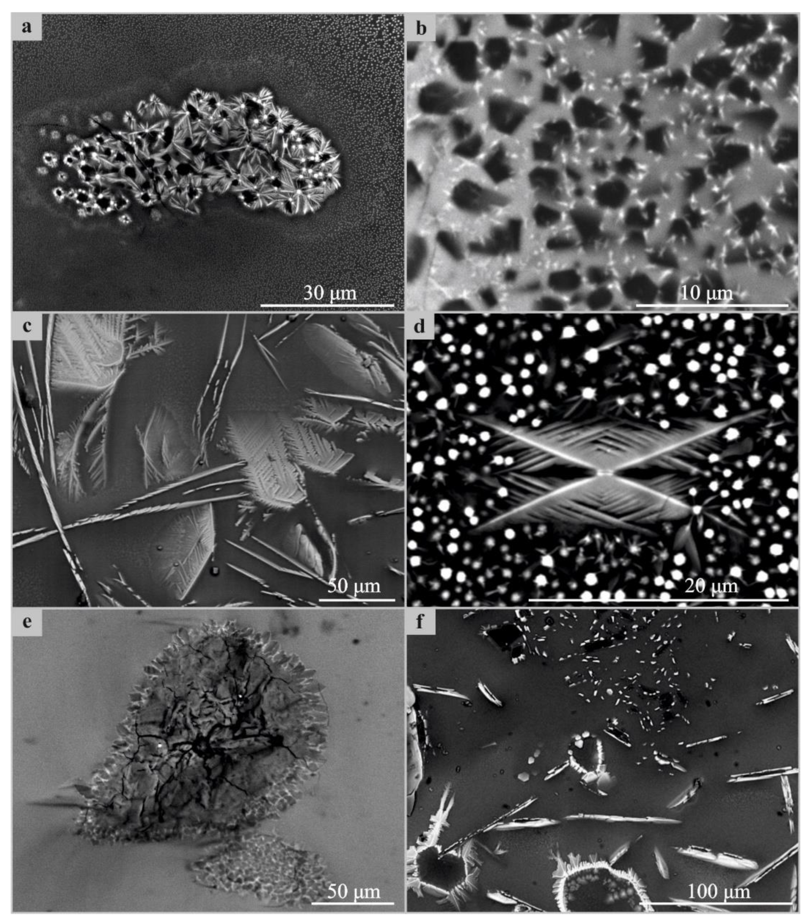
3.2. Morphology and Composition

Figure 4 shows examples of SEM images of the surfaces of the strongly magnetic samples (see Figure 2 and Table 3).

Iron oxides (hydroxides), magnetite, hematite, goethite, and others are visible on the glass surface. Morphologically, they appear as clusters of emulsion drops (a), microcrystallites (a, b), and skeletal aggregates (a, c, d, f) transforming into holohedral forms with a plate-like appearance (c, d). The plates often have hexagonal crystallographic faceting (b), from which it can be assumed that they are represented by hematite. Sometimes, there are relict areas of unmelted silica, around which microdrusy prismatic aggregates of silica (e), probably quartz, are growing. On the surface of these and in the interstices, iron oxides (hydroxides) are formed (e). The faces of earlier crystals are the intumescence surface for later ones. In comparison, the literature data on the artificial glasses obtained via the hydrothermal alteration of Martian-like synthetic basalts present a similar morphology [42]: iron mineral spherules a few micrometers in diameter. Moreover, Isobe and Yoshizawa showed the inclusions of sub-micrometer-sized iron oxide particles with the morphology of six-way petals or snowflakes [42], which can possess specific magnetic properties with several equivalent magnetic axes. Contrary to those results, Berger et al. [41] found nanosized isotropic magnesium ferrite inclusions in the glass structure, which can be superparamagnetic. Similar results regarding spherical iron oxide nanoparticles in magnetic macro/mesoporous bioglass have also been reported [36]. Additionally, the morphology of the obtained samples can be compared to the reduced basaltic glass incubated in vitro with Mariprofundus ferrooxydans, showing quite similar shapes and sizes to those of the iron oxide inclusions [31].

Figure 5, in the example of sample a¹⁰c³⁰f, shows that iron-containing particles are concentrated in the near-surface layer of the sample with a thickness of about 1–2 µm. This is confirmed by a noticeable decrease in iron content in the depth of the sample (

Table 4. Elemental content at the points of the cross section of sample a¹⁰c³⁰f (see Figure 5).

Element	Spectrum 1, wt %	Spectrum 2, wt %
O	59.84	60.73
Na	1.42	1.31
Mg	0.79	1.01
Al	5.29	5.68
Si	23.73	25.77
K	0.93	0.80
Ca	1.57	1.79
Fe	6.43	2.90

).

According to the data obtained through the XPS method (

Table 5. Results of analysis through the XPS method: binding energy (eV) and relative content (at. %) of the elements.

Sample	Na (1s)	Fe (2p3/2)	F (1s)	O (1s)		Ti (2p3/2)	Ca (2p)	C (1s)			Si (2p)	Al (2p)
a10c30f	1.0	0.7	0.3	33.7	18.1	0.3	1.7	2.0	6.0	12.1	21.9	2.2
eV	1072.9	710.9	685.5	532.8	531.4	459.8	348.0	288.0	286.0	285.0	102.7	74.2
a30c10f	0.7	0.5	–	27.3	16.1	0.1	1.5	3.2	15.4	17.1	13.2	4.8
eV	1072.9	711.0	–	533.0	531.6	459.5	348.0	288.6	286.6	285.0	102.6	74.3
sf	1.6	1.1	0.4	30.0	14.4	0.3	2.4	–	3.1	13.0	27.1	5.7
eV	1072.7	710.9	685.3	532.6	531.2	458.9	347.9	–	286.6	285.0	102.7	74.2
a30s10c5f	0.6	1.7	–	33.5	18.1	–	2.3	2.2	6.5	12.8	14.7	7.6
eV	1072.5	710.8	–	532.6	531.3	–	348.0	288.5	286.5	285.0	102.2	74.0
s10c30f	1.0	0.8	0.7	32.6	14.7	0.3	1.4	2.4	5.2	8.3	25.2	8.1
eV	1073.1	710.5	685.3	533.0	531.7	459.9	348.4	288.2	286.6	285.0	103.1	74.7
	Na+	Fe2+, Fe3+	MF	SiO2	Al2O3	Ti4+	Ca2+	OCO	COC	CC, CH	Si4+	Al3+

), the composition of the samples is dominated by oxygen, silicon, and carbon; aluminum is present in appreciable amounts. Judging by the bonding energies, O, Si, and Al are probably in the forms of SiO₂, Al₂O₃, and aluminosilicates. Carbon observed in the samples seems to be mostly introduced (adsorbed, contact). Iron observed in insignificant amounts, as far as spectra Fe (2p_3/2) allow us to judge, in the analyzed upper layers of the samples is probably strongly oxidized and is in the form of various oxides.

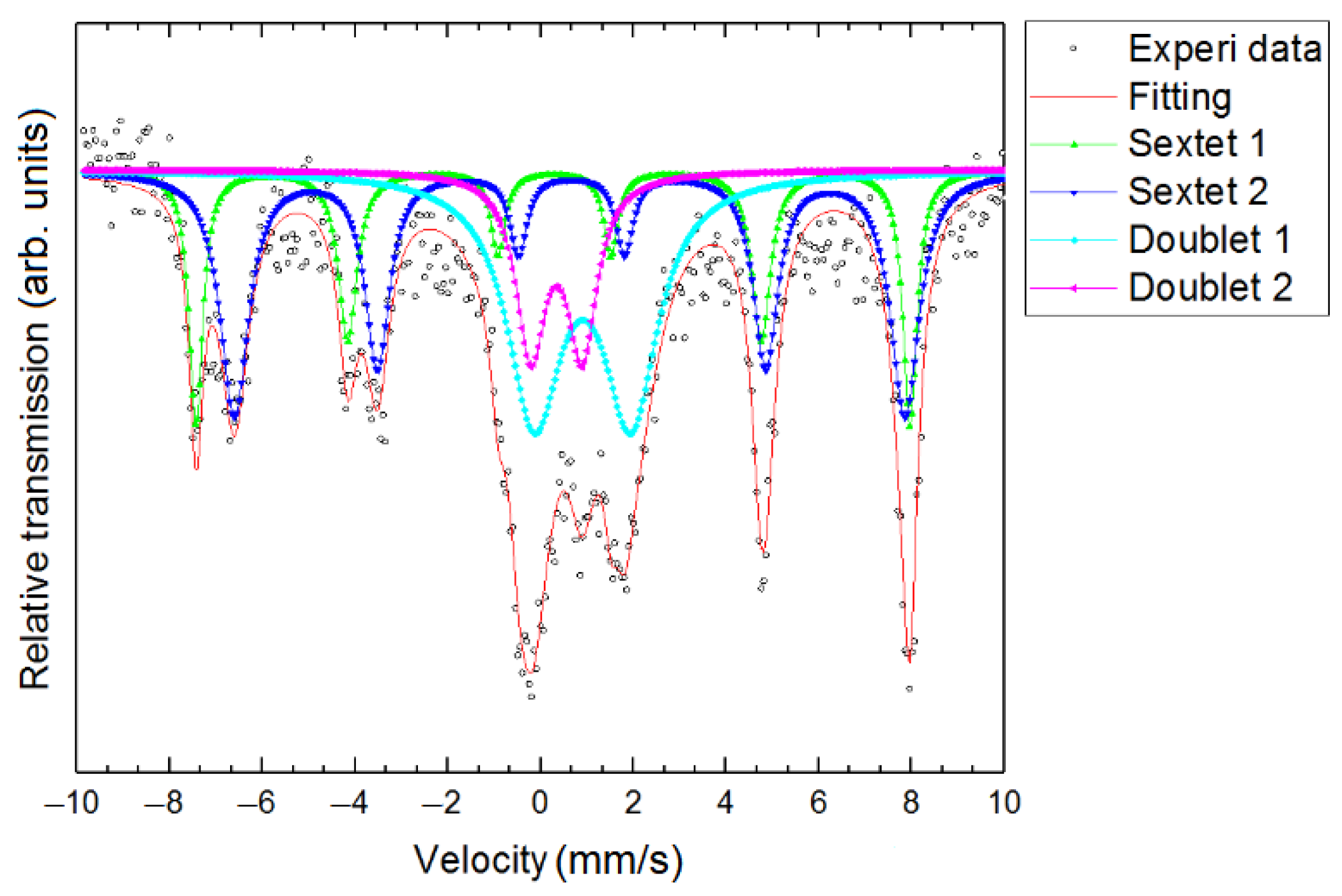
3.3. Mössbauer Spectroscopy

Figure 6 shows the Mössbauer spectrum for sample a³⁰s¹⁰f as an example (other spectra are presented in Appendix A, Figure A1). The dots show the experimental data; the bottom line corresponds to the model spectrum.

The

Table 6. Parameters of hyperfine interaction for the sample: IS—isomeric shift of the Mössbauer lines, QS—quadrupole splitting, B_Hf—effective magnetic field, S—area of lines in % of total area of the spectrum. Isomeric shifts are given relative to α-Fe.

Sample	Component	IS (mm/s)	QS (mm/s)	BHf (T)	S (%)
a10c30f	Sextet Fe(1)	0.246 ± 0.009	0.017 ± 0.018	48.454 ± 0.081	17.66
	Sextet Fe(2)	0.659 ± 0.019	0.013 ± 0.035	45.659 ± 0.143	40.39
	Doublet Fe(1)	0.863 ± 0.029	1.932 ± 0.052	–	41.95
a30c10f	Sextet Fe(1)	0.284 ± 0.008	0.032 ± 0.013	47.843 ± 0.052	20.35
	Sextet Fe(2)	0.648 ± 0.009	0.039 ± 0.016	44.925 ± 0.076	33.57
	Doublet Fe(1)	0.906 ± 0.029	2.081 ± 0.047	–	32.77
	Doublet Fe(2)	0.344 ± 0.023	1.104 ± 0.052	–	13.30
sf	Sextet Fe(1)	0.304 ± 0.000	0.064 ± 0.020	47.430 ± 0.068	20.29
	Sextet Fe(2)	0.645 ± 0.000	0.015 ± 0.028	44.209 ± 0.116	27.18
	Doublet Fe(1)	0.842 ± 0.011	2.288 ± 0.022	–	24.97
	Doublet Fe(2)	0.456 ± 0.009	0.867 ± 0.015	–	27.55
a30s10c5f	Sextet Fe(1)	0.340 ± 0.025	0.101 ± 0.047	47.337 ± 0.151	3.91
	Sextet Fe(2)	0.540 ± 0.022	0.029 ± 0.041	43.451 ± 0.220	17.09
	Doublet Fe(1)	0.872 ± 0.004	2.350 ± 0.006	–	37.51
	Doublet Fe(2)	0.463 ± 0.003	0.842 ± 0.005	–	41.49
s10c30f	Sextet Fe(1)	0.312 ± 0.020	0.060 ± 0.034	48.020 ± 0.129	17.64
	Sextet Fe(2)	0.663 ± 0.026	0.024 ± 0.043	44.869 ± 0.183	26.41
	Doublet Fe(1)	0.912 ± 0.018	2.155 ± 0.037	–	36.89
	Doublet Fe(2)	0.536 ± 0.023	0.832 ± 0.038	–	19.07

shows the parameters of hyperfine interaction for the samples under study. In all the spectra, we can distinguish sextets, the parameters of which are in good agreement with the reported values of the magnetite parameters [65], as well as doublets, which, according to our assumptions, correspond to the superparamagnetic phase.

Since all the spectra are described by a similar set of hypotheses with close values of the hyperfine interaction parameters (except for sample a¹⁰c³⁰f, which lacks the doublet corresponding to trivalent iron), we will examine only the spectrum of sample a³⁰c¹⁰f.

The spectrum has a complex structure and is best described by a combination of two doublets and two sextets. The sextets correspond to the iron atoms contained in magnetite. Sextet 1, with an isomeric shift value of 0.284 ± 0.008 mm/s and an effective field value of 47.843 ± 0.052 T, corresponds to trivalent iron atoms in the tetrahedral position, and sextet 2, with an isomeric shift value δ = 0.648 ± 0.009 mm/s and B_Hf = 44.925 ± 0.076 T, corresponds to atoms of bi- and trivalent iron, participating in the rapid electron exchange and occupying octahedral positions (of the magnetite crystal lattice).

The parameters of hyperfine interaction of doublet 1 suggest that it corresponds to the atoms of divalent iron in tetrahedral coordination, and doublet 2, in turn, corresponds to the atoms of trivalent iron in tetrahedral coordination. On the basis of the experimental and the literature data [58,66], we can assume the presence of a superparamagnetic magnetite fraction in the sample. Nevertheless, comparing to the Mössbauer spectra for the ferrosilicate glasses [40] with the only one doublet, we can state the obvious difference in the case of non-crystalline iron oxide inclusions, which can additionally confirm our current assumptions.

In samples a³⁰c¹⁰f, sf, and s¹⁰c³⁰f, the ratio of the areas of sextets S_sextet1/S_sextet2 > 0.5 (as well as the values of the hyperfine interaction parameters) indicates the presence of non-stoichiometric magnetite (for which the ratio S_sextet1/S_sextet2 = 0.5). In the spectrum of sample a¹⁰c³⁰f (S_sextet1/S_sextet2 ≈ 0.44), iron in the octahedral position predominates; however, this may be due to the “noisiness” of the spectrum due to the small iron content in the sample.

Sample a³⁰s¹⁰c⁵f somewhat stands out; in it, the magnetically ordered component in the form of two sextets with parameters close to those for magnetite, which is mainly in the superparamagnetic state, is weakly expressed.

3.4. Electron Spin Resonance

Silicate glasses, both artificial and natural, are characterized by the spectra of electron paramagnetic resonance of the X band [67], containing, as a rule, a superposition of resonance lines with g-factors >2.0, ~4.3, and, rarely, ~9.4.

The line at g~4.3 is associated with isolated tetrahedral Fe complexes in a highly rhombically distorted oxygen environment [67]. This corresponds to trivalent iron ions atomically scattered in glass in the form of an isomorphic structural impurity [68,69]. The line with g~2.0 is associated with trivalent iron clusters or oxyhydroxide inclusions (strongly and weakly magnetic, also in the superparamagnetic state). The same clusters provide the appearance of a feature on the spectrum at g~9.4, which is usually attributed to isolated Fe³⁺ ions in an axially symmetric oxygen environment. For such objects, we can speak about “ferromagnetic resonance”, distinguishing it as a special case of ESR. Such spectra of some natural glasses, for example, obsidians, may also contain resonance lines with g-factors [70]. In the spectra of artificial glasses doped with ions of various chemical elements, in particular, transition metals, there may be resonance lines with effective g-factors 4.4, 3.8, 3.1, 2.4, 2.3, and 2.0 [71].

The two types of ESR spectra were obtained on the samples under study. The first type is the closest in form to the “classical” spectra of silicate glass with a small admixture of iron ions [67,68]. Such spectra were obtained for samples a³⁰c¹⁰w, s³⁰c¹⁰w, a³⁰s¹⁰c⁵w, a¹⁰s³⁰c⁵w, s³⁰c¹⁰f, a²⁰s²⁰w, and a²⁰s²⁰f. Figure 7a shows an example of the spectrum measured at different temperatures for sample a³⁰s¹⁰c⁵w. The intense line with g = 4.24 is characterized by the fact that its width of 17 mT does not change as the temperature decreases, and the intensity increases approximately by a factor of 4 in the range of 400–100 K. The less intense and broader line g = 2.0 (99 mT and 108 mT wide at 100 and 300 K, respectively) increases in amplitude less than 1.5 times in the same temperature range. A weak line with g~9.4 is also observed. The second type of spectrum is characteristic for the case of “ferromagnetic resonance”; for example, on magnetite particles, it was obtained for samples a¹⁰c³⁰w, a³⁰c¹⁰f, s¹⁰c³⁰w, s¹⁰c³⁰f, a¹⁰s³⁰c⁵f, a³⁰s¹⁰ c⁵f, a¹⁰s³⁰c⁵f, and a¹⁰c³⁰f (Figure 7b shows the ESR spectra for sample a³⁰s¹⁰ c⁵f). The broad line with an intensity 2 orders of magnitude higher than that for the first type, with g = 2.09 at T = 300 K, shifts to the region of weak fields with g = 2.64, and has a decrease in amplitude by a factor of about 2 when the temperature changes to 100 K.

It is likely that tetrahedral Fe complexes in the paramagnetic state, scattered in the glass matrix, prevail in the samples of the first type. However, interacting octahedral Fe complexes are present in very insignificant amounts. In the samples of the second type, oxyhydroxide inclusions, particles in a superparamagnetic and low-domain state likely dominate against a background of iron ions scattered in the glass matrix (the resonance line with g~4.3, which is almost indistinguishable at 400 K, becomes brighter with decreasing temperature). This is confirmed by the fact that as the temperature decreases, the intensity of the spectrum of these samples strongly decreases, the line width increases, and the resonance field shifts in the direction of lower magnetic fields [28,70,72,73].

4. Theoretical Modeling

Five “strongly magnetic” samples were chosen for theoretical modeling, including sample s¹⁰c³⁰f from the first group (M_rs/M_s ≤ 0.1, H_cr/H_c ≥ 5), the three samples (sf, a¹⁰c³⁰f, and a³⁰c¹⁰f) from the second group (M_rs/M_s > 0.2, H_cr/H_c ≤ 5), and the intermediate (M_rs/M_s ≈ 0.18, H_cr/H_c ≈ 11) sample a³⁰s¹⁰c⁵f. All of these samples contain a sufficiently large number of SP particles, since for them, the value of fd > 1%.

A peculiarity of these glass samples is the possible relationship between chemical inhomogeneity and magnetic states; the larger the particles, the more likely they are to be oxidized from the surface (Figure 5, Table 4). As a consequence, three fractions are distinguished during modeling: (1) fairly large (PSD and possibly SD) particles subjected to oxidation; (2) smaller, stable (possibly SD and blocked SP) particles of non-stoichiometric magnetite; and (3) true SP particles. For different samples, SD particles can be both two-phase and single-phase during modeling.

Using an approximation of the lognormal distribution of particles by volume (see, for example, [74,75]), we can calculate the most probable characteristic sizes of particles in different magnetic states [63]. The probability density of the lognormal distribution is written as

$$\mathsf{\phi }(x)=\frac{1}{x\sigma \sqrt{2\mathsf{\pi }}}exp\left(-\frac{{\left(\ln (x/\alpha )\right)}^2}{2{\sigma }^2}\right),$$

(2)

where x = v/v_p is the ratio of particle volume to mean volume, σ is the standard deviation, and α is the average of the corresponding Gaussian distribution.

During modeling, four ranges of grain sizes corresponding to different magnetic states are considered: superparamagnetic (SP), stable single-domain (SD), fine pseudo-single-domain (fPSD), and coarse pseudo-single-domain (cPSD) particles, with the respective particle diameters of about 0–25, 25–40, 40–100, and 100–500 nm (see, for example, [63,76,77,78,79]). By fPSD and cPSD, we mean particles with vortex structures and a small number of domains, respectively, and we neglect the contribution of truly multidomain particles to the hysteresis characteristics.

Let us introduce relative numbers of particles corresponding to the abovementioned magnetic states: n_sp, n_ssd, n_fpsd, and n_cpsd. The relative number of particles for each group are

$$n={{\displaystyle \int }}_{x_1}^{x_2}\mathsf{\phi }(x)dx/{{\displaystyle \int }}_{x_{min}}^{x_{max}}\mathsf{\phi }(x)dx,$$

(3)

where x₁ and x₂ are the lower and upper limits of the volume range of a given particle group, respectively, and x_min (d = 0) and x_max (d = 500 nm) are the minimum and the maximum relative particle volumes, respectively, with x₂ ≤ x_max.

Previously [63], we took into consideration that the samples contained SP particles blocked by magnetostatic interaction, which can contribute not only to the saturation magnetization, but also to the remanent magnetization of the sample. Since the frequency dependence of magnetic susceptibility is due to the presence of unblocked (true) superparamagnetic particles, two groups should be distinguished: nbSP, non-blocked superparamagnetic particles (0–15 nm), and bSP, blocked superparamagnetic particles (15–25 nm) (see, for example, [80]).

It is known that the frequency-dependent susceptibility correlates with the fraction of nbSP particles in the samples, but the exact dependence of the numerical value of fd on this fraction has not yet been established [61,63]. Therefore, nbSP particle concentrations covering all fd values for the simulated samples were chosen for further calculations: 1, 2, 6, 7, and 12% (

Table 7. Fractions of the volume concentration of ferrimagnetic particles in the corresponding magnetic states; ME is the mathematical expectation of the lognormal distribution and d_mean is the mean size of ferrimagnetic particles in the sample.

Sample	Cnbsp	Cbsp	Csd	Cfpsd	Ccpsd	ME	dmean, nm
a30c10f	0.010	0.075	0.233	0.656	0.026	5.35	33.6
a10c30f	0.020	0.097	0.237	0.619	0.027	3.79	29.7
sf	0.060	0.136	0.233	0.543	0.028	1.34	20.5
s10c30f	0.070	0.142	0.231	0.530	0.027	1.05	18.9
a30s10c5f	0.120	0.158	0.218	0.477	0.027	0.31	12.3

). The desired concentrations were achieved by selecting the mathematical expectation (ME) of the lognormal distribution with a fixed standard deviation SQ = 20.

The relative number of nbSP particles is obtained using Equation (3) when x₁ = 0 and x₂ = x_bsp (the volume corresponding to the blocking size; in our case, d_bsp = 15 nm). Then the relative average volume of nbSP particles is:

$$x_{nbsp}={\displaystyle \underset{0}{\overset{x_{bsp}}{\int }}x\mathsf{\phi }(x)dx}.$$

(4)

Similarly, it is possible to calculate the relative average volumes of other groups of particles in different magnetic states. In this case, the average volume and size of ferrimagnetic particles in the sample can be calculated by the formulas:

$$v_{mean}=v_p\cdot \left(n_{nbsp}{x}_{nbsp}+n_{bsp}{x}_{bsp}+n_{sd}{x}_{sd}+n_{fpsd}{x}_{fpsd}+n_{cpsd}{x}_{cpsd}\right),$$

$$d_{mean}={\left(6v_{mean}/\mathsf{\pi }\right)}^{1/3}.$$

(5)

Then, the fraction of volume concentration of non-blocked ferrimagnetic particles in the sample is

$$C_{nbsp}=n_{nbsp}\frac{v_{nbsp}}{v_{mean}},\mathrm{where}{v}_{nbsp}=v_p{x}_{nbsp},$$

(6)

and the sum of fractions for all the groups of particles is equal to one.

The best results for different C_nbsp values (consistent with the experimental values of M_rs, M_s, H_cr, and H_c) were obtained using the characteristic size of ferrimagnetic particles, d_p = 20 nm, and the volume of spherical particles, v_p = (π/6)·d_p³, corresponding to it.

Two models were used in further calculations: the model of chemically inhomogeneous two-phase particles (TPh model) [58,81,82] and the model of single-domain particles with effective spontaneous magnetization (SDEM model) [83,84,85]. It is known that, at sufficiently large concentrations of the ferrimagnet, magnetization of the sample is significantly affected by magnetostatic interaction between the ferrimagnetic particles, which was taken into consideration in the both models.

In the TPh model, an ensemble of cubic two-phase particles was considered with the characteristic particle size a and the phase volumes (1 − ε)a³—the strongly magnetic phase (magnetite)—and εa³—the weakly magnetic phase (hematite). It was assumed that the light magnetization axes of the phases are parallel to the interphase boundary. Then, in the absence of an external field, the magnetic moments in the phases are either opposite in direction or their directions coincide. Applying an external field along the light axes does not increase the number of possible states of a particle, but changes the values of their relative fraction. The number of particles in different states was calculated on the basis of the statistical Boltzmann distribution. This allowed calculating the particle magnetization reversal fields and estimating the hysteresis characteristics of the sample. The sample magnetization in field H was calculated in the approximation of a uniform distribution of random interaction fields H_i in the range from −H_max to +H_max:

$$M\left(H\right)=\frac{1}{2H_{max}}\underset{-H_{max}}{\overset{H_{max}}{{\displaystyle \int }}}M(H,H_i)d{H}_i$$

(7)

Here, M (H, H_i) is determined by the number of particles in different magnetic states. Then, the magnetization calculation is reduced to the case of non-interacting particles, taking into consideration the reduction in the critical fields by the value of H_max.

Using the SDEM model, in the mean-field approximation, we can more rigorously account for the influence of magnetostatic interaction, compared to the case of the uniform distribution function H_i, and obtain the random-field distribution functions for any bulk concentrations of the ferrimagnet [86]. Then, using the experimental values of magnetizations (M_s, M_rs) and coercive forces (H_c, H_cr), we can calculate the effective spontaneous magnetizations of the particles by saturation, I_{s eff}, and by saturation remanence, I_{rs eff}. The introduction of effective spontaneous magnetizations enables estimating the influence of magnetic moment inhomogeneity in the volume of a particle, which is determined by the formation of domain and vortex structures, as well as by possible chemical inhomogeneity [56,87,88].

To find the I_{s eff} and I_{rs eff} magnetizations, we solved the inverse problem of matching the theoretical values of these magnetizations, calculated by both of the models, with the experimental data. The dimensionless magnetization ζ and the volumetric concentration C_f of the ferrimagnetic particles involved in its formation were used in the calculations:

$$\mathsf{\zeta }=\frac{M}{C_f{I}_{eff}},C_f=N\frac{v_{mean}}{V_s}.$$

(8)

Here, M stands for M_s or M_rs and N is the number of particles with mean volume v_mean and concentration C_f in the sample of volume V_s. The value of magnetization of a system of uniaxial ferrimagnetic particles randomly distributed in a cylindrical volume is determined by the modified method of moments and expansion into a Gram–Charlier series [84,86].

In classic works [89,90], the analogy of spin glasses and objects of rock magnetism was used. If we consider spin clusters to be magnetic moments of particles in rock magnetism, we can use the ideas related to superparamagnetism and study the dependence of the conditions of the blocking of magnetic moments on various parameters. For example, in [90], the blocking temperature was studied. In our models, the temperature is fixed. We consider the dependence of the blocking volume of the SP particle on the total field using particle H + H_i and its magnetization reversal field, H₀.

As indicated above, the interaction leads to the blocking of the magnetic moments of the SP particles, which contribute to the remanent magnetization. For the blocked particles, the time-averaged non-zero magnetic moment is (see, for example, [58]):

$$m\left(v,H_i\right)=v{I}_s\tanh \left(\frac{v_b\left(H_i\right)I_s\left|H+H_i\right|}{kT}\right)=v{I}_{rs eff},$$

(9)

where I_s is the spontaneous magnetization of the ferrimagnet at temperature T and v_b(H_i) is the critical volume of the particle, the magnetic moment of which remains stable when interaction field H_i acts on the particle. In this case, the blocking volume is

$$v_b\left(H_i\right)=\{\begin{array}{c}{v}_b/{\left(1+\frac{\left|H+H_i\right|}{H_0}\right)}^2,\left|H+H_i\right|\le H_0;\\ v_b/\left(\frac{4\left|H+H_i\right|}{H_0}\right),\left|H+H_i\right|>H_0.\end{array}$$

(10)

The magnetization reversal field H₀ ≈ H_cr and v_b ≈ 50kT/(I_sH₀) is the blocking volume at H_i = 0 [91].

Since we distinguish three fractions in the samples (larger oxidized, small chemically homogeneous, and true superparamagnetic particles), the saturation magnetizations of the samples are

$$M_s=M_{s1}+M_{s2}+M_{ssp}, M_{rs}=M_{rs1}+M_{rs2}.$$

(11)

Moreover, the experimental values of M_s and M_rs agree with the results of calculations through the TPh and SDEM models:

$$M_s=C_f{I}_{seff}, M_{rs}=C_f(1-C_{nbsp})I_{rseff}.$$

(12)

The theoretical values of the magnetization reversal fields H₀ of the fraction of chemically inhomogeneous particles were calculated using the TPh model [58,82]. To estimate the theoretical H₀ values of fractions containing chemically homogeneous particles, approximations were used:

(1) For SD particles,

$$H_{0sd}=\frac{2K_u}{I_s},$$

(13)

where K_u is the constant of uniaxial crystallographic anisotropy;

(2) For bSP particles [92],

$$H_{0bsp}=H_{0sd}\left\{1-{\left[v_b\left(H_i\right)/v\right]}^{1/2}\right\},$$

(14)

where the value of v lies in the range from v_b (without regard to the interaction) to the critical volume of the single-domain particle.

The experimental values of H_cr can be coordinated with the results of calculations according to the applied models as follows:

(1) For the samples in which SD particles are chemically homogeneous and are part of the first fraction,

$$H_{02}=H_{0bsp} , H_{01}=\frac{H_{cr}\cdot \left(C_{bsp}+C_{sd}+C_{psd}\right)-H_{02}{C}_{bsp}}{C_{sd}+C_{psd}},$$

(15)

(2) For the samples in which SD particles are chemically inhomogeneous and are part of the second fraction,

$$H_{02}=\frac{H_{0sd}{C}_{sd}+H_{0bsp}{C}_{bsp}}{C_{sd}+C_{bsp}},H_{01}=\frac{H_{cr}\cdot \left(C_{bsp}+C_{sd}+C_{psd}\right)-H_{02}\cdot \left(C_{bsp}+C_{sd}\right)}{C_{psd}}.$$

(16)

Then, the theoretical values of H_c are approximately equal to the experimental values, since H₀ ≈ H_cr.

The following values of spontaneous magnetizations were used during modeling, taking into consideration possible non-stoichiometry of the material: magnetite I_s = (450–480)·10³ A/m and hematite I_s = (1–3)·10³ A/m [93,94,95]. The calculations according to the two models were performed for different values of the thickness of the weakly magnetic (hematite) phase ε in the range from 0 to 1 with a step of 0.05, taking into consideration the assumed fraction of nbSP particles (see Table 3 and Table 7). After calculating the magnetization-reversal fields of the fraction of chemically inhomogeneous particles (TPh model) and estimating the magnetization-reversal fields of the fraction of chemically homogeneous particles (Equations (13)–(16)), the effective spontaneous magnetizations I_{s eff} and I_{rs eff} (SDEM model) were calculated in agreement with the experimental data. Each sample was modeled assuming the equality of fd and the nbSP particle concentration. The results are presented in

Table 8. The results of coordinated modeling (TPh and SDEM models) of the “strongly magnetized” samples. The contributions of the three considered fractions to magnetizations M_s and M_rs. The volume concentrations of ferrimagnetic C_f in the samples and the corresponding effective spontaneous magnetizations, I_{s eff} and I_{rs eff}, are given.

No.	Sample	ε	Cf, 10–3	Ms = Ms1 + Ms2 + Ms sp, A·m2/kg		Mrs = Mrs1 + Mrs2, A·m2/kg		Is eff, kA/m	Irs eff, kA/m
1	a10c30f	0.05	9	2.96	1.88 + 1.02 + 0.06	1.14	0.73 + 0.41	465	286
2	a30c10f	0.85	20	3.02	0.75 + 2.20 + 0.07	1.15	0.28 + 0.87	203	167
3	sf	0.05	14	4.60	2.57 + 1.75 + 0.28	1.30	0.76 + 0.54	466	266
4	a30s10c5f	0.90	4	0.70	0.07 + 0.48 + 0.15	0.12	0.01 + 0.11	263	110
5	s10c30f	0.75	10	1.39	0.67 + 0.48 + 0.24	0.5 × 10–3	(0.3 + 0.2) × 10–3	198	~1

.

The best agreement with the experimental data was obtained at a large oxidation degree ε for the most highly coercive samples (a³⁰c¹⁰f and a³⁰s¹⁰c⁵f), and at small ε for the samples with lower coercivity (a¹⁰c³⁰f and sf). Additionally, in the abovementioned four samples during modeling, the SD particles belonged to the second (magnetite) fraction. For the low-coercivity sample s¹⁰c³⁰f with very low remanent magnetization, SD particles belonged to the first fraction (magnetite–hematite), with a large fraction of hematite.

In all the samples, the ferrimagnetic volume concentration is small and is in the range of (4–20) × 10^–3. For the samples with large values of ε, the value of I_{s eff} turns out to be significantly smaller than that of the spontaneous magnetization of magnetite due to chemical inhomogeneity. In all the samples, I_{rs eff} decreases compared to I_{s eff} due to the deviation of magnetic moments in the zero external field to chaotically distributed easy axes, as well as due to the manifestation of magnetic inhomogeneity in PSD particles (appearance of domain and vortex structures) and unblocking of a part of bSP particles.

5. Conclusions

Artificial glasses containing micro- and nanoparticles of iron oxides and hydroxides in various magnetic states were obtained through the method of high-temperature melting of rocks.

The main factors affecting the magnetic properties of glasses and the fraction of magnetic phase in them are the conditions of the melt cooling. In the case of rapid cooling, the iron component is tetrahedral complexes of Fe dispersed in the glass matrix, interacting octahedral complexes of Fe, and particles in the superparamagnetic state. The samples that cool down slowly also contain iron oxide particles in different magnetic states, from superparamagnetic to multidomain.

The magnetic properties of glasses are also influenced by the composition of the initial charge. Samples with the highest content of highly coercive volcanogenic–sedimentary rock also exhibit highly coercive properties.

The highest concentration of the strongly magnetic iron component is on the surface of the samples. When the melt cools down, a layer formed by iron oxide grains appears at the boundary with air.

The comparison with the literature data on the experimental studies of the artificial glasses with the inclusions of iron oxide atomic clusters and nano- and microsized particles showed the similarity in the part of surface morphology (the shape and the size of the iron oxide particles) and in the part of magnetic properties (the saturation mass magnetization and the coercivity). At the same time, there is no detailed investigation of magnetic granulometry, electron spin resonance, or theoretical modeling of magnetic states in the previous studies on artificial glasses; therefore, the current study can add original and new information to the field.

When modeling the hysteresis characteristics of the strongly magnetic samples of artificial glasses, we demonstrated coordinated applicability of the two theoretical models (TPh and SDEM) that take into consideration the magnetostatic interaction between ferrimagnetic particles. The TPh model allows taking into consideration the chemical inhomogeneity of the particle and the magnetostatic interaction between phases, as well as calculating the magnetization-reversal fields of the particle and the number of particles in the different magnetic states. The advantage of the SDEM model is a more rigorous consideration of magnetostatic interaction at any concentrations of ferrimagnetic particles. Both the models can be applied not only to the samples containing mainly single-domain and low-domain chemically inhomogeneous ferrimagnetic particles, but also to the samples containing a large number of superparamagnetic particles, including those blocked due to magnetostatic interaction.

The experimental results obtained with the use of magnetic granulometry and frequency-field dependencies of magnetic susceptibility of the samples allowed us to assume the presence of a significant number of superparamagnetic particles with a relatively small content of the ferrimagnetic component in the samples. Theoretical calculations confirmed this assumption and allowed estimating the content of both the true superparamagnetic fraction (volume concentration~10^–4) and the particles blocked due to magnetostatic interaction (volume concentration~10^–3) in the samples.

References

1. Dressler, B.O.; Reimold, W.U. Terrestrial impact melt rocks and glasses. Earth-Science Rev. 2001, 56, 205–284. [Google Scholar] [CrossRef]
2. De Graaff, S.J.; Kaskes, P.; Déhais, T.; Goderis, S.; Debaille, V.; Ross, C.H.; Gulick, S.P.S.; Feignon, J.G.; Ferrière, L.; Koeberl, C.; et al. New insights into the formation and emplacement of impact melt rocks within the Chicxulub impact structure, following the 2016 IODP-ICDP Expedition 364. Bull. Geol. Soc. Am. 2022, 134, 293–315. [Google Scholar] [CrossRef]
3. Feignon, J.G.; Schulz, T.; Ferrière, L.; Goderis, S.; de Graaff, S.J.; Kaskes, P.; Déhais, T.; Claeys, P.; Koeberl, C. Search for a meteoritic component within the impact melt rocks of the Chicxulub impact structure peak ring, Mexico. Geochim. Cosmochim. Acta 2022, 323, 74–101. [Google Scholar] [CrossRef]
4. Bogatikov, O.A.; Petrov, O.V.; Sharpenok, L.N. Petrographic Code of Russia. Igneous, Metamorphic, Metasomatic, Impact Formations; Russian Geological Research Institute: Saint Petersburg, Russia, 2008; ISBN 9785937611062. (In Russian) [Google Scholar]
5. Melosh, H.J. Impact Cratering: A Geologic Process; Oxford University Press: Oxford, UK, 1996; ISBN 0195104633. [Google Scholar]
6. Batanova, A.M.; Gramenitsky, E.N.; Kotelnikov, A.R.; Plechov, P.Y.; Shchekina, T.I. Experimental and Technical Petrology; Scientific World: Moscow, Russia, 2000; ISBN 5891761203. (In Russian) [Google Scholar]
7. Duchkov, A.D. Laboratory modeling of hydrate formation in rock specimens (a review). Russ. Geol. Geophys. 2017, 58, 240–252. [Google Scholar] [CrossRef]
8. Wawrzyniak-Guz, K. Rock physics modelling for determination of effective elastic properties of the lower Paleozoic shale formation, North Poland. Acta Geophys. 2019, 67, 1967–1989. [Google Scholar] [CrossRef]
9. Okunevich, V.S.; Bayuk, I.O. Petrophysical modeling of rocks dominik formation as the basis of interpretation of seismic data. Mosc. Univ. Bull. Ser. 4 Geol. 2022, 4, 149–156. [Google Scholar] [CrossRef]
10. Fomichev, S.V.; Babievskaya, I.Z.; Dergacheva, N.P.; Noskova, O.A.; Krenev, V.A. Criteria for assessing technological properties of gabbro-basalt rocks. Theor. Found. Chem. Eng. 2012, 46, 424–428. [Google Scholar] [CrossRef]
11. Krenev, V.A.; Pechenkina, E.N.; Fomichev, S.V. Gabbro–Basalt Raw Materials of Russia: Mineral Composition, Modification Methods, and Complex Use. Russ. J. Inorg. Chem. 2021, 66, 253–257. [Google Scholar] [CrossRef]
12. Khater, G.A.; Abdel-Motelib, A.; El Manawi, A.W.; Abu Safiah, M.O. Glass-ceramics materials from basaltic rocks and some industrial waste. J. Non. Cryst. Solids 2012, 358, 1128–1134. [Google Scholar] [CrossRef]
13. Khater, G.A.; Mahmoud, M.A. Preparation and characterization of nucleated glass-ceramics based on basaltic rocks. J. Aust. Ceram. Soc. 2017, 53, 433–441. [Google Scholar] [CrossRef]
14. Kizilkanat, A.B.; Kabay, N.; Akyüncü, V.; Chowdhury, S.; Akça, A.H. Mechanical properties and fracture behavior of basalt and glass fiber reinforced concrete: An experimental study. Constr. Build. Mater. 2015, 100, 218–224. [Google Scholar] [CrossRef]
15. Simon, S.; Prathap, A.; Balki, S.; Dhilip Kumar, R.G. An experimental investigation on concrete with basalt rock fibers. J. Phys. Conf. Ser. IOP 2021, 2070, 012196. [Google Scholar] [CrossRef]
16. Deák, T.; Czigány, T. Chemical Composition and Mechanical Properties of Basalt and Glass Fibers: A Comparison. Text. Res. J. 2009, 79, 645–651. [Google Scholar] [CrossRef]
17. Hausrath, R.L.; Longobardo, A.V. High-strength glass fibers and markets. In Fiberglass and Glass Technology: Energy-Friendly Compositions and Applications; Springer Science & Business Media: Berlin/Heidelberg, Germany, 2010; pp. 197–225. ISBN 9781441907356. [Google Scholar]
18. Höland, W.; Beall, G.H. Glass-Ceramic Technology; John Wiley & Sons: Hoboken, NJ, USA, 2012. [Google Scholar]
19. Acar, V.; Cakir, F.; Alyamaç, E.; Seydibeyoğlu, M.Ö. Basalt fibers. In Fiber Technology for Fiber-Reinforced Composites; Elsevier: Amsterdam, The Netherlands, 2017; pp. 169–185. ISBN 9780081009932. [Google Scholar]
20. Bretcanu, O.; Spriano, S.; Verné, E.; Cöisson, M.; Tiberto, P.; Allia, P. The influence of crystallised Fe3O4 on the magnetic properties of coprecipitation-derived ferrimagnetic glass-ceramics. Acta Biomater. 2005, 1, 421–429. [Google Scholar] [CrossRef] [PubMed]
21. Zaitsev, D.D.; Gravchikova, E.A.; Kazin, P.E.; Garshev, A.V.; Tret’yakov, Y.D.; Jansen, M. Preparation of magnetic glass-ceramics through glass crystallization in the Na2O-SrO-Fe2O3-B2O3 system. Inorg. Mater. 2006, 42, 326–330. [Google Scholar] [CrossRef]
22. Kushnir, S.E.; Vasil’Ev, A.V.; Zaitsev, D.D.; Kazin, P.E.; Tret’Yakov, Y.D. Synthesis of magnetoresistive glass-ceramic composites in the SrO-MnOx-SiO2-La2O3 system. J. Surf. Investig. 2008, 2, 34–36. [Google Scholar]
23. Gubin, S.P.; Koksharov, Y.A.; Khomutov, G.B.; Yurkov, G.Y. Magnetic nanoparticles: Preparation, structure and properties. Usp. Khim. 2005, 74, 539–574. [Google Scholar] [CrossRef]
24. Pomogailo, A.D.; Rozenberg, A.S.; Uflyand, I.E. Metal Nanoparticles in Polymers; Chemistry: Moscow, Russia, 2000; ISBN 5-7245-1107-X. (In Russian) [Google Scholar]
25. Heilmann, A. Polymer Films with Embedded Metal Nanoparticles; Springer Science & Business Media: Berlin/Heidelberg, Germany, 2003; ISBN 978-3-662-05233-4. [Google Scholar] [CrossRef]
26. Sunil, D.; Sokolov, J.; Rafailovich, M.H.; Duan, X.; Gafney, H.D. Evidence for the Photodeposition of Elemental Iron in Porous Vycor Glass. Inorg. Chem. 1993, 32, 4489–4490. [Google Scholar] [CrossRef]
27. Roy, S.; Roy, B.; Chakravorty, D. Magnetic properties of iron nanoparticles grown in a glass matrix. J. Appl. Phys. 1996, 79, 1642–1645. [Google Scholar] [CrossRef]
28. Berger, R.; Bissey, J.C.; Kliava, J.; Daubric, H.; Estournès, C. Temperature dependence of superparamagnetic resonance of iron oxide nanoparticles. J. Magn. Magn. Mater. 2001, 234, 535–544. [Google Scholar] [CrossRef]
29. Berger, R.; Kliava, J.; Bissey, J.C.; Baïetto, V. Magnetic resonance of superparamagnetic iron-containing nanoparticles in annealed glass. J. Appl. Phys. 2000, 87, 7389–7396. [Google Scholar] [CrossRef]
30. Godsell, J.F.; Donegan, K.P.; Tobin, J.M.; Copley, M.P.; Rhen, F.M.F.; Otway, D.J.; Morris, M.A.; O’Donnell, T.; Holmes, J.D.; Roy, S. Magnetic properties of Ni nanoparticles on microporous silica spheres. J. Magn. Magn. Mater. 2010, 322, 1269–1274. [Google Scholar] [CrossRef]
31. Henri, P.A.; Rommevaux-Jestin, C.; Lesongeur, F.; Mumford, A.; Emerson, D.; Godfroy, A.; Ménez, B. Structural iron (II) of basaltic glass as an energy source for zetaproteobacteria in an abyssal plain environment, off the mid-Atlantic ridge. Front. Microbiol. 2016, 6, 1518. [Google Scholar] [CrossRef]
32. Kursawe, M.; Anselmann, R.; Hilarius, V.; Pfaff, G. Nano-particles by wet chemical processing in commercial applications. J. Sol-Gel Sci. Technol. 2005, 33, 71–74. [Google Scholar] [CrossRef]
33. Wang, C.H.; Lin, X.C.; Yang, S.S.; Liu, S.Q.; Yoon, S.; Wang, Y.G. Evaluation of the thermal and rheological characteristics of minerals in coal using SiO2-Al2O3-CaO-FeOx quaternary system. Ranliao Huaxue Xuebao/J. Fuel Chem. Technol. 2016, 44, 1025–1033. [Google Scholar] [CrossRef]
34. Senanayake, G.; Das, G.K. A comparative study of leaching kinetics of limonitic laterite and synthetic iron oxides in sulfuric acid containing sulfur dioxide. Hydrometallurgy 2004, 72, 59–72. [Google Scholar] [CrossRef]
35. Baikousi, M.; Agathopoulos, S.; Panagiotopoulos, I.; Georgoulis, A.D.; Louloudi, M.; Karakassides, M.A. Synthesis and characterization of sol-gel derived bioactive CaO-SiO2-P2O5 glasses containing magnetic nanoparticles. J. Sol-Gel Sci. Technol. 2008, 47, 95–101. [Google Scholar] [CrossRef]
36. Wang, D.; Lin, H.; Jiang, J.; Han, X.; Guo, W.; Wu, X.; Jin, Y.; Qu, F. One-pot synthesis of magnetic, macro/mesoporous bioactive glasses for bone tissue engineering. Sci. Technol. Adv. Mater. 2013, 14, 25004. [Google Scholar] [CrossRef]
37. Shahar, A.; Hillgren, V.J.; Horan, M.F.; Mesa-Garcia, J.; Kaufman, L.A.; Mock, T.D. Sulfur-controlled iron isotope fractionation experiments of core formation in planetary bodies. Geochim. Cosmochim. Acta 2015, 150, 253–264. [Google Scholar] [CrossRef]
38. Ahmadzadeh, M.; Marcial, J.; McCloy, J. Crystallization of iron-containing sodium aluminosilicate glasses in the NaAlSiO4-NaFeSiO4 join. J. Geophys. Res. Solid Earth 2017, 122, 2504–2524. [Google Scholar] [CrossRef]
39. Abdallah, E.A.M.; Gagnon, G.A. Arsenic removal from groundwater through iron oxyhydroxide coated waste products. Can. J. Civ. Eng. 2009, 36, 881–888. [Google Scholar] [CrossRef]
40. Jackson, W.E.; Farges, F.; Yeager, M.; Mabrouk, P.A.; Rossano, S.; Waychunas, G.A.; Solomon, E.I.; Brown, G.E. Multi-spectroscopic study of Fe(II) in silicate glasses: Implications for the coordination environment of Fe(II) in silicate melts. Geochim. Cosmochim. Acta 2005, 69, 4315–4332. [Google Scholar] [CrossRef]
41. Berger, G.; Cathala, A.; Fabre, S.; Borisova, A.Y.; Pages, A.; Aigouy, T.; Esvan, J.; Pinet, P. Experimental exploration of volcanic rocks-atmosphere interaction under Venus surface conditions. Icarus 2019, 329, 8–23. [Google Scholar] [CrossRef]
42. Isobe, H.; Yoshizawa, M. Formation of iron mineral fine particles by acidic hydrothermal alteration experiments of synthetic martian basalt. J. Mineral. Petrol. Sci. 2014, 109, 62–73. [Google Scholar] [CrossRef]
43. Ward, C.R.; French, D. Determination of glass content and estimation of glass composition in fly ash using quantitative X-ray diffractometry. Fuel 2006, 85, 2268–2277. [Google Scholar] [CrossRef]
44. Dyadenko, M.V.; Levitskii, I.A.; Sidorevich, A.G. Influence of the Structure of the Glasses from the BaO–La2O3–B2O3–ZrO2–TiO2–SiO2–Nb2O5 System on Their Thermal Expansion and Technological Characteristics. Glas. Phys. Chem. 2022, 48, 341–350. [Google Scholar] [CrossRef]
45. Rietveld, H.M. A profile refinement method for nuclear and magnetic structures. J. Appl. Crystallogr. 1969, 2, 65–71. [Google Scholar] [CrossRef]
46. Masaitis, V.L.; Danilin, A.N.; Mashchak, M.S.; Raikhlin, A.I.; Selivanovskaia, T.V.; Shadenkov, E.M. The Geology of Astroblemes; Nedra: Leningrad, Russia, 1980. (In Russian) [Google Scholar]
47. Ubbelohde, A.R. Melting and crystal structure. Q. Rev. Chem. Soc. 1950, 4, 356–381. [Google Scholar] [CrossRef]
48. Ubbelohde, A.R. Melting and Crystal Structure—Some Current Problems. Angew. Chem. Int. Ed. Engl. 1965, 4, 587–591. [Google Scholar] [CrossRef]
49. Sobolev, R.N. The temperature range of melting of crystalline material. Dokl. Earth Sci. 2017, 473, 367–370. [Google Scholar] [CrossRef]
50. Sobolev, R.N.; Mal’tsev, V.V.; Volkova, E.A. Experimental Investigation of the Melting of Minerals and Rocks. Russ. Metall. 2021, 2021, 102–108. [Google Scholar] [CrossRef]
51. Masaitis, V.L. Structures and Textures of Explosive Breccias and Impactites; Nedra: Leningrad, Russia, 1983. (In Russian) [Google Scholar]
52. Torre, E. Della Magnetic Hysteresis; Wiley-IEEE Press: Hoboken, NJ, USA, 2000; ISBN 9780470545195. [Google Scholar]
53. Altshuler, S.A.; Kozyrev, B.M. Electron Paramagnetic Resonance in Compounds of Transition Elements; John Wiley & Sons: New York, NJ, USA, 1974; ISBN 978-0-470-02523-9. [Google Scholar]
54. Day, R.; Fuller, M.; Schmidt, V.A. Hysteresis properties of titanomagnetites: Grain-size and compositional dependence. Phys. Earth Planet. Inter. 1977, 13, 260–267. [Google Scholar] [CrossRef]
55. Dunlop, D.J. Theory and application of the Day plot (Mrs/Ms versus Hcr/Hc) 2. Application to data for rocks, sediments, and soils. J. Geophys. Res. 2002, 107, EPM 5-1–EPM 5-15. [Google Scholar] [CrossRef]
56. Roberts, A.P.; Tauxe, L.; Heslop, D.; Zhao, X.; Jiang, Z. A Critical Appraisal of the “Day” Diagram. J. Geophys. Res. Solid Earth 2018, 123, 2618–2644. [Google Scholar] [CrossRef]
57. Ralin, A.Y.; Kharitonskii, P.V. Effect of thermal fluctuations on the stability of the magnetic state of small two-phase ferrimagnetic particles. Phys. Met. Metallogr. 2002, 93, 109–114. [Google Scholar]
58. Kharitonskii, P.; Zolotov, N.; Kirillova, S.; Gareev, K.; Kosterov, A.; Sergienko, E.; Yanson, S.; Ustinov, A.; Ralin, A. Magnetic granulometry, Mössbauer spectroscopy, and theoretical modeling of magnetic states of FemOn–Fem-xTixOn composites. Chin. J. Phys. 2022, 78, 271–296. [Google Scholar] [CrossRef]
59. Kirshvink, J.L. (Ed.) Magnetite Biomineralization and Magnetoreception in Organisms. A New Biomagnetism; Plenum Press: New York, NY, USA, 1985. [Google Scholar]
60. Eyre, J.K. Frequency dependence of magnetic susceptibility for populations of single-domain grains. Geophys. J. Int. 1997, 129, 209–211. [Google Scholar] [CrossRef]
61. Egli, R. Magnetic susceptibility measurements as a function of temperature and frequency I: Inversion theory. Geophys. J. Int. 2009, 177, 395–420. [Google Scholar] [CrossRef]
62. Hrouda, F. Models of frequency-dependent susceptibility of rocks and soils revisited and broadened. Geophys. J. Int. 2011, 187, 1259–1269. [Google Scholar] [CrossRef]
63. Kharitonskii, P.; Bobrov, N.; Gareev, K.; Kosterov, A.; Nikitin, A.; Ralin, A.; Sergienko, E.; Testov, O.; Ustinov, A.; Zolotov, N. Magnetic granulometry, frequency-dependent susceptibility and magnetic states of particles of magnetite ore from the Kovdor deposit. J. Magn. Magn. Mater. 2022, 553, 169279. [Google Scholar] [CrossRef]
64. Dearing, J.A.; Dann, R.J.L.; Hay, K.; Lees, J.A.; Loveland, P.J.; Maher, B.A.; O’Grady, K. Frequency-dependent susceptibility measurements of environmental materials. Geophys. J. Int. 1996, 124, 228–240. [Google Scholar] [CrossRef]
65. Gotić, M.; Musić, S. Mössbauer, FT-IR and FE SEM investigation of iron oxides precipitated from FeSO4 solutions. J. Mol. Struct. 2007, 834–836, 445–453. [Google Scholar] [CrossRef]
66. Kharitonskii, P.; Kamzin, A.; Gareev, K.; Valiullin, A.; Vezo, O.; Sergienko, E.; Korolev, D.; Kosterov, A.; Lebedev, S.; Gurylev, A.; et al. Magnetic granulometry and Mössbauer spectroscopy of FemOn–SiO2 colloidal nanoparticles. J. Magn. Magn. Mater. 2018, 461, 30–36. [Google Scholar] [CrossRef]
67. Castner, T.; Newell, G.S.; Holton, W.C.; Slighter, C.P. Note on the paramagnetic resonance of iron in glass. J. Chem. Phys. 1960, 32, 668–673. [Google Scholar] [CrossRef]
68. Antoni, E.; Montagne, L.; Daviero, S.; Palavit, G.; Bernard, J.L.; Wattiaux, A.; Vezin, H. Structural characterization of iron-alumino-silicate glasses. J. Non-Cryst. Solids 2004, 345–346, 66–69. [Google Scholar] [CrossRef]
69. Lyutoev, V.P.; Lysiuk, A.Y.; Karlova, L.O.; Beznosikov, D.S.; Zhuk, N.A. ESR and 57Fe Mössbauer Spectroscopy Study of Fe-doped SrBi2Nb2O9. J. Sib. Fed. Univ.—Math. Phys. 2022, 15, 450–458. [Google Scholar] [CrossRef]
70. Griscom, D.L. Ferromagnetic resonance of precipitated phases in natural glasses. J. Non. Cryst. Solids 1984, 67, 81–118. [Google Scholar] [CrossRef]
71. Radchenko, Y.S.; Levitskii, I.A.; Ugolev, I.I. Investigation of glasses and glaze coats of composition R2O-RO-Fe2O3(FeO)-Al2O3-B2O3-SiO2 by the EPR method. J. Appl. Spectrosc. 2003, 70, 821–826. [Google Scholar] [CrossRef]
72. Griscom, D.L. Electron spin resonance in glasses. J. Non. Cryst. Solids 1980, 40, 211–272. [Google Scholar] [CrossRef]
73. Bodziony, T.; Guskos, N.; Typek, J.; Roslaniec, Z.; Narkiewicz, U.; Kwiatkowska, M.; Maryniak, M. Temperature dependence of the FMR spectra of Fe3O4 and Fe3C nanoparticle magnetic systems in copolymer matrices. Mater. Sci. Pol. 2005, 23, 1055–1063. [Google Scholar]
74. Olin, M.; Anttila, T.; Dal Maso, M. Using a combined power law and log-normal distribution model to simulate particle formation and growth in a mobile aerosol chamber. Atmos. Chem. Phys. 2016, 16, 7067–7090. [Google Scholar] [CrossRef]
75. Fujihara, A.; Tanimoto, S.; Yamamoto, H.; Ohtsuki, T. Log-normal distribution in a growing system with weighted and multiplicatively interacting particles. J. Phys. Soc. Jpn. 2018, 87, 034001. [Google Scholar] [CrossRef]
76. Dunlop, D.J. Superparamagnetic and single-domain threshold sizes in magnetite. J. Geophys. Res. 1973, 78, 1780–1793. [Google Scholar] [CrossRef]
77. Butler, R.F.; Banerjee, S.K. Theoretical single-domain grain size range in magnetite and titanomagnetite. J. Geophys. Res. 1975, 80, 4049–4058. [Google Scholar] [CrossRef]
78. Moskowitz, B.M.; Banerjee, S.K. Grain Size Limits for Pseudosingle Domain Behavior in Magnetite: Implications for Paleomagnetism. IEEE Trans. Magn. 1979, 15, 1241–1246. [Google Scholar] [CrossRef]
79. Nagy, L.; Williams, W.; Tauxe, L.; Muxworthy, A.R. From Nano to Micro: Evolution of Magnetic Domain Structures in Multidomain Magnetite. Geochem. Geophys. Geosyst. 2019, 20, 2907–2918. [Google Scholar] [CrossRef]
80. Kharitonskii, P.V.; Gareev, K.G.; Ionin, S.A.; Ryzhov, V.A.; Bogachev, Y.V.; Klimenkov, B.D.; Kononova, I.E.; Moshnikov, V.A. Microstructure and magnetic state of Fe3O4-SiO2 colloidal particles. J. Magn. 2015, 20, 221–228. [Google Scholar] [CrossRef]
81. Ralin, A.Y.; Kharitonskii, P.V. Magnetic Metastability of Small Inhomogeneous Ferrimagnetic Particles. Phys. Met. Metallogr. 1994, 78, 270–273. [Google Scholar]
82. Kharitonskii, P.V.; Anikieva, Y.A.; Zolotov, N.A.; Gareev, K.G.; Ralin, A.Y. Micromagnetic modeling of Fe3O4−Fe3−xTixO4 composites. Phys. Solid State 2022, 64, 1311–1314. [Google Scholar] [CrossRef]
83. Kharitonskiǐ, P.V. Magnetostatic interaction of superparamagnetic particles dispersed in a thin layer. Phys. Solid State 1997, 39, 162–163. [Google Scholar] [CrossRef]
84. Kharitonskii, P.; Kirillova, S.; Gareev, K.; Kamzin, A.; Gurylev, A.; Kosterov, A.; Sergienko, E.; Valiullin, A.; Shevchenko, E. Magnetic Granulometry and Mössbauer Spectroscopy of Synthetic FemOn-TiO2 Composites. IEEE Trans. Magn. 2020, 56, 7200209. [Google Scholar] [CrossRef]
85. Kharitonskii, P.V.; Kosterov, A.A.; Gurylev, A.K.; Gareev, K.G.; Kirillova, S.A.; Zolotov, N.A.; Anikieva, Y.A. Magnetic States of Two-Phase Synthesized FemOn–Fe3–xTixO4 Particles: Experimental and Theoretical Analysis. Phys. Solid State 2020, 62, 1691–1694. [Google Scholar] [CrossRef]
86. Al’miev, A.S.; Ralin, A.Y.; Kharitonskii, P.V. Distribution functions of dipole-dipole interaction fields in dilute magnetic materials. Phys. Met. Metallogr. 1994, 78, 28–34. [Google Scholar]
87. Starowicz, M.; Starowicz, P.; Żukrowski, J.; Przewoźnik, J.; Lemański, A.; Kapusta, C.; Banaś, J. Electrochemical synthesis of magnetic iron oxide nanoparticles with controlled size. J. Nanoparticle Res. 2011, 13, 7167–7176. [Google Scholar] [CrossRef]
88. Roberts, A.P.; Almeida, T.P.; Church, N.S.; Harrison, R.J.; Heslop, D.; Li, Y.; Li, J.; Muxworthy, A.R.; Williams, W.; Zhao, X. Resolving the Origin of Pseudo-Single Domain Magnetic Behavior. J. Geophys. Res. Solid Earth 2017, 122, 9534–9558. [Google Scholar] [CrossRef]
89. Wohlfarth, E.P. Spin glasses exhibit rock magnetism. Phys. B+C 1977, 86–88, 852–853. [Google Scholar] [CrossRef]
90. Wohlfarth, E.P. The temperature dependence of the magnetic susceptibility of spin glasses. Phys. Lett. A 1979, 70, 489–491. [Google Scholar] [CrossRef]
91. Néel, L. Théorie du traînage magnétique des ferromagnétiques en grains fins avec application aux terres cuites. Ann. Geophys. 1949, 5, 99–136. [Google Scholar]
92. Kneller, E.F.; Luborsky, F.E. Particle size dependence of coercivity and remanence of single-domain particles. J. Appl. Phys. 1963, 34, 656–658. [Google Scholar] [CrossRef]
93. Bagin, V.I.; Gendler, T.S.; Avilova, T.E. Magnetism of α-Oxides and Hydroxides of Iron; Nauka: Moscow, Russia, 1988. (In Russian) [Google Scholar]
94. Dunlop, D.J.; Özdemir, Ö. Rock Magnetism: Fundamentals and Frontiers; Cambridge University Press: Cambridge, UK, 1997. [Google Scholar] [CrossRef]
95. Rochette, P.; Mathé, P.E.; Esteban, L.; Rakoto, H.; Bouchez, J.L.; Liu, Q.; Torrent, J. Non-saturation of the defect moment of goethite and fine-grained hematite up to 57 Teslas. Geophys. Res. Lett. 2005, 32, 1–4. [Google Scholar] [CrossRef]
Figure 1. Hysteresis loops (black line) and curves of destruction of remanent magnetization by the field of the opposite direction (gray line) for the artificial glass samples; the insets show the central parts of the plots: (a) a30s10c5f, (b) a30c10f.
Magnetochemistry 09 00220 g001
Figure 2. The Day–Dunlop diagram for the artificial glass samples. Filled circles are the samples obtained via rapid cooling of the melt; unfilled circles are the samples obtained via prolonged cooling of the melt; larger unfilled circles with numbers correspond to the strongly magnetic, according to the χ measurements, samples: 1—a10c30f, 2—a30c10f, 3—sf, 4—a30s10c5f, and 5—s10c30f.
Magnetochemistry 09 00220 g002
Figure 3. Frequency-field dependencies of magnetic susceptibility: (a) a30s10c5f, (b) a30c10f.
Magnetochemistry 09 00220 g003
Figure 4. SEM images of the surfaces of the samples: (a)—a10c30f, (b)—s10c30f, (c)—a30c10f, (d)—a10c30f, (e)—a10c30f, and (f)—a30s10c5f.
Magnetochemistry 09 00220 g004
Figure 5. SEM image of the cross section of sample a10c30f: point 1 is in the near-surface layer, point 2 is in the depth of the sample.
Magnetochemistry 09 00220 g005
Figure 6. Mössbauer spectrum for sample a30c10f.
Magnetochemistry 09 00220 g006
Figure 7. ESR spectra measured at different temperatures for the samples: (a) a30s10c5w, (b) a30s10c5f.
Magnetochemistry 09 00220 g007