
Spin Symmetry in Polynuclear Exchange-Coupled Clusters


1
Faculty of Health Science, University of SS Cyril and Methodius, 91701 Trnava, Slovakia
2
Faculty of Natural Sciences, University of SS Cyril and Methodius, 91701 Trnava, Slovakia
*
Author to whom correspondence should be addressed.
Magnetochemistry 2023, 9(11), 226; https://doi.org/10.3390/magnetochemistry9110226
Submission received: 19 September 2023
/
Revised: 18 October 2023
/
Accepted: 27 October 2023
/
Published: 6 November 2023
Abstract
:The involvement of spin symmetry in the evaluation of zero-field energy levels in polynuclear transition metal and lanthanide complexes facilitates the division of the large-scale Hamiltonian matrix referring to isotropic exchange. This method is based on the use of an irreducible tensor approach. This allows for the fitting of the experimental data of magnetic susceptibility and magnetization in a reasonable time for relatively large clusters for any coupling path. Several examples represented by catena-[AN} and cyclo-[AN] systems were modeled. Magnetic data for 20 actually existing endohedral clusters were analyzed and interpreted.
1. Introduction
The magnetic properties of polynuclear complexes have attracted the attention of scientists from the early years of magnetochemistry. Data acquisition for these fascinating systems is a routine task, but theoretical interpretation is, in many cases, far from routine. An elegant treatment was outlined by Kambe [1], who expressed the pair interaction term occurring in the Heisenberg exchange-coupled Hamiltonian via operators
acting on kets. The beauty of Kambe’s method lies in the expression of the energy levels in a closed form. For example, for a trigonal pyramid, A3B (C3v), the exchange Hamiltonian with two coupling constants
acting to the kets provides the energy levels
Here, for clarity. This is equivalent to a centered triangle (or star, D3h), and when the coupling constants are Ja = Jb = J, the formula collapses into a tetrahedron (Td) with
which is a “rotational band”. The addition of the Zeeman term in the basis set of coupled kets yields . The energy levels, when inserted into the van Vleck equation, yield an expression for magnetic susceptibility without the lengthy diagonalization of the Hamiltonian matrix.
Kambe’s method has found wide use in the magnetochemical community [2]. However, this is far from universal, as such a method fails in more complex situations. Then we are left to fill the Hamiltonian matrix and obtain the energy levels after its diagonalization. The Hamiltonian matrix
can be expressed either in the basis set of uncoupled spins, , or coupled spins, , where intermediate spins occur. However, coupling is a kind of unitary transformation between basis set functions that leaves the eigenvalues preserved, so both methods can be implemented with the same results.
The scalar product of spin vectors occurring in the Heisenberg-exchange Hamiltonian can be rewritten to other representations using spin matrices, e.g.,
- Spherical-tensor matrices:
- Shift-operator matrices:
- Cartesian matrices:
The problem arises from the size of the basis set (K), which increases rapidly as . Let us limit ourselves to a Hamiltonian matrix with the size K ~ 1000; then, only [A10, SA = 1/2] centers can be handled (K = 1024); [A7, SA = 1] yields K = 729; [A6, SA = 3/2] yields K = 1024; [A4, SA = 2] yields K = 625; and [A4, SA = 5/2] yields K = 1296. When we increase our limit to K ~ 5000, then [A12, SA = 1/2] yields K = 4096; [A6, SA = 1] yields K =2187; [A6, SA = 3/2] yields K = 4096; [A5, SA = 2] yields K = 3125; and [A4, SA = 5/2] yields K = 1296.
When the symmetry of the spin states is exploited, large matrices can be factored into blocks of much smaller size. This is the core of the present study. For example, the tetranuclear system, {DyIII4}, has K = 65,536 magnetic states and can be handled by diagonalizing the largest spin block for J = 10 of the size n(J) = 171.
The most progressive tool for filling matrix elements in the basis of coupled spins is the algebra of irreducible tensor operators [3,4,5,6,7,8,9,10,11,12,13,14]. Although this kind of mathematics is less well known, it is no longer difficult, as will be explained below. The method can be implemented for the reconstruction of magnetic functions—the temperature evolution of magnetic susceptibility, the field dependence of magnetization [15], and interpreting the spectra of electron paramagnetic resonance [16]. This method also has similar limitations to the above, which can be partly overcome by using spatial symmetry [17,18,19,20,21,22,23,24,25,26,27,28,29,30,31,32,33].
The ambition of this paper is to review a general method for processing isotropic exchange coupling in polynuclear spin systems in a user-friendly way. This method is based on irreducible tensor operators (Section 2). With growing computing facilities, it is time to introduce this powerful apparatus to users who can process quite large exchange-coupled clusters. There are only very simple items in the input: the spins, SA, of the centers in any order and any size and the topological matrix, T(A,B), which specifies the pairwise interactions. Everything else can be viewed as a black box prepared by the programmer. The only limitations are the memory and speed of the user’s (personal) computer.
Section 3 and Section 4 include the modeling of the energy spectra for open-chain catena-[AN] systems compared with closed finite cyclo-[AN] rings (N = 4–9, or 13) for spins SA = 1/2, 1, 3/2, 2, and 5/2. Section 5 deals with the modeling of selected convex polyhedrons [AN] (N = 4, 5, 6), for spins SA = 1/2, 1, 3/2, 2, and 5/2. Section 6 deals with real complexes of Mn(III), Mn(II), Fe(III), Co(II), Er(III), and Dy(III), which have already been published elsewhere [34,35,36,37,38,39,40,41,42,43,44,45,46,47,48,49,50,51,52]. They are ordered in a way that allows for comparison and certain generalizations.
The method originated in the pioneering works, for example, of Tsukerblat [14], Borrás-Almenar et al. [23], Delfs et al. [53], Waldmann [54], and Schnack [55] and others [56]. Several computer programs have been developed for the magnetic data fitting of polynuclear complexes, such as MAGPACK [23], MVPROG [57], BJMAG [58], MVPACK [59], PHI [60], and POLYMAGNET [61]. Some alternative ways to calculate energy levels have been outlined by Schnack [62,63].
The following notations are used hereafter.
- Isotropic exchange constants are uniformly defined through the form .
- The angular momentum operators yield eigenvalues in units of the reduced Planck constant, , when operating on the corresponding wave function (ket).
- The Condon–Shortley phase convention is used together with the pseudo-standard phase system for irreducible tensor operators.
- It is assumed that the energy quantities, E (like ε, J, D), are in the form of the corresponding wavenumber; i.e., E/hc are provided in units of cm−1.
- SI units are used consistently through the paper; χmol [SI] = 4π × 10−6 χmol [cgs&emu].
- Fundamental physical constants (μ0, NA, kB, μB, ) adopt their usual meaning. The reduced Curie constant = 4.7141997 × 10⁻⁶ K m3 mol−1 is met in the contribution.
- The temperature evolution of the magnetic susceptibility is often displayed through the product function, χT, given in units of cgs&emu [cm3 K mol−1]. This old-fashioned representation can be equivalently expressed as χT/C0. This dimensionless product function has some advantages as its values for Curie paramagnets (χ = C0g2S(S + 1)/3T with g = 2) are 1, 8/3, 5, 8, 35/3, 16, and 21 for S = 1/2 to 7/2. This quantity is additive unlike the effective magnetic moment, so it is more suitable for polynuclear systems. Conversion to non-SI units: χT[cgs&emu] = C0/(4π × 10−6) × (χT/C0) = 0.3751 × χT/C0. The conversion of the effective magnetic moment to a dimensionless product function is χT/C0 = (μeff2)/3 when μeff is given in the unit of the Bohr magneton, μB.
2. Methodology
2.1. Spin Symmetry
The idea of working with spin kets in polynuclear systems is based on the assumption that individual magnetic centers bring the constituents of the basis set, , so the complete basis set is , which also can be written as . The magnetic interactions entering the spin Hamiltonian (Hamiltonian containing only spin operators) cover several terms, e.g.,
Pair-interactions involve
and the single-center terms are
There are also more than two-body interactions. Zero-field splitting and antisymmetric exchange have been reviewed elsewhere.
The total dimension of the spin space can be divided into subspaces:
For equivalent centers, the increments are
where m = 2SA + 1, ν = Smax − M, and is the largest integer that is less than or equal to ν/m. For example, for the tetrad of SA = 1/2, the individual dimensions are K−2 = K+2 = 1, K−1 = K+1 = 4, and K0 = 6, so K = 16. For non-equivalent centers, the formula is more complex:
If the Hamiltonian commutes with , and individual spins are equivalent, then for , further decomposition into orthogonal subspaces is possible:
Consequently, holds true for S < Smax. For example, for the tetrad of SA = 1/2, and , whereas is trivial.
The isotropic exchange (Heisenberg-type) Hamiltonian includes only the scalar products of the constituent spins, . This operator commutes with the total spin. , and its third projection, :
Therefore, there is a common basis set for operators; it is labelled , where the symbol α differentiates between states of the same total spin, S (i.e., between intermediate spins). Consequently, the matrix
has a block-diagonal form with submatrices of much smaller size (Table 1).
Thanks to the factor , the complete isotropic exchange matrix can be reduced to a form that is independent of M: . This means that states involving different total spins, S (or alternatively, the compound angular momentum, J = S + L), are orthogonal.
2.2. Matrix Elements
The main problem associated with the computational approach to large exchange coupled systems lies in the size of the interaction matrices. The reduction to an M-independent core enables the partitioning of the interaction matrix into blocks of much smaller size:
These blocks can be treated (diagonalized) independently.
In order to obtain the final molecular spin from the constituent elements, , we have to follow the correct addition of the angular momenta, which is called the coupling. For instance, two elements, and , form the basis for constructing via a linear combination (unitary transformation):
Clebsh–Gordan coefficients, , are integrals of angular momentum functions (a priori known numbers) that form a unitary matrix and are proportional to 3j-symbols, which have useful symmetry properties:
There is a simple equation for their evaluation This procedure secures the correct fulfillment of the conservation of angular momentum and its quantization. Several coupling paths are available to add more spins. For example, adding four spins can be done in the following ways:
or
While the coupling paths and the set of intermediate spins are different, the resulting states are unambiguously determined. Note that coupling is a kind of unitary transformation that necessarily preserves eigenvalues. The sequential coupling scheme will be applied hereafter as a universal, case-independent method that can be easily programmed.
The coupling scheme finds advantages in calculating the reduced matrix elements of the compound operator formed by spins , where the k—tensor rank, is
which depends upon all intermediate spins, . Then, the decoupling formula will provide the analytic expression in the form of
Here, denotes the intermediate spins and denotes the intermediate rand of the operators. The matrix elements of the elementary spin operators are trivial,
with . The 9j-symbol in the compound parenthesis {} is a number that correctly adds the four angular momenta occurring in the bra-vector, ket-vector, and operator part. For example, the 9j-symbol,
contains, in the first row, the intermediate spins of the bra-vector, ; the ket-vector, ; and the intermediate rank of the operator ; in the second row, it contains the added spins, S3, for the bra- and ket-vectors, together with the tensor rank of the added spins, k3 = 1; and in the third row, there are intermediate spins of the bra-vector, ; ket-vector, ; and the intermediate rank of the operator, .
In the above procedure, two kinds of the operators are met:
- (a)
- Bilinear isotropic exchange:
- (b)
- Zeeman operator:
The complete matrix element of the bilinear isotropic exchange is
with reduced matrix elements
A computational problem arises when a magnetic field is applied: the matrix elements of the Zeeman term in the basis set of coupled kets are off-diagonal in the total spin. There is one exception: when all g-factors are equal, the off-diagonal matrix elements of the Zeeman operator exactly vanish. This is indeed a fortunate case, since then, the Zeeman contributions can simply be added to the roots of the zero-field Hamiltonian:
Then, the magnetic functions (magnetization and susceptibility) can be expressed exactly using the thermodynamic partition function, Z, as follows:
The terms entering the magnetization and the differential (true) magnetic susceptibility are
with .
2.3. Density of State Function
As spin increases, the number of zero-field energy levels becomes high; they are distributed within a certain energy interval so transparency is lost. Therefore, it is possible to generate a density of state (DOS) function defined as
Here, the Gaussian broadening parameter σ (a small number) ensures that the DOS function is continuous; the height of the DOS function is proportional to the spin multiplicity of the given state multiplied by its random degeneracy.
Using the DOS function, each cluster has its characteristic spectrum in the zero-field (or magnetic) energy levels.
2.4. Implementation
We have already decided that the processing of large spin clusters will be carried out using the consecutive coupling scheme. In the first step, the size of the interaction matrix (K) and the number of zero-field states (M) are calculated. Maximum spin is , and the minimum is either 0 or 1/2 depending on whether Smax is even or odd. This is a trivial task.
In the second step, the size of the blocks is evaluated. In doing so, the spins are added gradually regardless of their order or size. Let us provide an example of four non-equivalent spins, SA{1, 1, ½, ½}. To avoid handling half-integral values (1/2), they are all doubled: DA{2, 2, 1, 1}. (Calculations with integers are much faster than with real numbers.) Now the spins are summed: the minimum value is |Di − Di+1|, and the maximum is |Di + Di+1|, with all values in between in step 2. For example, the range of D12 is |D1 − D2| = 0 to (D1 + D2) = 4, so D12 = 0, 2, 4. The range of D123 is |D12 − D3| to (D12 + D3), which involves 1, 3, and 5; the range of D1234 is |D123 − D4| to (D123 + D4), which yields 0 (twice), 2 (four times), 4 (three times), and 6 (once). The scheme is shown in Table 2 and defines the “coupling history matrix”, hereafter, the CHM. All necessary information for the decoupling process is encoded in the CHM; i.e., it contains all intermediate spins.
In the next stage, it is necessary to identify the ranks of tensors appearing in the decoupling formula (24). For single (uncoupled) spins occurring in the Zeeman term, this is trivial: kA = 1. With 4 centers, there are 6 pairwise interactions for which the tensor ranks of the involved centers, A1 through A4 (independent of spins), , are provided in Table 3. The last assignment of the tensor ranks refers to the ranks of the intermediate operator, , for each pair (see also the explanation for Equation (27)).
If the CHM is available, the dimensionality of each S-block can be simply summed up: dim(S = 0) = 2, dim(S = 1) = 4, dim(S = 2) = 3, dim(S = 3) = 1. In this way, it is possible to determine the dimensions of the S-blocks for any spin cluster, regardless of the size and order of the constituent spins. The massive results are collected in Table 1.
As an example, the matrix element for the diad, , between bra, , and ket, , fills the diagonal position in the block for the molecular spin S′ = S = 1; it is expressed by the decoupling formula
where for clarity, in , the upper row is a symbol and the lower one is the used value for the given elementary or intermediate spin or the tensor rank. The involved elements of the elementary tensor operators are
and analogously for Si = 1/2.
The 9j-symbols can be expressed using simpler 6j-symbols (recoupling coefficients for angular momenta):
where the index j runs over all the meaningful values for which the triangular conditions of the 6j-symbols are satisfied, i.e.,
For the evaluation of the 6j-symbol, an explicit formula is at our disposal
Because the complete set of intermediate spins is encoded in the coupling history matrix,
computer aided evaluations of matrix elements for isotropic exchange are fast. Since such a matrix is symmetric, it is stored in the upper triangle mode. Note that the set of matrices (6 for the above case for coupling 4 centers or in general) is calculated only once, saved on disc, and is independent of the coupling constants, which vary during the fitting procedure of the magnetic data. Moreover, when the coupling constant is zero, J(A,B) = 0; then, the entire process of evaluating the matrix elements, , is skipped.
CHM = {D1, D12, D123,…., D1…N = 2S} or {S1, S12, S123,…., S1…N = S}
The actual assignment of exchange coupling constants to matrix elements is based on the definition of the (symmetric) topological matrix, T(A,B). This contains either the value of J(A,B) or zero. For example, for a chain of 4 equivalent centers, there is
and for a ring of 4 equivalent centers,
To this end, the isotropic exchange is expressed (with the sign convention −1 in front of the spin operators) as
The technical implementation is based on the following steps.
- Define the topological matrix, T(A,B).
- Determine the total number of zero-field states, M; limit Smin and Smax and the size of the matrices with the same spin dim(S).
- For the final spin states, S, prepare the coupling history matrix: CHM = {D1, D12, D123,…., D1…N = 2S}.
- For pairs of centers, prepare operator ranks, OR = {k1,…, kN}, and intermediate operator ranks, IOR = {, …, }.
- Open a loop over the molecular spins, S = Smin to Smax, and fill matrix elements of the blocks for the same spin and all intermediate spins, , for each relevant pair, {A,B}. The row and column indices of such a matrix use the set of intermediate spins contained in the CHM.
- The final block, , is the sum of all relevant matrices, , multiplied by a non-zero topological matrix, T(A,B), containing the current value of J(A,B).
- The final block is diagonalized (only eigenvalues are searched). The zero-field eigenvalues are enriched with a Zeeman term in the form of , where uniform geff-factors occur. (This approximation is either a weakness or a strength of the whole procedure.)
- Magnetic energy levels, , enter the statistical partition function, Z(B,T), from which the magnetization and susceptibility are calculated using Equations (33)–(37).
- The calculated susceptibility, χc(B,T), and magnetization, Mc(B,T), together with the experimental points enter the error functional, F(B,T), which is processed by advanced minimization procedures such as simulated annealing or genetic algorithms to obtain an optimized set of magnetic parameters, JAB and geff.
2.5. Utilization of Symmetry
When dealing with symmetry, we need to specify which kind of group of operations we are speaking about. The common symmetry point group, G, contains spatial operations, i.e., identity, E; rotation axes, Cn reflection planes, σa; inversion, i; and indirect rotations, Sn. Elements of symmetry intersect in at least one point in space. In addition, the double group contains the “half-identity”, Q, which means a rotation by an angle of 2π while the identity, E, indicates a rotation by an angle of 4π.
The symmetry group, SN, is formed from all permutations between N-members of the group; their number is equal to N!. The symmetry group applies to many body systems and abstracts from the spatial views. Work with the symmetry group is described in detail elsewhere
The wave function of a multi-electron system should be symmetry-invariant. The considered symmetry consists of the following:
- Spatial symmetry of atomic coordinates within the point group, G;
- Angular momentum symmetry within the fully rotational group in three dimensions, R3, and the special unitary group, SU2j+1 in (2j + 1), dimensions, which contains 4j(j + 1) tensor operators for and ;
- Permutation symmetry, which corresponds to permutations of individual particles (spins) within the symmetry group, SN.
In the theory of the symmetry group, SN, a key role is played by the partition, —the decomposition of the number, N, into natural numbers (0, 1, 2, …). Each partition defines classes and irreducible representations (IRs), Гλ, of the SN group. For a given partition, the dimension of the IRs in SUm (m = 2s +1 is the multiplicity) is given by the formula
This is equal to the occurrence number, , of the IR from the SN group, and then, the overall dimension is . Now, the theory tells us exactly how the S-blocks in Table 1 can be further divided into blocks of lower dimensions; this is exemplified in Table 4 for four centers with the spin value of s = 2.
The symmetry group, S4, is isomorphous to the point group, Td (they have the same character table), which allows for the direct identification of relationships between their irreducible representations. This means that blocks of the given S can be further decomposed to blocks according to the IRs of the Td group. For example, spin-blocks are decomposed as follows:
etc., where we count the double or triple degeneracy for E, T1, and T2, respectively.
In more complex cases, the relationships between symmetry and point groups follow reduction chains
where some intermediate groups occur. (Reduction means that IRs in the group become reducible in its subgroup.) The reason for the decomposition of the IRs when passing from the special unitary group, SUm, is that, in addition to the symmetry operations (permutations), there are rotations leading to new constraints on the objects (tensors). The subduction of R3 into point groups, G, is well known and has been reported in many sources.
The states, , transforming according to an irreducible representation, , of the group, G, can be generated as follows:
where the symmetry operator, , acts on the basis set, ; —dimension of the IR; h—order of group G. The superscript a in distinguishes between repeated representations (it is an ordering number). Matrices of irreducible representations, , are tabulated elsewhere; only their diagonal elements refer to the projection operator. The transformation of matrix elements into a basis set of symmetry-adapted functions is performed using a formula:
This means that a projector applied to a ket-vector projects only a single symmetry-adapted term, and applying a projector to a bra-vector yields zero unless the bra- and ket-vectors are the same.
There are two elaborated cases for utilizing point groups of symmetry:
- The basis set consists of uncoupled kets, i.e., ; this approach is applicable to the general case, which includes other interactions besides isotropic exchange, such as asymmetric exchange, etc.
- The basis set is represented by coupled kets, ; this is appropriate for isotropic exchange alone with a uniform Zeeman term (all g-factors are equivalent.
It is useful to find the correspondence between symmetry operations, , in a point group and permutations of spin centers, , for the system under study. For example, the symmetry operations in the quadro-[A4] system can be mapped within the point group, D2 (h = 4), and the subgroup of the symmetry group, S4 (whose dimension is ), as seen in Table 5.

Table 5.
Character table for diagonal isomorphous groups a.
| D2 (h = 4) | ||||
|---|---|---|---|---|
| A | +1 | +1 | +1 | +1 |
| B1 | +1 | +1 | –1 | –1 |
| B3 | +1 | –1 | –1 | +1 |
| B2 | +1 | –1 | +1 | –1 |
a Symmetry elements defined in Figure 1.
The effect of the symmetry operator is the permutation of the quantum numbers, MA, in the trial kets
For instance, the (normalized) symmetry-adapted function is projected as
Obviously, such permutations do not change the total spin of the kets. Another function of the same IRs can be obtained by examining a different trial vector:
Each repeated function, , must be orthogonalized with the remainder set, , using Schmidt orthogonalization and then renormalized. If the projected function has a scalar product with a remainder equal to zero, it is linearly dependent, and should, therefore, be omitted.
The second possibility is to work in a basis set of coupled kets. The effect of the recoupling between a pair of spins is
where the coupling coefficient is related to the 6j-symbol as
Therefore, any intermediate spin, , can be recoupled to another (sharing one index) via the 6j-symbols as
so the recoupling performs just the transposition, , in the coupling scheme. When the transposition operator swaps the centers but leaves the intermediate spin invariant, the result is the original function multiplied by just the phase factor,
For instance, in the quadro-[A4] system,
In practical implementations, it is necessary to choose a suitable symmetry point group according to which the selected symmetry operations will be applied. As an example, the complex tetrahedro-@-tetrahedro-[FeIII8(µ4-O)4(µ-pz)12Cl4] (No 12) will be discussed. In this system, one can identify three two-fold rotation axes, C2(z), C2(y), and C2(x), belonging to the symmetry point group, D2. This has four irreducible representations: E, B1, B2, and B3. Spin permutation symmetry uses a coupling scheme that is left invariant under the symmetry operations of the point group. This condition is fulfilled for the coupling scheme , , , , , , .The required coupling coefficients are shown in Table 6.
Using these prerequisites, the generator for the A1 states is
and one member, as an example, is
A complete decomposition of the huge basis set for the octanuclear S = 5/2 system is provided in Table 7.
3. Modeling of Finite Chains
The finite chains have a characteristic topological function in which the exchange coupling constants, JAB, appear just above the diagonal, as in Equation (46). Although the coupling constants are different (at least those at the ends of the chain), the approximation of the uniform coupling constants and uniform g-factors can be accepted. In general, however, it is not necessary to have uniform spin centers as, for example, in the catena-[MnII2MnIII2(dipic)6(H2O)4] with the chain MnIII-MnII-MnII-MnIII [34].
When modeling finite chains, the following spin Hamiltonian was assumed:
4. Modeling of Finite Rings
The spin Hamiltonian for ring systems with uniform constituents is
and contains a single exchange coupling constant. Formally, a triangle and a square also belong to this class. The topological function is analogous to that of (47). The calculated zero-field energy levels are shown in Table 11, Table 12 and Table 13.
5. Modeling of Convex Polyhedra
The modeling of energy levels for a set of [A4], [A5], and [A6] systems is presented in Table 17, Table 18 and Table 19. The following conditions were used: all, g = 2.0; B0 = 10−6 T; and J = −1 cm−1. The situation with different negative J values can be covered by a simple rescaling of the energy axis.
Three geometries are exceptional. In the tetrahedron, all four vertices are connected by six exchange-coupling constants, and the result is that the energy spectrum is highly degenerate: it contains a rotational band, ε = S(S + 1)—not shown.
An analogous situation occurs in the vacant octahedron, [A6], where all six vertices are joined by 15 exchange-coupling constants, which also provide a highly degenerate energy spectrum, ε = S(S + 1). However, often, a diamagnetic atom, X, sits in the very center of the octahedron, [A6X], so the three trans-AB linkages through X can be neglected, and the remaining 12 cis-AB contacts cause the degeneracy to be lifted.
In pentacoordinate systems, a centered tetrahedron, [A4A], is a special case, which also provides a rotational band thanks to 10 J-constants.
6. Exchange Interaction in Real Clusters
Several systems were chosen to illustrate the application of the spin-blocking method to real polynuclear complexes. These cover clusters formed from magnetoactive Mn(III), Mn(II), Fe(III), Co(II), Er(III), and Dy(III) centers. They have already been studied in a different way [34,35,36,37,38,39,40,41,42,43,44,45,46,47,48,49,50,51,52] and, if necessary, the fitting of the magnetic data has been revised in a consistent manner. These complexes have a large number of magnetic states, K, and zero-field states, M; the maximum angular momentum is Jmax = 60/2 for the cluster {Dy4}. The decomposition of the zero-field Hamiltonian matrix into blocks of smaller sizes is presented in Table 20.
6.1. Mn Complexes
The complex catena-[MnII2MnIII2(dipic)6(H2O)4] (1) has a core, {MnIIMnIIIMnIIIMnII}, and given its chain structure, two coupling constants occur: Jt (terminal) and Ji (inner), with separation, MnIII-MnIII = 3.827 Å, and two angles, MnIII-O-MnIII = 109.6°. The spin Hamiltonian, along with the corresponding topological matrix selecting the exchange coupling constants, is contained in Figure 2, together with the topological function that defines the pairwise interactions. The experimental DC magnetic functions (the temperature dependence of the product function χT and the field dependence of the magnetization per formula unit) are also included and superimposed by the fitted data.
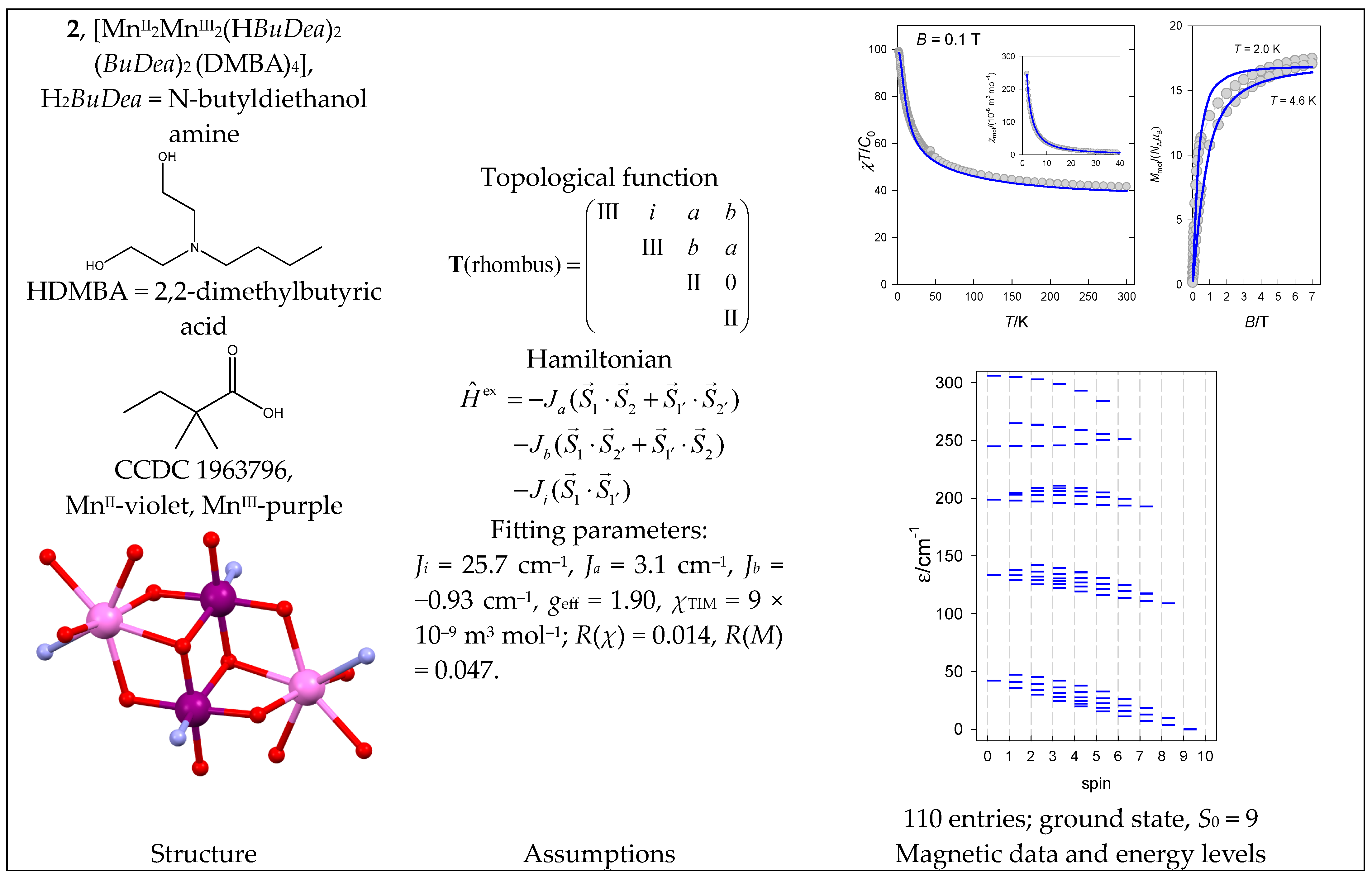
The complex [MnII2MnIII2(HBuDea)2(BuDea)2(DMBA)4] (2) with a {MnII(MnIIIMnIII)MnII} core is somehow analogous to 1, but with a different coupling path: the peripheral MnII centers are coupled to both inner MnIII ones. The crystallographic Mn1 centers related to MnIII are labeled as 1 and 1′, while the Mn2 centers corresponding to MnII are labeled as 2 and 2′ centers. Then, Ji refers to the inner diad J(MnIII-MnIII) with separation, Mn1-Mn1 = 3.17 Å; Ja and Jb correspond to two different pairs, MnII-MnIII, for separations Mn2-Mn1 = 3.24 and 3.41 Å, respectively. The magnetic data are shown in Figure 3.
Two MnIII–O–MnIII superexchange pathways with a bond angle of 98° transmit an exchange coupling of a ferromagnetic nature with positive Ji. The slightly positive Ja reflects two superexchange pathways with MnIII–O–MnII bond angles of 89° and 107°. The slightly negative Jb relates to two superexchange pathways with MnIII–O–MnII bond angles of 103° and 109°. A simplified model that merges Ja = Jb provides geff = 1.95, Ji = 25.0 cm−1, Ja = 0.97 cm−1, χTIM = 9 × 10⁻⁹ m3 mol−1; R(χ) = 0.041, R(M) = 0.054. The spectrum of energy levels for 2 is completely different from 1, as the ferromagnetic interaction between the inner pair of MnIII centers, Ji >> 0, now dominates (Figure 3).
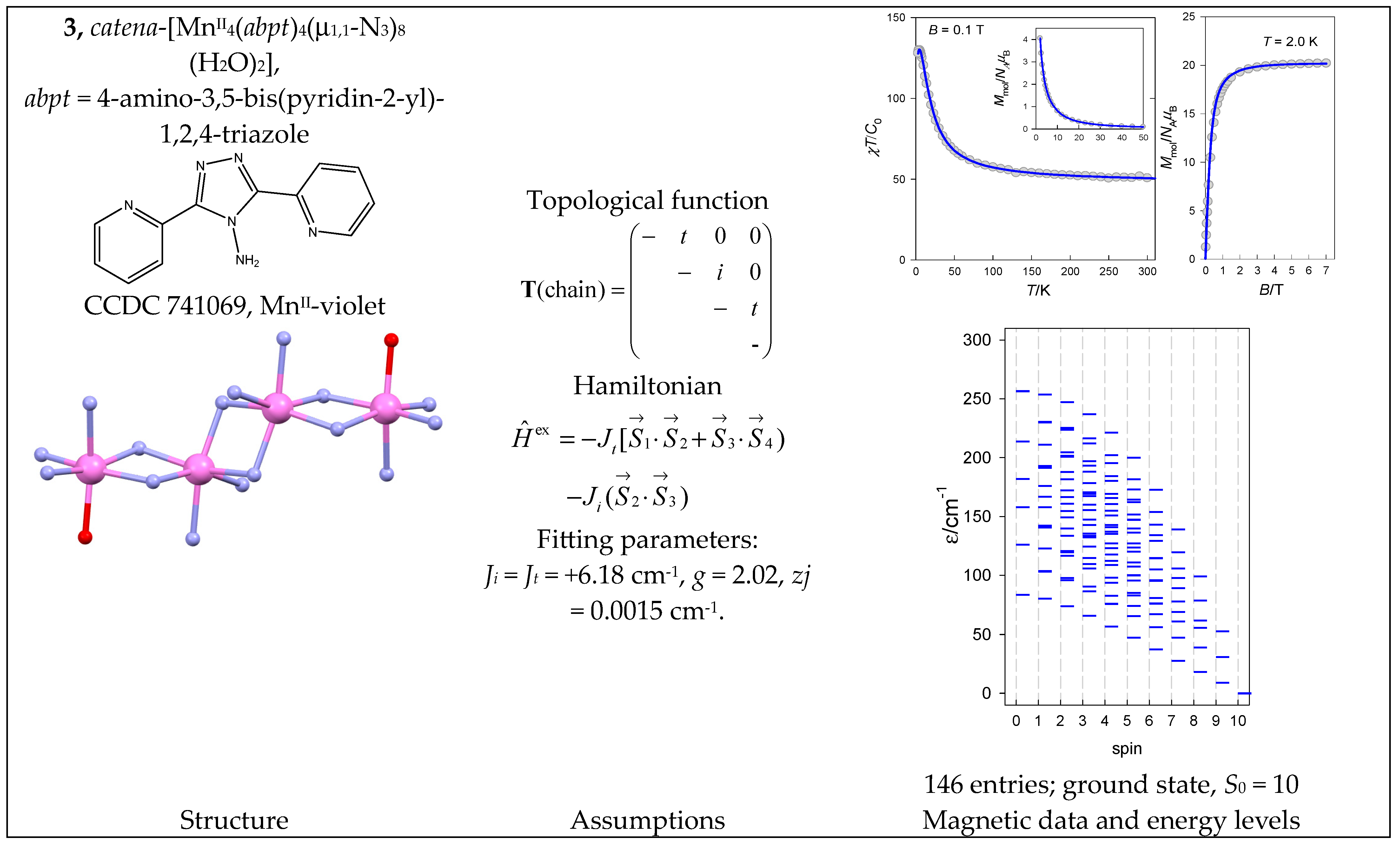
The complex catena-[MnII4(abpt)4(μ1,1-N3)8(H2O)2] (3) is a typical chain of uniform spins whose Hamiltonian contains two different coupling constants Jt (terminal) and Ji (internal). The magnetic functions presented in Figure 4 were fitted assuming the ferromagnetic exchange; the ground state, S0 = Smax = 10, is also confirmed by the saturation of the magnetization.
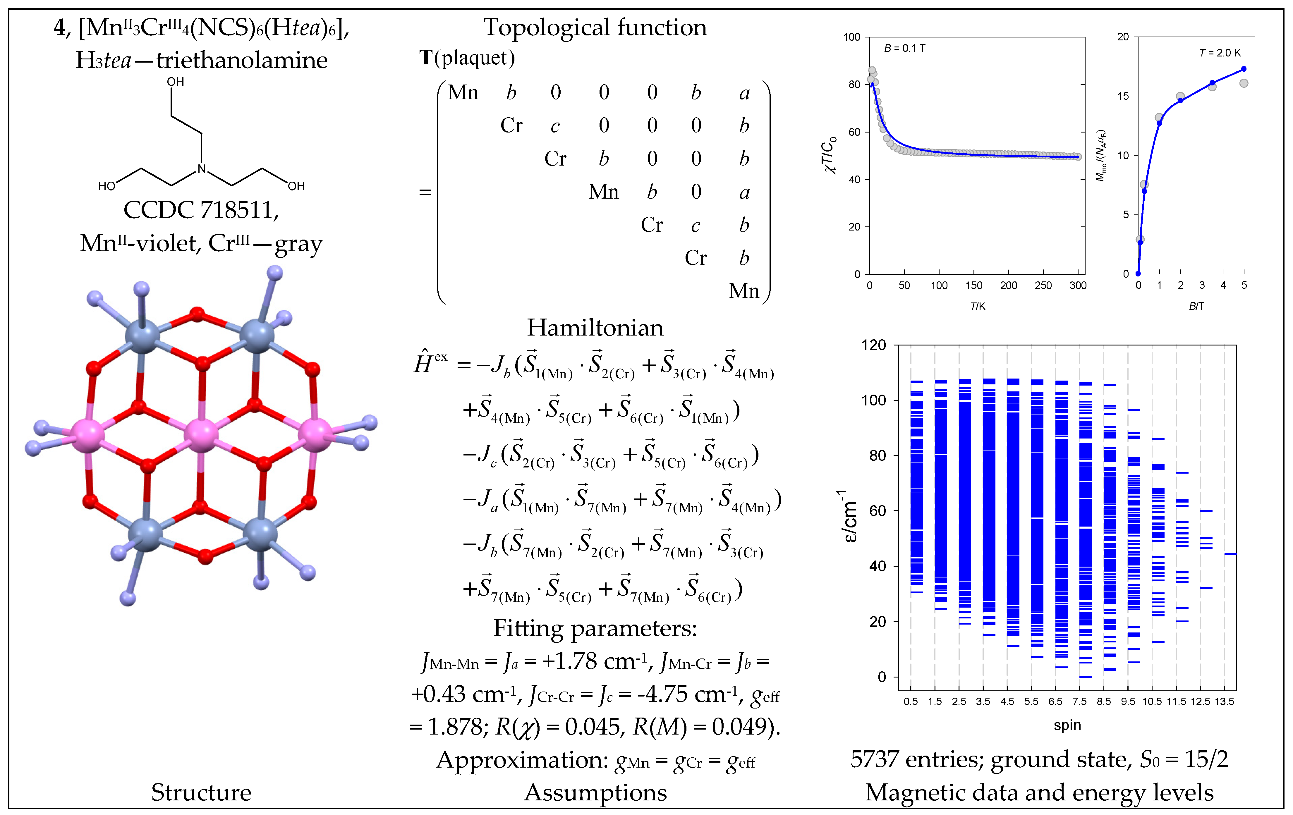
The complex [MnII3CrIII4(NCS)6(Htea)6] (4) with a {MnII3CrIII4} core has the shape of a plaquet, where the trinuclear chain MnIII…MnIII…MnIII is decorated with two pairs of CrIII centers. An appropriate Hamiltonian, together with the topological matrix for the chosen numbering, is shown in Figure 5. The energy spectrum of 4 has an “irregular structure” with a ground state of neither the lowest nor the highest spin.
Magnetic data for catena-[MnII(poxap)MnII(ac)4MnII(poxap)] (5) show that the magnetic susceptibility gradually decreases upon cooling but then rises abruptly (Figure 6). A simultaneous fitting of susceptibility and magnetization for 5 yielded J = −4.56 cm−1, g = 1.96, D = −0.02 cm−1, and zj/hc = +0.054 cm−1. This is also the case for the irregular energy spectrum.
The octanuclear complex [MnIII8(μ3-O)4(μ-pz)8(μ-OMe)4(OMe)4] (6) with a {MnIII8} core has a complex architecture. The coupling path involves three exchange constants (Figure 7).
6.2. Fe(III) Complexes
The heterometallic complex tetrahedro@tetrahedro-[FeIII4(μ4-O)4MnIII4(L)8(DMF)4] ·2DMF (7) contains an {FeIII4MnIII4} core. Its architecture is represented by the central FeIII4 unit arranged in a tetrahedron, which is further decorated by four peripheral MnIII centers (a tetrahedron within a tetrahedron); this is somewhat similar to 5. There might be two distinct coupling pathways Ja(FeIII-FeIII) and Jb(FeIII-MnIII) of an antiferromagnetic nature (Figure 8). The averaged bond angles are Fe-O-Fe = 103° and Mn-O-Fe = 113°.
The polynuclear complex catena-[CoIII6FeIII6(HL)2(L)10(μ-Cl)2]·8DMF (8) contains a magnetoactive {FeIII6} chain decorated with six diamagnetic CoIII centers. This means there are two coupling constants: Jt (terminal) and Ji (internal). The profile of the product function suggests antiferromagnetic exchange (Figure 9).
The [FeII(CN)6{FeIII(salpet)}6]Cl2 complex (9) contains a central unit {FeII(CN)6} with six {FeIII(salpet)}+ moieties attached. The FeII center in a strong crystal field is non-magnetic. Six SA = 5/2 centers provide the resulting spins, S = 0 through 15. However, 9 shows a thermally induced spin crossover, as shown in Figure 10, probably from three low-spin plus three high-spin states. The susceptibility upon cooling only increases and does not show the maximum typical of the S0 = 0 ground state. However, this could be masked by paramagnetic impurity because of S = 5/2 mononuclear fragments.
There are three similar complexes with slightly modified ligands, L = La, Lb, and Lc, of which [FeII(CN)6{FeIII(Lb)}6]Cl2·H2O (10b) is analyzed below. The core {FeIII6FeII} of the complex is identical to 9, but the complex is high-spin over the entire temperature range (Figure 11). The first model considers fifteen J constants; the second considers twelve Jc(cis)-constants and omits three J(trans).
The third model includes a single-center axial zero-field splitting parameter, D. Because of D, the Hamiltonian yields matrix elements that are off-diagonal in the spin quantum number, and the S-blocking of the total interaction matrix is not valid. To make the calculation feasible, a symmetry-adapted local basis set was generated using the spin permutation symmetry of the spin Hamiltonian and the D6 point group of symmetry. Consequently, the entire interaction matrix is divided according to irreducible representations into blocks A1 (K = 4291), A2 (K = 3535), B1 (K = 4145), B2 (K = 3605), E1 (K = 15,470), and E2 (K = 15,610).
The complex [FeIII7O3(O2CPh)9(mda)3(H2O)] (11) was prepared and investigated in depth elsewhere [44]. Its architecture suggests a combination of a ring and a star with magnetic data indicating antiferromagnetic coupling. Magnetostructural correlations (MSCs) predict that there are four coupling constants in play, Ja = −45.0, Jb = −12.6, Jc = −6.2, and Jd = −30.0 cm−1 (for notation −2J between spins), yielding the ground state S0 = 5/2. To confirm this prediction, a spin-Hamiltonian with empirical (MSC) coupling constants (rescaled to −J notation) was worked out, and the predicted magnetic functions are plotted in Figure 12. The course of the product function matches the experimental findings [44]. The resulting energy levels confirm the ground state, S0 = 5/2 (not 1/2), separated from the lowest excited state, S = 7/2, by ΔE = 157 cm−1
The complex [FeIII8(µ4-O)4(µ-pz)12Cl4] (12) has a tetrahedro@tetrahedro-{FeIII8} core. Susceptibility data are shown in Figure 13 and indicate massive antiferromagnetic coupling. The topological function suitable for the data fitting contains two coupling constants, Ji (inner tetrahedron, 6×) and Jo (outer 12×). There is an obstacle—the large size of the largest block n(S = 5) = 16576. The problem of diagonalization of such matrices was avoided by using the symmetry point group, D2.
The fitting procedure provided the coupling constants Ji = −2.1, Jo = −50.6 cm−1, and g = 2.0 (fixed); the energy spectrum is drawn in Figure 13. Only a very limited part of the energy spectrum is thermally populated; this explains the temperature evolution of the product function. The small value of Ji refers to six coupling pathways inside the inner tetrahedron with an average angle of 12 bonds: Fe-O-Fe = 96.7°. The bond angles of Fei-O-Feo average 119.7°, rationalizing the much more negative Jo.
The complex cyclo-[FeIII10(bdtbpza)10(MeO)20] (13) is a typical ring system (wheel) that has only one J-constant between neighboring members. Its magnetic functions are presented in Figure 14, indicating an exchange coupling of an antiferromagnetic nature. Fitting 10-membered FeIII systems is an unrealistic task because there are M = 4,395,456 zero-field states, and the biggest S-block has a dimension of n(S = 5) = 484,155. Therefore, we restricted ourselves to the cyclo-{FeIII8} model with M = 135,954 and n(S = 5) = 16,576, hoping it would work satisfactorily. The construction of the topological matrix and the spin-Hamiltonian are straightforward; the fitting procedure yielded J = −8.58 cm−1, g = 2.0; xPI = 0.0049. For a more simplified cyclo-{FeIII6} model with M = 4332 and n(S = 4) = 609, the calculated parameters were J = −8.64 cm−1, xPI = 0.0064. The energy levels for a such model are displayed in Figure 14.
6.3. Co(II) Complexes
The complex cyclo-[CoII6CoIII(thmp)2(acac)6(ada)3] (14) with a {CoII6CoIII} core is a ring system indicating only a single exchange coupling constant. However, there is some asymmetry in the Co…Co separations (3.034, 3.145, 3.032, 3.169, 3.174, 3.038 Å), and therefore, two different J-constants were considered (Figure 15).
It is well known that single-ion magnetic anisotropy plays an important role in hexacoordinate Co(II) complexes. This is expressed by the axial zero-field splitting parameter, D, and was involved in the spin Hamiltonian for 14 (see Equation (11)). The magnetic data are shown in Figure 15, and the fitting procedure yielded Ja = 0.95, Jb = 5.11 cm−1, g = 2.65, and D = 79 cm−1. The modeled energy levels for D = 0 are plotted in Figure 15. (The D-value makes the spin no longer a good quantum number, and the classification of zero-field states using spin becomes meaningless).
The complex bis-cyclo-[CoII11CoIII2(thmp)4(Me3CCOO)4(acac)6(OH)4(H2O)4] (Me3CCOO)2·H2O (15) with a {CoII11CoIII2} core is the result of the fusion of two ring systems. The magnetic functions are shown in Figure 16. Treating the eleven S = 3/2 centers is a serious problem because there are now K = 4,194,304 energy levels in play. The task was simplified by considering a ring of only seven cyclo-[A7] centers with K = 16,384 levels in the basis of uncoupled functions. The use of permutation symmetry made it possible to divide the entire matrix into subblocks. A new set of symmetry-adapted spin basis sets was created using the D7 point group. The total interaction matrix is split into submatrices A1 (N = 1300), A2 (N = 1044), E1 (N = 4680), E2 (N = 4680), and E3 (N = 4680). Then, a fitting procedure based on both temperature and field-dependent magnetic data resulted in J = 3.34 cm−1, D = 63.8 cm−1, and g = 2.64. The increased value of the g-factor relative to the free-electron, ge = 2.0, reflects the presence of the orbital angular momentum; it is manifested by a magnetization per formula unit that exceeds the value of M1 ~ 21 μB. The energy levels in the approximation of the [Co7] ring are drawn in Figure 16.
The complex [CoII9CoIII3(μ3-O)3-(μ1,1,1-N3)(μ1,1-N3)3(μ3-L)9(μ-L)6](ClO4)2·H3tea·9.5H2O (16) contains a {CoII9CoIII3} core and it has the architecture of a plaquet. The magnetic data are plotted in Figure 17, which shows the hook at the lowest temperature of the product function. Three inner CoII centers forming a triangle are coupled by double bridges with angles i{90.6(N), 103.5(O)}, and the inner-outer paths include double bridges of o{100.2, 101.2} and o{94.1, 104.5}. S-blocking offered the highest matrix to be diagonalized at a size of n(S = 7/2) = 5300, and the fitting procedure yielded Ji = −10.3 cm−1, Jo = +0.98 cm−1, and g = 2.58. The zero-field splitting was omitted, which prevents a reliable reconstruction of the low-temperature data.
6.4. Ln(III) Complexes
Apart from Gd(III), lanthanide complexes are typically known as highly anisotropic systems, exhibiting large g-factor differences (gz—gxy). Because of the addition of spin and angular momenta, the total angular momentum, J = L + S, is in play, giving rise to spin–orbit multiplets. The crystal field is a minor effect because the f-orbitals are effectively screened against point charges generated by the ligands. Stevens operators, , however, imitate the effect of a crystal field, where the contributions cover several members (k—tensor rank, q—component). These operators cause J-multiplets to be split and mixed into zero-field-slitting levels. The omission of these factors has an important effect on the reconstruction of the magnetization at low temperatures: the calculated magnetization is much higher than the experimental data.
The complex triangulo-[ErIII3Cl(L)3(OH)2(H2O)5]Cl3 (17) has an {ErIII3} core referring to an isosceles triangle (there is one additional Er-Cl bond). The Er-Er distances are 3.505, 3.509, and 3.478 Å, indicating two coupling constants. The bond angles along the path a{97, 99} and along b{95, 98} deg predict that Ja and Jb will be small. The product function gradually decreases upon cooling, reflecting the prevailing antiferromagnetic exchange (Figure 18). The susceptibility data were fitted using a Hamiltonian that includes the total angular momentum, J = S + L, instead of the net spin, where each Er(III) center offers JA = 15/2 (the free-atom multiplet is 4I15/2 with gJ = 6/5). The molecular J-value varies between 1/2 and 45/2, yielding an irregular energy spectrum; the ground state is J0 = 21/2 (Figure 18). When only the ground state is populated at a sufficiently low temperature, the estimated magnetization will be M0 ~ gJ0 ~ 12.3 μB.
The tetranuclear complex [DyIII4(L)4(μ2-OH)2Cl4]Cl2·EtOH (18) with a {DyIII4} core is topologically analogous to 2 (rhombus). It has three coupling paths with Ja{107, 112} and Ji{109} for an inner diad and Jc{100, 99, 80-Cl}, where data in parentheses refer to bond angles. Upon cooling, the product function remains almost constant and then decreases (Figure 19). The energy spectrum ranges from Jmin = 0 to Jmax = 4·(15/2) = 60/2; the ground state is J0 = 0 (Figure 19). The leading coupling is an inner diad, Ji < 0, and is responsible for the overall antiferromagnetic exchange. This is the main difference compared with the 2a with an analogous topology.
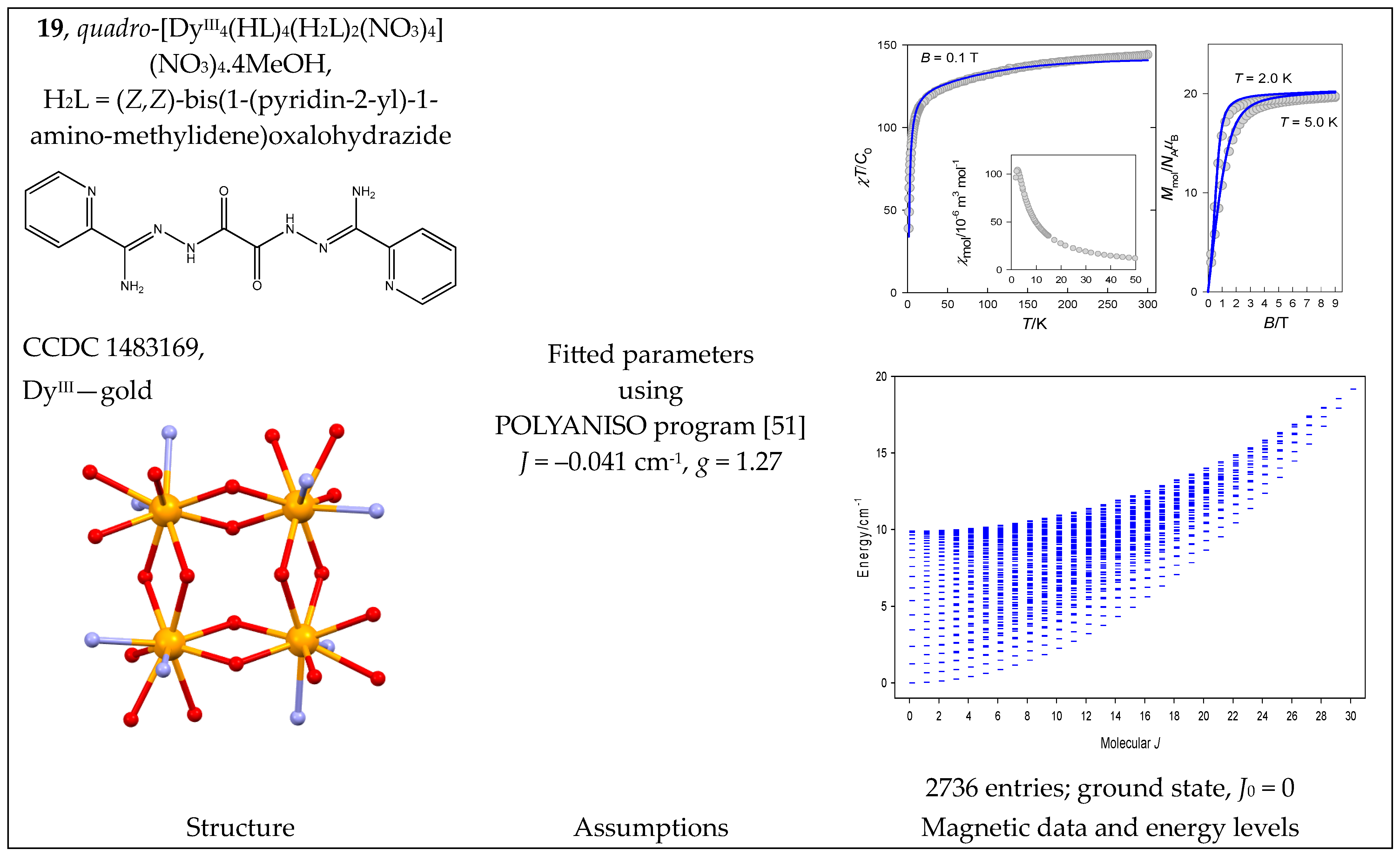
The complex quadro-[DyIII4(HL)4(H2L)2(NO3)4](NO3)4·4MeOH (19) can be considered a four-membered ring with a single J-constant. The Dy-O-Dy bond angles are 110—115°, so a negative J is expected. The magnetic data are shown in Figure 20; they were reconstructed with J = −0.03 cm−1 [51]. The fitting procedure yielded J = −0.041 cm−1, g = 1.27.
The heteronuclear complex [(H2O)6DyIII2(μ2-L)2(μ3-O)4CuII5(μ2-Cl)2] (20) with a plaquet architecture contains two DyIII centers that are non-coordinated: two tetracoordinate CuII, two pentacoordinate CuII, and one hexacoordinate CuII center. The magnetic functions are shown in Figure 21 with an unusual course of product function: it gradually decreases during cooling but then rises sharply. The width of the energy spectrum is J = 1/2 to 35/2, and the ground state is J0 = 25/2. The irregular shape of the energy spectrum causes the product function to increase upon cooling since the magnetically productive ground state is then increasingly more populated; this is regardless of antiferromagnetic exchange (Ja and Jb < 0) when one would (erroneously) expect J0 = 1/2.
7. Conclusions
This theoretical work outlines a general method of handling exchange coupling in polynuclear spin systems. The method avoids the case-by-case coupling of the Kambe method, which works in many cases but also fails in many cases. The method uses a whole apparatus of irreducible tensor operators. The exchange Hamiltonian can include or skip any combination of pairwise interactions between the constituting spins (or alternatively, the total angular momenta, J). Spins at the centers can be of any size (for example, S = 5/2 or J = 15/2), non-uniform, and set in any order. The matrix elements of the spin-Hamiltonian are taken into a reduced form (free of projections of angular momenta) and then decoupled into the elementary reduced matrix elements using 9j-symbols (numbers that couple four angular momenta). The full set of intermediate quantum numbers is contained in the coupling history matrix (CHM); the matrices of the operator ranks (ORs) and the intermediate operator ranks (IORs) are evaluated in an automated way with no assistance from the user. The rate-limiting step is the diagonalization of the (symmetric) blocks of the Hamiltonian matrix, although only the eigenvalues are required. For example, for an {FeIII8} system with spins with SA = 5/2, the largest block for S = 5 has a dimension of 16,576.
The user’s task is to set
- A number of magnetic centers, N, and spins, SA, on individual centers in any order and size;
- The topological matrix T(A,B), which defines the coupling path; this contains a trial set of exchange-coupling constants, J(A,B), that will be optimized; their number is less or equal to N(N—1)/2;
- The value of the g-factor, which must be uniform (geff), to correctly exploit the blocking of the Hamiltonian matrix according to molecular spin.
The zero-field energy levels, magnetic susceptibility (temperature dependence). and magnetization (field dependence) are obtained as outputs and processed by an optimization procedure to obtain the minimum error function, F(Mo, Mc; χo, χc), composed of observed (o) and calculated (c) magnetic functions. Susceptibility and magnetization data are optimized simultaneously. This is a very strict requirement: sometimes excellent fits are obtained only for the susceptibility and magnetization data.
In practical applications, the method is limited only by the memory and speed of the user’s computer. The inclusion of the non-uniform g-factors (gA), zero-field splitting (DA, EA), asymmetric exchange (DAB, EAB), and antisymmetric exchange (aAB) cause the key advantage of the blocking to collapse.
During the modeling of spin chains/rings/convex polyhedrons, several important findings were revealed.
One would expect that, for antiferromagnetic coupling, the ground states should either be S0 = 0 or ½. This is not true in general, as there are systems that have an irregular energy spectrum where the ground state falls between Smin and Smax. This is always the case for star-like architectures and odd catena-[AN] chains for N = 3, 5, 7, 9, … S = 3/2, and 5/2.
For the antiferromagnetically coupled cyclo-[AN] system, the ground state is four-fold degenerate (two Kramers doublets with S = 1/2) if Ns is a half-integer. If Ns is an integer, the ground state is non-degenerate (S = 0).
For cyclo-[A9, s = 1/2], the ground state is doubly degenerate S0 = 1/2 (twice). The ground state of catena-[A9, s = 1/2] is S0 = 1/2 (×1), and the first excited state, S1 = 1/2 (×1), lies at an energy of −0.75J.
Applications to real systems confirm that the method is applicable to homonuclear systems with uniform g-factors and systems with similar g-factors. For polynuclear lanthanides, the susceptibility can be recovered satisfactorily; however, the magnetization is overestimated since the asymmetry terms provided by the Stevens operators are missing.
Author Contributions
All authors contributed equally to all sections. All authors have read and agreed to the published version of the manuscript.
Funding
Slovak grant agencies (APVV 19-0087, VEGA 1/0086/21, and VEGA 1/0191/22) are acknowledged for their financial support.
Institutional Review Board Statement
Not applicable.
Informed Consent Statement
Not applicable.
Data Availability Statement
The magnetic data are available from the corresponding author upon request.
Acknowledgments
The authors are thankful to Radovan Herchel (PU University, Olomouc, Czech Republic) for his valuable comments and agreement to share some raw magnetic data.
Conflicts of Interest
The authors declare no conflict of interest.
References
- Kambe, K. On the Paramagnetic Susceptibilities of Some Polynuclear Complex Salts. J. Phys. Soc. Jpn. 1950, 5, 48–51. [Google Scholar] [CrossRef]
- Kahn, O. Molecular Magnetism; VCH: Weinheim, Germany, 1993; ISBN 9780471188384. [Google Scholar]
- Rose, M.E. Elementary Theory of Angular Momentum; Wiley: New York, NY, USA, 1957; ISBN 9780471735243. [Google Scholar]
- Fano, U.; Racah, G. Irreducible Tensorial Sets; Academic Press: New York, NY, USA, 1959; ISBN 9781483230597. [Google Scholar]
- Griffith, J.S. The Irreducible Tensor Method for Molecular Symmetry Group; Courier Dover Publications: Mineola, NY, USA; Prentice-Hall: London, UK, 1962. [Google Scholar]
- Brink, D.M.; Satchler, G.R. Angular Momentum; Claredon Press: Oxford, UK, 1962. [Google Scholar]
- Judd, B.R. Operator Techniques in Atomic Spectroscopy; McGraw–Hill: New York, NY, USA, 1963; ISBN 9781114630574. [Google Scholar]
- Wybourne, B.G. Spectroscopic Properties of Rare Earths; Wiley: New York, NY, USA, 1965; ISBN 9780470965078. [Google Scholar]
- Jucys, A.P.; Savukynas, A.V. Mathematical Foundations of the Atomic Theory; Mintis: Viljnus, Lithuania, 1972. (In Russian) [Google Scholar]
- Varshalovich, D.A.; Moskalev, A.N.; Chersonskii, V.K. Quantum Theory of Angular Momentum; Nauka: Saint Petersburg, Russia, 1975. (In Russian) [Google Scholar]
- Silver, B.L. Irreducible Tensor Method; Academic Press: New York, NY, USA, 1976. [Google Scholar]
- Sobelman, I.I. Atomic Spectra and Radiative Transitions; Springer: Berlin/Heidelberg, Germany, 1979; ISBN 9783662059050. [Google Scholar] [CrossRef]
- Zare, R.N. Angular Momentum: Understanding Spatial Aspects in Chemistry and Physics; Wiley: New York, NY, USA, 1988; ISBN 9780471858928. [Google Scholar]
- Tsukerblat, B.S. Group Theory in Chemistry and Spectroscopy; Academic Press: London, UK, 1994; ISBN 9780127022857. [Google Scholar]
- Lueken, H. Magnetochemie; Teubner: Stuttgart, Germany, 1999; ISBN 9783519035305. (In German) [Google Scholar]
- Bencini, A.; Gatteschi, D. Electron Paramagnetic Resonance of Exchange Coupled Systems; Springer: Berlin/Heidelberg, Germany, 1990; ISBN 9783642746017. [Google Scholar]
- Borras-Almenar, J.; Clemente-Juan, J.; Coronado, E.; Palii, A.; Tsukerblat, B. Magnetic Exchange between Orbitally Degenerate Ions: A New Development for the Effective Hamiltonian. J. Phys. Chem. A 1998, 102, 200–213. [Google Scholar] [CrossRef]
- Ceulemans, A.; Chibotaru, L.; Heylen, G.; Pierloot, K.; Vanquickenborne, L. Theoretical Models of Exchange Interactions in Dimeric Transition-Metal Complexes. Chem. Rev. 2000, 100, 787–806. [Google Scholar] [CrossRef] [PubMed]
- Palii, A.; Tsukerblat, B.; Coronado, E.; Clemente-Juan, J.; Borras-Almenar, J. Orbitally dependent magnetic coupling between cobalt(II) ions: The problem of the magnetic anisotropy. J. Chem. Phys. 2003, 118, 5566–5581. [Google Scholar] [CrossRef]
- Mironov, V.; Chibotaru, L.; Ceulemans, A. Mechanism of a Strongly Anisotropic MoIII–CN–MnII Spin–Spin Coupling in Molecular Magnets Based on the [Mo(CN)7]4- Heptacyanometalate: A New Strategy for Single-Molecule Magnets with High Blocking Temperatures. J. Am. Chem. Soc. 2003, 125, 9750–9760. [Google Scholar] [CrossRef] [PubMed]
- Palii, A.; Tsukerblat, B.; Clemente-Juan, J.M.; Coronado, E. Magnetic exchange between metal ions with unquenched orbital angular momenta: Basic concepts and relevance to molecular magnetism. Int. Rev. Phys. Chem. 2010, 29, 135–230. [Google Scholar] [CrossRef]
- Schnale, R.; Schnack, J. Calculating the energy spectra of magnetic molecules: Application of real- and spin-space symmetries. Int. Rev. Phys. Chem. 2010, 29, 403–452. [Google Scholar] [CrossRef]
- Borras-Almenar, J.J.; Clemente-Juan, J.M.; Coronado, E.; Tsukerblat, B.S. High-Nuclearity Magnetic Clusters: Generalized Spin Hamiltonian and Its Use for the Calculation of the Energy Levels, Bulk Magnetic Properties, and Inelastic Neutron Scattering Spectra. Inorg. Chem. 1999, 38, 6081–6088. [Google Scholar] [CrossRef]
- Tsukerblat, B. Group-theoretical approaches in molecular magnetism: Metal clusters. Inorg. Chim. Acta 2008, 361, 3746–3760. [Google Scholar] [CrossRef]
- Boyarchenkov, A.S.; Bostrem, I.G.; Ovchinnikov, A.S. Quantum magnetization plateau and sign change of the magnetocaloric effect in a ferrimagnetic spin chain. Phys. Rev. B 2007, 76, 224410. [Google Scholar] [CrossRef]
- Borras-Almenar, J.J.; Clemente-Juan, J.M.; Coronado, E.; Tsukerblat, B.S. MAGPACK1 A package to calculate the energy levels, bulk magnetic properties, and inelastic neutron scattering spectra of high nuclearity spin clusters. J. Comp. Chem. 2001, 22, 985–991. [Google Scholar] [CrossRef]
- Schnack, J.; Luban, M. Rotational modes in molecular magnets with antiferromagnetic Heisenberg exchange. Phys. Rev. B 2000, 63, 014418. [Google Scholar] [CrossRef]
- Waldmann, O. Spin dynamics of finite antiferromagnetic Heisenberg spin rings. Phys. Rev. B 2001, 65, 024424. [Google Scholar] [CrossRef]
- Waldmann, O. E-band excitations in the magnetic Keplerate molecule Fe30. Phys. Rev. B 2007, 75, 012415. [Google Scholar] [CrossRef]
- Waldmann, O.; Stamatatos, T.C.; Christou, G.; Güdel, H.U.; Sheikin, I.; Mutka, H. Quantum Phase Interference and Néel-Vector Tunneling in Antiferromagnetic Molecular Wheels. Phys. Rev. Lett. 2009, 102, 157202. [Google Scholar] [CrossRef]
- Boča, R. Zero-field splitting in metal complexes. Coord. Chem. Rev. 2004, 248, 757–815. [Google Scholar] [CrossRef]
- Boča, R.; Herchel, R. Antisymmetric exchange in polynuclear metal complexes. Coord. Chem. Rev. 2010, 254, 2973–3025. [Google Scholar] [CrossRef]
- Bärwinkel, K.; Schmidt, H.-J.; Schnack, J. Structure and relevant dimension of the Heisenberg model and applications to spin rings. J. Magn. Magn. Mater. 2000, 212, 240–250. [Google Scholar] [CrossRef]
- Uhrecký, R.; Moncoľ, J.; Koman, M.; Titiš, J.; Boča, R. Structure and magnetism of a Mn(III)–Mn(II)–Mn(II)–Mn(III) chain complex. Dalton Trans. 2013, 42, 9490–9494. [Google Scholar] [CrossRef] [PubMed]
- Reis Conceição, N.; Nesterova, O.V.; Rajnák, C.; Boča, R.; Pombeiro, A.J.L.; Guedes da Silva, M.F.C.; Nesterov, D.S. New members of the polynuclear manganese family: MnII2MnIII2 single-molecule magnets and Mn II3Mn III8 antiferromagnetic complexes. Synthesis and magnetostructural correlations. Dalton Trans. 2020, 49, 13970–13985. [Google Scholar] [CrossRef]
- Meng, Z.-S.; Yun, L.; Zhang, W.-X.; Hong, C.-G.; Herchel, R.; Ou, Y.-C.; Leng, J.-D.; Peng, M.-X.; Lin, Z.-J.; Tong, M.-L. Reactivity of 4-amino-3,5-bis(pyridin-2-yl)-1,2,4-triazole, structures and magnetic properties of polynuclear and polymeric Mn(II), Cu(II) and Cd(II) complexes. Dalton Trans. 2009, 10284–10295. [Google Scholar] [CrossRef] [PubMed]
- Semenaka, V.V.; Nesterova, O.V.; Kokozay, V.N.; Zybatyuk, R.I.; Shishkin, O.V.; Boča, R.; Shevchenkod, D.V.; Huang, P.; Styring, S. Direct synthesis of an heterometallic {MnII3CrIII4} wheel by decomposition of Reineckes salt. Dalton Trans. 2010, 39, 2344–2349. [Google Scholar] [CrossRef] [PubMed]
- Herchel, R.; Boča, R.; Gembický, M.; Falk, K.; Fuess, H.; Haase, W.; Svoboda, I. Magnetic Properties of a Manganese(II) Trinuclear Complex Involving a Tridentate Schiff-Base Ligand. Inorg. Chem. 2007, 46, 1544–1546. [Google Scholar] [CrossRef] [PubMed]
- Babic-Samardzija, K.; Baran, P.; Boča, R.; Herchel, R.; Raptis, R.G.; Velez, C.L. Structural and magnetic susceptibility study of an octanuclear MnIII-oxo-pyrazolido complex. Polyhedron 2018, 149, 142–147. [Google Scholar] [CrossRef]
- Nesterova, O.V.; Chygorin, E.N.; Kokozay, V.N.; Omelchenko, I.V.; Shishkin, O.V.; Boča, R.; Pombeiro, A.J.L. A self-assembled octanuclear complex bearing the uncommon close-packed {Fe4Mn4(μ4-O)4(μ-O)4} molecular core. Dalton Trans. 2015, 44, 14918–14924. [Google Scholar] [CrossRef]
- Chygorin, E.N.; Kokozay, V.N.; Omelchenko, I.V.; Shishkin, O.V.; Titiš, J.; Boča, R.; Nesterov, D.S. Direct synthesis of a {Co III6Fe III6} dodecanuclear complex, revealing an unprecedented molecular structure type. Dalton Trans. 2015, 44, 10918–10922. [Google Scholar] [CrossRef]
- Boča, R.; Šalitroš, I.; Kožíšek, J.; Linares, J.; Moncoľ, J.; Renz, F. Spin crossover in a heptanuclear mixed-valence iron complex. Dalton Trans. 2010, 39, 2198–2200. [Google Scholar] [CrossRef]
- Šalitroš, I.; Boča, R.; Herchel, R.; Moncoľ, J.; Nemec, I.; Ruben, M.; Renz, F. Mixed-Valence Heptanuclear Iron Complexes with Ferromagnetic Interaction. Inorg. Chem. 2012, 51, 12755–12767. [Google Scholar] [CrossRef]
- Hale, A.R.; Lott, M.E.; Peralta, J.E.; Foguet-Albiol, D.; Abboud, K.A.; Christou, G. Magnetic Properties of High-Nuclearity Fex-oxo (x = 7, 22, 24) Clusters Analyzed by a Multipronged Experimental, Computational, and Magnetostructural Correlation Approach. Inorg. Chem. 2022, 61, 11261–11276. [Google Scholar] [CrossRef]
- Baran, P.; Boča, R.; Chakraborty, I.; Giapintzakis, J.; Herchel, R.; Huang, Q.; McGrady, J.E.; Raptis, R.G.; Sanakis, Y.; Simopoulos, A. Synthesis, Characterization, and Study of Octanuclear Iron-Oxo Clusters Containing a Redox-Active Fe4O4-Cubane Core. Inorg. Chem. 2008, 47, 645–655. [Google Scholar] [CrossRef]
- Gajewska, M.J.; Bieńko, A.; Herchel, R.; Haukka, M.; Jerzykiewicz, M.; Ożarowski, A.; Drabent, K.; Hung, C.-H. Iron(III) bis(pyrazol-1-yl)acetate based decanuclear metallacycles: Synthesis, structure, magnetic properties and DFT calculations. Dalton Trans. 2016, 45, 15089–15096. [Google Scholar] [CrossRef]
- Leng, J.-D.; Xing, S.-K.; Herchel, R.; Liu, J.-L.; Tong, M.-L. Disklike Hepta- and Tridecanuclear Cobalt Clusters. Synthesis, Structures, Magnetic Properties, and DFT Calculations. Inorg. Chem. 2014, 53, 5458–5466. [Google Scholar] [CrossRef] [PubMed]
- Zheng, L.-L.; Leng, J.-D.; Herchel, R.; Lan, Y.-H.; Powell, A.K.; Tong, M.-L. Anion-Dependent Facile Route to Magnetic Dinuclear and Dodecanuclear Cobalt Clusters. Eur. J. Inorg. Chem. 2010, 2010, 2229–2234. [Google Scholar] [CrossRef]
- Gebrezgiabher, M.; Schlittenhardt, S.; Rajnák, C.; Kuchár, J.; Sergawie, A.; Černák, J.; Ruben, M.; Thomas, M.; Boča, R. Triangulo-{ErIII3} complex showing field supported slow magnetic relaxation. RSC Adv. 2022, 12, 21674–21680. [Google Scholar] [CrossRef] [PubMed]
- Gebrezgiabher, M.; Schlittenhardt, S.; Rajnák, C.; Sergawie, A.; Ruben, M.; Thomas, M.; Boča, R. A Tetranuclear Dysprosium Schiff Base Complex Showing Slow Relaxation of Magnetization. Inorganics 2022, 10, 66. [Google Scholar] [CrossRef]
- Gusev, A.; Herchel, R.; Nemec, I.; Shuľgin, V.; Eremenko, I.L.; Lyssenko, K.; Linert, W.; Trávníček, Z. Tetranuclear Lanthanide Complexes Containing a Hydrazone-type Ligand. Dysprosium [2 × 2] Gridlike Single-Molecule Magnet and Toroic. Inorg. Chem. 2016, 55, 12470–12476. [Google Scholar] [CrossRef]
- Mičová, R.; Rajnák, C.; Titiš, J.; Moncoľ, J.; Nováčiková, J.; Bieńko, A.; Renz, F.; Boča, R. to be published.
- Delfs, C.; Gatteschi, D.; Pardi, L.; Sessoli, R.; Weighardt, K.; Hanke, D. Magnetic properties of an octanuclear iron(III) cation. Inorg. Chem. 1993, 32, 3099–3103. [Google Scholar] [CrossRef]
- Waldmann, O. Symmetry and energy spectrum of high-nuclearity spin clusters. Phys. Rev. 2000, B61, 6138–6144. [Google Scholar] [CrossRef]
- Schnack, J. Exact diagonalization techniques for quantum spin systems. Chall. Adv. Comput. Chem. Phys. 2023, 34, 155–177. [Google Scholar] [CrossRef]
- Boča, R. A Handbook of Magnetochemical Formulae; Elsevier: Amsterdam, The Netherlands, 2012; ISBN 9780124160149. [Google Scholar]
- Kunitsky, S.V.; Palii, A.V.; Tsukerblat, B.S.; Clemente-Juan, J.M.; Coronado, E. MVPROG: A program to calculate energy levels and magnetic properties of high nuclearity mixed valence clusters. Moldav. J. Phys. Sci. 2004, 3, 325–328. [Google Scholar]
- Wang, F.; Wang, B.; Wang, M.; Chen, Z. Irreducible tensor operator method study on molecular magnetism: A practical approach and its use for high-nuclearity magnetic cluster. Chem. Phys. Lett. 2008, 454, 177–183. [Google Scholar] [CrossRef]
- Borrás-Almenar, J.; Cardona-Serra, S.; Clemente-Juan, J.; Coronado, E.; Palii, A.; Tsukerblat, B. MVPACK: A Package to Calculate Energy Levels and Magnetic Properties of High Nuclearity Mixed Valence Clusters. J. Comput. Chem. 2009, 31, 1321–1332. [Google Scholar] [CrossRef] [PubMed]
- Chilton, N.F.; Anderson, R.P.; Turner, L.D.; Soncini, A.; Murray, K.S. PHI: A powerful new program for the analysis of anisotropic monomeric and exchange-coupled polynuclear d- and f-block complexes. J. Comput. Chem. 2013, 34, 1164–1175. [Google Scholar] [CrossRef] [PubMed]
- Boča, R. A General Program for Magnetism of Polynuclear Complexes; University of SS Cyril and Methodius: Trnava, Slovakia, 2023. [Google Scholar]
- Schnack, J.; Wendland, O. Properties of highly frustrated magnetic molecules studied by the finite-temperature Lanczos method. Eur. Phys. J. 2010, B78, 535–541. [Google Scholar] [CrossRef]
- Schnack, J.; Ummethum, J. Advanced quantum methods for the largest magnetic molecules. Polyhedron 2013, 66, 28–33. [Google Scholar] [CrossRef]
Figure 1.
Definition of rotations for the D2 and D4 point groups of symmetry.

Figure 2.
Structure and magnetic functions for 1. Magnetic susceptibility is expressed as a dimensionless product function, χT/C0; magnetization per formula unit in Bohr magnetons. According to [34].
Figure 2.
Structure and magnetic functions for 1. Magnetic susceptibility is expressed as a dimensionless product function, χT/C0; magnetization per formula unit in Bohr magnetons. According to [34].

Figure 3.
Structure and magnetic functions for 2. According to [35].
Figure 3.
Structure and magnetic functions for 2. According to [35].

Figure 4.
Structure and magnetic functions for 3. According to [36].
Figure 4.
Structure and magnetic functions for 3. According to [36].

Figure 5.
Structure and magnetic functions for 4. According to [37].
Figure 5.
Structure and magnetic functions for 4. According to [37].

Figure 6.
Structure and magnetic functions for 5. According to [38].
Figure 6.
Structure and magnetic functions for 5. According to [38].

Figure 7.
Structure and magnetic functions for 6. According to [39].
Figure 7.
Structure and magnetic functions for 6. According to [39].

Figure 8.
Structure and magnetic functions for 7. According to [40].
Figure 8.
Structure and magnetic functions for 7. According to [40].

Figure 9.
Structure and magnetic functions for 8. Compare item catena-[A6], s = 5/2, Jn(5×) in Table 10. According to [41].

Figure 10.
Structure and magnetic functions for 9. According to [42].
Figure 10.
Structure and magnetic functions for 9. According to [42].

Figure 11.
Structure and magnetic functions for 10. According to [43].
Figure 11.
Structure and magnetic functions for 10. According to [43].

Figure 12.
Structure and magnetic functions for 11. According to [44].
Figure 12.
Structure and magnetic functions for 11. According to [44].

Figure 13.
Structure and magnetic functions for 12. According to [45].
Figure 13.
Structure and magnetic functions for 12. According to [45].

Figure 14.
Structure and magnetic functions for 13. According to [46].
Figure 14.
Structure and magnetic functions for 13. According to [46].

Figure 15.
Structure and magnetic functions for 14. According to [47].
Figure 15.
Structure and magnetic functions for 14. According to [47].

Figure 16.
Structure and magnetic functions for 15. According to [47].
Figure 16.
Structure and magnetic functions for 15. According to [47].

Figure 17.
Structure and magnetic functions for 16. According to [48].
Figure 17.
Structure and magnetic functions for 16. According to [48].

Figure 18.
Structure and magnetic functions for 17. According to [49].
Figure 18.
Structure and magnetic functions for 17. According to [49].

Figure 19.
Structure and magnetic functions for 18. According to [50].
Figure 19.
Structure and magnetic functions for 18. According to [50].

Figure 20.
Structure and magnetic functions for 19. According to [51].
Figure 20.
Structure and magnetic functions for 19. According to [51].

Figure 21.
Structure and magnetic functions for 20. According to [52].
Figure 21.
Structure and magnetic functions for 20. According to [52].

Table 1.
Dimensions of the S-blocks for N-homospin systems a.
| AN System | Magnetic States, K | Zero-Field States, M | Dimension n(S) from the Lowest Spin, Smin = 0 or 1/2, to the Highest Spin, Smax = N·SA |
|---|---|---|---|
| SA = ½ | |||
| A3 | 8 | 3 | 2, 1 |
| A4 | 16 | 6 | 2, 3, 1 |
| A5 | 32 | 10 | 5, 4, 1 |
| A6 | 64 | 20 | 5, 9, 5, 1 |
| A7 | 128 | 35 | 14, 14, 6, 1 |
| A8 | 256 | 70 | 14, 28, 20, 7, 1 |
| A9 | 512 | 126 | 42, 48, 27, 8, 1 |
| A10 | 1024 | 252 | 42, 90, 75, 35, 9, 1 |
| A11 | 2048 | 462 | 132, 165, 110, 44, 10, 1 |
| A12 | 4096 | 924 | 132, 297, 275, 154, 54, 11,1 |
| A13 | 8192 | 1716 | 429, 572, 429, 208, 65, 12, 1 |
| A14 | 16,384 | 3432 | 429, 1001, 1001, 637, 273, 77, 13, 1 |
| A15 | 32,768 | 6435 | 1430, 2002, 1638, 910, 350, 90, 14 1 |
| SA = 1 | |||
| A3 | 27 | 7 | 1, 3, 2, 1 |
| A4 | 81 | 19 | 3, 6, 6, 3, 1 |
| A5 | 243 | 51 | 6, 15, 15, 10, 4, 1 |
| A6 | 729 | 141 | 15, 36, 40, 29, 15, 5, 1 |
| A7 | 2187 | 393 | 36, 91, 105, 84, 49, 21, 6, 1 |
| A8 | 6561 | 1107 | 91, 232, 280, 238, 154, 76, 28, 7, 1 |
| A9 | 19,683 | 3139 | 232, 603, 750, 672, 468, 258, 111, 36, 8, 1 |
| A10 | 59,049 | 8954 | 603, 1585, 2025, 1890, 1398, 837, 405, 155, 45, 9, 1 |
| SA = 3/2 | |||
| A3 | 64 | 12 | 2, 4, 3, 2, 1 |
| A4 | 256 | 44 | 4, 9, 11, 10, 6, 3, 1 |
| A5 | 1024 | 155 | 20, 34, 36, 30, 20, 10, 4, 1 |
| A6 | 4096 | 580 | 34, 90, 120, 120, 96, 64, 35, 15, 5, 1 |
| A7 | 16,384 | 2128 | 210, 364, 426, 400, 315, 210, 119, 56, 21, 6, 1 |
| A8 | 65,536 | 8092 | 364, 1000, 1400, 1505, 1351, 1044, 700, 406, 202, 84, 28, 7, 1 |
| A9 | 262,144 | 30,276 | 2400, 4269, 5256, 5300, 4600, 3501, 2352, 1392, 720, 321, 120, 36, 8, 1 |
| A10 | 1,048,576 | 116,304 | 4269, 11,925, 17,225, 19,425, 18,657, 15,753, 11,845, 7965, 4785, 2553, 1197, 485, 165, 45, 9, 1 |
| SA = 2 | |||
| A3 | 125 | 19 | 1, 3, 5, 4, 3, 2, 1 |
| A4 | 625 | 85 | 5, 12, 16, 17, 15, 10, 6, 3, 1 |
| A5 | 3125 | 381 | 16, 45, 65, 70, 64, 51, 35, 20, 10, 4, 1 |
| A6 | 15,625 | 1751 | 65, 180, 260, 295, 285, 240, 180, 120, 79, 35, 15, 5, 1 |
| A7 | 78,125 | 8135 | 260, 735, 1085, 1260, 1260, 1120, 895, 645, 420, 245, 126, 56, 21, 6, 1 |
| A8 | 390,625 | 38,165 | 1085, 3080, 4600, 5460, 5620, 5180, 4340, 3325, 2331, 1492, 868, 454, 210, 84, 28, 7, 1 |
| A9 | 1,953,125 | 180,325 | 4600, 13,140, 19,845, 23,940, 25,200, 23,925, 20,796, 16,668, 12,356. 8470, 5355, 3108, 1644, 783, 330, 120, 36, 8, 1 |
| A10 | 9,765,625 | 856,945 | 19,845, 56,925, 86,725, 106,050, 113,706, 110,529, 98,945, 82,215, 63,645, 45,957, 30,933, 19,360, 11,220, 5985, 2913, 1277, 495, 165, 45, 9, 1 |
| SA = 5/2 | |||
| A3 | 216 | 27 | 2, 4, 6, 5, 4, 3, 2, 1 |
| A4 | 1296 | 146 | 6, 15, 21, 24, 24, 21, 15, 10, 6, 3, 1 |
| A5 | 7776 | 780 | 45, 84, 111, 120, 115, 100, 79, 56, 35, 20, 10, 4, 1 |
| A6 | 46,656 | 4332 | 111, 315, 475, 575, 609, 581, 505, 405, 300, 204, 126, 70, 35, 15, 5, 1 |
| A7 | 279,936 | 24,017 | 1050, 1974, 2666, 3060, 3150, 2975, 2604, 2121, 1610, 1140, 750, 455, 252, 126, 56, 21, 6, 1 |
| A8 | 1,679,616 | 135,954 | 2666, 7700, 11,900, 14,875, 16,429, 16,576, 15,520, 13,600, 11,200, 8680, 6328, 4333, 2779, 1660, 916, 462, 210, 84, 28, 7, 1 |
| A9 | 10,077,696 | 767,394 | 26,775, 50,904, 70,146, 83,000, 88,900, 88,200, 82,005, 71,904, 59,661, 46,920, 34,980, 24,696, 16,478, 10,360, 6111, 3360, 1707, 792, 330, 120, 36, 8, 1 |
| A10 | 60,466,176 | 4,395,456 | 70,146, 204,050, 319,725, 407,925, 463,155, 484,155, 473,670, 437,590, 383,670, 320,166, 254,639, 193,095, 139,545, 95,985, 62,712, 38,808, 22,660, 12,420, 6345, 2993, 1287, 495, 165, 45, 9, 1 |
a For the N-spins, s = 1/2: . Size of the maximum block is in bold type.
Table 2.
Scheme for the addition of doubled spins DA{2, 2, 1, 1} and DA{1, 2, 2, 1}, yielding the coupling history matrix: CHM = {D1, D12, D123, …, D1…N = 2S} a.
Table 2.
Scheme for the addition of doubled spins DA{2, 2, 1, 1} and DA{1, 2, 2, 1}, yielding the coupling history matrix: CHM = {D1, D12, D123, …, D1…N = 2S} a.
| Coupling Scheme 1 | Coupling Scheme 2 | |||||||
|---|---|---|---|---|---|---|---|---|
| DA | 2 | 2 | 1 | 1 | 1 | 2 | 2 | 1 |
| State | D1 | D12 | D123 | D1234 = 2S | D1 | D12 | D123 | D1234 = 2S |
| 1 | 2 | 0 | 1 | 0 | 1 | 1 | 1 | 0 |
| 2 | 2 | 0 | 1 | 2 | 1 | 1 | 1 | 2 |
| 3 | 2 | 2 | 1 | 0 | 1 | 1 | 3 | 2 |
| 4 | 2 | 2 | 1 | 2 | 1 | 1 | 3 | 4 |
| 5 | 2 | 2 | 3 | 2 | 1 | 3 | 1 | 0 |
| 6 | 2 | 2 | 3 | 4 | 1 | 3 | 1 | 2 |
| 7 | 2 | 4 | 3 | 2 | 1 | 3 | 3 | 2 |
| 8 | 2 | 4 | 3 | 4 | 1 | 3 | 3 | 4 |
| 9 | 2 | 4 | 5 | 4 | 1 | 3 | 5 | 4 |
| 10 | 2 | 4 | 5 | 6 | 1 | 3 | 5 | 6 |
a , ; D1234/2 is the final spin state S1234 = S. In total, there are M = 10 zero-field states.
Table 3.
Tensor ranks for spins (vectors of 1st rank) occurring in the scalar products a.
| Operator Ranks, OR | Intermediate Operator Ranks, IOR | ||||||
|---|---|---|---|---|---|---|---|
| Pair A, B | k1 | k2 | k3 | k4 | |||
| 1, 2 | 1 | 1 | 0 | 0 | 0 | 0 | 0 |
| 1, 3 | 1 | 0 | 1 | 0 | 1 | 0 | 0 |
| 2, 3 | 0 | 1 | 1 | 0 | 1 | 0 | 0 |
| 1, 4 | 1 | 0 | 0 | 1 | 1 | 1 | 0 |
| 2, 4 | 0 | 1 | 0 | 1 | 1 | 1 | 0 |
| 3, 4 | 0 | 0 | 1 | 1 | 0 | 1 | 0 |
a The data printed in bold represent the example discussed below.
Table 4.
Effect of permutation symmetry within S4 and uniform spins, s = 2.
| Partition | Young Diagram | IR a Гλ(d) | Dimension n × d | Spin, S, in R3 b 0–8 | Dimension of Blocks | Reduced Blocks Free of Projections c | IR Td |
|---|---|---|---|---|---|---|---|
| [4000] = [4] |  | Г1(1) | 70 × 1 = 70 | 0, 22, 42, 5, 6, 8 | 1, 10, 18, 11, 13, 17 = 70 | 1, 2, 2, 1, 1, 1 | A1 |
| [1111] = [14] |  | Г2(1) | 5 × 1 | 2 | 5 | 1 | A2 |
| [2200] = [22] |  | Г3(2) | 50 × 2 = 100 | 02, 22, 3, 42, 6 | (2, 10, 7, 18, 13) = 50 × 2 | (2, 2, 1, 2, 1) × 2 | E |
| [3100] |  | Г4(3) | 105 × 3 = 315 | 12, 22, 33, 42, 52, 6, 7 | (6, 10, 21, 18, 22, 13, 15) = 105 × 3 | (2, 2, 3, 2, 2, 1, 1) × 3 | T2 |
| [2110] = [212] |  | Г5(3) | 45 × 3 = 135 | 12, 2, 32, 4, 5 | (6, 5, 14, 9, 11) = 45 × 3 | (2, 1, 2, 1, 1) × 3 | T1 |
| sum | K = 625 magnetic states | 119 | K = 625 magnetic states | 85 zero-field states |
a Г1—one-dimensional fully symmetric representations; Г2—one-dimensional fully antisymmetric. b In this special notation, the exponent denotes multiple occurrences of a given spin; e.g., 42 means S = 4 twice. c The reduced block with the maximum dimension represents a 9 × 9 matrix for Г4 and S = 3.
Table 6.
Clebsh–Gordan coefficients for the recoupling scheme in the Fe8-cluster.
| Symmetry Operation | E | C2(z) | C2(x) | C2(y) |
|---|---|---|---|---|
| Permutation | O(12345678) | O(21436587) | O(34128765) | O(43217856) |
| Coupling of centers | <1,2,12> | <2,1,12> | <3,4,34> | <4,3,34> |
| <3,4,34> | <4,3,34> | <1,2,12> | <2,1,12> | |
| <5,6,56> | <6,5,56> | <8,7,78> | <7,8,78> | |
| <7,8,78> | <8,7,78> | <6,5,56> | <5,6,56> | |
| Coupling of diads | <12,34,1234> | <12,34,1234> | <34,12,1234> | <34,12,1234> |
| <56,78,5678> | <56,78,5678> | <78,56,5678> | <78,56,5678> | |
| Coupling of tetrads | <1234,5678,S> | <1234,5678,S> | <1234,5678,S> | <1234,5678,S> |
Table 7.
Classification of spin states in zero magnetic field according to D2 point group.
| S | A1 | B1 | B2 | B3 | Total Number |
|---|---|---|---|---|---|
| 0 | 776 | 630 | 630 | 630 | 2666 |
| 1 | 1820 | 1960 | 1960 | 1960 | 7700 |
| 2 | 3080 | 2940 | 2940 | 2940 | 11,900 |
| 3 | 3625 | 3750 | 3750 | 3750 | 14,875 |
| 4 | 4201 | 4076 | 4076 | 4076 | 16,429 |
| 5 | 4066 | 4170 | 4170 | 4170 | 16,576 |
| 6 | 3958 | 3854 | 3854 | 3854 | 15,520 |
| 7 | 3340 | 3420 | 3420 | 3420 | 13,600 |
| 8 | 2860 | 2780 | 2780 | 2780 | 11,200 |
| 9 | 2128 | 2184 | 2184 | 2184 | 8680 |
| 10 | 1624 | 1568 | 1568 | 1568 | 6328 |
| 11 | 1057 | 1092 | 1092 | 1092 | 4333 |
| 12 | 721 | 686 | 686 | 686 | 2779 |
| 13 | 400 | 420 | 420 | 420 | 1660 |
| 14 | 244 | 224 | 224 | 224 | 916 |
| 15 | 108 | 118 | 118 | 118 | 462 |
| 16 | 60 | 50 | 50 | 50 | 210 |
| 17 | 18 | 22 | 22 | 22 | 84 |
| 18 | 10 | 6 | 6 | 6 | 28 |
| 19 | 1 | 2 | 2 | 2 | 7 |
| 20 | 1 | 0 | 0 | 0 | 1 |
Table 8.
Zero-field energy levels for catena-[AN], s = 1/2; J/hc = −1 cm−1 a.
| catena-[A4], Jn(3×) | catena-[A5], Jn(4×) | catena-[A6], Jn(5×) |
 |  |  |
| catena-[A7], Jn(6×) | catena-[A8], Jn(7×) | catena-[A9], Jn(8×) |
 |  |  |
| catena-[A10], Jn(9×) | catena-[A11], Jn(10×) | catena-[A12], Jn(11×) |
 |  |  |
a These are true (open) chains; no cyclic boundary has been applied.
Table 9.
Zero-field energy levels for catena-[AN], s = 1; J = −1 cm−1 a.
| catena-[A4], Jn(3×) | catena-[A5], Jn(4×) | catena-[A6], Jn(5×) |
 |  |  |
| catena-[A7], Jn(6×) | catena-[A8], Jn(7×) | catena-[A9], Jn(8×) |
 |  |  |
a Odd-member chains (e.g., catena-[A3], catena-[A5], catena-[A7], catena-[A9]) have an irregular energy spectrum; i.e., S0 = 1 is the ground state irrespective of the antiferromagnetic exchange.
Table 10.
Zero-field energy levels for catena-[AN], s = 3/2, 2, 5/2; J = −1 cm−1 a.
| catena-[A4], s = 3/2, Jn(3×) | catena-[A4], s = 2, Jn(3×) | catena-[A4], s = 5/2, Jn(3×) |
 |  |  |
| catena-[A5], s = 3/2, Jn(4×) | catena-[A5], s = 2, Jn(4×) | catena-[A5], s = 5/2, Jn(4×) |
 |  |  |
| catena-[A6], s = 3/2, Jn(5×) | catena-[A6], s = 2, Jn(5×) | catena-[A6], s = 5/2, Jn(5×) |
 |  |  |
a Odd-member chains catena-[A5] have an irregular energy spectrum; i.e., S0 = s (3/2, 2, 5/2) is the ground state.
Table 11.
Zero-field energy levels for cyclo-[AN], s = 1/2; J/hc = −1 cm−1 a.
| cyclo-[A4] | cyclo-[A5] | cyclo-[A6] |
 |  |  |
| cyclo-[A7] | cyclo-[A8] | cyclo-[A9] |
 |  |  |
| cyclo-[A10] | cyclo-[A11] | cyclo-[A12] |
 |  |  |
a Cyclic boundary has been applied. For the cyclo-[AN] system coupled in an antiferromagnetic manner, the ground state is four-fold degenerate (two Kramers doublets with S = 1/2) if Ns is a half-integer. If Ns is an integer, the ground state is non-degenerate (S = 0). For instance, cyclo-[A9, s = 1/2] possesses the doubly degenerate ground state S = 1/2 (twice). The ground state of catena-[A9, s = 1/2] is S = 1/2 (×1), and the first excited state, S = 1/2 (×1), lies at energy −0.75J.
Table 12.
Zero-field energy levels for cyclo-[AN], s = 1; J = −1 cm−1.
| cyclo-[A4] | cyclo-[A5] | cyclo-[A6] |
 |  |  |
| cyclo-[A7] | cyclo-[A8] | cyclo-[A9] |
 |  |  |
Table 13.
Zero-field energy levels for cyclo-[AN], s = 3/2, 2, 5/2; J = −1 cm−1 a.
| cyclo-[A4], s = 3/2 | cyclo-[A4], s = 2 | cyclo-[A4], s = 5/2 |
 |  |  |
| cyclo-[A5], s = 3/2 | cyclo-[A5], s = 2 | cyclo-[A5], s = 5/2 |
 |  |  |
| cyclo-[A6], s = 3/2 | cyclo-[A6], s = 2 | cyclo-[A6], s = 5/2 |
 |  |  |
a All cyclo-[AN]s have a regular energy spectrum; i.e., S0 = 0 or 1/2 is the ground state.
Table 14.
Normalized density of states for catena-[AN] s = 1/2 and cyclo-[AN] s = 1/2 systems, J = −1 cm−1.
Table 14.
Normalized density of states for catena-[AN] s = 1/2 and cyclo-[AN] s = 1/2 systems, J = −1 cm−1.
| Catena-[A13], S0 = 1/2 (1×) | n(S) = 429, 572, 429, 208, 65, 12, 1 a | cyclo-[A13], S0 = 1/2 (2×) |
 |  |  |
| catena-[A14], S0 = 0 (1×) | n(S) = 429, 1001, 1001, 637, 273, 77, 13, 1 | cyclo-[A14], S0 = 0 (1×) |
 |  |  |
| catena-[A15], S0 = 1/2 (1×) | n(S) = 1430, 2002, 1638, 910, 350, 90, 14, 1 | cyclo-[A15], S0 = 1/2 (2×) |
 |  |  |
a n(S)–numerosity of the spin states.
Table 15.
Normalized density of states for catena-[AN] s = 1 and cyclo-[AN] s = 1 systems, J = −1 cm−1.
Table 15.
Normalized density of states for catena-[AN] s = 1 and cyclo-[AN] s = 1 systems, J = −1 cm−1.
| Catena-[A9], S0 = 1 (1×) | n(S) = 603, 750, 672, 468, 258, 111, 36, 8, 1 | cyclo-[A9], S0 = 0 (1×) |
 |  |  |
| catena-[A10], S0 = 0 (1×) | n(S) = 603, 1585, 2025, 1890, 1398, 837, 405, 155, 45, 9, 1 | cyclo-[A10], S0 = 0 (1×) |
 |  |  |
Table 16.
Comparison of zero-field energy levels for chain and ring systems, s = 1/2, J = −1 cm−1.
| A9 | A10 | A11 | A12 | A13 |
|---|---|---|---|---|
| Energy spectrum for a chain—aligned left (black); for a ring—aligned right (blue) a | ||||
 |  |  |  |  |
| Normalized density of states: for a chain—black; for a ring—blue | ||||
 |  |  |  |  |
a For systems coupled in a ferromagnetic manner, the energy diagram is inverted. The A10-ring is still a crude approximation to the true A10-chain. The DOS for a ring shows waves; the DOS for a chain is smoother.
Table 17.
Calculated energy levels for convex [A4] systems with spin s = 1/2, 1, 3/2, 2, 5/2.
| [A3B], trigonal pyramid, s = 1/2Jb(3×), Ja(3×) = Jb/2, T1 | [A2B2], bisphenoid, s = 1/2Ja(2×), Jc(4×) = Ja/2, T2 | [A3B], star, s = 1/2, Jc(5×), s = 1/2 T3 |
 |  |  |
| [A3B], trigonal pyramid, s = 1 | [A2B2], bisphenoid, s = 1 | [A3B], star, s = 1 |
 |  |  |
| [A3B], trigonal pyramid, s = 3/2 | [A2B2], bisphenoid, s = 3/2 | [A3B], star, s = 3/2 |
 |  |  |
| [A3B], trigonal pyramid, s = 2 | [A2B2], bisphenoid, s = 2 | [A3B], star, s = 2 |
 |  |  |
| [A3B], trigonal pyramid, s = 5/2 | [A2B2], bisphenoid, s = 5/2 | [A3B], star, s = 5/2 |
 |  |  |
| Topological matrices that define pair interactions of the centers: | ||
Table 18.
Calculated energy levels for convex [A5] systems with spin s = 1/2, 1, 3/2, 2, 5/2.
| [A4B], tetragonal pyramid, s = 1/2 Jb(4×), Ja(4×), Jt(2×) = 0, T1 | [A3B2], trigonal bipyramid, s = 1/2 Jb(3×), Ja(6×), Jt(1×) = 0, T2 | [A4B], star, s = 1/2 Jc(4×), T3 |
 |  |  |
| [A4B], tetragonal pyramid, s = 1 | [A3B2], trigonal bipyramid, s = 1 | [A4B], star, s = 1 |
 |  |  |
| [A4B], tetragonal pyramid, s = 3/2 | [A3B2], trigonal bipyramid, s = 3/2 | [A4B], star, s = 3/2 |
 |  |  |
| [A4B], tetragonal pyramid, s = 2 | [A3B2], trigonal bipyramid, s = 2 | [A4B], star, s = 2 |
 |  |  |
| [A4B], tetragonal pyramid, s = 5/2 | [A3B2], trigonal bipyramid, s = 5/2 | [A4B], star, s = 5/2 |
 |  |  |
| Topological matrices that define pair interactions of the centers: | ||
Table 19.
Calculated energy levels for convex [A6] systems with spin s = 1/2, 1, 3/2, 2, 5/2.
| [A6] octahedron, s = 1/2 Jc(12×), Jt(3×) = 0, T1 | A6, trigonal prism, s = 1/2 Jb(6×) = Ja(3×), Ja2(6×) = 0, T2 | A5B, star, s = 1/2, Jc(5×), T3 |
 |  |  |
| [A6] octahedron, s = 1 | A6, trigonal prism, s = 1 | A5B, star, s = 1 |
 |  |  |
| [A6] octahedron, s = 3/2 | A6, trigonal prism, s = 3/2 | A5B, star, s = 3/2 |
 |  |  |
| [A6] octahedron, s = 2 | A6, trigonal prism, s = 2 | A5B, star, s = 2 |
 |  |  |
| [A6] octahedron, s = 5/2 | A6, trigonal prism, s = 5/2 | A5B, star, s = 5/2 |
 |  |  |
| Topological matrices that define pair interactions of the centers: | ||
Trigonal antiprism T1a is equivalent to T1 when Jb(6×) = Je(6×), Jt(3×) = 0 | ||
Table 20.
Size of interaction matrices.
| No | Core | K | M | Size of Blocks {Smin through Smax} a |
|---|---|---|---|---|
| 1, 2 | {MnII2MnIII2} | 62·52 = 900 | 110 | {S = 0–9}: 5, 13, 18, 29, 19, 15, 10, 6, 3, 1 |
| 3 | {MnII4} | 64 = 1296 | 146 | {S = 0–10}: 6, 15, 21, 24, 24, 21, 15, 10, 6, 3, 1 |
| 4 | {MnII3CrIII4} | 6344 = 55,296 | 5737 | {S =1/2–27/2}: 326, 661, 852, 915, 862, 726, 550, 375, 228, 122, 56, 21, 6, 1 |
| 5 | {MnII3} | 63 = 216 | 216 | {S =1/2–15/2}: 2, 4, 6, 5, 4, 3, 2, 1 |
| 6 | {MnIII8} | 58 = 390,625 | 38,165 | {S = 0–16}: 1085, 3080, 4600, 5460, 5620, 5180, 4340, 3325, 1492, 868, 454, 210, 84, 28, 7, 1 |
| 7 | {FeIII4MnIII4} | 64·54 = 810,000 | 71,346 | {S = 0–18}: 1650, 4735, 7221, 8844, 9500, 9250, 8290, 6890, 5326, 3829, 2555, 1576, 892, 458, 210, 84, 28, 7, 1 |
| 8 | {FeIII6CoIII6} | 66 = 46,656 | 4332 | {S = 0–15}: 111, 315, 475, 575, 609, 581, 505, 405, 300, 204, 126, 70, 35, 15, 5, 1 |
| 9, 10 | {FeIII6FeII} | 66 = 46,656 | 4332 | {S = 0–15}: 111, 315, 475, 575, 609, 581, 505, 405, 300, 204, 126, 70, 35, 15, 5, 1 |
| 11 | {FeIII7} | 67 = 279,936 | 24,017 | {S = 1/2–35/2} 1050, 1974, 2666, 3060, 3150, 2975, 2604, 2121, 1610, 1140, 750, 455, 252, 126, 56, 21, 6, 1 |
| 12, 13 | {FeIII8}, {FeIII10} → {FeIII8} | 68 = 1,679,616 | 135,954 | {S = 0–20}: 2666, 7700, 11,900, 14,875, 16,429, 16,576, 15,520, 13,600, 11,200, 8680, 6328, 4333, 2779, 1660, 916, 462, 210, 84, 28, 7, 1 |
| 14 | {CoII6CoIII} | 46 = 4096 | 580 | {S = 0–9}: 34, 90, 120, 120, 96, 64, 35, 15, 5, 1 |
| 15 | {CoII11CoIII2} → {CoII7} | 47 = 16,384 | 2128 | {S = 1/2–21/2}: 210, 364, 426, 400, 315, 210, 119, 56, 21, 6, 1 |
| 16 | {CoII9CoIII3} | 49 = 262,144 | 30,276 | {S = 1/2–27/2}: 2400, 4269, 5256, 5300, 4600, 3501, 2352, 1392, 720, 321, 120, 36, 8, 1 |
| 17 | {ErIII3} | 163 = 4096 | 192 | {J = 1/2–45/2}: 2, 4, 6, 8, 10, 12, 14, 16, 15, 14, 13, 12, 11, 10, 9, 8, 7, 6, 5, 4, 3, 2, 1 |
| 18, 19 | {DyIII4} | 164 = 65,536 | 2736 | {J = 0–30}: 16, 45, 71, 94, 114, 131, 145, 156, 164, 169, 171, 170, 166, 159, 149, 136, 120, 105, 91, 78, 66, 55, 45, 36, 28, 21, 15, 10, 6, 3, 1 |
| 20 | {DyIII2CuII5} | 162·25 = 8192 | 482 | {J = 1/2–35/2}: 0, 30, 32, 32, 32, 32, 32, 32, 32, 32, 32, 32, 32, 31, 26, 16, 6, 1 |
a The maximum-sized block is in bold type; J = S + L—total angular momentum. The symbol → means a simplification of the ring system into a smaller ring.
Disclaimer/Publisher’s Note: The statements, opinions and data contained in all publications are solely those of the individual author(s) and contributor(s) and not of MDPI and/or the editor(s). MDPI and/or the editor(s) disclaim responsibility for any injury to people or property resulting from any ideas, methods, instructions or products referred to in the content. |
© 2023 by the authors. Licensee MDPI, Basel, Switzerland. This article is an open access article distributed under the terms and conditions of the Creative Commons Attribution (CC BY) license (https://creativecommons.org/licenses/by/4.0/).
Share and Cite
MDPI and ACS Style
Boča, R.; Rajnák, C.; Titiš, J. Spin Symmetry in Polynuclear Exchange-Coupled Clusters. Magnetochemistry 2023, 9, 226. https://doi.org/10.3390/magnetochemistry9110226
AMA Style
Boča R, Rajnák C, Titiš J. Spin Symmetry in Polynuclear Exchange-Coupled Clusters. Magnetochemistry. 2023; 9(11):226. https://doi.org/10.3390/magnetochemistry9110226
Chicago/Turabian StyleBoča, Roman, Cyril Rajnák, and Ján Titiš. 2023. "Spin Symmetry in Polynuclear Exchange-Coupled Clusters" Magnetochemistry 9, no. 11: 226. https://doi.org/10.3390/magnetochemistry9110226
Note that from the first issue of 2016, this journal uses article numbers instead of page numbers. See further details here.