Prognosis and Remaining Useful Life Estimation of Lithium-Ion Battery with Optimal Multi-Level Particle Filter and Genetic Algorithm


Independent Researcher, Lockhart Street, Como 6152, Australia
Batteries 2018, 4(2), 15; https://doi.org/10.3390/batteries4020015
Submission received: 14 February 2018
/
Revised: 4 March 2018
/
Accepted: 16 March 2018
/
Published: 23 March 2018
(This article belongs to the Special Issue Battery Management Systems)
Abstract
:Prognosis and remaining useful life (RUL) estimation of components and systems (C&S) are vital for intelligent asset-integrity management. The implementation of the traditional multi-level particle filter (TRMPF) has improved prognosis when compared with the one-step traditional particle filter that depended on the first-order state equation. However, despite this improvement, the need to enhance the accuracy of fault prognosis, diagnosis and detection cannot be overemphasized. To this end, an optimal multi-level particle filter (OPMPF) algorithm that combines genetic algorithm (GA) optimization and multi-level particle filter (MPF) techniques is used to predict the RUL of the C&S in order to enhance the accuracy of the estimation at different forms of deterioration in operation. A 9-fold cross-validation ensemble MPF that utilized lithium-ion (Li+) batteries’ charge capacity decay to test the developed OPMPF algorithm showed an improvement of over 200% in the estimated RUL when compared with the TRMPF estimation.
1. Introduction
Since the components and systems (C&S) of microelectronics and other complex electromechanical systems degrade over the period of operation, it is important that the trend of the deterioration is understood to enhance maintenance management, forestall downtime and optimize operating cost. Different techniques that include data-driven prognosis, physics-of-failure modeling and hybrid prognosis that combines both data-driven and physics-of-failure methodologies have been used for the integrity management of C&S of devices [1,2,3,4,5].
The abundance of condition-monitored data from numerous complex systems have unfortunately not translated into enhanced fault diagnosis, detection and identification, as poor prognosis, resulting from unoptimized performance characteristics of the C&S, have culminated in increased costs due to unwarranted failures. To this end, it is important to develop prognostics architecture that will ensure an increased level of accuracy for the remaining useful life (RUL) prediction of C&S to improve fault detection and identification.
Li+ batteries capacity fade occurs during cycling due to factors that include the unwarranted reactions that occur in the system resulting in volume change [6]. The overcharging and over discharging of the battery results in electrolyte decomposition, passive film formation, active material dissolution, mechanical degradation, lithium metal plating and corrosion [7,8]. Changes in electrode and electrolyte interfaces, which is the result of the depletion of the active compositions of the active materials used for their manufacture, cause a solid electrolyte interface that forms on the surface of the graphite materials [8]. This interface contributes to the capacity fade of the Li+ battery due to impedance rise at the anode, corrosion of the lithium in the active carbon, loss of mobile Li+ and contact loss.
Although many researchers [1,2,3,4,5,9] have used numerous techniques such as limit and trend checking, reconstructed phase planes and regression curves for fault detection, diagnosis and prognosis, the need to reduce error margins [10] in prognosis have made it imperative to keep searching for new techniques. Hence, other researchers have implemented probabilistic estimation techniques [10,11,12], physics-of-failure model-infused statistical techniques [13] and electrical signature analysis [14]. Similarly, the implementation of a hidden Markov model and semi-Markov model for prognostics and diagnostics has also been popularized, due to the ease of applying the time-series analysis, which gives information about the RUL of the C&S [15,16,17,18]. Again, there has also been increased application of artificial intelligence procedures with machine learning in prognostics [19,20,21], due to the convenience of developing algorithms for learning non-linear multivariate relationships of C&S parameters. This area has been one of the core focus of researchers who have incorporated different forms of particle filter (PF) and genetic algorithm (GA) techniques into the various optimization frameworks to enhance prognosis.
Jiang et al. [22] implemented a multi-level particle filter (MPF) using least square support vector regression (LSSVR) and GA to optimize fault prognosis of electronic devices. The study incorporated multi-level state equations into a PF and used GA to determine the optimal values of the MPF. The results of the study showed that the LSSVR-optimized MPF produced more accurate RUL estimations when compared with the traditional on-step-before state PF technique. Despite the improved RUL estimation in the procedure used by these authors, the implementation of the MPF with the same parametric values in the optimization of the MPF raises a question about the practical applications of the results, since the decay pattern of C&S will be distinctive in practice. The work of Sbarufatti et al. [23] used online adaptively trained particle filter with a radial basis function (RBF) neural network for the prognostics of Li+ batteries’ charge capacity decay. Although the results of the study indicated that the end-of-life discharge of the batteries was more accurately predicted with the algorithm than the traditional PF, the fact that MPF has shown improved estimations accuracy than the traditional PF [22,24] makes it pertinent to use the technique for enhancing battery charge capacity estimation. Similarly, Li et al. [25] showed that an adaptive order PF made a better prediction of the RUL of an aviation piston pump compared with the physics-of-failure modeling technique. This data-driven procedure showed the dynamic attribute of real-time updating of the status of the aviation piston pump by fusing new observations to the current model and using Monte Carlo simulation for estimating the posterior distributions. On the other hand, Orchard et al. [26] used PF for the state-of-charge prognosis and risk of failure measurement of Li+ batteries and computed the confidence interval of the prediction algorithm by using the time of failure and the standard deviation of the RUL. Due to the enhanced time of estimation of the RUL and the confidence intervals, the algorithm can be integrated into a real-time prognostic and risk-management monitoring system. Again, Hu et al. [27] showed that Li+ batteries state-of-charge, and the RUL can be determined with Gauss–Hermite PF because of the computational advantage of not requiring a Jacobian matrix, which makes the extended Kalman filter require much computational time.
In this study, the advantages of the MPF over the traditional PF will be explored in a prognostic and RUL estimation of C&S by implementing a GA optimization framework that will enhance the MPF estimations for different GA generations. A multiphase sigmoidal model (MPSM) will be used to describe the decay pattern of the Li+ batteries’ charge capacities that will be used to exemplify the working of the developed algorithm. Using MPSM to extract the decay pattern of the Li+ batteries’ charge capacities will help to show the uniqueness in the GA estimated charge capacities at each generation. Hence, this gives more credence to the optimal multi-level particle filter (OPMPF) estimation results given that the MPF will be implemented with distinct charge decay information that depicts the original experimental results. This procedure will be in sharp contrast to the technique of using similar parametric values to determine the OPMPF by other researchers [22] who embarked on a similar study. The study will also compare the traditional multi-level particle filter (TRMPF) with the OPMPF that implements optimization of the charge capacities at the GA generations, prior to the establishment of the optimal generation that will give the best estimation of the charge capacities. The RUL will be estimated with the optimal MPF charge capacities in consideration of the different training/testing dataset partitions (TTDP) in a 9-fold cross-validation ensemble MPF architecture.
To further enhance the estimation of the retained life of C&S, and improve the prognostics, diagnostics and fault estimation, an algorithm that implements MPF with GA optimization is developed in this study. The use of MPF and GA is warranted by the effectiveness of the techniques in solving numerous computational modelling problems and the ease of implementation in complex systems analysis due to the robustness in the management of unknown data. The objective of this study is to develop a technique for prognostics health monitoring and estimation of the RUL of C&S, and test the developed algorithm with Li+ batteries’ charge capacity fade over the cycle time. This paper discusses the PF concept and the procedures for using MPF for future estimation of C&S states in Section 2. Section 3 describes the framework for OPMPF whereas Section 4 explains the working of the developed algorithm based on lithium-ion battery capacity fade. The new algorithm for OPMPF was also compared with the TRMPF in Section 4 while results and discussion are discussed in Section 5 and Section 6 was used for concluding the findings of the study.
2. Particle Filter Concept
The particle filter, which was introduced for optimal solutions of non-linear and non-Gaussian problems, has a great advantage of non-reliance on the local linearization technique for the computation process, which can be time-consuming with an increasing number of particles [28]. As a special form of generic sequential Monte Carlo simulation algorithm, it involves a state-space discretization that changes with time, due to the influence of measurement noises at the time steps [29]. Therefore, for a discrete state model, the state of the system will change according to Equation (1):
where, xk, νk−1, fk, zk, hk, and ϒk represent the vector of the system state at time k, the state noise vector at time k − 1, a non-linear, and time-dependent function of the state vector, noisy measurement of xk, a nonlinear, and time-dependent function that describes the noise measurement process, and noise measurement vector, respectively.
The optimal solution of a particle filter problem involves the estimation of the system state (z1:k) at time 1, 2, 3, …, k − 1, k using a Bayesian approach that has predicting steps requiring the probability distribution function p(x0:k|z1:k−1) to be computed recursively at the time k − 1 as per Equation (2):
Generally, a system with probability distribution p (x0:k−1|z1:k−1), will form the prior distribution for a future state p(x0:k|z1:k−1) if the future state depends on the discrete state function shown in Equation (1) [29]. In the same vein, p(x0:k|z1:k−1) will be the prior distribution for a future state p(x0:k|z1:k) if the system follows the condition of the system state vector xk. Hereafter, the updating step of the Bayesian concept depends on the prior probability distribution, and the probability density function of the observed new measurements obtained from the system at the time k, to determine the posterior distribution as per Equation (3) [29,30]:
The complex nature of Equation (3) results in the use of Monte Carlo estimation for the solution.
2.1. Sequential Important Sampling (SIS)
This basic Monte Carlo estimation technique has found a useful application in the optimal solution of PF problems because of the challenges of obtaining analytical solutions of the posterior distributions of the system state vector [29,31]. Sequential important sampling (SIS) uses weighted sets of samples for the recursive approximation of the values of the posterior distribution p(xk|z1:k) at a time k from the prior distribution p(xk−1|z1:k−1) at a time k − 1, by using the target distribution [p(x)] samples drawn from a proposed distribution [q(x)]. This is done in such a way that the future sample µ is a representative of the non-linear function of the original sample f(x) and can be represented with Equation (4) [31]:
For f(x)p(x) ≠ 0, q(x) ≥ 0 and E|.| represents the expectation of q(x), Equation (4) can be rewritten as per Equation (5) [28]:
If the sample is identically and independently drawn from a distribution of q(x), it can be used to estimate p(x) once the weighted element (important weight) w(x) in Equation (5) is properly sorted out [29,31]. Henceforward, for some random samples drawn from q(x), the future sample µ(ns) can be estimated with Equation (6):
The value of the future distribution µ(ns) obtained with ns samples tends to µ at infinity [32] and solving Monte Carlo simulation problems requires an enormous generation of many variables over a given time k. However, the target distribution p(x) induces a chain-looking decomposition of x = (x1, …, xd) in a state-space model, and that can be represented by Equation (7) [33]:
The proposed distribution q(x) unto the time (1 ≤ k ≤ d) can equally be written in the form of Equation (7) as per Equation (8), and the important weight w(x) shown in Equation (5) can be represented by Equation (9) [31]:
2.2. Resampling Technique
Sequential important sampling has a few issues such as degeneracy, which is a situation where few particles have significant weights whereas others have smaller weights, and sample impoverishment, which occurs due to the redrawing of particles with large important weights many times in a simulation experiment [29]. Minimization of the variance of the important weight via resampling has been adopted to solve the problem of degeneracy whereas the introduction of an auxiliary random variable to the sample has acted as marginal distribution to the target distribution and helped to increase the variability of the important weight [28,34].
2.3. Multi-Level Particle Filter (MPF)
For a state-space model that has multiple levels, the system state of the PF can be represented using the original PF formulation in Equation (1) as per Equation (10) with τ representing the higher levels [23,24]:
By applying the SIS theory that requires the particles to be drawn from the important density q(x0:k|z1:k) and using the conditional independency property, the relationship between particle filter and MPF can be obtained by substituting the vector of the system state shown in Equation (1) with that shown in Equation (10), and updating the important weight shown in Equation (9) will result in the new MPF important weight as per Equation (11) [22,24]:
In this study, the implementation of the MPF involves following the procedures shown below:
- -
- for i = 1, 2, 3, …, ns samples;
- -
- ;
- -
- then set ;
- -
- estimate the importance weights using Equation (11) and normalize them;
- -
- the normalized important weights ;
- -
- randomly select a variable θ with values between 0 and 1;
- -
- find particles from such that ; NB: normalized weight is used;
- -
- the estimated particle: ;
- -
- end.
3. Framework for Optimal Multi-Level Particle Filter (OPMPF) Estimation
Despite the ease of implementing a PF and the possibilities of obtaining improved results with MPF as exemplified with the works of different authors [22,24,35], there is also room for improvement. This is the reason why it is important to improve the results that are obtained from the MPF via an optimization framework, which can be provided by the GA via evolutionary theory-based new estimations.
Genetic Algorithm (GA) for OPMPF Estimation
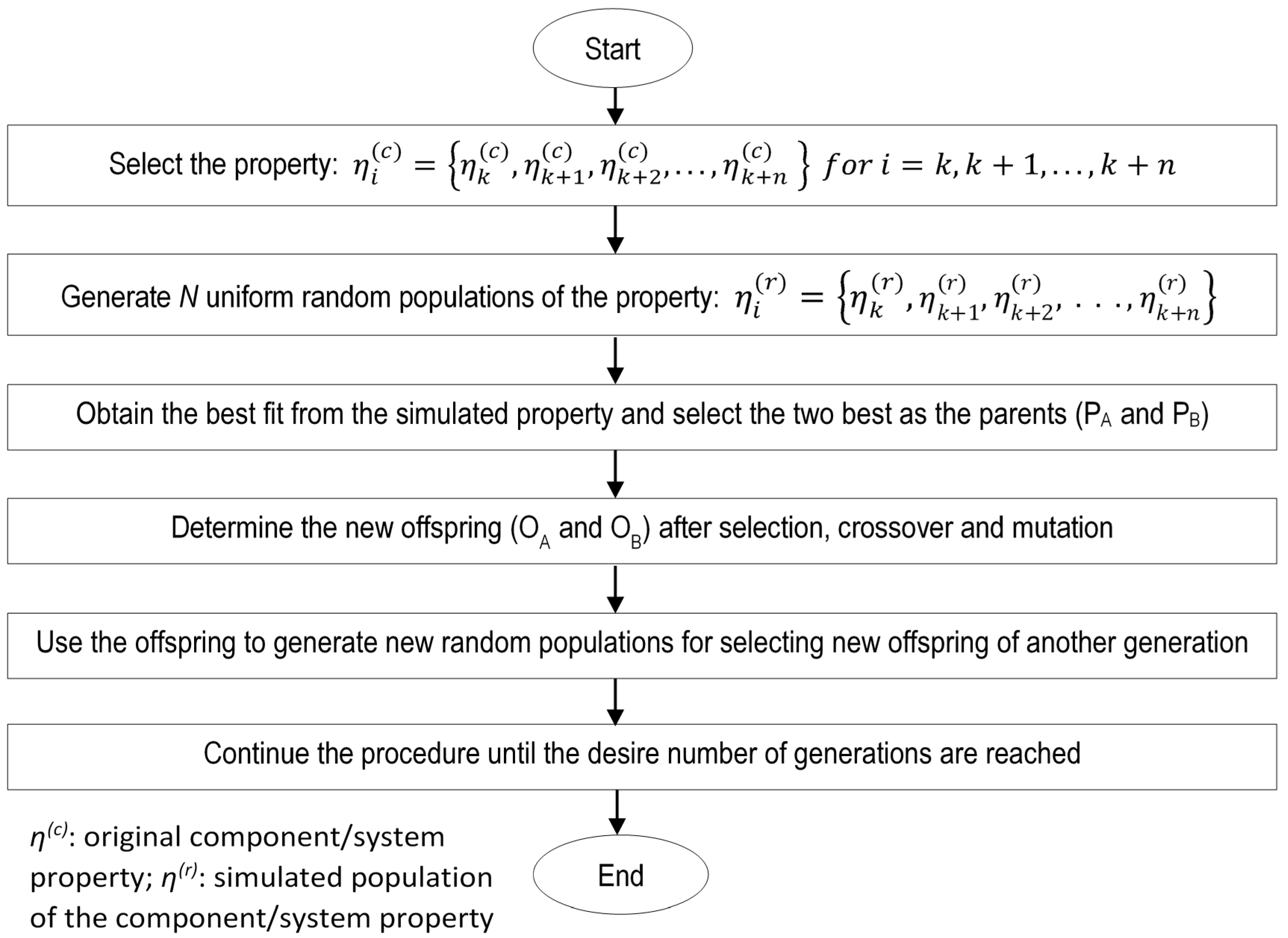
GA is an evolutionary theory technique that employs natural evolution principles to find solutions to natural problems using chromosomes, which represent individual solutions to problems [36,37]. GA has found useful applications in many industrial problems and has been used by numerous authors [38,39,40,41,42,43] in literature for numerous optimization problems; hence, interested readers could consult the references for more insight on the topic. In GA, the arrangement of the discrete constituents of the chromosomes known as genes, give them their unique characteristics; hence, the need for selection, crossover, and mutation in GA to develop new traits of emerging individuals in the solutions of real-world problems. A binary (“1” & “0”) encoding of the chromosomes was used in this work given the successful implementation of the technique by many researchers [36,37]. The process of natural selection in GA requires the picking of the best genes of the chromosomes involved in the evolutionary process and combining them according to a certain proportion (crossover rate). These genes can also be flipped in some special instances (mutation) due to modifications caused by their specific adaptations and environmental constraints. The processes of chromosome selection, gene crossover and mutation are shown in Figure 1.
For the GA to be used for solving optimization problems, many chromosomes are randomly generated from the known parametric values that represent the original or known characteristics of the variable(s) of interest, and two parents (PA and PB), which are the best fit amongst the populations, are selected. The combination of the genes of these parents through a process known as crossover requires the swapping of the genes to form new offspring (OA and OB). The crossover normally occurs at a rate that is sufficient to allow for evolution to occur and can range from 50% to 85% [37]. Since genetic traits can be influenced by environmental conditions, and the passage of time in the evolutionary process, the genes in the chromosomes sometimes develop some new adaptive features via the process of mutation. This procedure (mutation) results in the flipping of the genes from “1” to “0” or vice versa, as shown in OAM and OBM. Considering the influence of time on evolutionary changes, it is possible that the near-ideal characteristics of the chromosomes could be achieved after many generations, hence, helping in the optimization of a given real-life problem. The procedure for using GA to estimate the evolution of C&S characteristics over time is shown in Figure 2. To determine the generation of the GA that will give the OPMPF solution, the estimated values at the generations are subjected to MPF and the best fit result determined by comparison with the original experimental results, using error estimation standards.
4. Illustrative Case Study of Lithium-Ion Battery Charge Capacity Decay
To illustrate the application of GA in OPMPF estimation, and the determination of the RUL of C&S, the charge capacity fade of lithium-ion batteries was used. Three lithium ion (Li+) batteries designated as C#1, C#2 and C#3 were obtained from the database of the Centre for Advanced Lifecycle Engineering (CALCE) of Maryland University [44,45]. The batteries were tested at room temperature using an Airbin BT 2000 battery-testing system with the initial manufacturer-rated capacity of 1.35 Ah. This lithium cobalt oxide (LiCoO2) cathode battery underwent constant charging at the rate of 0.5 C to a voltage of 4.2 V, which was constantly maintained until the current got to 0.05 A. The discharge of the battery also followed the same procedure with a constant discharge current of 0.5 C from 4.2 V to a cutoff voltage of 2.7 V. The estimated charge capacities of the batteries from the experimental results is shown in Figure 3.
4.1. Lithium-Ion Battery Remaining Useful Life (RUL) Estimation
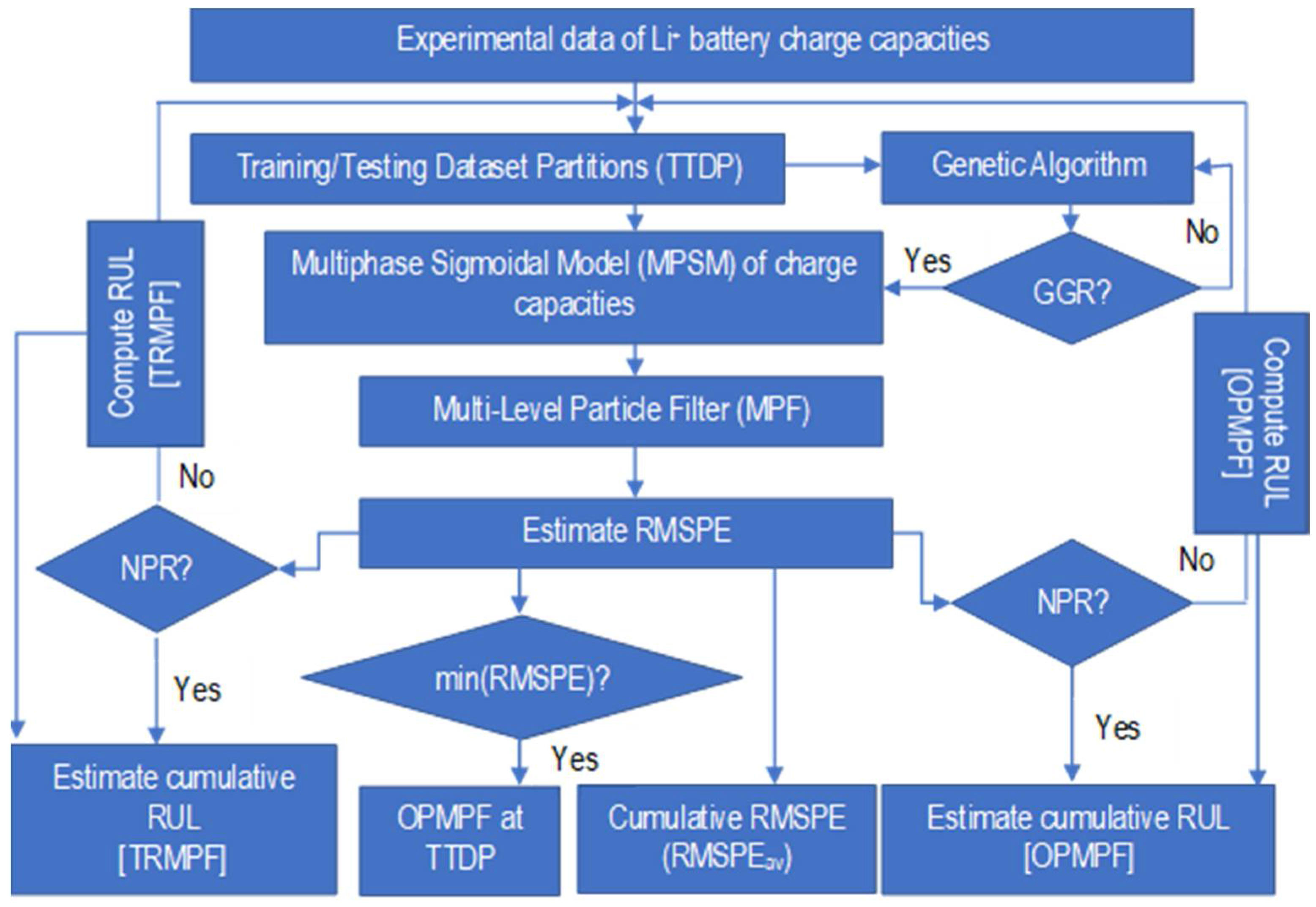
It is very important to note that the TRMPF implemented the MPF procedure for the Li+ batteries’ charge capacities with the original experimental data, whereas GA optimization of the charge capacities at different generations was done prior to MPF in OPMPF estimation. For effective prognosis and RUL estimation with MPF, GA was introduced to determine the optimal generation of the battery charge capacity that will produce the best fit result when compared with the experimental data. To this end, to determine the OPMPF of the Li+ battery charge capacity, GA was used to estimate the evolutionary charge capacities of the batteries at the charging cycles for different generations, and the charge capacities at the generations were subjected to MPF following the procedures described in Section 2.3. The framework used for TRMPF and OPMPF is shown in Figure 4.
In this study, 2000 random uniform values of the charge capacities of the Li+ batteries were generated using the minimum and maximum values of the experimental data of the charge capacities, for each of the charging cycles. This count of the random numbers was used after several trials because it provided the adequate randomization for selecting the values that best fit the charge capacities of the batteries for each of the charging cycles.
For an experimental Li+ battery dataset given by Q(exp)(k) = {Q(exp)(ki), Q(exp)(k2), …, Q(exp)(kns)} obtained at a given experimental charging cycle time ki = {k1, k2, …, kns}, the objective functions {f1, f2, …, fns} of the GA is to obtain the optimal values of the charge capacities for each charging cycle. This was determined using the expression shown in Equation (12):
Here, M represents the number of the randomly generated initial population of the charge capacities of the battery, Q(exp)(k1), Q(exp)(k2), …, Q(exp)(kns) represents the experimental charge capacities of the battery at the different charging cycle, Q(sim)(k1), Q(sim)(k2), …, Q(sim)(kns) represents the simulated value of the charge capacities at the charging cycles, and ns represents the number of charging cycles from which the charge capacities were measured in the charging/discharging experiment.
The optimal solutions obtained at each of the charge capacities helps to select the two parents for crossing. Although several crossover rates could be used as stated previously, 0.70 was adopted because it gave reasonable estimations, and the mutation rate of 0.01 was applied to the evolutionary process. Some researchers have used mutation rates that were as high as 0.2 because of the need to give significant room for evolution, and to prevent chromosomes from being similar [37]. Unfortunately, high values of the mutation rate could result in the introduction of new genetic characteristics that may significantly alter the original traits of the chromosomes, and then result in an excessive evolutionary variation [36]. The crossed chromosomes from the parents result in two offspring with one of them most fitted to the original chromosomes of the experimental battery charge capacity. This offspring is taken as the expected evolutionary generated battery charge capacity at that generation and the charging cycle. To preserve the genetic traits of original chromosomes, the two offspring are used for randomly generating the new population that is used for selecting the next fitted offspring for the succeeding generation. This procedure continues until the expected number of generations of interest is reached.
The optimization for obtaining the OPMPF solution was formulated according to the objective function shown in Equation (13):
Here, Q(exp) is the experimental data of the charge capacities that is expressed as Q(exp) = {Q(exp)(k1), Q(exp) (k2), …, Q(exp)(kns)}and k1, k2, …, kns are the charge cycles at which the charge capacities were obtained, Q(g) represents the charge capacity obtained at the GA generations, ns represents the number of samples of the experimental data, and ng represents the number of generations of the GA under consideration. For this study, the algorithm has been used to obtain 20 generations of the battery charge capacities, which were further used to get the OPMPF by determining the generation with the least root mean square percentage error (RMSPE) after MPF at the various TTDP.
4.2. Decay Trend of GA-Estimated Lithium-Ion Battery Charge Capacity
Before the implementation of MPF, the decay pattern of the GA-estimated battery charge capacities at the generations was determined. This was done with a MPSM that represents a confined exponential decay model shown in Equation (14) because the battery charge capacities decay follows a sigmoidal pattern [27,45,46]:
Here, P1, r1, P2, r2 are model parameters that will be estimated with the battery charge capacities (Q) and k represent the charging cycle.
The model equation is vital for determining the system state equation of the GA obtained charge capacities and gives an initial working guide for estimating the measurement noise in the MPF. The prediction errors of the MPSM, which were determined as the difference between the MPSM and GA-estimated charge capacities at the generations, were used to compute the measurement noises in the MPF. After different trials of various values of the mean absolute errors (MAEs) in the MPF, the best estimates for the measurement noises were obtained as 35% of the MAE for batteries C#1, and C#2, and 50% for battery C#3. This variation in the estimated measurement noises of the batteries could be attributed to the process of the genes’ recombination in the evolution processes at the GA generations.
4.3. Lithium-Ion Battery RUL Estimation
The RUL of the batteries were determined at 80% end-of-life (EOL) threshold by estimating the time it takes to have the initial charge capacity of the batteries depleted to 80% for the various TTDP, using a 9-fold cross-validation ensemble (Figure 5) of the TRMPF and OPMPF. The average of the RUL estimation at the TTDP formed the expected cumulative RUL (RULav) of the batteries as per Equation (15). The fitness of the cross-validation ensemble of the TRMPF and OPMPF were also determined using RMSPE as per Equation (16), and the average RMSPE (RMSPEav) was computed with Equation (17):
Here, Q(mpf), Q(exp), ncv and ns represent TRMPF or OPMPF estimated charge capacities, experimentally determined charge capacity, number of the TTDP and the number of tested samples in the computation, respectively.
5. Results and Discussion
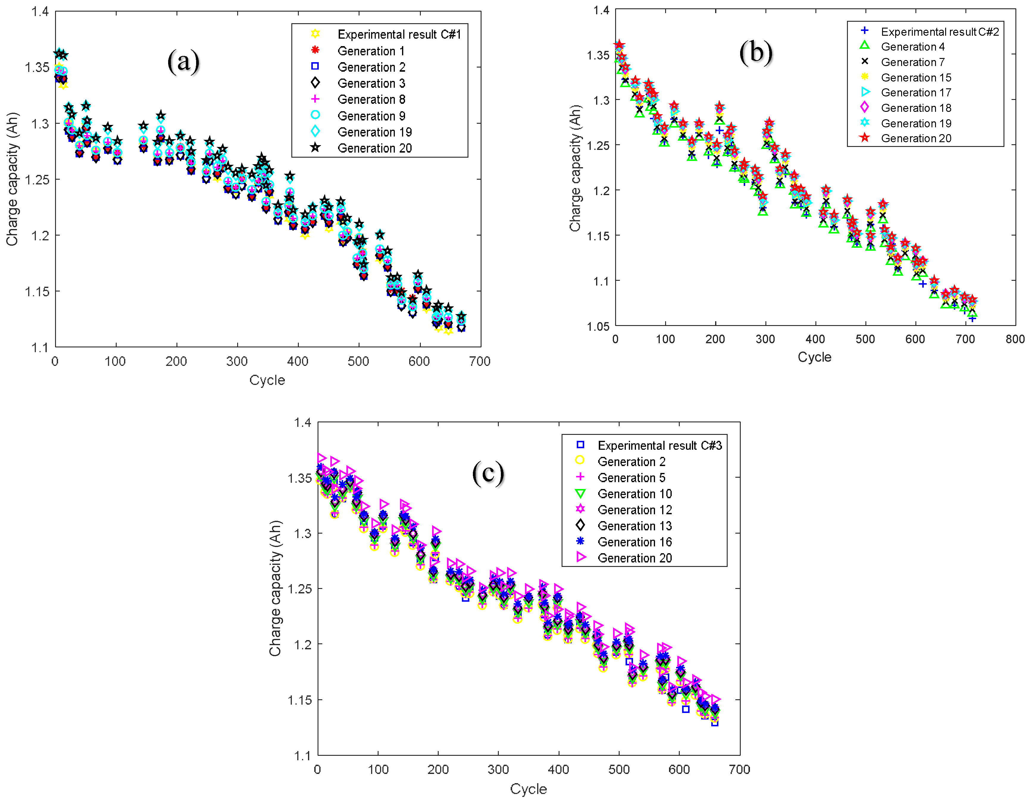
The results obtained from the GA of the three Li+ battery charge capacities for some of the GA generations for the 80% training and 20% testing dataset partition (80:20 TTDP) is shown in Figure 6. The difference between the GA estimations of the charge capacities at the various generations and the experimental results of the datasets were determined with mean absolute error (MAE) and mean absolute percentage error (MAPE), and are shown in Table 1. The small difference between the GA values of the charge capacities and the original experimental results (<1.2%) is a good indication of the high precision of the study technique. Lithium-ion battery C#3 charge capacities were determined with the highest accuracy level with MAPE of between 0.79% and 0.85% followed by battery C#1 with MAPE of 1.02% to 1.08%, whereas battery C#2 has a MAPE of between 1.09% to 1.17%.
The MPF estimations of some of the GA generations shown in Figure 7 give an indication of the correlation of the original experimental dataset with the MPF of the GA generations at 80:20 TTDP. The figures also show that battery C#3 has a higher prediction accuracy with a smaller difference between the MPF and the experimental dataset compared to batteries C#1 and C#2. This is further substantiated by the difference between the MPF-estimated charge capacities and the experimental results per Table 2.
The GA generation, which gave the best fit value of the charge capacities for the testing dataset at the TTDP, was used as the optimal value for estimating the RUL at the OPMPF (see Table 2). The testing dataset was used for determining the optimal solution because it was not used in the initial training of the model, and will give an unbiased judgement of the trained model’s behavior. Considering the 9-fold cross-validation ensemble in Figure 5, and using Equation (16), the average RMSPE of the OPMPF was obtained for the batteries. The average RMSPE for the TRMPF was also determined at the TTDP after using the experimental data for the RMSPE estimation. The summary of the results of the RMSPE estimated with TRMPF and OPMPF are shown in Table 3. It is important to note that the difference between the battery charge capacities obtained at the various TTDP was consistently lower for the OPMPF than the TRMPF. This is an indication of the immense importance of the GA in the optimization of the Li+ battery charge capacities. From Table 3, the RMSPE of battery C#1 obtained by TRMPF is 6.3 times more than that obtained by OPMPF while batteries C#2 and C#3 have the RMSPE obtained by the TRMPF as 3.08 times and 7.33 times, respectively, higher than those obtained by the OPMPF.
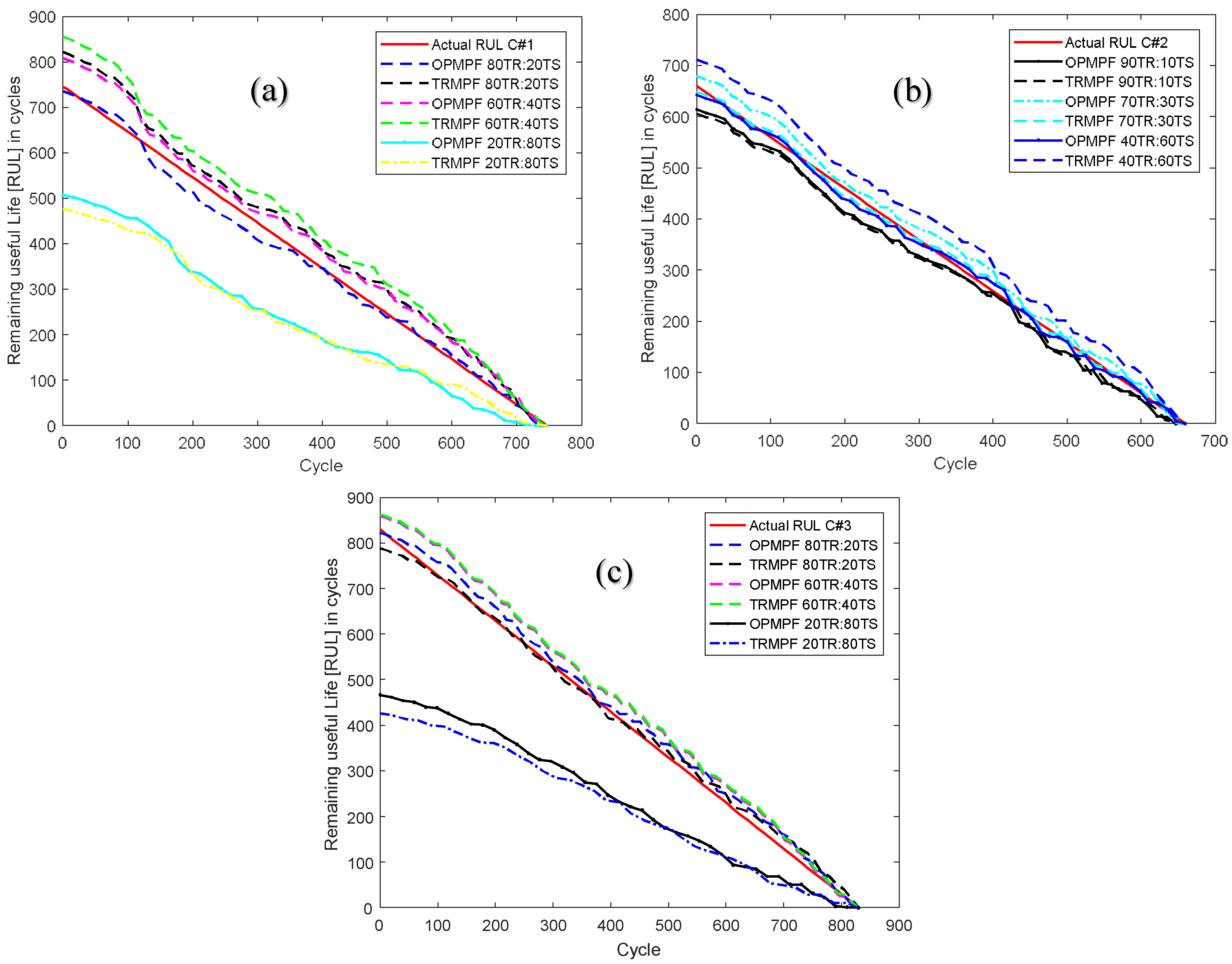
The variation of the RUL of the batteries determined with the OPMPF and TRMPF for some of the TTDP is shown in Figure 8. The figures show that the greater the training dataset, the closer the determined RUL of the batteries to the ideal values because of the enhanced fitting. To avoid an overfitting problem, the cross-validation ensemble that considered training and testing partitions from lower values to higher ones was necessary; hence the estimation of the RUL as the average values of the individual RUL results at the TTDP, as per Table 4. The information in the table, which depicts the mean RUL of the batteries and the difference between the RUL obtained with TRMPF and OPMPF, indicates the superiority of the OPMPF values over the TRMPF estimates. The better values of the RUL obtained with OPMPF in comparison to those gained with TRMPF, indicates that the evolution of the charge capacities with GA overly influenced the computational results of the MPF. Again, the OPMPF results are highly comparable to most of the PF prognosis results in the literature [46,47,48] because the error inherent in the entire prediction process is minimal judging from the information in Table 4.
6. Conclusions
To better estimate the retained life of C&S, an algorithm that combines MPF and GA optimization was used in an OPMPF to determine the RUL. The study implemented the prognosis and RUL of Li+ batteries by using the charge capacities at the cycling in a TRMPF and OPMPF to predict the capacity fade. The TRMPF was done by using the experimental charge capacities at different charging cycles in a direct MPF at different TTDP, whereas in OPMPF GA helped to optimize the charge capacities at the different generations. The optimized charge capacities at the generations were used for MPF prior to the determination of the expected values.
Three experimental results of Li+ batteries were tested with the technique by implementing a 9-fold cross-validation ensemble that represented a TTDP with training and testing ratios of 10:90, 20:80, 30:70, 40:60, 50:50, 40:60, 30:70, 20:80 and 10:90. At the 80% EOL threshold, the average RMSPE and RUL of the batteries determined with TRMPF were found to be between 8.58~15.51% and 5.08~13.65%, respectively. These values were 4.07~5.60 times and 2.42~2.55 times more than the RMSPE and RUL values of the OPMPF, respectively. The variation in the estimation results of the TRMPF and OPMPF gives a good indication of the superiority of the OPMPF technique over the TRMPF. This advantage, which can be traced to the GA optimization of the charge capacities at the different generations, has helped to enhance the prediction accuracy of MPF that has already been shown to give better predictions of components/systems performance than the particle filter.
It may be important to have the OPMPF technique incorporated into real-time components/systems prognosis architecture since GA optimization has the potential to enhance MPF estimation. The number of generations of the GA can be further improved by increasing the number of GA generations in the optimization framework prior to the MPF to further boost the OPMPF result.
Conflicts of Interest
The authors declare no conflict of interest.
References
- Tahan, M.; Tsoutsanis, E.; Muhammad, M.; Karim, Z.A. Performance-based health monitoring, diagnostics, and prognostics for condition-based maintenance of gas turbines: A review. Appl. Energy 2017, 198, 122–144. [Google Scholar] [CrossRef]
- Finn, J.; Wagner, J.; Bassily, H. Monitoring strategies for a combined cycle electric power generator. Appl. Energy 2010, 87, 2621–2627. [Google Scholar] [CrossRef]
- Dai, J.; Das, D.; Ohadi, M.; Pecht, M. Reliability risk mitigation of free air cooling through prognostics and health management. Appl. Energy 2013, 111, 104–112. [Google Scholar] [CrossRef]
- Dai, J.; Das, D.; Pecht, M. Prognostics-based risk mitigation for telecom equipment under free air cooling conditions. Appl. Energy 2012, 99, 423–429. [Google Scholar] [CrossRef]
- Lei, Y. Introduction and background. In Intelligent Fault Diagnosis and Remaining Useful Life Prediction of Rotating Machinery; Butterworth-Heinemann: Woburn, MA, USA, 2017; pp. 1–16. ISBN 9780128115343. [Google Scholar]
- Arora, P.; White, R.E.; Doyle, M. Capacity fade mechanisms and side reactions in lithium-ion batteries. J. Electrochem. Soc. 1998, 145, 3647–3667. [Google Scholar] [CrossRef]
- Yao, Y.; McDowell, M.T.; Ryu, I.; Wu, H.; Liu, N.; Hu, L.; Nix, W.D.; Cui, Y. Interconnected silicon hollow nanospheres for lithium-ion battery anodes with long cycle life. Nano Lett. 2011, 11, 2949–2954. [Google Scholar] [CrossRef] [PubMed]
- Vetter, J.; Novák, P.; Wagner, M.R.; Veit, C.; Möller, K.C.; Besenhard, J.O.; Winter, M.; Wohlfahrt-Mehrens, M.; Vogler, C.; Hammouche, A. Ageing mechanisms in lithium-ion batteries. J. Power Sources 2005, 147, 269–281. [Google Scholar] [CrossRef]
- Shai, D.; Chen, C.; Pooley, M.; D’Andrade, B.W. Prognostics for the Power Industry. In The Power Grid; Academic Press: New York, NY, USA, 2017; pp. 287–316. ISBN 9780128053218. [Google Scholar]
- Ocak, H.; Loparo, K.A.; Discenzo, F.M. Online tracking of bearing wear using wavelet packet decomposition and probabilistic modeling: A method for bearing prognostics. J. Sound Vib. 2007, 302, 951–961. [Google Scholar] [CrossRef]
- Roemer, M.J.; Ghiocel, D.M.; Rieger, N.F. A Probabilistic Approach to the Diagnosis of Gas Turbine Engine Faults. Cond. Monit. Diagn. Eng. Manag. 1998, 2, 767–776. [Google Scholar]
- Guan, X.; Liu, Y.; Jha, R.; Saxena, A.; Celaya, J.; Geobel, K. Comparison of two probabilistic fatigue damage assessment approaches using prognostic performance metrics. Int. J. Progn. Health Manag. 2011, 1, 005. [Google Scholar]
- Kacprzynski, G.J.; Roemer, M.J.; Modgil, G.; Palladino, A.; Maynard, K. Enhancement of physics-of-failure prognostic models with system level features. In Proceedings of the Aerospace Conference Proceedings, Big Sky, MT, USA, 9–16 March 2002; Volume 6, p. 6. [Google Scholar]
- Mendonça, P.L.; Bonaldi, E.L.; de Oliveira, L.E.L.; Lambert-Torres, G.; da Silva, J.G.B.; da Silva, L.E.B.; Salomon, C.P.; Santana, W.C.; Shinohara, A.H. Detection and modelling of incipient failures in internal combustion engine driven generators using Electrical Signature Analysis. Electr. Power Syst. Res. 2017, 149, 30–45. [Google Scholar] [CrossRef]
- Dong, M. A tutorial on nonlinear time-series data mining in engineering asset health and reliability prediction: Concepts, models, and algorithms. Math. Probl. Eng. 2010, 2010, 175936. [Google Scholar] [CrossRef]
- Tobon-Mejia, D.A.; Medjaher, K.; Zerhouni, N.; Tripot, G. A mixture of gaussians hidden markov model for failure diagnostic and prognostic. In Proceedings of the 2010 IEEE Conference on Automation Science and Engineering (CASE), Toronto, ON, Canada, 21–24 August 2010; pp. 338–343. [Google Scholar]
- Smyth, P. Hidden Markov models for fault detection in dynamic systems. Pattern Recognit. 1994, 27, 149–164. [Google Scholar] [CrossRef]
- Peng, Y.; Dong, M. A hybrid approach of HMM and grey model for age-dependent health prediction of engineering assets. Expert Syst. Appl. 2011, 38, 12946–12953. [Google Scholar] [CrossRef]
- Farrar, C.R.; Worden, K. Structural Health Monitoring: A Machine Learning Perspective; John Wiley & Sons: New York, NY, USA, 2012. [Google Scholar]
- Widodo, A.; Yang, B.S. Machine health prognostics using survival probability and support vector machine. Expert Syst. Appl. 2011, 38, 8430–8437. [Google Scholar] [CrossRef]
- Kim, H.E.; Tan, A.C.; Mathew, J.; Kim, E.Y.; Choi, B.K. Machine Prognostics Based on Health State Estimation Using SVM; Springer: Berlin, Germany, 2008. [Google Scholar]
- Jiang, Y.; Wang, Y.; Wu, Y.; Sun, Q. Fault prognostic of electronics based on optimal multi-order particle filter. Microelectron. Reliab. 2016, 62, 167–177. [Google Scholar] [CrossRef]
- Sbarufatti, C.; Corbetta, M.; Giglio, M.; Cadini, F. Adaptive prognosis of lithium-ion batteries based on the combination of particle filters and radial basis function neural networks. J. Power Sources 2017, 344, 128–140. [Google Scholar] [CrossRef]
- Pan, P.; Schonfeld, D. Visual tracking using high-order particle filtering. IEEE Signal Process. Lett. 2011, 18, 51–54. [Google Scholar] [CrossRef]
- Li, T.; Wang, S.; Shi, J.; Ma, Z. An adaptive-order particle filter for remaining useful life prediction of aviation piston pumps. Chin. J. Aeronaut. 2017. [Google Scholar] [CrossRef]
- Orchard, M.E.; Hevia-Koch, P.; Zhang, B.; Tang, L. Risk measures for particle-filtering-based state-of-charge prognosis in lithium-ion batteries. IEEE Trans. Ind. Electron. 2013, 60, 5260–5269. [Google Scholar] [CrossRef]
- Hu, C.; Jain, G.; Tamirisa, P.; Gorka, T. Method for estimating capacity and predicting remaining useful life of lithium-ion battery. Appl. Energy 2014, 126, 182–189. [Google Scholar] [CrossRef]
- Ray, A.; Tangirala, S. Stochastic modeling of fatigue crack dynamics for on-line failure prognostics. IEEE Trans. Control Syst. Technol. 1996, 4, 443–451. [Google Scholar] [CrossRef]
- Orhan, E. Particle Filtering; Center for Neural Science, University of Rochester: Rochester, NY, USA, 2012; Volume 8. [Google Scholar]
- Tokdar, S.T.; Kass, R.E. Importance sampling: A review. Wiley Interdiscip. Rev. Comput. Stat. 2010, 2, 54–60. [Google Scholar] [CrossRef]
- Geweke, J. Bayesian inference in econometric models using Monte Carlo integration. Econom. J. Econom. Soc. 1986, 57, 1317–1339. [Google Scholar] [CrossRef]
- Liu, J.S.; Chen, R. Sequential Monte Carlo methods for dynamic systems. J. Am. Stat. Assoc. 1998, 93, 1032–1044. [Google Scholar] [CrossRef]
- Schon, T.; Gustafsson, F.; Nordlund, P.J. Marginalized particle filters for mixed linear/nonlinear state-space models. IEEE Trans. Signal Process. 2005, 53, 2279–2289. [Google Scholar] [CrossRef]
- Orchard, M.E.; Vachtsevanos, G.J. A particle-filtering approach for on-line fault diagnosis and failure prognosis. Trans. Inst. Meas. Control 2009, 31, 221–246. [Google Scholar] [CrossRef]
- Xiao, Q.; Fang, Y.; Liu, Q.; Zhou, S. Online machine health prognostics based on modified duration-dependent hidden semi-Markov model and high-order particle filtering. Int. J. Adv. Manuf. Technol. 2017, 94, 1283–1297. [Google Scholar] [CrossRef]
- Alcantar, V.; Ledesma, S.; Aceves, S.M.; Ledesma, E.; Saldana, A. Optimization of type III pressure vessels using genetic algorithm and simulated annealing. Int. J. Hydrogen Energy 2017, 42, 20125–20132. [Google Scholar] [CrossRef]
- Sergeeva, M.; Delahaye, D.; Mancel, C.; Vidosavljevic, A. Dynamic airspace configuration by genetic algorithm. J. Traffic Transp. Eng. 2017, 4, 300–314. [Google Scholar] [CrossRef]
- Tsai, P.W.; Pan, J.S.; Chen, S.M.; Liao, B.Y.; Hao, S.P. Parallel cat swarm optimization. In Proceedings of the 2008 International Conference on Machine Learning and Cybernetics, Kunming, China, 12–15 July 2008; Volume 6, pp. 3328–3333. [Google Scholar]
- Tsai, P.W.; Pan, J.S.; Chen, S.M.; Liao, B.Y. Enhanced parallel cat swarm optimization based on the Taguchi method. Expert Syst. Appl. 2012, 39, 6309–6319. [Google Scholar] [CrossRef]
- Chen, S.M.; Huang, C.M. Generating weighted fuzzy rules from relational database systems for estimating null values using genetic algorithms. IEEE Trans. Fuzzy Syst. 2003, 11, 495–506. [Google Scholar] [CrossRef]
- Chen, S.M.; Kao, P.Y. TAIEX forecasting based on fuzzy time series, particle swarm optimization techniques and support vector machines. Inf. Sci. 2013, 247, 62–71. [Google Scholar] [CrossRef]
- Wang, H. Texture analysis method based on fractional Fourier entropy and fitness-scaling adaptive genetic algorithm for detecting left-sided and right-sided sensorineural hearing loss. Fundam. Inform. 2017, 151, 505–552. [Google Scholar] [CrossRef]
- Lu, S. A note on the weight of inverse complexity in improved hybrid genetic algorithm. J. Med. Syst. 2016, 40, 150. [Google Scholar] [CrossRef] [PubMed]
- He, W.; Williard, N.; Osterman, M.; Pecht, M. Prognostics of lithium-ion batteries based on Dempster–Shafer theory and the Bayesian Monte Carlo method. J. Power Sources 2011, 196, 10314–10321. [Google Scholar] [CrossRef]
- Mo, B.; Yu, J.; Tang, D.; Liu, H. A remaining useful life prediction approach for lithium-ion batteries using Kalman filter and an improved particle filter. In Proceedings of the 2016 IEEE International Conference on Prognostics and Health Management (ICPHM), Ottawa, ON, Canada, 20–22 June 2016; pp. 1–5. [Google Scholar]
- Xing, Y.; Ma, E.W.; Tsui, K.L.; Pecht, M. An ensemble model for predicting the remaining useful performance of lithium-ion batteries. Microelectron. Reliab. 2013, 53, 811–820. [Google Scholar] [CrossRef]
- Saha, B.; Goebel, K. Modeling Li-ion battery capacity depletion in a particle filtering framework. In Proceedings of the Annual Conference of the Prognostics and Health Management Society, San Diego, CA, USA, 27 September–1 October 2009; pp. 2909–2924. [Google Scholar]
- Miao, Q.; Xie, L.; Cui, H.; Liang, W.; Pecht, M. Remaining useful life prediction of lithium-ion battery with unscented particle filter technique. Microelectron. Reliab. 2013, 53, 805–810. [Google Scholar] [CrossRef]
Figure 1.
Chromosomes, genetic arrangement, selection, crossover and mutation procedures in the genetic algorithm (GA): PA and PB represent original parents’ chromosomes; OA and OB are offspring from the parents; OAM and OBM are offspring with mutated genes.
Figure 1.
Chromosomes, genetic arrangement, selection, crossover and mutation procedures in the genetic algorithm (GA): PA and PB represent original parents’ chromosomes; OA and OB are offspring from the parents; OAM and OBM are offspring with mutated genes.

Figure 2.
Procedure for estimating the properties of components and systems (C&S) using the GA.

Figure 3.
Summary of the experimental results of the lithium-ion battery charge capacity.
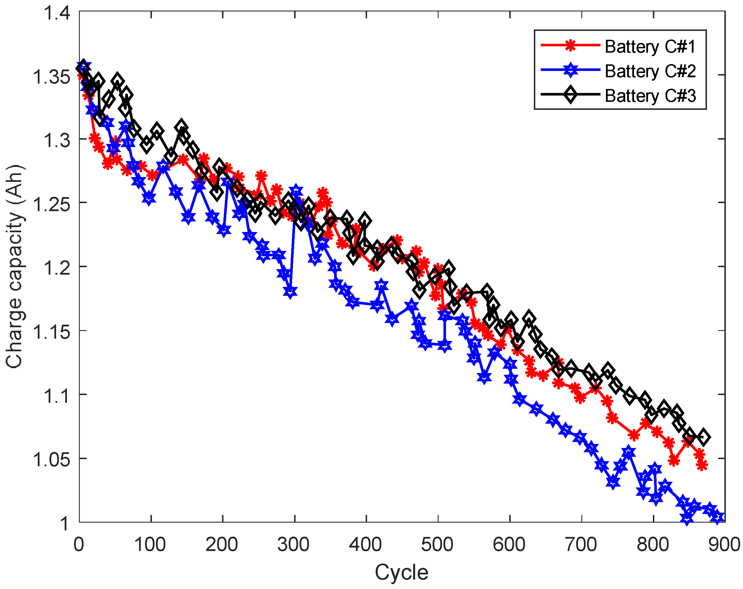
Figure 4.
Optimal multi-level particle filter (OPMPF) procedure and remaining useful life (RUL) estimation of Li+ battery charge capacity decay.
Figure 4.
Optimal multi-level particle filter (OPMPF) procedure and remaining useful life (RUL) estimation of Li+ battery charge capacity decay.

Figure 5.
A 9-fold multi-level particle filter (MPF) cross-validation ensemble used for the computation of the RUL of the lithium-ion batteries at the different training/testing dataset partitions (TTDP).
Figure 5.
A 9-fold multi-level particle filter (MPF) cross-validation ensemble used for the computation of the RUL of the lithium-ion batteries at the different training/testing dataset partitions (TTDP).
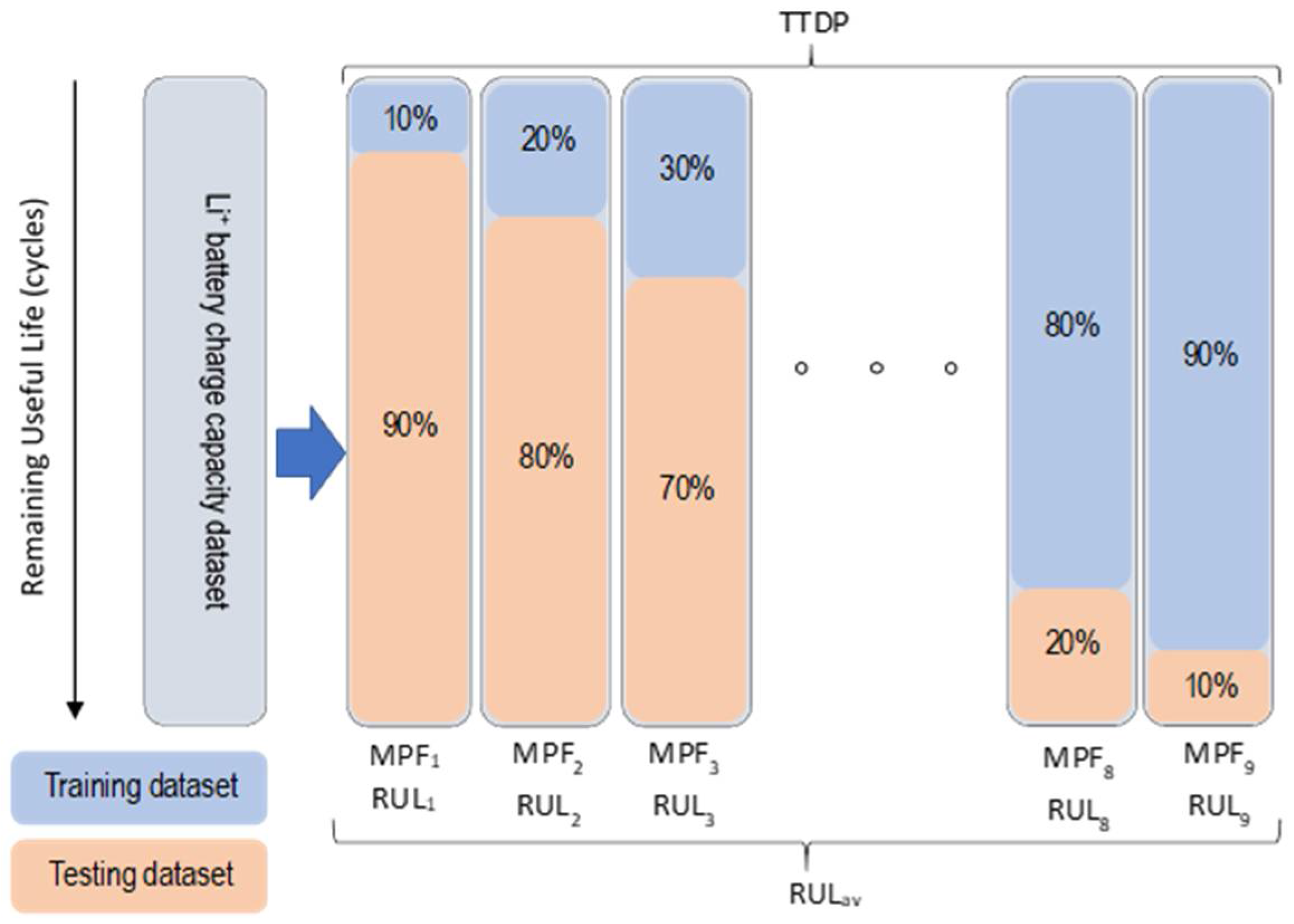
Figure 6.
Comparison of some GA-estimated lithium-ion battery charge capacities with the experimental results for 80:20 TTDP, (a) battery C#1, (b) battery C#2, (c) battery C#3.
Figure 6.
Comparison of some GA-estimated lithium-ion battery charge capacities with the experimental results for 80:20 TTDP, (a) battery C#1, (b) battery C#2, (c) battery C#3.

Figure 7.
Experimental results of the lithium-ion battery charge capacity and some MPF results obtained with the different genetic algorithm generations using 80:20 TTDP, (a) battery C#1, (b) battery C#2, (c) battery C#3.
Figure 7.
Experimental results of the lithium-ion battery charge capacity and some MPF results obtained with the different genetic algorithm generations using 80:20 TTDP, (a) battery C#1, (b) battery C#2, (c) battery C#3.
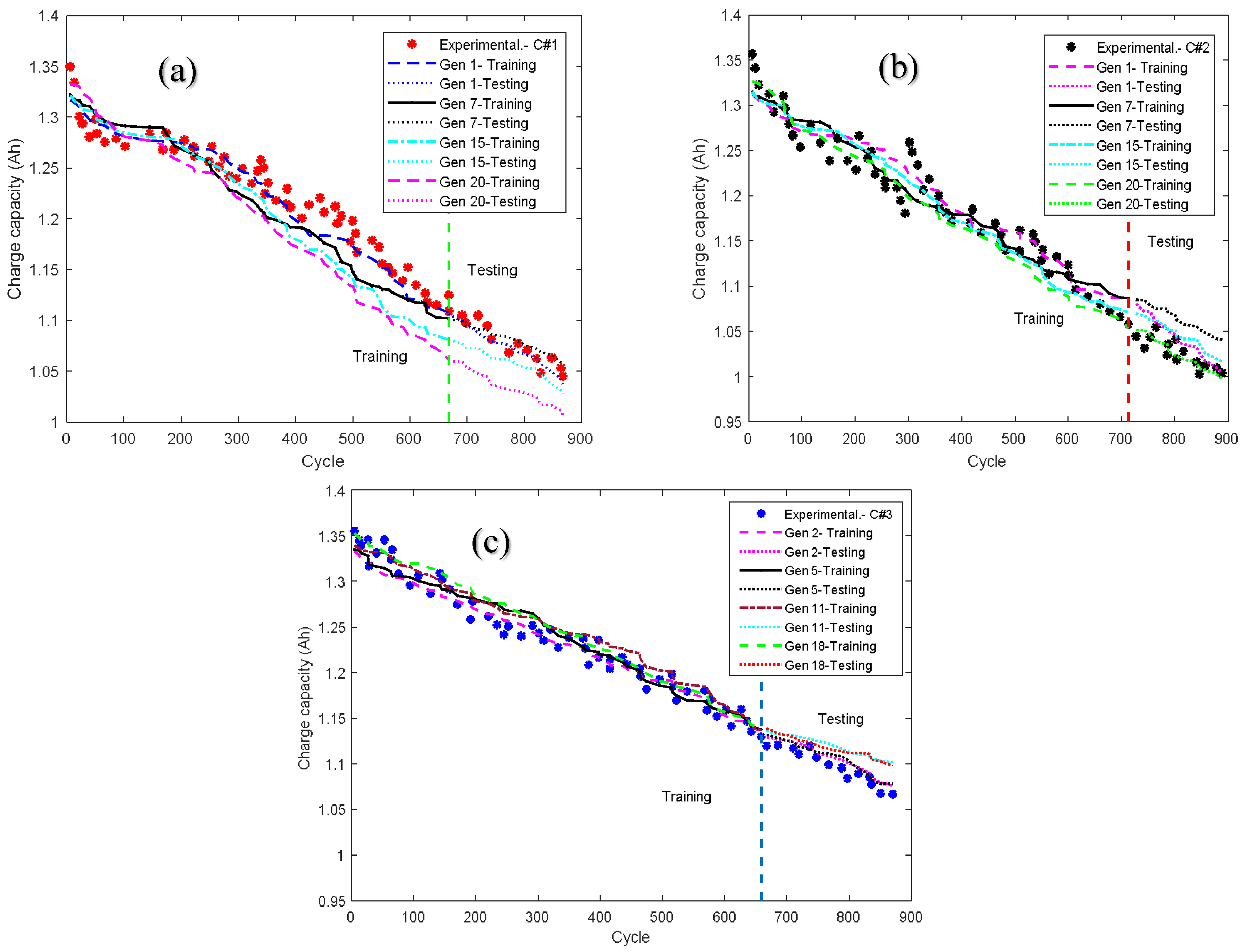
Figure 8.
Alpha–Lambda accuracy plot of the RUL of the Li+ batteries using a combination of some of the TTDP, (a) battery C#1, (b) battery C#2, (c) battery C#3.
Figure 8.
Alpha–Lambda accuracy plot of the RUL of the Li+ batteries using a combination of some of the TTDP, (a) battery C#1, (b) battery C#2, (c) battery C#3.

Table 1.
Summary of the difference between the GA estimated charge capacities and the experimental results as determined with the mean absolute error (MAE) and mean absolute percentage error (MAPE) at the 80:20 TTDP.
Table 1.
Summary of the difference between the GA estimated charge capacities and the experimental results as determined with the mean absolute error (MAE) and mean absolute percentage error (MAPE) at the 80:20 TTDP.
| Genetic Algorithm Generations | Battery C#1 | Battery C#2 | Battery C#3 | |||
|---|---|---|---|---|---|---|
| MAE | MAPE (%) | MAE | MAPE (%) | MAE | MAPE (%) | |
| 1 | 0.012542 | 1.0262 | 0.014126 | 1.1692 | 0.009827 | 0.7885 |
| 2 | 0.012780 | 1.0494 | 0.013663 | 1.1326 | 0.009964 | 0.8084 |
| 3 | 0.012692 | 1.0426 | 0.013521 | 1.1211 | 0.010006 | 0.8123 |
| 4 | 0.012692 | 1.0426 | 0.013590 | 1.1267 | 0.009875 | 0.8022 |
| 5 | 0.012693 | 1.0427 | 0.013614 | 1.1290 | 0.009932 | 0.8066 |
| 6 | 0.012472 | 1.0240 | 0.013190 | 1.0919 | 0.010561 | 0.8568 |
| 7 | 0.012583 | 1.0327 | 0.013432 | 1.1102 | 0.010215 | 0.8281 |
| 8 | 0.012591 | 1.0334 | 0.013410 | 1.1083 | 0.010224 | 0.8287 |
| 9 | 0.012512 | 1.0268 | 0.013429 | 1.1091 | 0.010210 | 0.8275 |
| 10 | 0.012539 | 1.0287 | 0.013446 | 1.1114 | 0.010172 | 0.8243 |
| 11 | 0.012437 | 1.0201 | 0.013350 | 1.1032 | 0.010081 | 0.8158 |
| 12 | 0.012690 | 1.0398 | 0.013484 | 1.1112 | 0.009742 | 0.7879 |
| 13 | 0.012690 | 1.0398 | 0.013478 | 1.1107 | 0.009742 | 0.7879 |
| 14 | 0.012648 | 1.0357 | 0.013847 | 1.1398 | 0.009795 | 0.7907 |
| 15 | 0.012585 | 1.0306 | 0.013723 | 1.1292 | 0.009771 | 0.7888 |
| 16 | 0.012454 | 1.0194 | 0.013779 | 1.1333 | 0.009680 | 0.7812 |
| 17 | 0.012967 | 1.0583 | 0.013960 | 1.1443 | 0.010447 | 0.8396 |
| 18 | 0.013049 | 1.0647 | 0.013625 | 1.1170 | 0.010437 | 0.8389 |
| 19 | 0.013126 | 1.0714 | 0.013863 | 1.1355 | 0.010392 | 0.8352 |
| 20 | 0.013250 | 1.0810 | 0.013605 | 1.1133 | 0.010576 | 0.8499 |
Table 2.
Summary of the difference between the MPF-estimated charge capacities at the GA generations with the experimental data, as measured with the root mean square percentage error (RMSPE) at the 80:20 TTDP.
Table 2.
Summary of the difference between the MPF-estimated charge capacities at the GA generations with the experimental data, as measured with the root mean square percentage error (RMSPE) at the 80:20 TTDP.
| Generations | Battery C#1 | Battery C#2 | Battery C#3 | |||
|---|---|---|---|---|---|---|
| Training | Testing | Training | Testing | Training | Testing | |
| RMPSE (%) | RMPSE (%) | RMPSE (%) | RMPSE (%) | RMPSE (%) | RMPSE (%) | |
| 1 | 1.0119 | 1.4345 | 1.6339 | 2.0210 | 1.2979 | 0.9196 |
| 2 | 2.2817 | 1.7134 | 1.7442 | 1.1866 | 0.9316 | 0.8407 |
| 3 | 2.1552 | 1.0190 * | 1.6275 | 2.9504 | 1.0506 | 2.5433 |
| 4 | 2.9195 | 3.0299 | 1.8242 | 0.9584 * | 0.9463 | 0.7707 |
| 5 | 2.3627 | 2.4592 | 1.6717 | 1.3328 | 1.0331 | 0.9112 |
| 6 | 2.4744 | 2.4617 | 1.6797 | 3.4521 | 1.0659 | 1.8295 |
| 7 | 2.7419 | 1.1883 | 1.6813 | 3.7837 | 0.8799 | 2.8126 |
| 8 | 2.4283 | 2.0409 | 1.5439 | 2.6058 | 1.0385 | 1.8660 |
| 9 | 2.3687 | 1.5284 | 1.5756 | 3.5130 | 1.0959 | 2.7003 |
| 10 | 4.8160 | 5.3376 | 2.7919 | 1.1718 | 1.7588 | 1.0078 |
| 11 | 1.8373 | 1.5030 | 1.7296 | 3.3415 | 1.1747 | 2.1394 |
| 12 | 3.9640 | 4.7354 | 2.0801 | 1.1794 | 1.2603 | 0.6644 |
| 13 | 2.6407 | 1.8496 | 1.7156 | 2.8668 | 1.1547 | 2.1764 |
| 14 | 1.6035 | 1.6166 | 1.8933 | 2.7728 | 1.7223 | 2.2987 |
| 15 | 2.7887 | 2.0031 | 1.6621 | 2.1270 | 1.0690 | 1.6782 |
| 16 | 2.9095 | 4.0364 | 1.6345 | 1.2570 | 1.1555 | 0.4609 |
| 17 | 2.2468 | 2.4977 | 1.6312 | 1.2087 | 1.4299 | 1.1629 |
| 18 | 2.1851 | 1.3490 | 1.6992 | 3.3097 | 1.1238 | 2.0182 |
| 19 | 2.4045 | 2.6096 | 1.7789 | 1.5067 | 1.3861 | 0.7031 * |
| 20 | 3.5188 | 3.9359 | 1.8373 | 0.9990 | 1.3124 | 1.2113 |
Bold *: represents the optimal GA generation, which was considered with respect to the RMSPE of the testing dataset.
Table 3.
Comparison of the RMSPE of the OPMPF and traditional multi-level particle filter (TRMPF) of the batteries.
Table 3.
Comparison of the RMSPE of the OPMPF and traditional multi-level particle filter (TRMPF) of the batteries.
| Training/Testing Dataset Partitions (TTDP) | Battery C#1 | Battery C#2 | Battery C#3 | |||
|---|---|---|---|---|---|---|
| OPMPF | TRMPF | OPMPF | TRMPF | OPMPF | TRMPF | |
| 90:10 | 0.4798 | 9.028 | 1.0752 | 2.3793 | 0.5422 | 9.4759 |
| 80:20 | 1.0191 | 7.4073 | 0.9756 | 2.1281 | 0.4413 | 8.2846 |
| 70:30 | 1.159 | 11.0494 | 1.0518 | 5.7559 | 0.7156 | 11.8412 |
| 60:40 | 1.0437 | 11.8767 | 1.1141 | 9.3161 | 0.652 | 12.6843 |
| 50:50 | 1.2067 | 13.2404 | 1.219 | 8.7671 | 0.8023 | 12.1215 |
| 40:60 | 0.9692 | 13.4266 | 0.9435 | 10.8667 | 1.0859 | 15.5847 |
| 30:70 | 0.8164 | 12.7947 | 1.6497 | 11.3206 | 1.5076 | 17.0099 |
| 20:80 | 7.5976 | 27.6519 | 7.3983 | 12.0204 | 11.8386 | 31.4732 |
| 10:90 | 7.855 | 33.1341 | 9.6566 | 14.6807 | 1.4086 | 20.922 |
| RMSPEav (%) | 2.4607 | 15.5121 | 2.7871 | 8.5817 | 2.1105 | 15.4886 |
| Standard deviation | 2.8224 | 8.2709 | 3.1203 | 4.0882 | 3.4572 | 6.7322 |
Table 4.
End-of-life (EOL) failure cycle for the optimal and traditional particle filters for the batteries.
Table 4.
End-of-life (EOL) failure cycle for the optimal and traditional particle filters for the batteries.
| Experimental Result | ||||||
|---|---|---|---|---|---|---|
| Battery | C#1 | C#2 | C#3 | |||
| 80% EOL failure cycle | 746 | 660 | 830 | |||
| OPMPF and TRMPF predictions RUL at different Training (TR) and Testing (TS) datasets partitions | ||||||
| Training/Testing Dataset Partition (TTDP):TR:TS | C#1 | C#2 | C#3 | |||
| OPMPF | TRMPF | OPMPF | TRMPF | OPMPF | TRMPF | |
| 90:10 | 738 | 630 | 614 | 606 | 822 | 788 |
| 80:20 | 736 | 821 | 626 | 746 | 834 | n/a |
| 70:30 | 824 | 737 | 679 | 649 | 860 | 863 |
| 60:40 | 808 | 856 | 694 | 666 | 835 | n/a |
| 50:50 | 790 | n/a | 700 | 783 | 815 | n/a |
| 40:60 | 789 | n/a | 642 | 711 | 823 | 854 |
| 30:70 | 767 | n/a | 714 | n/a | 830 | n/a |
| 20:80 | 508 | 476 | n/a | n/a | 466 | 426 |
| 10:90 | 539 | 345 | 500 | n/a | n/a | n/a |
| RULav (cycle) | 722 | 644 | 646 | 694 | 786 | 733 |
| Standard deviation | 110 | 184 | 65 | 60 | 121 | 179 |
| Difference | 24 | 102 | 14 | −34 | 44 | 97 |
| % variation | 3.20% | 13.65% | 2.10% | −5.08% | 5.35% | 11.72% |
(n/a means that prediction did not converge, and negative signs show cycle beyond the experimental results).
© 2018 by the author. Licensee MDPI, Basel, Switzerland. This article is an open access article distributed under the terms and conditions of the Creative Commons Attribution (CC BY) license (http://creativecommons.org/licenses/by/4.0/).
Share and Cite
MDPI and ACS Style
Ossai, C.I. Prognosis and Remaining Useful Life Estimation of Lithium-Ion Battery with Optimal Multi-Level Particle Filter and Genetic Algorithm. Batteries 2018, 4, 15. https://doi.org/10.3390/batteries4020015
AMA Style
Ossai CI. Prognosis and Remaining Useful Life Estimation of Lithium-Ion Battery with Optimal Multi-Level Particle Filter and Genetic Algorithm. Batteries. 2018; 4(2):15. https://doi.org/10.3390/batteries4020015
Chicago/Turabian StyleOssai, Chinedu I. 2018. "Prognosis and Remaining Useful Life Estimation of Lithium-Ion Battery with Optimal Multi-Level Particle Filter and Genetic Algorithm" Batteries 4, no. 2: 15. https://doi.org/10.3390/batteries4020015
Note that from the first issue of 2016, this journal uses article numbers instead of page numbers. See further details here.