Development of an Electro-Thermal Model for Electric Vehicles Using a Design of Experiments Approach

Abstract

An accurate and computationally efficient lithium-ion battery model is beneficial when developing state-of-charge (SOC) and state-of-health (SOH) algorithms for battery management systems (BMS). These models allow for software-in-the-loop (SIL) and hardware-in-the-loop (HIL) testing, where the battery pack is simulated in software. However, development of these battery models can be time-consuming, especially when trying to model the effects of temperature and SOC on the equivalent circuit model (ECM) parameters. Estimation of this relationship is often accomplished by carrying out many experiments, which can be costly and time consuming for BMS manufacturers. To address these issues, this paper makes two contributions to literature. First, a comprehensive battery model is developed, where the ECM parameter surface is generated using a design of experiments (DOE) approach. Second, replication runs are conducted to accurately estimate the measurement noise and determine which model parameters are significant. The technique is then compared with existing approaches from the literature, and it is shown that, by using the proposed method, the same degree of accuracy can be obtained while requiring significantly fewer experimental runs. This can be advantageous for BMS manufacturers that require a high-fidelity model but cannot afford to carry out many experiments.

1. Introduction

The rapid depletion of fossil-fuel sources coupled with environmental concerns has resulted in an increased demand for renewable and sustainable energy sources. Lithium-ion (Li-Ion) batteries are emerging as a prominent energy storage device for applications in smart grid and electric vehicles [1]. They have a significant advantage over other battery chemistries, such as lead acid (LA) and nickel metal hydride (NiMH), due to their high efficiency, large energy and power density, and long service life [2,3]. These properties make them ideal for electric vehicles (EVs), plug-in hybrid electric vehicles (PHEVs) and hybrid electric vehicles (HEVs).

Although the popularity of electrified vehicles has increased significantly in the last few years, research is still required to improve the durability, performance and service life of lithium-ion batteries. In addition, safe and reliable control of large battery packs demands a battery management system (BMS) that can accurately predict battery state-of-charge (SOC) and state-of-health (SOH). Improving algorithms on a BMS can be time-consuming, especially if new experiments need to be conducted on each model iteration. In many instances, experimental resources are not available for testing BMS products under various conditions. Therefore, the ability to carry out hardware-in-the-loop (HIL) and software-in-the-loop testing (SIL) is essential.

Development of a HIL and SIL framework requires a high-fidelity and computationally efficient battery model. These models can take a variety of forms from multi-dimensional electro-chemical models to equivalent circuit models (ECM). Electro-chemical models attempt to describe the battery dynamics at the fundamental level using mass and energy balance equations [4,5,6,7,8]. Electrochemical models can be extended to include thermal effects, where the batteries’ thermal response is coupled with its electrochemical behavior [9,10]. These models are governed by a set of ordinary differential equations (ODEs) or partial differential equations (PDEs) and solutions to these systems often require numerical solutions. Therefore, computational time can be a challenge, especially when applied to a battery pack composed of hundreds of cells.

In applications where computational time is an important factor, ECM have been proposed [11,12]. The voltage response under load is captured using a resistor and n number of resistor-capacitor (RC) pairs in series. The value of n is dependent on the application; a larger number of RC pairs will yield a more accurate prediction of the terminal voltage. In addition, the low computational cost of the model is advantageous since it allows for simulation of a realistic battery pack with cell-to-cell variability [13]. It should be noted that the ECM parameters change with temperature, SOC and SOH [14,15]. Therefore, a comprehensive battery simulator should account for these variations when modeling battery dynamics.

The changes in voltage response at different operating temperatures can be adequately captured using coupled electro-thermal models. The temperature dependence on parameters was modeled by Hue et al. [16] using linear spline functions. Lin et al. [17] applied lumped parameter models to cylindrical batteries, where the temperature at the core was predicted. Samadani et al. [18] developed an empirical model for heat generation for application in electric vehicles. Research by Damay et al. [19] explored the extension of these electro-thermal models to include an entropic heat generation term. Low temperature modeling of these batteries has also been carried out by Jaguemont et al. [20].

All of the models described above require a response surface for describing how the ECM parameters change as a function of temperature and SOC. A look-up table or polynomial fit is normally used to develop this surface. However, these approaches require conducting many experiments to fully characterize the surface. In addition, statistical analysis is usually not carried out to determine the measurement noise and estimate which parameters in the model are significant. In light of these gaps in the literature, this paper makes two contributions. First, it proposes a design of experiments (DOE) approach to characterize the ECM parameter model using a minimal number of experiments. Second, the paper carries out an in-depth statistical analysis by conducting center-point experiments to get a more accurate estimate of the noise error variance. The noise error will then be used for conducting hypothesis tests, whereby significant model parameters are identified and retained in the model.

Production and commercialization of a BMS often entails developing an accurate battery model that can be used for HIL and SIL testing. However, investing in model characterization can be expensive since many experiments usually have to be carried out. The goal of this work is to provide future researchers with the tools to quickly develop fast and efficient models, which can in turn be used for improving BMS algorithms for application in EVs.

2. Experimental Procedure

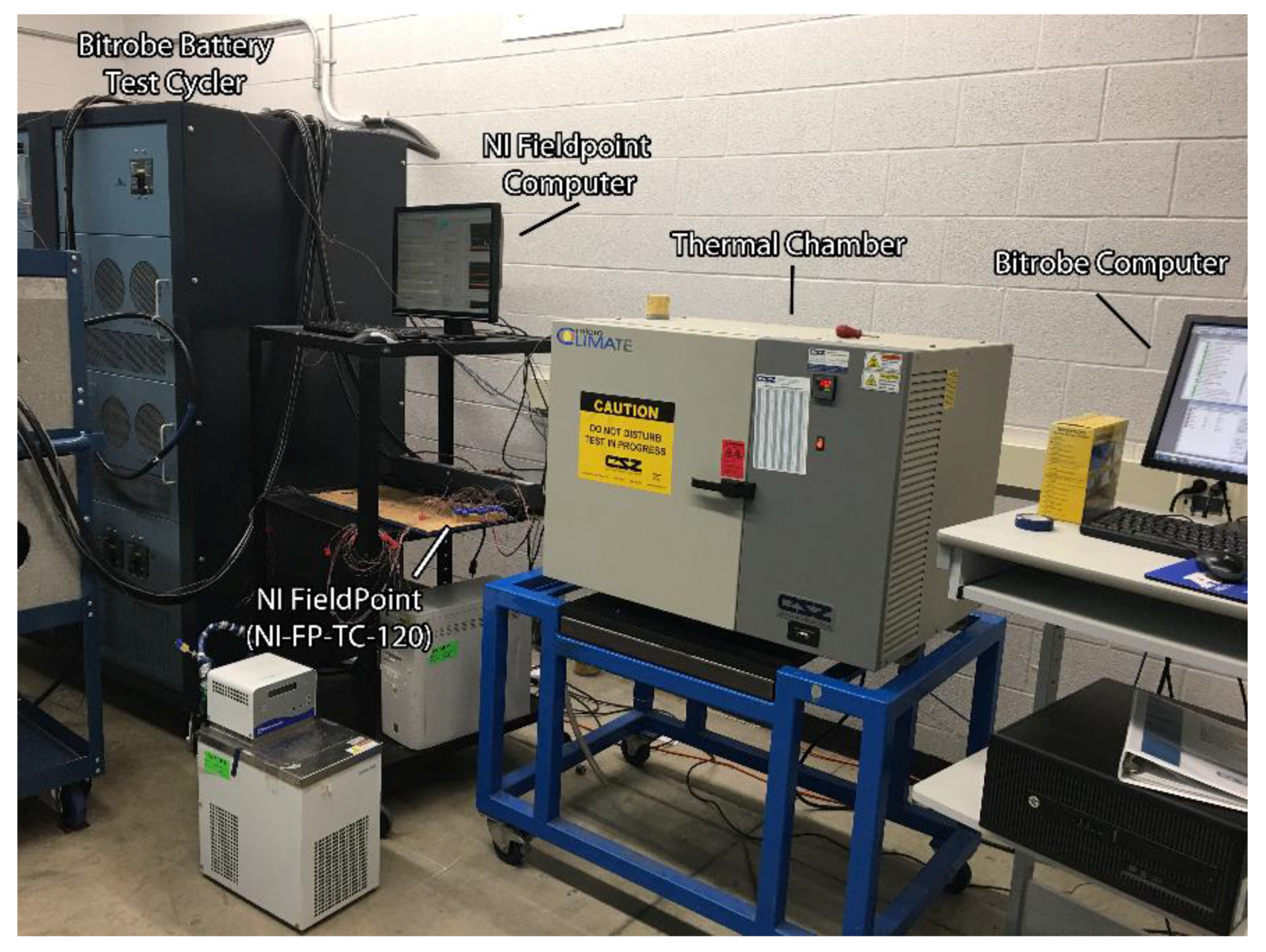
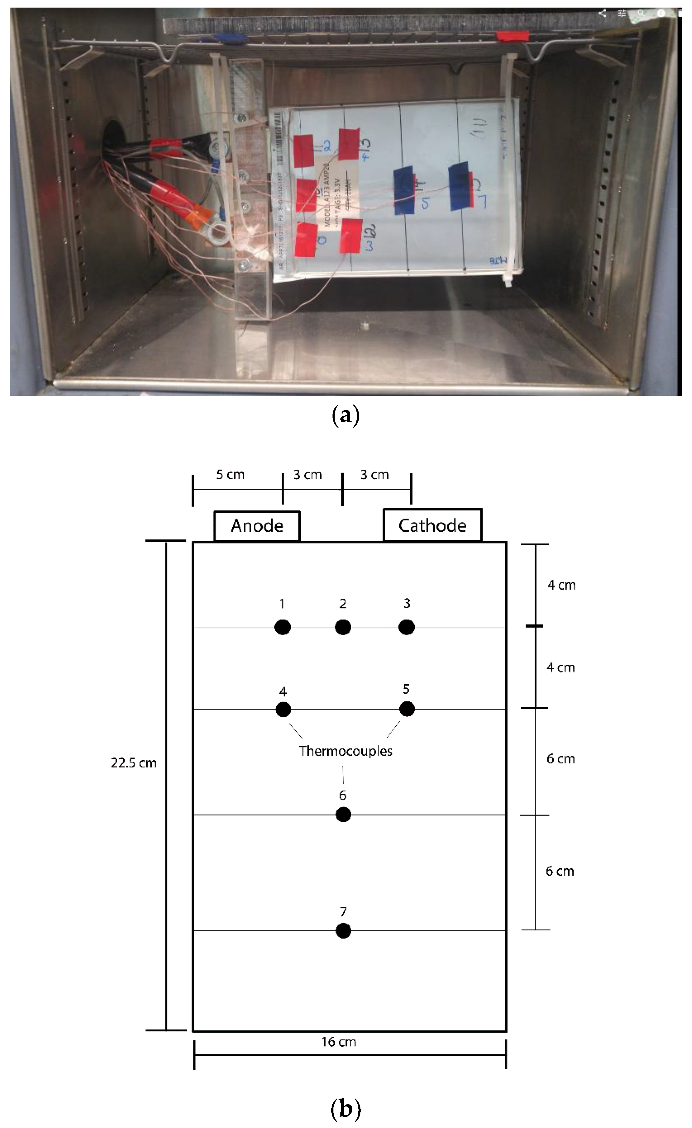
2.1. Experimental Set-Up

All experiments were carried out on a lithium iron phosphate (LFP) battery from A123 systems. The battery specifications are shown in

Table 1. LFP pouch cell specifications.

Parameter	A123 Battery
Cathode Material	LiFePO4
Anode Material	Graphite
Dimension (mm)	7.25 × 160 × 227
Mass (g)	496
Rated Capacity (Ahr)	20
Nominal Voltage (V)	3.3

.

Charging and discharging of the sample cells was carried out using a Bitrode FTV:300/50-20 unit. The cell cycler has an upper voltage limit of 20 V and a maximum current limit of 300 A. The voltage and current measurements were sampled at a frequency of 1 Hz using the VisualCN software. The ambient temperature of the battery was maintained at a constant value using the Cincinnati Sub-Zero Micro Climate unit. The temperature measurements were recorded using the National Instruments (NI) 8-channel thermocouple module at the same sampling frequency as the Bitrode. The experimental set-up is shown in Figure 1.

Seven T-type thermocouples were placed at carefully selected locations within the battery. Preliminary experiments revealed minimal variation in the temperature profile across the battery surface; therefore, the experimental temperature measurements reported in this work will be an averaged value of all seven thermocouple readings. It is also observed that the temperature gradient across the thickness of the cell is negligible; this finding was shown to be true by Mastali et al. [21] for an LFP pouch cell. The specific thermocouple placements are shown in Figure 2. Since the battery temperature is slightly higher close to the tabs, three thermocouples are located at the top portion of the cell, while the rest are distributed across the battery surface to provide a reasonable average battery temperature.

2.2. Cell Characterization Experiments

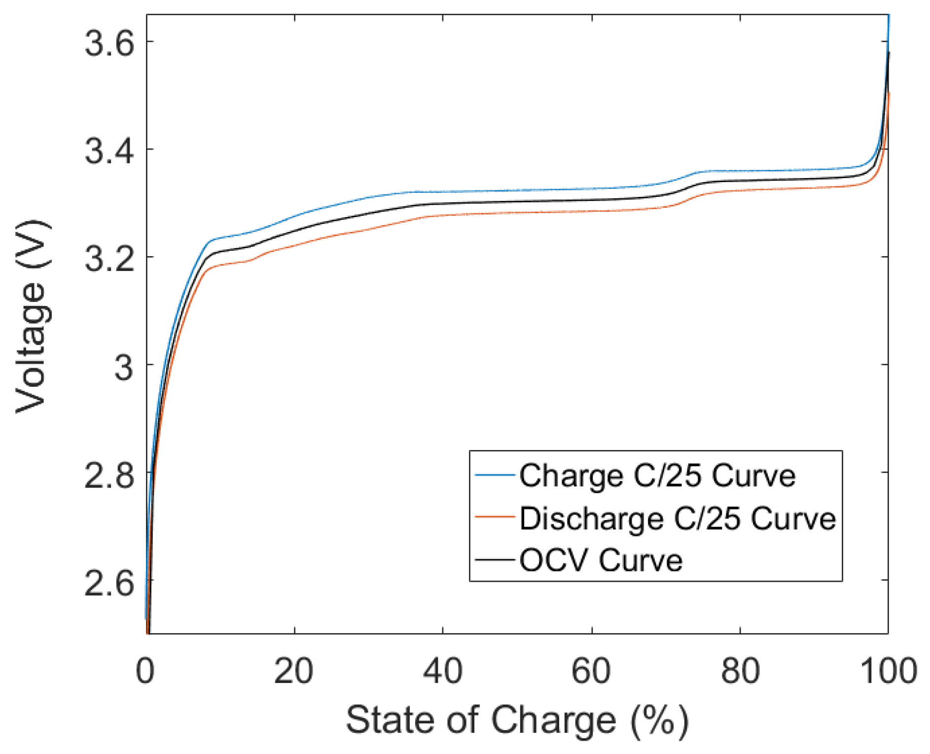
2.2.1. Open Circuit Voltage

The term open circuit voltage (OCV) refers to the voltage measured across the battery when no current is applied. There is a well-established relationship between the OCV and the battery SOC. Development of any model that predicts the voltage response requires estimation of this potential at all SOC points. One approach to determine this curve is to slowly charge and discharge the battery and record the output voltage. The OCV at each SOC is then determined by averaging the charge and discharge voltages. The OCV characterization protocol is as follows:

• Charge the battery to full using a constant current of 1C and maintain the battery at 3.65 V until the current drops to below C/25. This is referred to as constant current constant voltage (CCCV) protocol.
• Allow the battery to rest for an hour.
• Discharge the battery at a constant current of C/25 until the lower limit of 2 V is reached.
• Allow the battery to rest for another hour.
• Charge the battery to full, once again using a constant current of C/25.

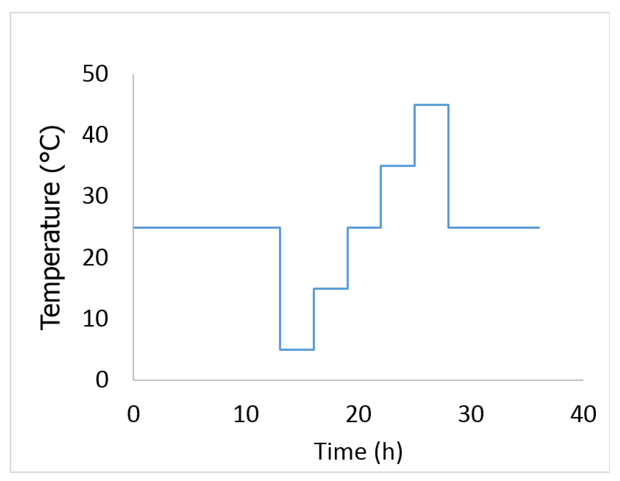
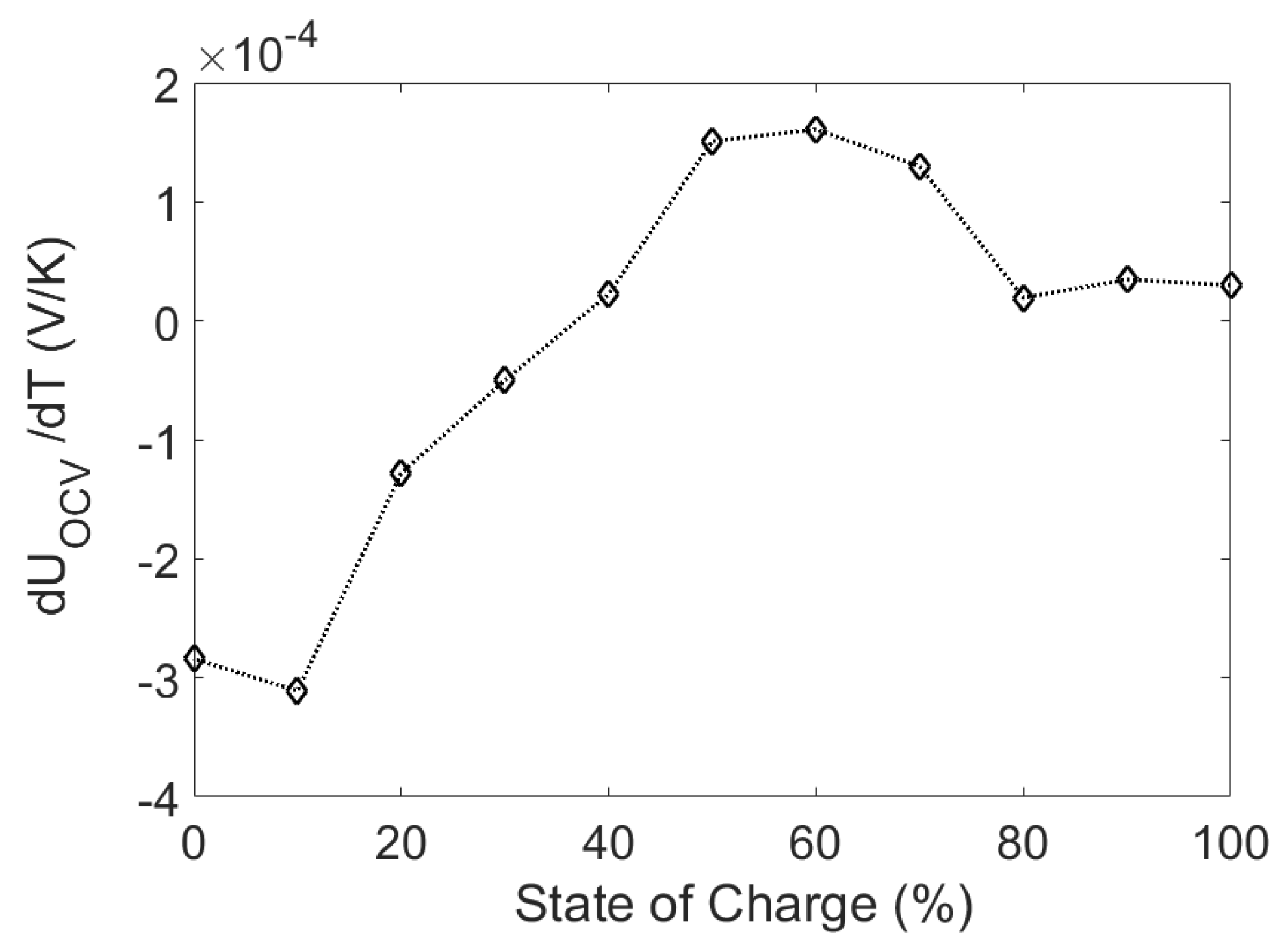
2.2.2. Entropic Heat Generation

The entropic heat generation equation requires calculation of the dU_ocv/dT term for a specific battery chemistry. It should be noted that, regardless of battery geometry and capacity, two batteries with the same chemistry will have similar values of dU_ocv/dT. To determine these values over the range of temperatures, the following experimental procedure was utilized.

• CCCV protocol was used to charge the cell to full.
• For the cell to reach its equilibrium voltage, the battery was rested for a total of 12 h at a constant temperature of 25 °C.
• The battery was then subjected to the temperature profile shown in Figure 3. The cell was assumed to have reached its equilibrium temperature after 3 h of rest.
• The battery was discharged to the next SOC point using a constant current discharge at 1C for 6 min. The cell was assumed to have reached its equilibrium voltage after 12 h of rest. The procedure was repeated until the cell was fully discharged.

Using the above procedure, the value of dU_ocv/dT can be estimated for each specific SOC. These values can then be used in a look-up table to determine the entropic heat generation as the battery is cycled.

2.2.3. Hybrid Pulse Power Characterization Test

Understanding the behavior of ECM parameters under different operating conditions is essential for building a comprehensive battery simulator. Identification of these model parameters can be carried out using the hybrid pulse power characterization (HPPC) test. A brief description of the characterization procedure is shown below:

• At a specific SOC value, discharge the battery at a constant current of 1C for 10 s.
• Allow the battery to rest for 40 s.
• Charge the battery at ¾C for 10 more seconds.

The ECM parameters change with SOC and temperature; therefore, to identify these parameters, the HPPC test needs to be carried out at different temperature and SOC values. Since discharging to a new SOC point or temperature value requires 1–2 hour of rest, characterization of these models can be time consuming. To resolve this issue, a DOE approach will be proposed in the next section, where HPPC runs will be carried out at select temperature and SOC points.

It should be noted that the experiments described above have been previously used when characterizing the battery. The novelty of this paper lies in determining the optimal conditions where the HPPC experiments should be carried out. By using a central composite design (CCD), the goal is to obtain the maximum amount of information about the response surface while using a minimal number of runs.

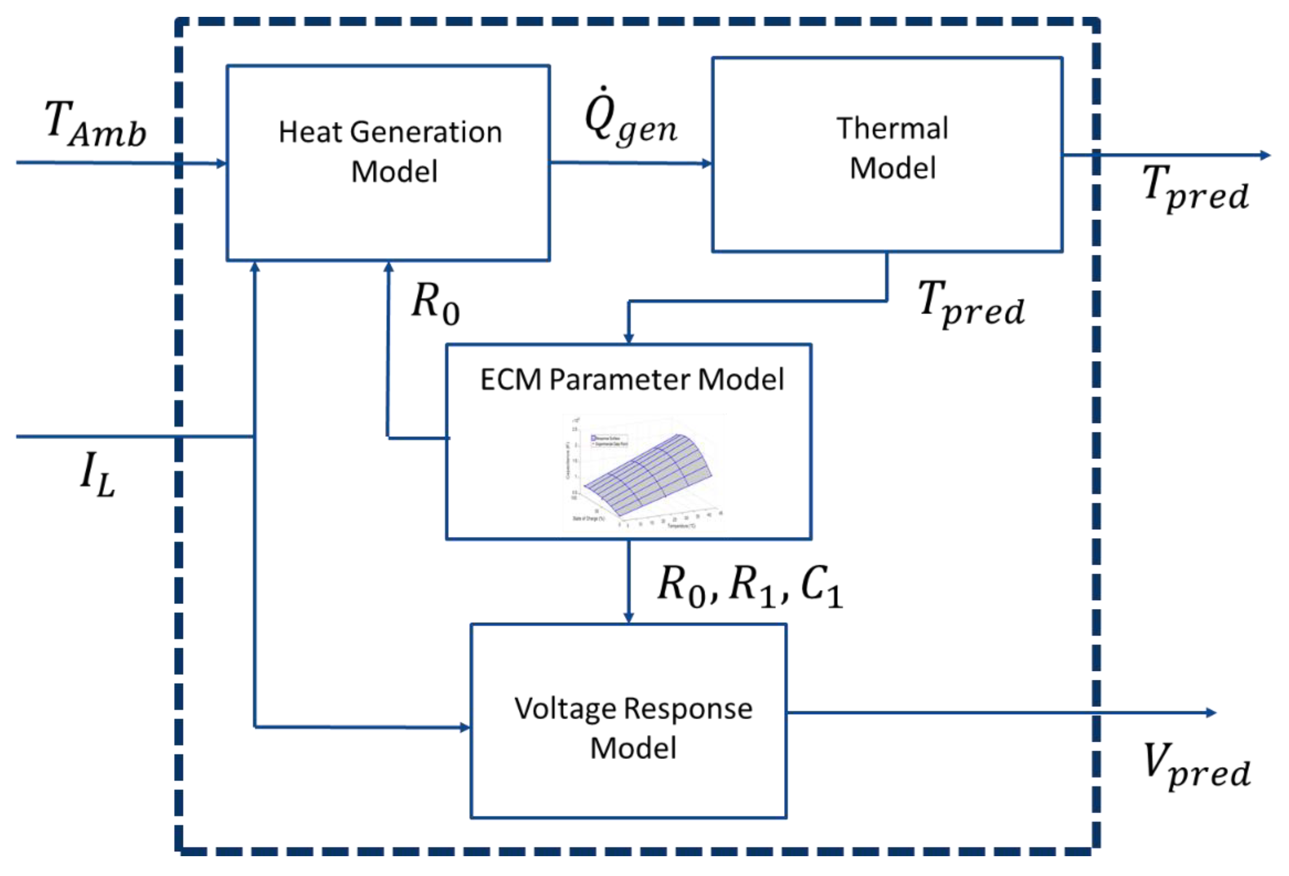
3. Algorithm Development

The voltage and temperature response of the battery can be modeled using four smaller sub-models that are coupled together. A heat generation and thermal model is used to predict the temperature rise within the battery, while a voltage response model is used to estimate the terminal voltage of the battery under load. The models are connected to one another through the ECM parameter model. Figure 4 illustrates these four sub-models and how they are linked to each other.

Figure 4 shows that there are two inputs into the overall model: the ambient temperature and the applied current. Using these variables, the terminal voltage and temperature of the battery is predicted at each time step. It should be noticed in Figure 4 that both voltage and temperature predictions rely on the accuracy of the ECM parameter model. Therefore, accurately determining the response surface for the ECM parameter model is essential for developing a reliable battery simulator.

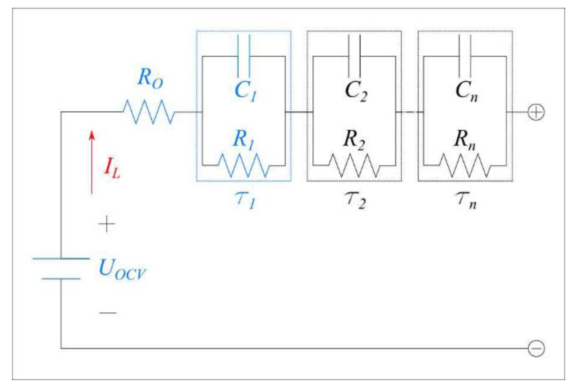
3.1. Voltage Response Sub-Model

The voltage response of a lithium-ion battery can be modeled using the ECM shown in Figure 5.

The ohmic resistor, represented by R_o, accounts for the electrical ionic resistance in the current collector, electrode, electrolyte and battery tabs. It represents the instantaneous drop in voltage observed when a current is initially applied to the battery. In addition to this drop, the battery’s voltage changes as a function of time due to polarization effect. This dynamic behavior is modeled using the resistor-capacitor pairs shown in Figure 5. The first RC pair, with a time constant τ₁, represents the polarization resulting from the interfacial charge-transfer reactions at the electrode. The second RC pair, with a longer time constant τ₂, is used to represent the polarization resistances due to concentration related effects. Additional RC pairs can be added to improve the predictive capability of the model at the expense of computational time. Finally, the open circuit voltage represents the thermodynamic potential in the battery when no current is flowing.

This paper will use a first order ECM with one RC pair. The electrical elements used in the model are highlighted in blue in Figure 5 and the governing equations are shown below.

$$\frac{d\left(U_{th}\right)}{dt}=-\frac{U_{th}}{R_1{C}_1}+\frac{I_L}{C_1}$$

(1)

$$U_L=U_{ocv}-U_{th}-I_L{R}_o$$

(2)

It should be noted that the current is positive during discharge and negative during charge. Since the OCV is a function of the battery’s SOC, the voltage response model needs an accurate estimate of the battery’s SOC. The SOC can be determined by integrating the current flowing through the battery and the coulomb counting equation is shown below.

$$SO{C}_b=SO{C}_0-\frac{1}{C_n}{{\displaystyle \int }}^{\text{}}\frac{I_{}{}_L}{3600}dt$$

(3)

where SOC_b is the battery SOC at a given time step, I_L,k is the current at the time step, C_n is the battery capacity and SOC₀ is the initial SOC. The algorithm requires an initial SOC value, and it is assumed that no measurement error is present in the current for the duration of the test.

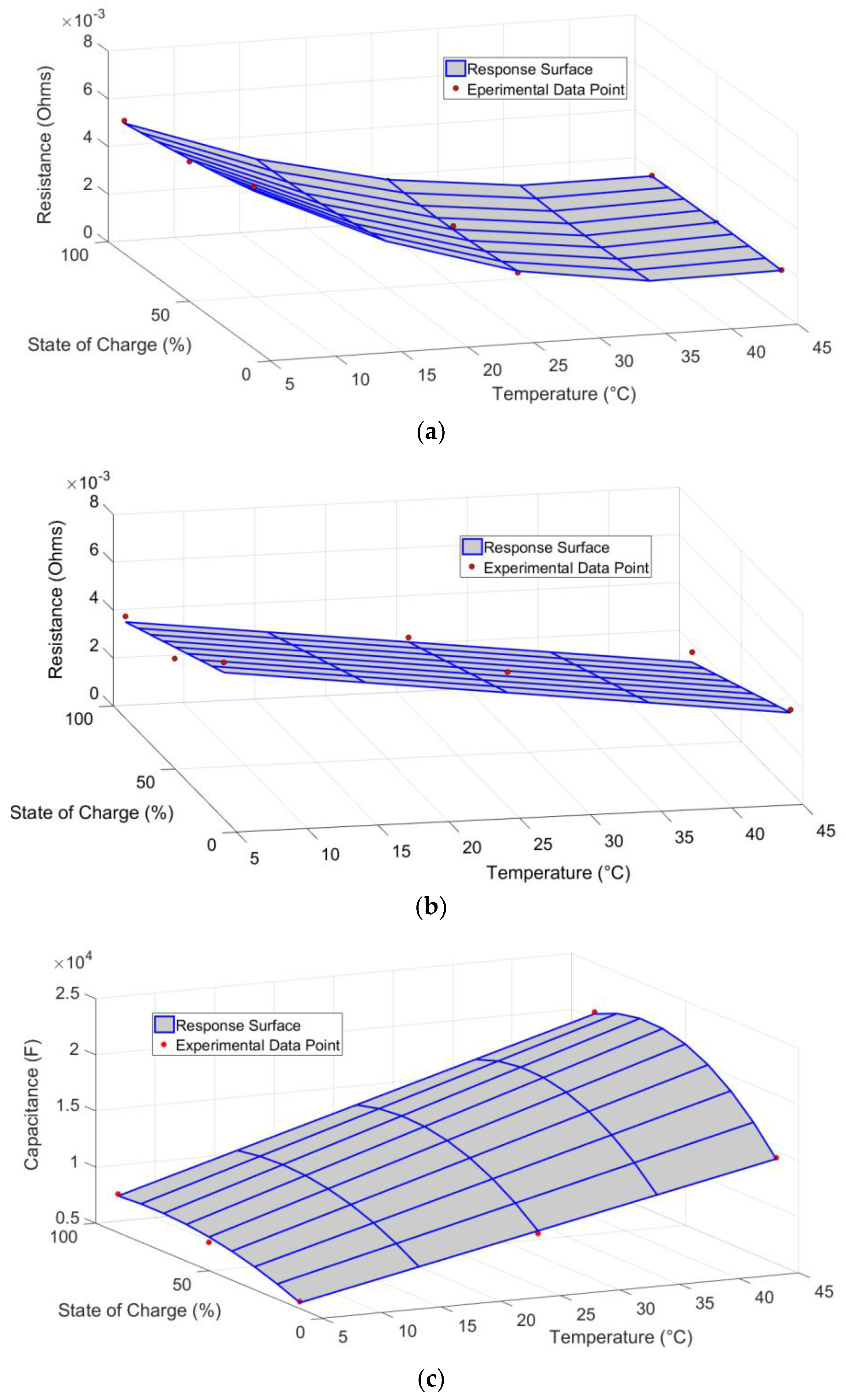
3.2. ECM Parameter Sub-Model

As previously mentioned in Section 1, the temperature and SOC dependence on the model parameters is usually described using a two-dimensional look-up table. This approach is time consuming, however, as the accuracy of the look-up table is dependent on the size of the grid. Many tests need to be carried out to accurately model the region between sampling points. This is especially true if an additional, third, variable such as SOH is included in the modeling approach. Therefore, this work proposes a DOE approach in developing the empirical model, where experiments are only conducted at optimal points. Although the design in this work only considers battery temperature and SOC, the proposed framework could be easily extended to include battery SOH in future works.

When designing an experiment with multiple independent variables or factors, it is important to vary the factors simultaneously instead of one at a time. This type of strategy is referred to as factorial design and has been applied to various applications [22]. One type of factorial design is 2^k, where the experiments are selected at the high and low levels of each factor. For example, suppose one is interested in studying the effect of temperature on the response, where the temperature values range between 5 °C and 45 °C. The high level refers to running the experiment at 45 °C, while the low level refers to carrying the test out at 5 °C. The model regression coefficients, obtained using this design, can be shown to have minimum variance [23]. The 2^k factorial design can be used to fit the following first-order empirical model.

$$y={\beta }_0+{\beta }_1{x}_1+{\beta }_2{x}_2+{\beta }_3{x}_1{x}_2+\epsilon$$

(4)

It should be noted that the first-order model shown above is only accurate if the response surface is a plane. Since ECM parameter response can be highly non-linear with respect to temperature and SOC [17], a more advanced model is required to account for this curvature. Therefore, this paper uses a face-centered CCD, shown in Figure 6, for developing the response surface.

In Figure 6, the corner points, shown in red, represent the 2^k design. The levels of the two factors are shown in coded form, where the values of −1 and +1 represent the min and max of each individual variable and the value of zero represents the mid-point of the two levels. Since 2^k designs cannot accurately account for non-linear trends, additional star points (shown in blue) can be added to the experimental design. The value of these star points, represented by α, can range from ±1 for face-centered CCD to ±1.414 for rotatable CCD. In this paper, a face-centered CCD is utilized, resulting in the star points at ±1. Finally, using this design, a second-order empirical model can be fitted, and is shown in Equation (5). For a more in-depth analysis on experimental design, please refer to the review written by Candioti et al. [24].

$$y={\beta }_0+{\beta }_1{x}_1+{\beta }_2{x}_2+{\beta }_3{x}_1{x}_2+{\beta }_4{x}_1{}^2+{\beta }_5{x}_2{}^2+{\beta }_6{x}_1{x}_2{}^2+{\beta }_7{x}_1{}^2{x}_2+{\beta }_8{x}_1{}^2{x}_2{}^2+\epsilon$$

(5)

With regards to operational limits, since it is difficult to get precise HPPC curves when the battery is close to empty or full, the maximum and minimum value of battery SOC are taken as 90% and 10%, respectively. The temperature range for this work is between 45 °C and 5 °C. Using the operating range, the experimental conditions for the corner and star points can be determined (

Table 2. Experimentally designed conditions for the HPPC test used in developing the ECM parameter surface.

Type	Temperature (°C)	SOC (%)
Corner and Star Points	5	10
	5	50
	5	90
	25	10
	25	50
	25	90
	45	10
	45	50
	45	90
Replicate Run	25	50
	25	50
	25	50
	25	50
	25	50

).

In addition to the star and corner points shown in Figure 6, center points need to be carried out to get an estimate of the measurement noise. In this work, five HPPC experiments were carried out at the middle temperature of 25 °C and middle SOC of 50%. To ensure that the experiments are true replicates, the battery was brought to the same equilibrium point for each run. Measurement error can be obtained by finding the standard deviation of the estimated parameters, R₀, R₁, and C. The equation for standard deviation is shown below:

$$s_{p.e}^2=\frac{{\left(X_{i,rep}-{\overline{X}}_{rep}\right)}^2}{N_{rep}-1}$$

(6)

where X_i,rep represents the obtained parameter value, ${\overline{X}}_{rep}$ is the average parameter value and N is the total number of runs. In the literature, where a statistical analysis has been carried out on the parameters, it is often common practice to use the mean squared error (MSE) to obtain an estimate of the noise variance [17]. This assumption is only valid, however, if the model is assumed to fit the data perfectly and the residuals are found to contain only noise. Using replicate runs would allow for a more accurate estimation of the noise variance, which can then be used to determine if the parameters in the model are significant. Finally, based on the experimental procedure described in Section 2, the hybrid pulse power characterization test was conducted at the following test points.

Developing the ECM parameter model presents a two-level regression approach. First, a non-linear regression analysis needs to be carried out on the HPPC test to identify the circuit parameters at the different operating conditions. Next, a second-order empirical model is used to describe how the ECM parameters change with temperature and SOC. The second-order empirical model is shown below:

$$\begin{gathered} Parameter={\beta }_0+{\beta }_1{\mathrm{T}}_c+{\beta }_{2}SO{C}_b+{\beta }_3{\mathrm{T}}_c^2+{\beta }_{4}SO{C}_b^2+{\beta }_5\left({\mathrm{T}}_c\times SO{C}_b\right)+{\beta }_6({\mathrm{T}}_c^2 \\ \times SO{C}_b)+{\beta }_7\left(SO{C}_b^2\times {\mathrm{T}}_c\right)+{\beta }_8\left({\mathrm{T}}_c^2\times SO{C}_b^2\right) \end{gathered}$$

(7)

where T_c represents the surface temperature of the cell. The results from the empirical model are described in Section 4.2 and the developed model is incorporated into the comprehensive model.

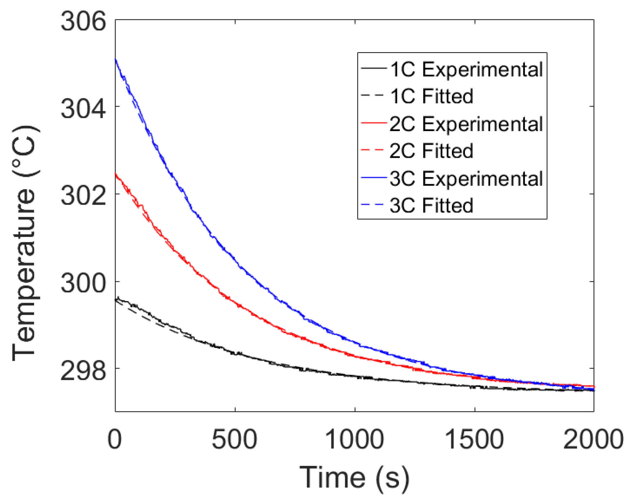
3.3. Thermal Response Sub-Model

Predicting the battery temperature first requires carrying out an energy balance around the cell. The energy balance reveals that the change in the battery’s internal energy is equal to the amount of heat generated within the cell minus the heat lost to the environment.

$$m_c{C}_p\frac{d{T}_c}{dt}={\dot{Q}}_{gen}-hA\left(T_c-T_{\infty }\right)$$

(8)

where $m$_c is the mass of the cell, C_p is the specific heat capacity, $T_{\infty }$ is the ambient temperature, h is the overall heat transfer coefficient and A is the area across which heat transfer occurs. The terms on the left-hand side of the equation describe the change in temperature of the cell, while the other two terms represent the heat generated within the cell and heat transferred to the environment. It is assumed in this study that heat loss through the current-carrying wires as well as the radiation from the surface of the cell is incorporated within the overall heat transfer coefficient.

Application of the above equation first requires determining the overall heat transfer coefficient within the cell. The value of this constant depends on the thermal chamber parameters and is assumed to be constant throughout this experiment. The heat transfer coefficient can be estimated using the above equation in situations where no heat generation is present. This occurs when there is no current following through the cell, so the above equations can be simplified as follows:

$${{\displaystyle \int }}_{T_0}^{T_f}\frac{d{T}_c}{-T_c+T_{\infty }}={{\displaystyle \int }}_0^{t_{rest}}\left(\frac{hA}{m_c{C}_p}\right)dt$$

(9)

where T_f is the final temperature after the rest period, T₀ is the initial temperature, t_rest is the total time of rest and $\frac{hA}{m_c{C}_p}$ is a constant that depends on the cell parameters. Assuming $\frac{hA}{m_c{C}_p}=\propto$, the cell temperature during the rest period can be modeled as:

$$T_c=T_{\infty }+\left(T_o-T_{\infty }\right)e^{-\propto t_{rest}}$$

(10)

The value of α can be estimated by first cycling the cell until it reaches a higher than ambient temperature. The cell is then allowed to cool and the measured temperature can be used to estimate the value of α.

In addition to the heat transfer coefficient, the heat generated within the cell also needs to be quantified. The heat produced is the result of two terms, shown in the equation below [25,26,27].

$${\dot{Q}}_{gen}=R_o{I}_L^2-I_L{T}_c\frac{d{U}_{OCV}}{d{T}_c}$$

(11)

The first term on the right-hand side of Equation (11) represents the irreversible heat generation due to the internal resistance of the battery. The value of R₀ is obtained from the ECM parameter model and is found to change with temperature and SOC. The second term represents the reversible heat generation, also known as entropic heat. Depending on the current direction and the battery’s SOC, the value of this term can be either negative or positive. The experimental procedure for determining dU_ocv/dT_c is described in Section 2 and the results are summarized in Section 4.

4. Results and Discussion

The following section examines the battery characterization results from the OCV curve, the heat generation model and the thermal model. The experimental data obtained from the DOE approach is utilized to develop a response surface that is a function of temperature and SOC. Replication runs are conducted and analyzed to estimate the measurement noise. This noise estimate is then used to determine which parameters in the response surface are significant. The developed surface is incorporated into the electro-thermal model and compared against the experimental values. Finally, the predictive capability of the proposed response surface is compared with currently existing approaches from the literature.

4.1. Cell Characterization Results

The OCV of the battery was determined by performing the procedure outlined in Section 2.1. The results are shown in Figure 7.

The deviation between the charge and discharge curve is a result of two factors. First, although the current is small, a voltage drop will be observed during the charge and discharge cycle due to the internal resistance of the battery. Second, battery hysteresis has been documented before in LFP batteries, and this effect is clearly visible in Figure 7. For the purposes of this work, the hysteresis will not be modeled, and will be left as future work.

The entropic heat generation experiments, described in Section 2.2.2, were carried out for the LFP battery. The work done by Jalkanen et al. [28] presents a more detailed analysis of how the dU_ocv/dT_c curve can be obtained. The results obtained in this work for LFP are shown below.

By examining Figure 8, it is evident that the value of the entropic heat generation term can be either positive or negative depending on the SOC of the battery. Therefore, incorporation of this term in the heat generation model can provide more accurate prediction results. It should be noted that the curve shown above can be used for any LFP chemistry, regardless of capacity or geometry.

Finally, cooling curves can be generated for the current experimental set-up. The LFP cell, which was initially at 0% SOC, was charged to 100% SOC and allowed to rest for an hour. The heat lost to the environment was measured during the resting period, and the measured temperature values were used to estimate the heat transfer coefficient using Equation (10). The results are provided in Figure 9.

Upon fitting the thermal model to the experimental data during the rest period, an average value of 0.00175 s⁻¹ was observed for α. Figure 9 shows good agreement between model and experiment providing further confidence in the estimated value of the heat transfer coefficient.

4.2. ECM Parameter Results

The hybrid pulse power characterization test was carried out at the experimental conditions shown in Table 2. The HPPC test was used to extract the battery impedance parameters at different operating conditions. The non-linear model shown in Equations (1) and (2) can be used in the identification procedure, where the parameter values are obtained by minimizing the mean sum of squared error.

$$\min \left({\displaystyle \sum }_{i=1}^n{\left(U_{L,i}-U_{exp}\right)}^2\right)$$

(12)

where U_L,i represents the model voltage and U_exp is the experimental voltage. The parameter identification procedure was executed in MATLAB using the Levenberg–Maruardt non-linear least squares method.

The estimated battery impedance parameters will then be used as dependent variables in the second regression model. Since the second-order model, shown in Equation (7), is linear in the parameters, linear regression approaches can be utilized. It should be noted that three different response surfaces were generated in this work, one for each ECM parameter. The following equation can be used to find the parameters in the second-order model.

$$\widehat{\beta }={\left(X^{T}X\right)}^{-1}{X}^{T}y$$

(13)

where $\widehat{\beta }$ represents the estimated parameters, $X$ represents the design matrix based on the independent variables and $y$ represents the response variable. In addition to the parameters, the standard error of each individual parameter can be obtained using the equation below.

$$S.E\left(\widehat{\beta }\right)=\sqrt{{\left(X^{T}X\right)}_{ii}^{-1}\ast s_{p.e}^2}$$

(14)

where $s_{p.e}^2$ is the pooled error variance for each specific parameter, determined using center point runs. Using the proposed regression approach, the center point runs can first be analyzed to determine the measurement error for each of the three response surfaces. The values are shown in

Table 3. The measurement error for the ECM parameters surfaces.

ECM Parameters	Measurement Error
Ohmic Resistance (Ohms)	1.88 × 10−5
Thevenin Resistance (Ohms)	5.02 × 10−4
Thevenin Capacitance (F)	2.18 × 102

.

By examining Table 3, it is evident that, although both the ohmic and Thevenin resistance values are in the same order of magnitude, the variance for estimating the Thevenin resistance is substantially higher than the ohmic resistance. Therefore, accurate analysis of how the ECM parameters change with temperature and SOC requires consideration of the noise error. Failure to do so would result in incorrect conclusions about which effects are significant.

Once an estimate of the noise error is obtained, the next step is to determine which parameters in the second order model are significant. A hypothesis test was conducted at a confidence level of 95% to determine if any of the model parameters could be removed. The p-values are shown in

Table 4. Empirical model parameters for the change in R₀, R₁ and C as a function of temperature and SOC.

Ohmic Resistance Response Surface
Type	Parameter Estimate	Standard Error	p-Value
Intercept	2.39 × 10−3	1.88 × 10−5	<0.0001
Temp	−2.06 × 10−3	1.33 × 10−5	<0.0001
SOC	−7.14 × 10−5	1.33 × 10−5	0.0058
Temp2	1.43 × 10−3	2.30 × 10−5	<0.0001
SOC2	−1.93 × 10−5	2.30 × 10−5	0.448
Temp × SOC	2.93 × 10−4	9.38 × 10−6	<0.0001
Temp2 × SOC	−2.48 × 10−4	1.62 × 10−5	0.0001
SOC2 × Temp	−1.58 × 10−4	1.62 × 10−5	0.0006
SOC2 × Temp2	1.77 × 10−4	2.81 × 10−5	0.0032
Thevenin Resistance Response Surface
Type	Parameter Estimate	Standard Error	p-Value
Intercept	3.00 × 10−3	5.02 × 10−4	0.0039
Temp	−1.35 × 10−3	3.55 × 10−4	0.0191
SOC	−1.38 × 10−3	3.55 × 10−4	0.0175
Temp2	2.63 × 10−4	6.14 × 10−4	0.4893
SOC2	1.20 × 10−3	6.14 × 10−4	0.1222
Temp × SOC	1.18 × 10−4	2.51 × 10−4	0.6637
Temp2 × SOC	3.53 × 10−4	4.34 × 10−4	0.4620
SOC2 × Temp	−9.91 × 10−5	4.34 × 10−4	0.8305
SOC2 × Temp2	−4.94 × 10−4	7.53 × 10−4	0.5475
Thevenin Capacitance Response Surface
Type	Parameter Estimate	Standard Error	p-Value
Intercept	1.41 × 104	2.18 × 102	<0.0001
Temp	6.27 × 103	1.54 × 102	<0.0001
SOC	2.16 × 103	1.54 × 102	0.0002
Temp2	−2.88 × 102	2.67 × 102	0.3409
SOC2	−2.22 × 103	2.67 × 102	0.0011
Temp × SOC	8.51 × 102	1.09 × 102	0.0015
Temp2 × SOC	7.99 × 10	1.89 × 102	0.6943
SOC2 × Temp	−1.04 × 103	1.89 × 102	0.0052
SOC2 × Temp2	7.35 × 102	3.27 × 102	0.0879

, where a value below 0.025 means that the estimated parameter is significant.

Table 4 shows that, for the ohmic resistance response surface, all parameters except for SOC² were found to be significant. The results reveal that the temperature has a significant effect on the ohmic resistance and second order quadratic terms are required to adequately capture this trend. This significant temperature effect stems from the fact that the battery transport properties such as ionic diffusion in electrode particles are highly temperature dependent. There are also significant interaction effects between temperature and SOC, which translates to saying that the effect of SOC on the ohmic resistance is dependent on the temperature.

The parameters for the Thevenin resistance empirical model were found to only contain linear temperature and SOC terms. As temperature and SOC decrease, the Thevenin resistance was found to increase in a linear fashion. Finally, the capacitance was found to change with both temperature and SOC, where a decrease in temperature was found to decrease the Thevenin capacitance. The parameters that were found to be insignificant can be removed and the remaining parameters can be re-estimated. These parameter values are summarized in

Table 5. The final parameter values for the response surface of ohmic resistance, Thevenin resistance and Thevenin capacitance.

Ohmic Resistance		Thevenin Resistance		Thevenin Capacitance
Intercept	8.39 × 10−3	Intercept	6.76 × 10−3	Intercept	3.75× 103
Temp	−3.35 × 10−4	Temp	−7.07 × 10−5	Temp	1.71 × 102
SOC	−1.93 × 10−5	SOC	−2.63 × 10−5	SOC	7.60 × 10
Temp2	4.16 × 10−6			SOC2	−4.74 × 10−1
Temp × SOC	2.24 × 10−9			Temp × SOC	5.25 × 100
Temp2 × SOC	1.04 × 10−8			SOC2 × Temp	−4.19 × 10−2
SOC2 × Temp	1.02 × 10−8
SOC2 × Temp2	−2.40 × 10−10

.

The values obtained can be used to generate the response surface and the graphs are shown below.

Figure 10 shows good agreement between the model output and the experimental data points. The ohmic resistance and Thevenin capacitance surfaces contain a good amount of curvature and therefore a second-order model is required for these parameters. The Thevenin resistance, on the other hand, only requires a linear model in temperature and SOC. Although it is possible that other correlations are present for this parameter, they cannot be statistically identified due to the higher measurement noise that was present when estimating the Thevenin resistance. Therefore, the results reveal the importance of carrying out a thorough statistical analysis before any conclusions are made.

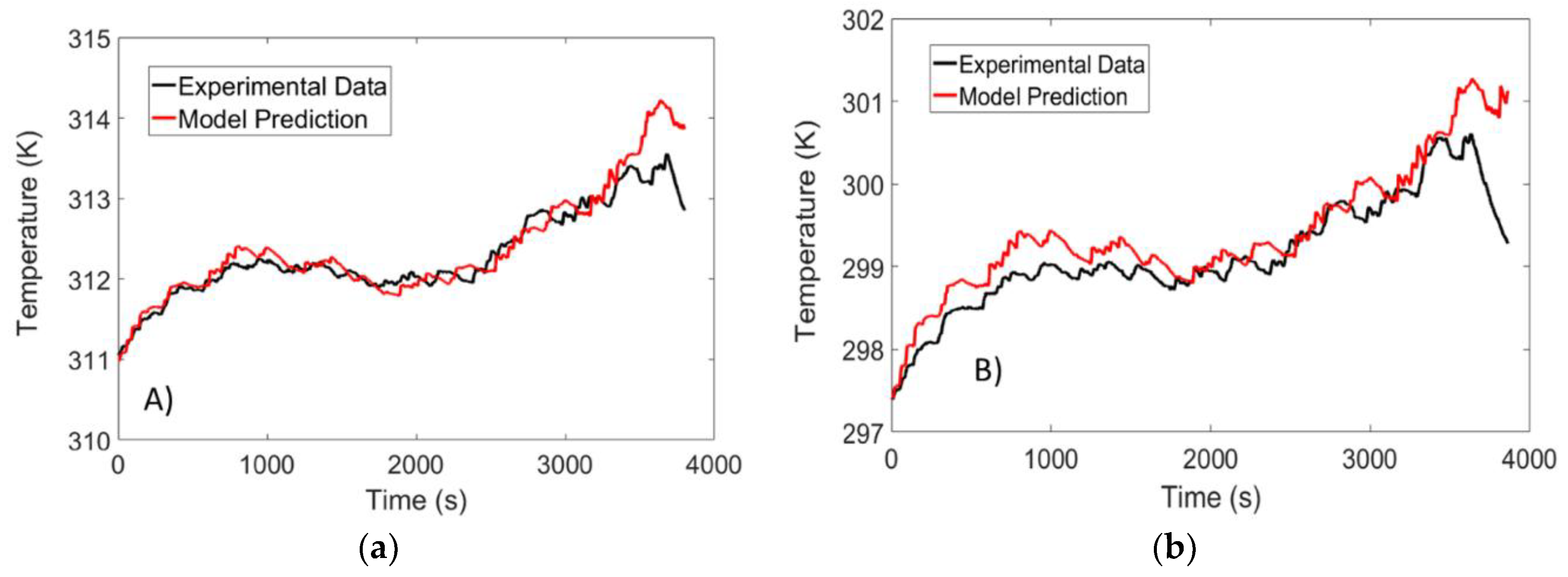
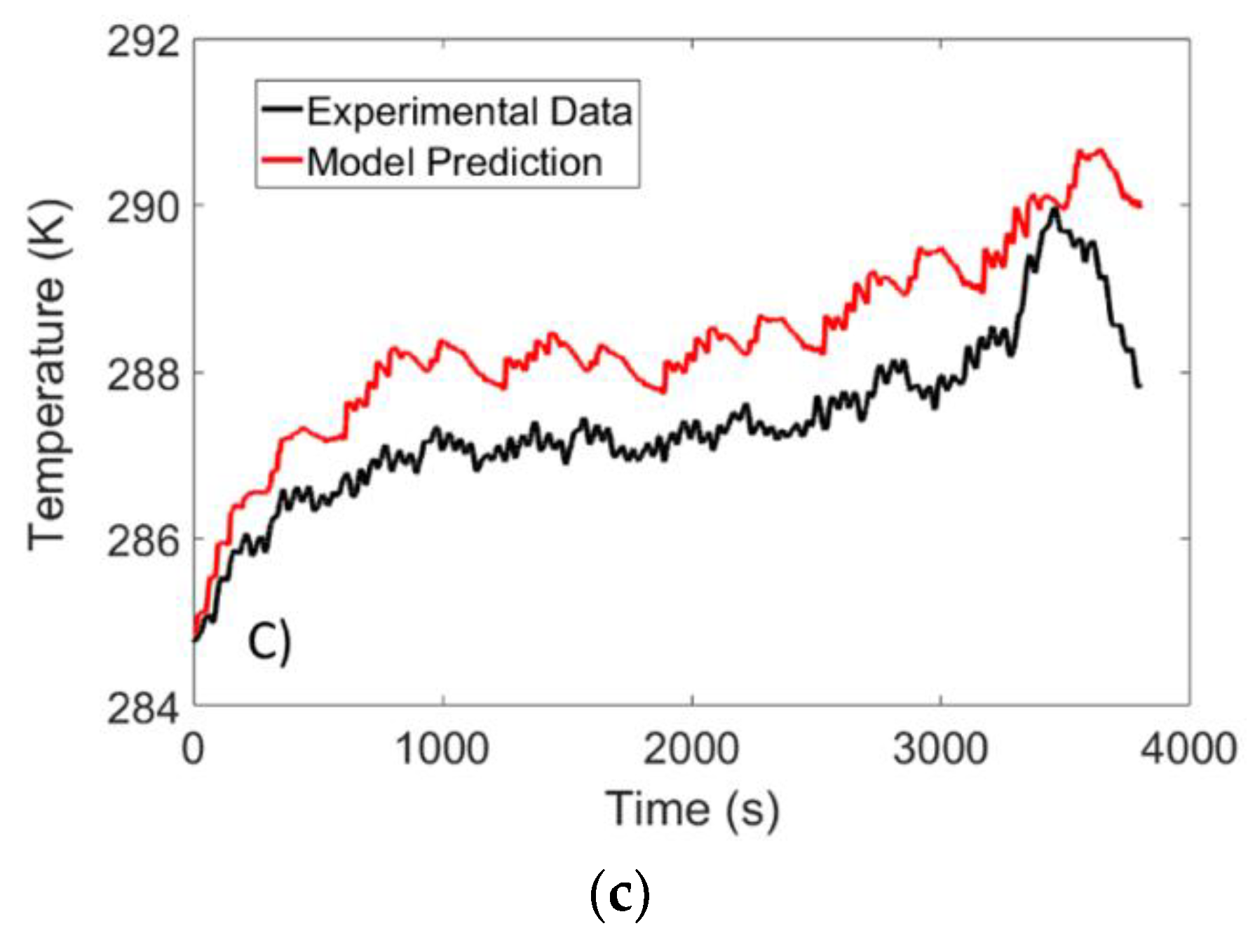
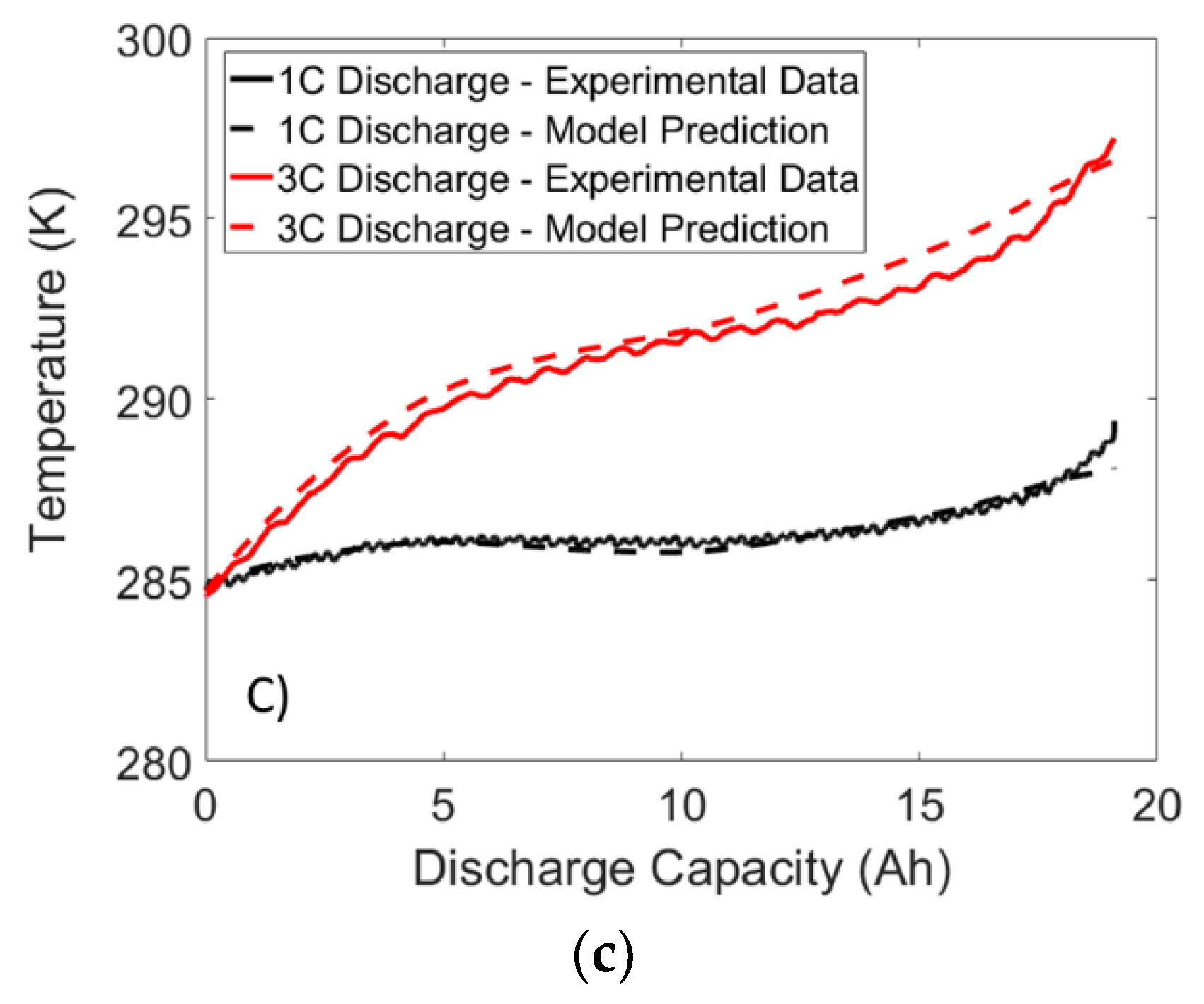
4.3. Temperature Validation Results

Once the ECM parameter sub-model was developed, it was incorporated into the overall battery modeling framework to estimate the temperature and voltage response. To validate the temperature, the Li-Ion battery was charged to full and brought to empty using the US-06 drive cycle. The US-06 drive cycle is used to simulate aggressive highway and city driving and can be converted to a current profile using Autonomie software. A Malibu plug-in hybrid, with a 19.7 kWh battery pack consisting of seven 15s3p modules, was used to generate the profile. Although the battery pack was sized for AMP20 pouch batteries, it can be scaled to any size. The current profile for one US-06 cycle is shown in Figure 11.

The validation test was carried out at ambient temperatures of 10 °C, 25 °C and 40 °C and the temperature was monitored using the set-up described in Section 2. The temperature predicted by the model was compared to that obtained from the validation experiment, and the results are illustrated in Figure 12.

Figure 12 shows good agreement between the predicted temperature and the experimental data for experiments carried out at 25 °C and 40 °C. To report the error quantitatively, the root mean squared error (RMSE) can be calculated. The equation for calculating the RMSE for N samples is shown below.

$$RMSE=\sqrt{\frac{{{\displaystyle \sum }}_{i=1}^N{\left(Y_{pred,i}-Y_{exp,i}\right)}^2}{N}}$$

(15)

where Y_i,pred and Y_i,exp are used to represent the predicted and experimental voltage or temperature. The RMSE value reported in this work will be calculated between the 90% and 10% SOC interval since the models were identified for this particular region.

For the experiments carried out at 25 °C and 40 °C, the RMSE was determined to be 0.32 K and 0.18 K, respectively. The largest deviation between experimental data and model data was detected at 10 °C, where an RMSE value of 1 °C was observed. Although the error is higher for low temperatures, the accuracy of the model is similar to predictive models that have been proposed in the literature [17,29]. Finally, it should be noted that the sudden drop in temperature at the end of the test is due to the entropic heat generation term that resembles an endothermic process at low SOC values.

In addition to a drive cycle, the predictive capability of the comprehensive model was further validated by conducting a constant current 1C and 3C discharge experiment. Before discharging, the battery was allowed to rest for 1 h to ensure it reached thermal equilibrium. The results are summarized in Figure 13.

When examining Figure 12 and Figure 13, it is apparent that the temperature response dips slightly at the mid SOC region. This dip is a result of the positive dU_ocv/dT values observed in Figure 13 at the middle SOC region, resulting in a lower heat generation and thus a smaller temperature rise. Therefore, the results demonstrate the importance of using the reversible heat generation term when exact prediction of temperature is required. In addition, strong agreement is found between model and experiment at all temperatures and C-rates. Therefore, the results from these validation experiments suggest that the proposed framework can be utilized by future researchers to accurately predict the temperature response of the battery under dynamic load.

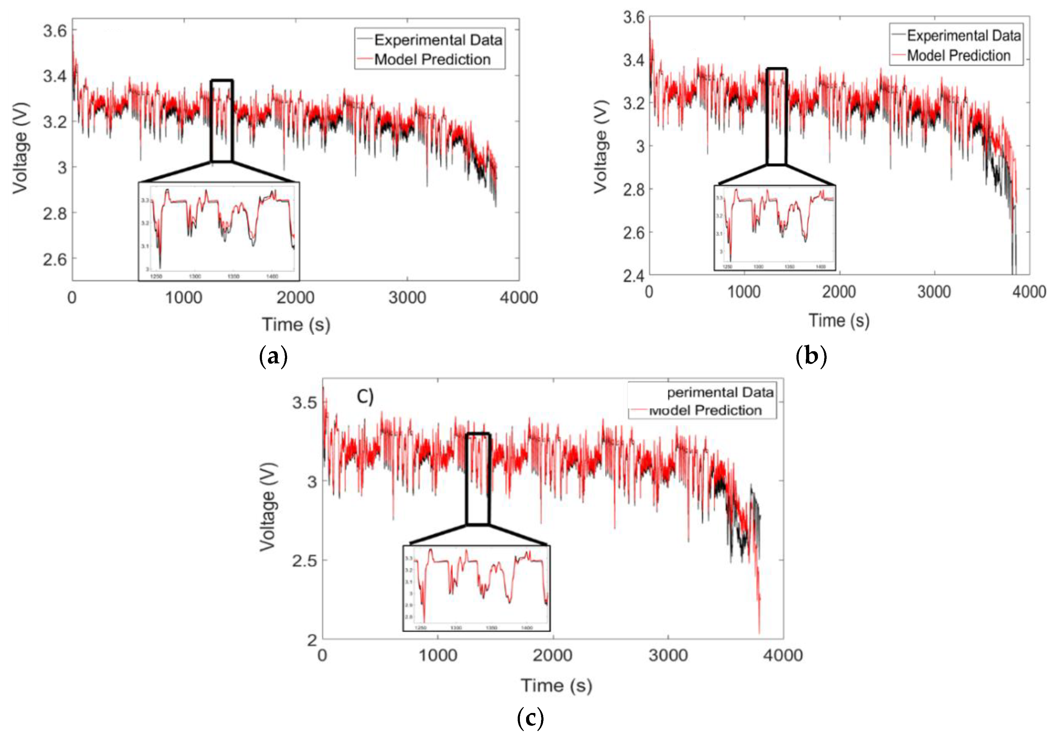
4.4. Voltage Validation Results

A comprehensive battery simulator should not only be able to predict the cell temperature but also accurately capture the voltage drops across the battery terminal. The voltage profiles for the US-06 drive cycle and the 1C/3C discharge cycle are shown in Figure 14 and Figure 15, respectively.

Inspection of the discharge curves (Figure 15) indicates strong agreement between the model and experimental data for most voltage profiles. Within the 90% to 10% SOC range, the maximum RMSE value was determined to be 38 mV, which is similar to the values obtained by Lin et al. [17]. The model does deviate from the experimental data, however, towards the end of the cycle. One possible reason for this discrepancy could be that the capacity of the battery is not being modeled as a function of temperature. The drive cycle profiles reveal a similar trend, where the model deviates from experimental data at 10 °C. Future work can be carried out to determine whether this effect at cold temperatures can be incorporated by using additional RC pairs that are dependent on the battery temperature.

4.5. Comparison to Existing Approaches

The results reported in Section 4.3 and Section 4.4 show that the proposed model can sufficiently capture the temperature and voltage response of an LFP battery under dynamic loads. By using a DOE approach, an accurate battery model can be developed without the need to run an inordinate number of experiments. However, it is important to understand how accurate the ECM parameter surface is in comparison to existing techniques. Therefore, additional experiments were carried out at temperatures from 5 °C to 45 °C in intervals of 10 °C and from 90% to 10% SOC in intervals of 10%.

As previously mentioned, there are two techniques that are frequently used to model the ECM parameter response surface. The first method uses a look-up table (LUT), where sample points in-between are determined through linear interpolation. The second approach, referred to in this work as Non-DOE approach, uses all the data points to develop an empirical model. The approach proposed in this work uses a total of 14 runs, whereas the two commonly used techniques require 50 runs in total. Assuming each experiment takes 2 h to conduct, this translates to reducing the characterization time from 100 h to just 28 h.

Using the additional 50 experiments, a LUT model and Non-DOE empirical model were developed and added to the existing battery simulation framework. The same validation profiles shown in Section 4.3 and Section 4.4 were run through the simulator and the root mean squared error for both temperature and voltage were determined. The RMSE for the temperature response from the battery simulator is shown in

Table 6. Root mean squared error for the temperature response for LUT and Non-DOE techniques in comparison to the face-center CCD approach.

Temperature RMSE (K)
Type	10 °C			25 °C			40 °C
	LUT	Non-DOE	CCD	LUT	Non-DOE	CCD	LUT	Non-DOE	CCD
1C Discharge	0.17	0.17	0.18	0.17	0.17	0.19	0.34	0.40	0.44
3C Discharge	0.60	0.65	0.57	0.59	0.35	0.26	0.47	0.33	0.25
us 06	0.95	1.07	1.07	0.37	0.32	0.25	0.31	0.18	0.13
Average	0.57	0.63	0.61	0.38	0.28	0.23	0.37	0.30	0.27

.

First, examining the temperature errors from the proposed approach (CCD), the highest error is observed for the US-06 drive cycle at a temperature of 10 °C. This error value is consistent with electro-thermal models proposed by Damay et al. [19], Lin et al. [17] and Sun et al. [30], where maximum RMSE values around 1 K were observed. Therefore, the results from this table further confirm the fact that the electro-thermal model can adequately predict the temperature rise in the battery. This is true for both drive cycles as well as constant current discharges.

Next, it should be noted that similar RMSE values are observed in all three approaches. In some situations, the CCD design fares better, and, in others, it fares worse. Therefore, by using the CCD technique, the same degree of accuracy can be obtained while significantly reducing the time required to identify the model. The same analysis can be carried out for the voltage response of the battery and the results are summarized in

Table 7. Root mean squared error for the temperature response for LUT and Non-DOE techniques in comparison to the face-center CCD approach.

Voltage RMSE (mV)
Type	10 °C			25 °C			40 °C
	LUT	Non-DOE	CCD	LUT	Non-DOE	CCD	LUT	Non-DOE	CCD
1C Discharge	35.7	31.9	29.3	9.1	10.3	11.5	30.0	35.1	38.5
3C Discharge	45.0	47.1	40.9	38.9	29.6	21.2	15.8	9.3	15.8
US-06	26.7	22.2	20.8	19.5	22.6	24.7	13.0	18.1	22.4
Average	35.8	33.7	30.3	22.5	20.8	19.1	19.6	20.8	25.6

.

The highest voltage RMSE errors, observed for 3C discharge, are similar in values to those obtained by Lin et al. [17], where the maximum RMSE value was found to be 45 mV. In addition, no difference is observed between the three approaches, leading to the conclusion that additional experiments will not yield more accurate results.

5. Conclusions

This work developed a compressive battery simulator for predicting the voltage and temperature response of an LFP battery under load. An ECM was used for modeling the battery voltage change while a thermal and heat generation model was developed for describing the temperature change. A DOE approach was used for generating the ECM parameter response surface.

The main conclusions from this works are as follows:

• The model developed in this paper can accurately predict the temperature and voltage profiles of an LFP battery.
• All three ECM parameters were highly dependent on temperature and SOC, although only a linear dependence was observed for the Thevenin resistance.
• Replication runs are essential for accurately quantifying measurement noise and identifying which parameters in the model are significant. Conducting a statistical analysis is important as it allows one to draw conclusions on which factors affect the ECM parameters. This knowledge can be useful when developing robust state estimators that require determining the ECM parameters in real time.
• Using a DOE approach, the same degree of accuracy as existing techniques can be achieved while reducing the characterization time from 100 h to just 28 h. This time reduction is even more substantial if an additional SOH variable is added. Therefore, the DOE approach proposed in this paper provides a framework that future researchers can use to develop a comprehensive battery model that includes battery degradation.

References

1. Tarascon, J.; Armand, M. Issues and challenges facing rechargeable lithium batteries. Nature 2001, 414, 359–367. [Google Scholar] [CrossRef] [PubMed]
2. Huat, L.; Ye, Y.; Tay, A.A.O. Integration issues of lithium-ion battery into electric vehicles battery pack. J. Clean. Prod. 2016, 113, 1032–1045. [Google Scholar]
3. Manzetti, S.; Mariasiu, F. Electric vehicle battery technologies: From present state to future systems. Renew. Sustain. Energy Rev. 2015, 51, 1004–1012. [Google Scholar] [CrossRef]
4. Santhanagopalan, S.; Guo, Q.; Ramadass, P.; White, R.E. Review of models for predicting the cycling performance of lithium ion batteries. J. Power Sources 2006, 156, 620–628. [Google Scholar] [CrossRef]
5. Farkhondeh, M.; Delacourt, C. Mathematical Modeling of Commercial LiFePO4 Electrodes Based on Variable Solid-State Diffusivity. J. Electrochem. Soc. 2012, 159, A177–A192. [Google Scholar] [CrossRef]
6. Mastali, M.; Farhad, S.; Farkhondeh, M.; Fraser, R.A.; Fowler, M. Simplified electrochemical multi-particle model for LiFePO4cathodes in lithium-ion batteries. J. Power Sources 2015, 275, 633–643. [Google Scholar] [CrossRef]
7. Mastali, M.; Kohneh, M.; Samadani, E.; Fraser, R.; Fowler, M. Three-Dimensional Electrochemical Analysis of a Graphite/LiFePO4 Li-Ion Cell to Improve Its Durability; SAE Technical Paper; SAE: Detroit, MI, USA, 2015. [Google Scholar]
8. Mastali, M.; Samadani, E.; Farhad, S.; Fraser, R.; Fowler, M. Three-dimensional Multi-Particle Electrochemical Model of LiFePO4 Cells based on a Resistor Network Methodology. Electrochim. Acta 2016, 190, 574–587. [Google Scholar] [CrossRef]
9. Mastali, M.; Farkhondeh, M.; Farhad, S.; Fraser, R.A.; Fowler, M. Electrochemical Modeling of Commercial LiFePO4 and Graphite Electrodes : Kinetic and Transport Properties and Their Temperature Dependence. J. Electrochem. Soc. 2016, 163, A2803–A2816. [Google Scholar] [CrossRef]
10. Panchal, S.; Mathew, M.; Fraser, R.; Fowler, M. Electrochemical thermal modeling and experimental measurements of 18650 cylindrical lithium-ion battery during discharge cycle for an EV. Appl. Therm. Eng. 2018, 135, 123–132. [Google Scholar] [CrossRef]
11. Seaman, A.; Dao, T.-S.; McPhee, J. A survey of mathematics-based equivalent-circuit and electrochemical battery models for hybrid and electric vehicle simulation. J. Power Sources 2014, 256, 410–423. [Google Scholar] [CrossRef] [Green Version]
12. Samadani, E.; Farhad, S.; Scott, W.; Mastali, M.; Gimenez, L.E.; Fowler, M.; Fraser, R.A. Empirical Modeling of Lithium-ion Batteries Based on Electrochemical Impedance Spectroscopy Tests. Electrochim. Acta 2015, 160, 169–177. [Google Scholar] [CrossRef]
13. Mathew, M.; Kong, Q.H.; McGrory, J.; Fowler, M. Simulation of lithium ion battery replacement in a battery pack for application in electric vehicles. J. Power Sources 2017, 349, 94–104. [Google Scholar] [CrossRef]
14. Murashko, K.; Pyrhonen, J.; Laurila, L. Three-dimensional thermal model of a lithium ion battery for hybrid mobile working machines: Determination of the model parameters in a pouch cell. IEEE Trans. Energy Convers. 2013, 28, 335–343. [Google Scholar] [CrossRef]
15. Samadani, E.; Mastali, M.; Farhad, S.; Fraser, R.A.; Fowler, M. Li-ion battery performance and degradation in electric vehicles under different usage scenarios. Int. J. Energy Res. 2015, 40, 379–392. [Google Scholar] [CrossRef]
16. Hu, Y.; Yurkovich, S.; Guezennec, Y.; Yurkovich, B.J. Electro-thermal battery model identification for automotive applications. J. Power Sources 2010, 196, 449–457. [Google Scholar] [CrossRef]
17. Lin, X.; Perez, H.E.; Mohan, S.; Siegel, J.B.; Stefanopoulou, A.G.; Ding, Y.; Castanier, M.P. A lumped-parameter electro-thermal model for cylindrical batteries. J. Power Sources 2014, 257, 1–11. [Google Scholar] [CrossRef]
18. Samadani, E.; Gimenez, L.; Scott, W.; Farhad, S.; Fowler, M.; Fraser, R. Thermal Behavior of Two Commercial Li-Ion Batteries for Plug-in Hybrid Electric Vehicles; SAE Technical Paper; SAE: Detroit, MI, USA, 2014. [Google Scholar]
19. Damay, N.; Forgez, C.; Bichat, M.P.; Friedrich, G. Thermal modeling of large prismatic LiFePO4/graphite battery. Coupled thermal and heat generation models for characterization and simulation. J. Power Sources 2015, 283, 37–45. [Google Scholar] [CrossRef]
20. Jaguemont, J.; Boulon, L.; Dube, Y. Characterization and Modeling of a Hybrid-Electric-Vehicle Lithium-Ion Battery Pack at Low Temperatures. IEEE Trans. Veh. Technol. 2016, 65, 1–14. [Google Scholar] [CrossRef]
21. Mastali, M.; Foreman, E.; Modjtahedi, A.; Samadani, E.; Amirfazli, A.; Farhad, S.; Fraser, R.A.; Fowler, M. Electrochemical-thermal modeling and experimental validation of commercial graphite/LiFePO4 pouch lithium-ion batteries. Int. J. Therm. Sci. 2018, 129, 218–230. [Google Scholar] [CrossRef]
22. Montgomery, D. Design and Analysis of Experiments, 8th ed.; John Wiley & Sons, Inc.: Hoboken, NJ, USA, 2013. [Google Scholar]
23. Khuri, A.; Mukhopadhyay, S. Response surface methodology. Comput. Stat. 2010, 2, 128–149. [Google Scholar] [CrossRef] [Green Version]
24. Vera, L.; De Zan, M.M.; Cámara, M.S.; Goicoechea, C. Talanta Experimental design and multiple response optimization. Using the desirability function in analytical methods development. Talanta 2014, 124, 123–138. [Google Scholar] [CrossRef] [PubMed]
25. Rao, L.; Newman, J. Heat-Generation Rate and General Energy Balance for Insertion Battery Systems. Electrochem. Soc. 1997, 144, 2697–2704. [Google Scholar] [CrossRef]
26. Mastali, M. Electrochemical-Thermal Modeling of Lithium-ion Batteries. Ph.D. Thesis, University of Waterloo, Waterloo, ON, Canada, 2016. [Google Scholar]
27. Bandhauer, T.M.; Garimella, S.; Fuller, T.F. A Critical Review of Thermal Issues in Lithium-Ion Batteries. J. Electrochem. Soc. 2011, 158, R1–R25. [Google Scholar] [CrossRef]
28. Jalkanen, K.; Aho, T.; Vuorilehto, K. Entropy change effects on the thermal behavior of a LiFePO4/graphite lithium-ion cell at different states of charge. J. Power Sources 2013, 243, 354–360. [Google Scholar] [CrossRef]
29. Farag, M.; Sweity, H.; Fleckenstein, M.; Habibi, S. Combined electrochemical, heat generation, and thermal model for large prismatic lithium-ion batteries in real-time applications. J. Power Sources 2017, 360, 618–633. [Google Scholar] [CrossRef]
30. Sun, J.; Wei, G.; Pei, L.; Lu, R.; Song, K.; Wu, C.; Zhu, C. Online internal temperature estimation for lithium-ion batteries based on Kalman filter. Energies 2015, 8, 4400–4415. [Google Scholar] [CrossRef]
Figure 1. Experimental set-up for model development and voltage validation.
Batteries 04 00029 g001
Figure 2. The experimental set-up of the LFP cell: (a) Picture of the cell inside the thermal chamber; (b) Schematic of the thermocouple placements on the LFP cell.
Batteries 04 00029 g002
Figure 3. The temperature profile used for determining dUocv/dT term.
Batteries 04 00029 g003
Figure 4. Overall comprehensive battery simulator with all four sub-models.
Batteries 04 00029 g004
Figure 5. ECM with an open circuit voltage source, an ohmic resistance with n RC pairs in series.
Batteries 04 00029 g005
Figure 6. Face-centered CCD for ECM parameter surface.
Batteries 04 00029 g006
Figure 7. The open circuit voltage obtained by averaging the C/25 charge and discharge curves.
Batteries 04 00029 g007
Figure 8. The experimentally determined values of dUocv/dTc as a function of SOC.
Batteries 04 00029 g008
Figure 9. The experimental and fitted values for the cooling curves at 1C, 2C and 3C discharge.
Batteries 04 00029 g009
Figure 10. Response surface plots and experimental data for: (a) ohmic resistance; (b) Thevenin resistance; and (c) Thevenin capacitance parameters.
Batteries 04 00029 g010
Figure 11. Current profile for a US-06 drive cycle simulated in Autonomie.
Batteries 04 00029 g011
Figure 12. Temperature response of a LFP battery subject to a US-06 drive cycle at ambient temperatures of: (a) 40 °C; (b) 25 °C; and (c) 10 °C.
Batteries 04 00029 g012aBatteries 04 00029 g012b
Figure 13. Temperature response of a LFP battery subjected to constant current 1C and 3C discharge at ambient temperatures of: (a) 40 °C; (b) 25 °C; and (c) 10 °C.
Batteries 04 00029 g013aBatteries 04 00029 g013b
Figure 14. The predicted and simulated voltage profile at 1C and 2C/3C charge for temperatures of: (a) 10 °C; (b) 25 °C; and (c) 40 °C.
Batteries 04 00029 g014
Figure 15. The predicted and simulated voltage profile at 1C and 2C/3C discharge for temperatures of: (a) 10 °C; (b) 25 °C; and (c) 40 °C.
Batteries 04 00029 g015