Comparison of Battery Architecture Dependability


Univ Lyon, Université Claude Bernard Lyon 1, École Centrale de Lyon, INSA Lyon, CNRS, Ampère, F-69622 Villeurbanne, France
*
Author to whom correspondence should be addressed.
Batteries 2018, 4(3), 31; https://doi.org/10.3390/batteries4030031
Submission received: 14 May 2018
/
Revised: 7 June 2018
/
Accepted: 7 June 2018
/
Published: 3 July 2018
(This article belongs to the Special Issue Batteries and Supercapacitors Aging)
Abstract
:This paper presents various solutions for organizing an accumulator battery. It examines three different architectures: series-parallel, parallel-series and C3C architecture, which spread the cell output current flux to three other cells. Alternatively, to improve a several cell system reliability, it is possible to insert more cells than necessary and soliciting them less. Classical RAMS (Reliability, Availability, Maintainability, Safety) solutions can be deployed by adding redundant cells or by tolerating some cell failures. With more cells than necessary, it is also possible to choose active cells by a selection algorithm and place the others at rest. Each variant is simulated for the three architectures in order to determine the impact on battery-operative dependability, that is to say the duration of how long the battery complies specifications. To justify that the conventional RAMS solutions are not deployed to date, this article examines the influence on operative dependability. If the conventional variants allow to extend the moment before the battery stops to be operational, using an algorithm with a suitable optimization criterion further extend the battery mission time.
1. Context
An electrical energy storage systems (EESS) may be an electrochemical cell association in a battery [1]. These cells can belong to different technologies and chemistries. The oldest are lead–acid cells. Then, there are the cells using alkaline metals. Finally, for a quarter of a century, lithium cells have been marketed. Lithium-ion cells are more stable than the first lithium cells and have higher energy and power densities than the lead–acid and nickel-based technologies [2]. They also have a higher lifespan, which partly explains their strong growth. The lithium-ion battery market continues to grow, to the point that their unit manufacturing price decreases steadily because of the growing number of units produced [3]. Naturally, in a battery, all cells belong to the same technology.
This paper presents three architectures that can be used in cell batteries: two classics, using permanent series and parallel connections between cells, and one innovative, described later and allowing different connections between the cells. On these architectures, different variants are tested: common solutions (balancing between cells, using of more cells than necessary to provide the nominal power), other conventional but not deployed in best industrial solutions (failure tolerance of some cells with over-solicitation of others, addition of redundant cells to replace the first failing cells) and a new variant (redundant cells management with a control law using cells fundamental states as a choice criterion). The performances of the architectures and their variants are compared by simulation under Matlab, by resorting to a cell model that including aging phenomena.
The cell main electrical characteristic is its maximum storable capacity Q0. It is well known that this capacity decrease with aging. When a cell is new, this capacity is optimal. It is noted in this paper as Q*. The battery physical behavior can be modeled by a second order Thevenin model scheme [4] as seen in Figure 1. In this, a cell is represented as a series association of an open-circuit voltage (OCV), an equivalent series resistance (ESR) and a parallel RC circuit. The ESR corresponds to the battery terminals voltage Vcell, only if it is measured without an external load connection and with the cell at rest for an adequate time. This time is necessary for balancing internal electrical charges (relaxation phenomenon). A double-layer capacitance (Cw) and a charge transfer resistance (Rw) complete the model by describing relaxation. Other internal phenomena such as a hysteresis voltage can also be modeled by additional subcircuits. Hysteresis consists in a shifting on the open-circuit voltage for the same contained charge between current direction, an upward offset with a negative current Icell in charging phase and a downset offset with a positive current in the discharge phase.
To express physical state in which a cell is, two indicators are commonly used: SoC and SoH, respectively, the state of charge and the state of health [5]. The SoC describes, in percent, the amount of electrical charge Q(t) it contains at t time, compared to its maximum storable capacity. The SoC is determined by Equation (1). Moreover, when a cell ages, it cannot store as much electrical charge than when it is new. The maximum storable capacity Q0 decreases over time continuously and gradually from its optimal capacity Q*. So, a cell’s State of Health (SoH) is defined by the ratio between these two capacity values, as shown by Equation (2). For applications requiring significant power more than a willingness to deliver energy, SoH can also be defined relative to the ESR [6].
The ISO 12405-2 standard for electric vehicles [7] specifies test procedures for lithium-ion batteries and electrically propelled road vehicles. It specifies that a cell enters the old age phase when its SoH goes down to 80%. Manufacturers communicate a lifetime value for cells that incorporate, as specified in their datasheet, the two aging modes that a cell faces: an age-related calendar mode [8] and a cyclic mode related to cell use [9]. These two phenomena [10] can be described by a combined evolution of a linear aging and an “aging” power of time whose principles are described by Equation (3), where the aging parameter is between 0.5 and 2 and A1 and A2 are two constants.
Cyclic aging is aggravated mainly by three parameters: the operating temperature [11], the amount of electrical charge extracted in a cycle [12] and the current [13]. Despite the cell manufacturing standardization, disparities can occur between cells from the same batch. These are reflected in an optimal capacity Q* variability and in an equivalent series resistances ESR variability [14]. Thus, when cells are associated in an EESS, their disparities should lead to imbalances in currents, cell temperatures and then in their aging. Consequently, a battery may remain operational for a shorter time than a cell lifetime.
Operative dependability Odep is defined as the time, expressed in hours or in number of cycles, during which a multi-cellular battery can meet the external load specifications [15]. In other words, Odep is the time before a downtime related to a full discharge or a too high age. That is to say, it contains enough operational cells to provide the requested power. For a single cell, this cessation comes from:
- −
- a cell aging failure, resulting in a SoH of less than 0.8;
- −
- a sudden random failure (open or short circuit);
- −
- a complete discharge, SoC drops down to zero in operating phase.
For a battery, Odep depends on the architecture (how cells are connected); if some cells are in redundancy for the current mission and if failed cells can be isolated or not. It is therefore necessary to monitor the cell states. In order to monitor cells, in particular to control end of charging and to prevent overheating, EESS cells are managed by a BMS (Battery Management System) [16]. Today, multi-cellular EESS are constituted according to two conventional architectures (series-parallel and parallel-series) and sometimes include variants, as explained in the next section, to improve their availability.
From a formal point of view, the operative dependability Odep is defined by the equation set (4), according to SoC and SoH cells.
In the next section, different architectures and possible variants to improve the battery operative dependability are presented. Then, part III presents simulations performed on each variant, whatever the cell technology, in order to determine the impact on operative dependability, for LiFePO4 cell example. The next part presents and compares the simulation results, especially for operative dependability.
2. Architectures and Variants
In the literature, to improve the operative dependability, various solutions for reconfiguration of the internal structure are proposed, such as the power tree solution presented in [17] or the DESA architecture (Dependable, efficient, scalable architecture) [18]. The first solution does not allow use of a battery at full power and the second only improves the operative dependability of a similar order to the amount of additional cell number (typically 50% with 50% of additional cells).
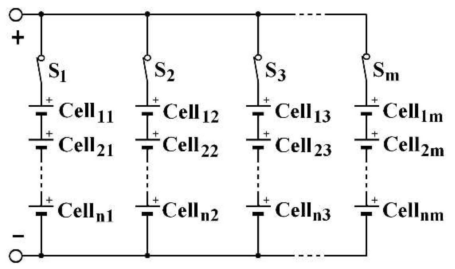
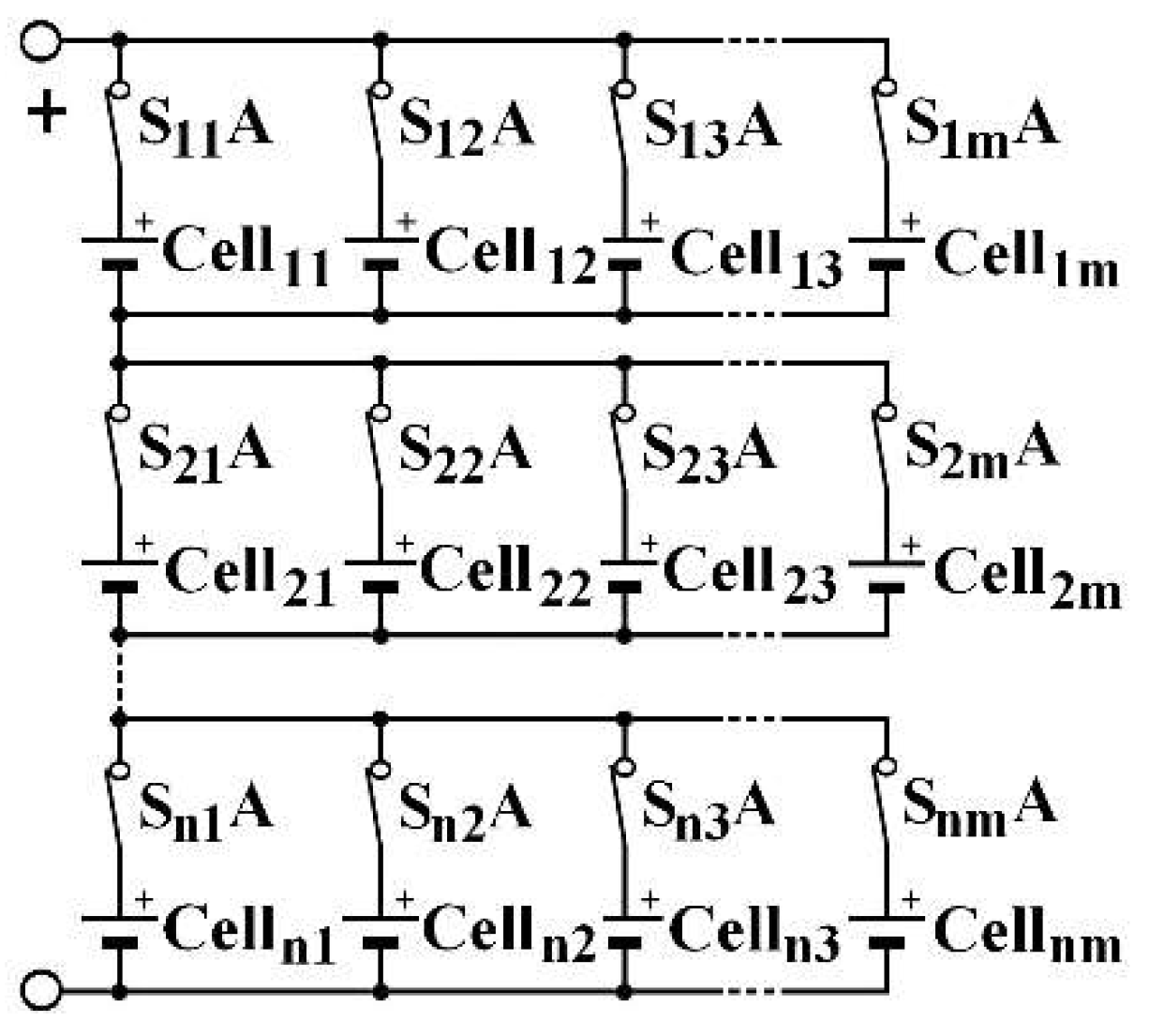
Three architectures are compared to determine which has the best operative dependability: two conventionally used and a new one. These architectures are reconfigurables by using a limited number of switches associated with a cell. To increase the battery voltage, the cells are associated in series. To increase the current, they are associated in parallel. Thus, batteries are generally associated in a SP (series-parallel) architecture, as described in Figure 2, which presents a n-rows m-columns structure, noted (n, m). Switches allow to isolate a column, following one of its cell failure, for instance. By duality, the same structure can be inserted into a PS (parallel-series) architecture, as shown in Figure 3. One switch for each cell is needed in order to isolate a failed cell. In an SP architecture, same-column cell voltage disparities can appear. In a PS architecture, the same-row cell currents can be different.
To deliver the same power, by keeping the same structure, another architecture is possible: the C3C [19], depicted in Figure 4. The architecture consists of an element association. Each C3C element comprises a cell and three switches, as shown by Figure 5. Each includes an upstream connection and three downstream. The A indexed switch is placed on the upstream connection. Switch B is on the first downstream connection, C on the third. The middle connection is intended to be connected with the same-column downstream-row cell upstream connection. The C3C architecture combines the advantages of both conventional architectures, as PS’ self-balancing and allows a series association of some cells located on different columns. The current that leaves the Celli,j in the ith row and the jth column can be directed to one of the three following row cells: Celli+1,j−1, Celli+1,j, Celli+1,j+1, in a recharge phase, respectively by the switches Si,jB, Si+1,jA and Si,jC or to one of the three upstream row cells: Celli−1,j−1, Celli−1,j, Celli−1,j+1, in a discharge phase. This is made by activating the appropriate switches, respectively Si−1,j−1C, Si,jA and Si−1,j+1B. Thanks to the architecture, the mth column cells are connected with those of the first column.
The C3C architecture involves two particularities. Firstly, to take advantage of its very large possible configuration number [20], it must be managed by an algorithm that chooses the best cell combination, with a cell-aging-reducing aim. The cells selection parameters can be chosen to define the optimal combination. Only two are considered in this paper: SoC and SoH. Secondly, whatever the architecture, to increase battery reliability, a minimum amount of redundancy must be included [21]. This minimal part consists of using a column (especially the mth) as a redundant column. Thus, a (n, m) battery is calibrated to provide a nominal power Pn given by Equation (5).
As a result, if the conventional architectures include a redundant column, they can also be managed by the same algorithm that chooses the best cell combination. The possible combination number is nevertheless much lower. Therefore, if the battery must supply its nominal current Inom, depict in Equation (6), one cell in each row stays at rest. In PS and C3C architectures, this cell can be any of the m cells of each row. In SP, all the same-column cells are placed at rest. To do this, it requires adding a switch in series with each cell in PS and one by column in SP, as shown in Figure 2 and Figure 3.
If SP and PS batteries include a redundant column, it becomes possible to use this redundancy classically. That is, the battery can work with its base cells, corresponding to the first (m−1) columns, until one of them stops to be operational. It is thus replaced by the spare cell. In this variant, the mth switches in the Figure 3 are off in the beginning for a PS architecture. For an SP architecture, in Figure 2, all cells in the mth column are redundant.
Another variant can also be examined, tolerating a cell failure by replacing it with a short circuit in SP architecture and allowing the battery to continue to fulfill its mission, even if it requires the active cells to afford a greater current than their nominal current. To do so, two switches should be placed around each cell: one in series and one in parallel as Si,jA is being open and Si,jB closed when celli,j must be isolated, as depicted for cell22, as shown by Figure 6. In this example, cell22 fails, the current of the second column passes through S22B. The cell is marked with a red cross to symbolize its failure. This variant does not require redundancy cells. The same power as in Equation (5) is obtained with a (n, m−1) structure. In a PS architecture, the cell may just be disconnected by only one switch, as shown for cell22 in Figure 7, in which cell1m−1 and cell22 are faulty and marked with a red cross.
It is also possible to use a battery comprising m columns to provide a power corresponding to the nominal power of Equation (5). In this way, the battery has an over-capacity compared to the external load specifications.
Moreover, in order to reduce the disparities between the SoCs when cells are associated in series, in an SP architecture, balancing circuits are often used. They enable to homogenize the electrical charges in all cells in the string [22]. These balancing circuits are controlled by a BMS [23]. They allow better stored energy use [24] and a battery operative dependability improvement [25,26]. To evaluate balancing impact, basic SP of Figure 2 (with (m−1) columns) with and without balancing circuits are simulated. All compared batteries must provide the same Equation (5) power. So, this structure only includes (m−1) columns. Several balancing techniques exist in an SP architecture:
- −
- dissipative balancing [27], consisting of balancing the electrical charges from below by removing excess energy by Joule effect;
- −
- redistributive balancing to send excess energy from the most charging cell(s) to the least charging cell(s) in the same column [28]. Its principle is described by the Figure 8 scheme, relating to a single column j in an SP architecture. When Cella,j is more charged than Cellb,j, the intermediate capacitor Cbj, associate to this column j, is placed in parallel by switching on the Sa,j+ and Sa,j− switches. Then, these switches are switched off and the Sb,j+ and Sb,j− switches are switched on. At the end, Cellaj electric charge have been reduced and Cellaj one have been increased.
In this study, only redistributive balancing circuits from one cell to another are considered. This leads to add two switches by cell in SP schemes, each connecting a terminal of the cell to a terminal of an intermediate capacitor, used to temporarily store the energy to be transferred. By this way, the different variants combining architecture and improvement are listed in Table 1. The structure column number mc and the cell-associated switch number are also specified. For the basic PS and the over-capacity PS variants, the switches in Figure 3 are not useful because cells are not managed individually. The cells are all active or all inactive. In the same way, those of Figure 2 are not useful in the without-balancing SP variant. Apart from the variant reported without balancing, all other SPs include balancing circuits, which add two switches per cell. The variants deployed in present industrial solutions are PS-base, SP-base with or without balancing and over-capacity variants.
3. Simulations
The different variants and architectures were modeled using Matlab. The program simulates cell associations according to each architecture for different (n, m) structures. For each variant, it submits the battery to regular cycling, leading the current shown in Figure 9 for a single 10 Ah cell. The battery is initially full. This cycle consists of firstly, a discharge under a current I equal to the battery nominal current Inom divided by the active column number mc (that is to say (m−1) or m) for a duration of 2500 s. So, except for over-capacity variants, I = 10 A in discharging phase. By this way, the battery is discharged by 70% of its initial capacity. This discharge value is relevant for quantifying cell aging. Indeed, it allows to stop the discharging phase before a complete discharge. The more Qo(t) decreases, the more the SoC at the end of discharging phase decreases. This is because a cell has to provide the same amount of energy. Then, the cells are recharged, for the same duration, to return to full charge. Finally, the battery is placed at rest for an identical duration, allowing the return to internal balance.
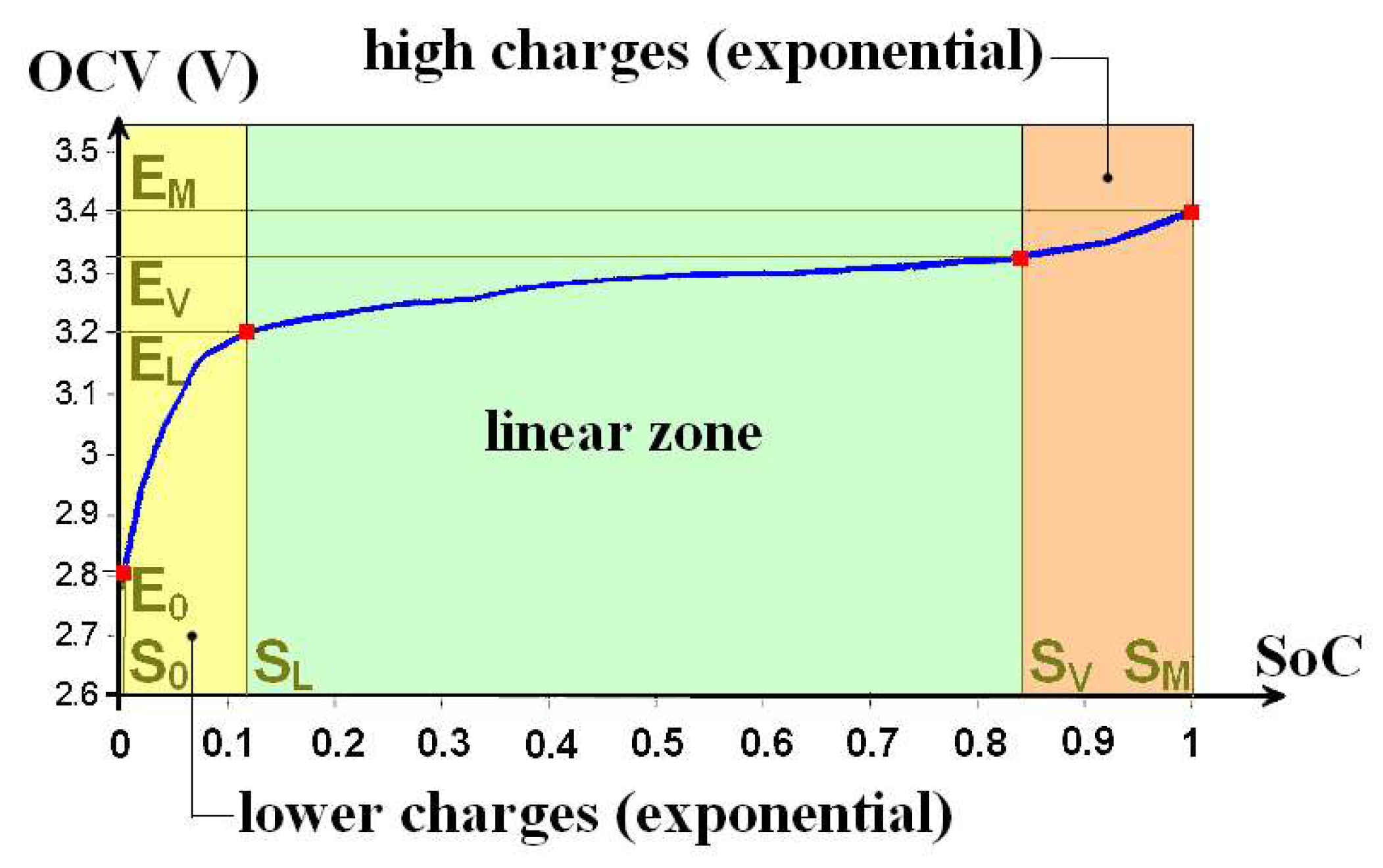
To model a cell, a characteristic equation that describes the OCV evolution as a function of the SoC is used. The typical shape of this curve is described for an amorphous iron phosphate (LiFePO4) cell in Figure 10. Batteries, with an amorphous iron phosphate positive electrode support high intensities in charge and discharge as well as fast charges. These cells have higher power density and lower fire risks than cells with a lithium cobalt oxide (LiCoO2) positive electrode [29]. On this curve, four points are identified by a red dot. These four coordinate points (S0, E0), (SL, EL), (SV, EV) and (SM, EM), respectively, delimit three sectors. The curve being continuous, it is so possible to perform partial regression. In the sector where the state of charge is low (SoC < SL) and OCV low (OCV < EL), the curve can be described by an exponential function. It is the same for high states of charge (SoC > SV and OCV > EV). The central sector can be described by a linear function. Ultimately, the characteristic equation can be described by equation set (7) as a function of the SoC (explain as a dummy variable x). ν and ξ parameters are empirical. ν is between 10 and 20. It corresponds to the rapid growth of the voltage when the SoC approaches its maximum. ξ parameter is its complement when the voltage collapses, the SoC decreasing towards its minimum.
In these simulations, the cells had an initial capacity Q* = 10 Ah and an average ESR of 20 mΩ. The ambient temperature was set to 25 °C. Since the Q0(t) degradation is continuous and progressive, it is logical to consider that the SoH, which is a representation of this degradation, also decreases continuously. This degradation is proportional to the using conditions. At each cycle, a cell ages. This translates into an SoH decrease.
The cell temperature evolves as a function of the current flowing through it. By convection, radiation and conduction, this heat can spread to other cells. For simplicity, the used model does not integrate thermal coupling phenomena.
Finally, the initial conditions for each cell was given randomly around nominal a value with a variability of more or less 10%. The same Celli,j is used for all variants in all architectures, so as to ensure a true comparison of the variant intrinsic performance. A cell is considered faulty in two cases. First, when it is completely discharged whereas it should still supply energy (SoC = 0). Second, when it is too old and has SoH = 0.8. This corresponds, for a single cell, to the operative dependability definition given above. Depending on the architecture, the variant and the failed cell location(s), the battery may or may not continue to provide the requested power. If, at moment, it is no longer able to provide this power, the Odep worth.
Simulation was performed several times with different initial conditions. Only the mean values are reported here, even if the figures illustrating this demonstration are related to a single simulation, among all those performed.
From these different simulations, it is possible to extract operative dependability. Odep corresponds to the time when the battery stops fitting to the specifications: delivery of the battery nominal current Inom. According to the variant, some cells may have failed (by aging, random failure or complete discharge) before this time and be isolated or replaced by others. The simulations presented here were carried out for several structures: with n = 2 and m varying from 3 to 10 on the one hand, and on the other hand with m = 3 and n varying from 2 to 4.
4. Results and Comparisons
Results from a (3,4) structure simulation performed with a C3C architecture with SoH-based optimization algorithm is illustrated in Figure 11, which presents SoC, SoH, OCV and Q0 evolution. In this example, only the first-row cells are shown because it is in this row that the first two cells fail. Cell14 (cyan curve) fails first. Odep is limited by Cell12 aging (green curve). This simulation was performed willingly in accelerated mode, with an announced cell lifetime of only 50 cycles. In order to read SoC evolution on the curve, the aging parameter has been set to its maximum value (aging = 2) to better differentiate the SoH curves when the battery lifespan approaches. By using this variant, aging control is visible on the curve b). All cells age together, their SoH decreases together.
Table 2 records the average operative dependability obtained for the different structures. This average is given for cells with lifetimes of 1000 cycles.
In the same way that the reliability of a several identical all-necessary element system decreases if the element number increases, the more a battery contains cells, the lower the operative dependability is. For instance, for a basic PS architecture, with a n = 2 structure, Odep reduces when the column number j increases: respectively, to 772, 754, 750, 748, 747 and 674 cycles when j varies from 4 to 10. The lowest operative dependability variant is the PS architecture without redundant cell (basic PS). For instance, Odep = 772 cycles for a (2,4) structure. Its performance serves as a reference value. Operative dependability for the variants are relative compared (base 100 for basic PS) in the bar graph in Figure 12, drawn for a (3,4) structure. Thus, the performances can be grouped into three clusters: those that are between 100% and 120% of the basic PS operative dependability, those between 120% and 140%, and those higher [30]. Among the less powerful variants are the classic solutions: balancing in SP architecture, redundancy, fault tolerance and over-capacity. In the second family are the SoC-based optimization algorithm variants for the three architectures. Finally, those with the best operative dependability are those that use variant with SoH optimization algorithm, regardless of the architecture. Cluster 3 variants show a different Odep improvement by architecture, as summarized in Table 3. On average, this improvement is close to 36%. Unlike the DESA architecture, whose management cannot be deployed in another architecture, with the optimization algorithm, the operative dependability improvement is greater than the share of redundant cells. For example, for a (2,4) structure, Odep is improved by 50% for only 33% of redundant cells. In the same way, for a (2,10), Odep is improved by almost 25% regardless of the architecture for 10% more cells.
5. Conclusions
In this paper, some variants to improve the operative dependability of EESS are described and compared. For this, a formal model integrating the aging of a cell is used. The different architectures and the possible solutions to improve the performances in duration of use are simulated under Matlab. Whatever the architecture, classical variants as over-capacity and balancing only improve Odep by up to 20%. By using a minimal portion of redundant cells and an SoH-based optimization algorithm, it is possible to improve, on average, the battery operative availability by more than 35%, regardless of its architecture.
When the current flowing through the battery is below nominal current, in a C3C architecture, it is possible to perform specific cell-to-cell balancing while using other cells to meet the current demand. No other architecture allows this differentiated use of cells. It is necessary to continue this work by comparing the cost of adding the redundant cells, the switches and the over-cost induced on the BMS in terms of computing capacity with the gain in additional mission time.
Author Contributions
C.S. wrote the paper; P.V., L.P., A.S. and É.N. have made corrections; All authors discussed results data and decided on next steps.
Funding
This research received no external funding.
Conflicts of Interest
The authors declare no conflicts of interest.
References
- Pellegrino, G.; Armando, E.; Guglielmi, P. An Integral Battery Charger with Power Factor Correction for Electric Scooter. IEEE Trans. Power Electron. 2010, 25, 751–759. [Google Scholar] [CrossRef]
- Sinkaram, C.; Rajakumar, K.; Asirvadam, V. Modeling Battery Management System Using the Lithium-Ion Battery. In Proceedings of the 2012 IEEE International Conference on Control System, Computing and Engineering, Penang, Malaysia, 23–25 November 2012; pp. 50–55. [Google Scholar]
- Lahyani, A.; Sari, A.; Lahbib, I.; Venet, P. Optimal hybrid and amortized cost study of battery/supercapacitor system under pulsed loads. J. Energy Storage 2016, 6, 222–231. [Google Scholar] [CrossRef]
- He, H.; Xiong, R.; Zhang, X.; Sun, F.; Fan, J. State-of-Charge Estimation of the Lithium-Ion Battery Using an Adaptive Extended Kalman Filter Based on an Improved Thevenin model. IEEE Trans. Veh. Technol. 2011, 60, 1461–1469. [Google Scholar]
- Le, D.; Tang, X. Lithium-ion Battery State of Health Estimation Using Ah-V Characterization. In Proceedings of the 2011 Annual Conference of the Prognostics and Health Management Society, Montreal, QC, Canada, 25–29 September 2011. [Google Scholar]
- Lievre, A.; Sari, A.; Venet, P.; Hijazi, A.; Ouattara-Brigaudet, M.; Pelissier, S. Practical Online Estimation of Lithium-Ion Battery Apparent Series Resistance for Mild Hybrid Vehicles. IEEE Trans. Veh. Technol. 2016, 65, 4505–4511. [Google Scholar] [CrossRef]
- ISO 12405: Electrically Propelled Road Vehicles, Test Specification for Lithium-Ion Traction Battery Packs and Systems, Part 2: High-Energy Applications; ICS: 43.120 Electric road vehicles Std. International Organization for Standardization: Geneva, Switzerland, 2012.
- Xu, B.; Ondalov, A.; Ulbig, A.; Andersson, G.; Kirschen, D.S. Modeling of Lithium-Ion Battery Degradation for Cell Life Assessment. IEEE Trans. Smart Grid 2018, 9, 1131–1140. [Google Scholar] [CrossRef]
- Broussely, M.; Biensan, P.; Bonhomme, F.; Blanchard, P.; Herreyre, S.; Nechev, K.; Staniewicz, R.J. Main aging mechanisms in Li ion batteries. J. Power Sources 2005, 146, 90–96. [Google Scholar] [CrossRef]
- Zhang, Y.; Xiong, R.; He, H.; Pecht, M. Lithium-ion battery remaining useful life prediction with Box-Cox transformation and Monte Carlo simulation. IEEE Trans. Ind. Electron. 2018, 99. [Google Scholar] [CrossRef]
- Chen, Z.L.; Lee, J. Review and recent advances in battery health monitoring and prognostics technologies for electric vehicle (EV) safety and mobility. J. Power Sources 2014, 256, 110–124. [Google Scholar] [CrossRef]
- Urbain, M. Modelisation Electrique et Energetique des Accumulateurs Lithium-ion, Estimation en Ligne du SoH. Ph.D. Thesis, Institut National Polytechnique de Lorraine, Vandœuvre-lès-Nancy, France, June 2009. [Google Scholar]
- Ning, G.; Haran, B.; Popov, B.N. Capacity fade study of lithium-ion batteries at high discharge rates. J. Power Sources 2003, 117, 160–169. [Google Scholar] [CrossRef]
- Wen, S. Fast Cell Balancing Using External MOSFET; Application Report SLUA420A; Texas Instruments: Dallas, TX, USA, May 2007; Revisited January 2009. [Google Scholar]
- Savard, C. Amelioration de la Disponibilite Operationnelle des Systemes de Stockage de L’energie Electrique Multicellulaires. Ph.D. Thesis, University Lyon, INSA Lyon, Villeurbanne, France, November 2017. [Google Scholar]
- Yang, B.G.; Zhang, B.G.; Feng, Z.K.; Han, G.S. An algorithm on branches number of a tree based on extended fractal square root law. Int. Arch. Photogramm. Remote Sens. Spat. Inf. Sci. 2008, 37, 551–554. [Google Scholar]
- Jin, F.; Shin, K. Pack sizing and reconfiguration for management of large-scale batteries. In Proceedings of the 2012 IEEE/ACM Third International Conference Cyber-Physical Systems (ICCPS), Beijing, China, 17–19 April 2012; pp. 138–147. [Google Scholar]
- Kim, H.; Shin, K.G. Dependable, efficient, scalable architecture for management of large-scale batteries. IEEE Trans. Ind. Inform. 2012, 8, 406–417. [Google Scholar] [CrossRef]
- Savard, C.; Sari, A.; Venet, P.; Niel, E.; Pietrac, L. C3C: A structure for high reliability with minimum redundancy for batteries. In Proceedings of the 17th IEEE International Congres of Industrial Technology, Taipei, Taiwan, 14–17 March 2016; pp. 281–286. [Google Scholar]
- Savard, C.; Niel, E.; Venet, P.; Pietrac, L.; Sari, A. Modelisation par un graphe de flots d’une architecture alternative pour les systemes de stockage multi-cellulaire de l’energie electrique. In Proceedings of the SEEDS Days—JCGE 2017, Arras, France, 30 May–1 June 2017. [Google Scholar]
- Savard, C.; Niel, E.; Pietrac, L.; Venet, P.; Sari, A. Amelioration de la fiabilite des structures matricielles de batteries. In Proceedings of the 20eme Congres de Maitrise des Risques et de Surete de Fontionnement, St-Malo, France, 11–13 October 2016. [Google Scholar]
- Lu, L.; Han, X.; Li, J.; Hu, J.; Ouyang, M. A review on the key issues for lithium-ion battery management in electric vehicles. J. Power Sources 2013, 226, 272–288. [Google Scholar] [CrossRef]
- Lorentz, V.R.H.; Wenger, M.M.; Grosch, J.L.; Giegerich, M.; Jank, M.P.M.; März, M.; Frey, L. Novel cost-efficient contactless distributed monitoring concept for smart battery cells. In Proceedings of the Industrial Electronics (ISIE) 2012 IEEE International Symposium, Hangzhou, China, 28–31 May 2012; pp. 1342–1347. [Google Scholar]
- Einhorn, M.; Roessler, W.; Fleig, J. Improved Performance of Serially Connected Li-Ion Batteries With Active Cell Balancing in Electric Vehicles. IEEE Trans. Veh. Technol. 2011, 60, 2248–2457. [Google Scholar] [CrossRef]
- Wei, C.L.; Huang, M.F.; Sun, Y.; Cheng, A.; Yen, C.W. A method for fully utilizing the residual energy in used batteries. In Proceedings of the 2016 IEEE International Conference on Industrial Technology (ICIT), Taipei, Taiwan, 14–17 March 2016; pp. 230–233. [Google Scholar]
- Dost, P.; Sourkounis, C. Sensor minimal cell monitoring with integrated direct active cell balancing. In Proceedings of the 2017 Twelfth International Conference on Ecological Vehicles and Renewable Energies (EVER), Monte Carlo, Monaco, 11–13 April 2017. [Google Scholar]
- Shili, S.; Hijazi, A.; Sari, A.; Lin-Shi, X.; Venet, P. Balancing circuit new control for supercapacitor storage system lifetime maximization. IEEE Trans. Power Electron. 2017, 32, 4939–4948. [Google Scholar] [CrossRef]
- Shili, S.; Hijazi, A.; Sari, A.; Bevilacqua, P.; Venet, P. Online supercapacitor health monitoring using a balancing circuit. J. Energy Storage 2016, 7, 159–166. [Google Scholar] [CrossRef]
- Minakshi, M. Lithium intercalation into amorphous FePO4 cathode in aqueous solutions. Electrochim. Acata 2010, 55, 9174–9178. [Google Scholar] [CrossRef]
- Savard, C.; Venet, P.; Pietrac, L.; Niel, E.; Sari, A. Increase lifespan with a cell management algorithm in electric energy storage systems. In Proceedings of the 2018 IEEE International Conference on Industrial Technology (ICIT), Lyon, France, 20–22 February 2018; pp. 1748–1753. [Google Scholar]
Figure 1.
Cell second order Thevenin model.

Figure 2.
SP (series-parallel) architecture.

Figure 3.
PS (parallel-series) architecture.

Figure 4.
C3C architecture.

Figure 5.
C3C element.

Figure 6.
Fault tolerant SP architecture.

Figure 7.
Fault tolerant PS architecture.

Figure 8.
Balancing circuit for an SP architecture’s column j.

Figure 9.
Current profile during a simulation cycle.

Figure 10.
Example of a characteristic curve representation linking the open-circuit voltage to the state of charge for a LiFePO4 cell.
Figure 10.
Example of a characteristic curve representation linking the open-circuit voltage to the state of charge for a LiFePO4 cell.

Figure 11.
Example of simulation result (SoC, SoH, OCV, Q0) for a C3C architecture with variant SoH-based optimization algorithm: (a) SoC; (b) SoH; (c) OCV, in Volts; (d) Q0, in Ah.
Figure 11.
Example of simulation result (SoC, SoH, OCV, Q0) for a C3C architecture with variant SoH-based optimization algorithm: (a) SoC; (b) SoH; (c) OCV, in Volts; (d) Q0, in Ah.

Figure 12.
(3,4) structure Odep improvement.


Table 1.
Simulated architectures and variants.
| Architecture | Electric Scheme | Fig. | Variant | Switches per Cell | Column Number (mc) |
|---|---|---|---|---|---|
| PS |  | 3 | basic | 0 | (m−1) |
| over-capacity | 0 | m | |||
| With redundancy | 1 | m | |||
| With SoC-based optimization algorithm | 1 | m | |||
| With SoH-based optimization algorithm | 1 | m | |||
| PS |  | 7 | Fault tolerant | 1 | (m−1) |
| SP |  | 2 | Without balancing | 0 | (m−1) |
| SP |  | 2 & 8 | Basic, with balancing | 2 | (m−1) |
| With redundancy | |||||
| over-capacity | 2 | m | |||
| With SoH-based optimization algorithm | 2 | m | |||
| SP |  | 6 | Fault tolerant | 4 | (m−1) |
| C3C |  | 5 | With SoC-based optimization algorithm | 3 | m |
| With SoH-based optimization algorithm | 3 | m |
Table 2.
Simulation results: operative dependability.
| Architecture | Fig | Structure | (2,4) | (2,5) | (2,6) | (2,7) | (2,8) | (2,10) | (3,4) | (4,4) | Cluster |
|---|---|---|---|---|---|---|---|---|---|---|---|
| PS | 3 | basic | 772 | 754 | 750 | 748 | 747 | 674 | 748 | 746 | basic |
| PS | 3 | With redundancy | 868 | 803 | 800 | 799 | 796 | 702 | 818 | 846 | 1 |
| PS | 3 | over-capacity | 804 | 773 | 772 | 775 | 768 | 768 | 754 | 764 | 1 |
| PS | 3 | Fault tolerant | 796 | 777 | 768 | 773 | 768 | 694 | 760 | 772 | 2 |
| PS | 3 | With SoC-based optimization algorithm | 1052 | 892 | 855 | 786 | 874 | 740 | 946 | 1052 | 2 |
| PS | 3 | With SoH-based optimization algorithm | 1172 | 1043 | 1002 | 993 | 968 | 832 | 1104 | 1254 | 3 |
| SP | 2 | Without balancing | 808 | 796 | 776 | 765 | 762 | 683 | 771 | 799 | 1 |
| SP | 2 & 8 | Basic with balancing | 839 | 814 | 780 | 790 | 784 | 708 | 791 | 826 | 1 |
| SP | 7 | Fault tolerant | 744 | 813 | 812 | 808 | 788 | 711 | 786 | 810 | 1 |
| SP | 2 & 8 | With SoH-based optimization algorithm | 1192 | 1063 | 1028 | 1001 | 980 | 830 | 1080 | 1228 | 3 |
| C3C | 5 | With SoC-based optimization algorithm | 1076 | 891 | 899 | 884 | 860 | 755 | 981 | 1080 | 2 |
| C3C | 5 | With SoH-based optimization algorithm | 1172 | 1044 | 1001 | 984 | 972 | 843 | 1108 | 1234 | 3 |
Table 3.
Simulation results: operative dependability.
| Architecture | (2,4) | (2,5) | (2,6) | (2,7) | (2,8) | (2,10) | (3,4) | (4,4) |
|---|---|---|---|---|---|---|---|---|
| PS | 52% | 38% | 34% | 33% | 30% | 23% | 48% | 68% |
| SP | 54% | 41% | 37% | 34% | 31% | 23% | 44% | 65% |
| C3C | 52% | 33% | 33% | 32% | 30% | 25% | 48% | 65% |
© 2018 by the authors. Licensee MDPI, Basel, Switzerland. This article is an open access article distributed under the terms and conditions of the Creative Commons Attribution (CC BY) license (http://creativecommons.org/licenses/by/4.0/).
Share and Cite
MDPI and ACS Style
Savard, C.; Venet, P.; Niel, É.; Piétrac, L.; Sari, A. Comparison of Battery Architecture Dependability. Batteries 2018, 4, 31. https://doi.org/10.3390/batteries4030031
AMA Style
Savard C, Venet P, Niel É, Piétrac L, Sari A. Comparison of Battery Architecture Dependability. Batteries. 2018; 4(3):31. https://doi.org/10.3390/batteries4030031
Chicago/Turabian StyleSavard, Christophe, Pascal Venet, Éric Niel, Laurent Piétrac, and Ali Sari. 2018. "Comparison of Battery Architecture Dependability" Batteries 4, no. 3: 31. https://doi.org/10.3390/batteries4030031
Note that from the first issue of 2016, this journal uses article numbers instead of page numbers. See further details here.