
An Optimized Random Forest Regression Model for Li-Ion Battery Prognostics and Health Management

1
State Key Laboratory of Structural Analysis, Optimization and CAE Software for Industrial Equipment, Dalian University of Technology, Dalian 116024, China
2
School of Internet, Anhui University, Hefei 230039, China
3
School of Mechanical Engineering, Hebei University of Technology, Tianjin 300130, China
*
Author to whom correspondence should be addressed.
Batteries 2023, 9(6), 332; https://doi.org/10.3390/batteries9060332
Submission received: 19 April 2023
/
Revised: 6 June 2023
/
Accepted: 16 June 2023
/
Published: 20 June 2023
(This article belongs to the Topic Transportation Electrification Key Applications: Battery Storage System, DC/DC Converter, Wireless Charging, Sensors)
Abstract
:This study proposes an optimized random forest regression model to achieve online battery prognostics and health management. To estimate the battery state of health (SOH), two aging features (AFs) are extracted based on the incremental capacity curve (ICC) to quantify capacity degradation, further analyzed through Pearson’s correlation coefficient. To further predict the remaining useful life (RUL), the online AFs are extrapolated to predict the degradation trends through the closed-loop least square method. To capture the underlying relationship between AFs and capacity, a random forest regression model is developed; meanwhile, the hyperparameters are determined using Bayesian optimization (BO) to enhance the learning and generalization ability. The method of co-simulation using MATLAB and LabVIEW is introduced to develop a battery management system (BMS) for online verification of the proposed method. Based on the open-access battery aging datasets, the results for the mean error of estimated SOH is 1.8152% and the predicted RUL is 32 cycles, which is better than some common methods.
1. Introduction
With the emergence of the energy crisis and environmental pollution, low-emission and fuel-efficient vehicles relying mainly on electric vehicles (EVs) have been widely focused on and applied in recent years [1,2]. The lithium-ion battery has become the predominant battery in EVs, owing to its high energy density and cycle life, low self-discharge performance, and eco-friendliness [3,4]. As a typical electrochemical energy storage device, the side reactions inside batteries result in a decrease in the cell performance after the continuous charging−discharging cycles. Such a decline in batteries in EVs results in range reduction and even safety accidents (https://unece.org/transport/documents/2022/04/standards/un-gtr-no22-vehicle-battery-durability-electrified-vehicles [5] (accessed on 20 May 2023)). Thus, EVs involve prognostics and health management (PHM) to evaluate the battery aging levels [6,7].
Two critical challenges confronted in battery PHM are the estimation of state of health (SOH) and the prediction of remaining useful life (RUL). The definition of SOH is the ratio between the current capacity and rated capacity [8,9], while RUL is the cycle number when SOH reaches the presupposed level [10]. Therefore, the two key parameters can be regarded as the battery aging state from different time-scale perspectives, respectively. The safety and reliability of battery systems can be improved with accurate SOH and RUL. In addition, SOH and RUL are a kind of internal characteristic that cannot directly be measured; therefore, some techniques are employed to evaluate the battery aging state.
1.1. Review of the Methods for SOH
By reviewing the literature, existing techniques can be divided into direct measurement, model-based, and data-driven methods.
1.1.1. Direct Measurement
Direct measurement implies measuring the capacity or resistance to calculate battery SOH. For instance, the coulomb counting method is typically used to measure battery capacity for SOH. However, the coulomb counting method requires a time-consuming charging−discharging process, and deep charging damages the battery lifespan to some extent [11]. Another technology is to measure the internal resistance through special equipment such as internal resistance test devices or electrochemical impedance spectroscopy (EIS) [12]. Direct measurement has the highest accuracy; however, it has limited application scenarios. Therefore, direct measurement is more functional for calibrating things requiring online estimation in electric vehicles.
1.1.2. Model-Based Methods
This type of method monitors battery degradation through a battery model and adaptive filter methods. The electrochemical model (EM) is a type of first-principle model used to describe the battery dynamic performance through some partial differential equations [13,14]. Based on the pseudo-2D and single-particle models, Bi et al. [15] developed a composite model where four sensitive parameters are selected and tracked through the particle filter (PF). Allam et al. [16] established a temperature-dependent single-particle model, and then an adaptive interconnected observer is employed for state estimation and aging-sensitive transport parameter identification. Despite the simplification of the model, EM still has a high computation complexity. Therefore, the equivalent circuit model (ECM) is relatively more popular because of its simple structure and low computational complexity [17]. Using the Thevenin model, Zou et al. [18] fused the capacity variable into the state-space model for state of charge (SOC) estimation, after which the Extended Kalman filter (EKF) is employed to achieve combined SOH and SOC estimation. Furthermore, Lyu et al. [19] developed a linear aging model to illustrate and expand the underlying relationship between the model parameters and battery capacity. ECM is a dynamic model to describe the dynamic performance of batteries on a relatively short time scale; however, it is weak in the description of aging on a long-time scale. Therefore, battery models play a major role in the accuracy and robustness of model-based methods.
1.1.3. Data-Driven Methods
In recent years, machine learning has received widespread attention and application. Data-driven methods utilize machine learning methods such as neural networks, deep learning, and Gaussian process regression to describe battery degradation [20]. Hamar et al. [21] developed a neural network as the comparison of the semi-empirical holistic model based on aging datasets from EVs. Pradyumna et al. [22] used a convolutional neural network (CNN) to train the battery aging model based on the EIS test for accurate capacity estimation. Zhang et al. [23] developed a novel deep-learning approach for lithium-ion batteries. Pan et al. [24] extracted the health indicators from the smoothed incremental capacity curve (ICC); furthermore, an improved GPR is applied to estimate battery capacity. Wu et al. [25] selected aging features (AFs) from the multi-source charging data, and a GA-based support vector regression is utilized for SOH estimation. The data-driven methods are a type of model-free method to achieve online SOH estimation. As a result, great sample data are necessary to train a “black box” with excellent nonlinear mapping and generalization ability.
1.2. Review of the Methods for RUL
Compared with SOH estimation, RUL cannot be measured using one or a few tests directly. Thus, the methods for RUL prediction can only be categorized into two groups: model-based and data-driven methods.
1.2.1. Model-Based Methods
The model tends to be an empirical model in RUL prediction, such as an exponential model, instead of a dynamic model. For instance, Zhang et al. [11] developed a double-exponential model to predict RUL by tracking and extrapolating battery capacity degradation through PF. Based on the same exponential model, Duong et al. [26] introduced the Heuristic Kalman algorithm to address the sample degeneracy of PF for RUL prediction. Wei et al. [27] established a support-vector-regression (SVR)-based aging model based on a lumped parameter battery model; furthermore, PF is used to predict the capacity degradation. Downey et al. [28] proposed a half-cell model for degradation parameter extraction and fitted a mathematical model to predict RUL. Liu et al. [29] used the parameters of a simplified electrochemical model (SEM) as the state variables, and then PF is used to achieve high-quality capacity extrapolation. Denoising and tracking are two advantages of model-based RUL prediction; however, the empirical model cannot acclimatize to different application scenarios.
1.2.2. Data-Driven Methods
Data-driven methods are used to predict RUL through some machine learning methods [30]. Afshari et al. [31] defined 19 features using the differential voltage and differential capacity curves, and sparse Bayesian learning is employed for early RUL prediction. Feng et al. [32] fitted the surface temperature in a specified time range through an exponential model, and the change rate for the temperature is the AFs for predictive modelling of capacity through the relevance vector machine (RVM). Relative to a single machine learning method, some hybrid methods have been developed to assimilate the strong points of different methods for better learning ability. Using AFs from the charging process, Yao et al. [33] established an RVM model to depict the correlation between AFs and capacity, followed by constructing an extreme learning machine (ELM) for predicting battery capacity based on AFs. Meanwhile, the parameters of ELM and RVM are optimized by particle swarm optimization (PSO). With adequate historical battery data, data-driven methods offer an excellent solution to predict RUL.
1.3. Contribution of the Paper
According to the anterior analysis, SOH estimation and RUL prediction require an accurate and robust battery aging model to quantify battery degradation. Either way, to establish such a battery aging model, some issues need to be addressed: (1) how to link up the online measurement information with the battery aging effectively and (2) how to extrapolate the trend of battery aging using measurable information.
In this study, to solve the difficult problems for online SOH estimation and RUL prediction, the contribution rests on three areas: (1) two online AFs are extracted to quantify the battery capacity based on the partial charging process; (2) combined with the counted cycle and linear regression, a close-loop framework to extrapolate the AFs is established; (3) an optimized random forest (RF) regression model is developed to capture the underlying mapping relationship between the AFs and capacity, then online SOH estimation and RUL prediction are achieved.
2. Aging Features for SOH and RUL
Battery SOH and RUL are two main indicators that reflect the battery aging level from the perspective of capacity and cycle, respectively, as follows:
where the numerator and denominator represent the current and rated capacity, respectively. represents the number of cycles, and the subscript and total represent the cycle and the total cycles, respectively. A full charging−discharging process is defined as a cycle. The failure threshold is set as 80% of the rated capacity.
2.1. Battery Aging Datasets and Aging Features
The open-access datasets provided by the Center for Advanced Life Cycle Engineering (CALCE) were utilized. In the selected datasets, four prismatic battery cells (labeled CS 35, 36, 37, and 38) with a rated capacity of 1.1 Ah were tested. The detailed description of the testing can be found in [34]. It should be noted that the four batteries were tested with the same conditions; however, the final performances were different owing to the inevitable inconsistency.
In [35], incremental capacity analysis (ICA) has been proven to be an effective technology to investigate battery aging. Under a constant-current charging state, the voltage plateau can be transformed into a recognizable peak in the incremental capacity curve (ICC) according to Equation (1).
where is the charging capacity, which is the time integral of current . is the terminal voltage. Therefore, ICC can be further obtained based on the online measuring information.
According to the current research [34,35], the voltage range of 3.8–4.2 V is an important range to evaluate battery degradation. Herein, 3.8–4.1 V is selected to calculate the ICC for further battery aging assessment. However, the sampling noise inevitably has a significant influence on the differential calculation. LOWESS is a non-parametric regression technique that uses a weighted average of nearby data points to estimate a smooth curve. It is particularly useful when dealing with noisy or non-linear data, as it can capture complex relationships between variables. Therefore, the LOWESS method was employed to smooth the noised ICC to eliminate or reduce threats of noise through the sliding window mechanism and linear least squares. Meanwhile, the Gaussian smoothing and movmean smoothing were used as the control groups to evaluate the smoothing performance. The smoothing results are shown in Figure 1.
As shown in Figure 1, the smoothed ICC by LOWESS can identify the profile of ICC relative to the original ICC, including the peak of the incremental capacity curve (PICC) and the area under the ICC (named charged capacity of equal voltage (CCEV)). In contrast, Gaussian smoothing and movmean smoothing methods are both linear filters that smooth out fluctuations in the data by averaging the nearby values. While they are useful for removing noise and identifying trends, they may not accurately capture the underlying relationships between variables. Therefore, LOWESS can achieve high fidelity denoising of the noised ICC.
Furthermore, the ageing data of battery CS 38 were utilized to illustrate the evolutions of ICCs, as shown in Figure 2, the smoothed ICC by LOWESS can identify the profile of ICC relative to the original IC. The results indicate that ICCs exhibit a downward drift with an increase in the number of cycles. The PICC in the ICC possesses unique features in terms of shape, intensity, and position, providing insights into the electrochemical process in LIBs. Previous literature suggests that the degradation of PICC observed in the charging data may be attributed to the loss of active materials. As the cycle increases, the active materials become unavailable for lithium insertion, leading to internal changes that significantly impact the PICC. Additionally, such degradation mechanisms increase the battery resistance. Overall, ICCs serve as an effective means to describe battery capacity degradation during ageing. Therefore, the PICC and CCEV of the ICC can be extracted as AFs to evaluate the battery aging level.
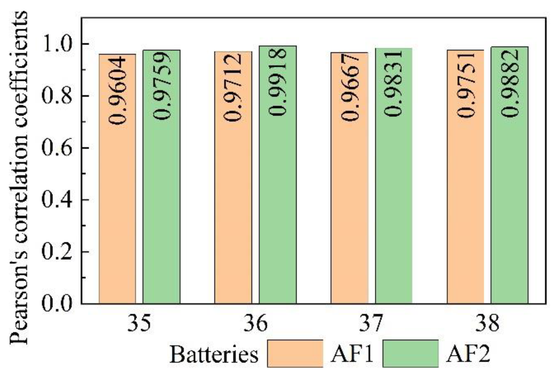
The Pearson’s correlation coefficients between the AFs and capacity are calculated by Pearson correlation analysis according to Equation (2), to evaluate the effectiveness of extracted Afs, and the results are shown Figure 3.
where and are the mean values of the AFs and capacity, respectively.
Based on Figure 3, it is significant for AFS to describe battery capacity degradation. Typically, a coefficient greater than 0.8 is considered strong, while a coefficient less than 0.5 is regarded as weak. In this case, the minimum value of obtained is 0.9604, indicating a strong correlation between the AFs and capacity degradation. Moreover, most of the values are approximately 0.98, further reinforcing the existence of a strong correlation between these variables. Additionally, the high correlation coefficients (>0.98) obtained between the ageing features suggest a strong coupling relationship between them. These results provide valuable insights into the understanding of battery ageing mechanisms and could have implications for the development of effective battery management strategies. Based on the ICC-based AFs, SOH estimation can be further carried out.
2.2. The Extrapolation of the Aging Features
For RUL prediction, the future aging trends need to be extrapolated standing on the historical measurable or estimated information. The modelling based on estimated information would introduce the predicted errors again, which leads to an inaccurate prediction of RUL. Herein, we try to model the measure AFs for extrapolation and RUL prediction.
The two AFs can be regarded as the monotone series, respectively; meanwhile, the cycle can be regarded as the time series. Thus, the monotonicity of AFs can be utilized to model and predict the growing trend. For this purpose, Pearson’s correlation coefficients are used to evaluate the relationship between the AFs and the cycle, and the results are illustrated in Figure 4.
Pearson’s correlation coefficient is a statistical measure that can quantify the degree of correlation between variables. The coefficients range from −1 to +1, and a greater coefficient implies a stronger correlation while the sign ± indicates the positive and negative correlation [36]. As shown in Figure 4, the coefficients are greater than 0.97. Such results suggest that there are strong linear relationships between the two AFs and cycles. In other words, linear fitting can be employed to model the trends between the AFs and cycle:
where and represent the two independent linear mappings. Herein, the least square method is utilized to determine the linear mapping based on the known data. However, the amount of online data increase gradually with battery age. The latest data need to be incorporated with the known data to establish linear mapping. Therefore, the mechanism of metabolism is introduced. The process of remodeling for AFs is shown in Figure 5:
As shown in Figure 5, the modelling can be implemented as follows:
(1) Based on the offline training data, the AFs and cycle are extracted as the dependent variable and independent variable, respectively. Then, the least square method is employed to model the relationships between cycle and AFs; furthermore, the parameterized mapping and are obtained.
(2) For a new battery, the cycle is defined as a sequence of real numbers that starts at 1. Then, the defined cycle is fed into the parameterized mapping and , the outputs of and are the two predicted AFs.
(3) When the battery is used, the measurable AFs and cycles are obtained. Combining the measurable data with the offline training data based on the metabolism, the new data are established. Then, the new data are employed to parameterize the , . With the continuous charging and discharging of the battery, the measurable AFs and cycles are used to reconstruct the modelling data continually.
Based on the predicted AFs, the further trend of battery degradation can be captured for RUL prediction.
3. Methodologies
As mentioned previously, AFs can be utilized to evaluate the current aging state and predict future degradation trends. How to establish a model for capturing the underlying relationship between AFs and capacity is an important factor in SOH estimation and RUL prediction. Herein, RF is employed to deal with this dilemma.
3.1. Random Forest Regression Optimization Model
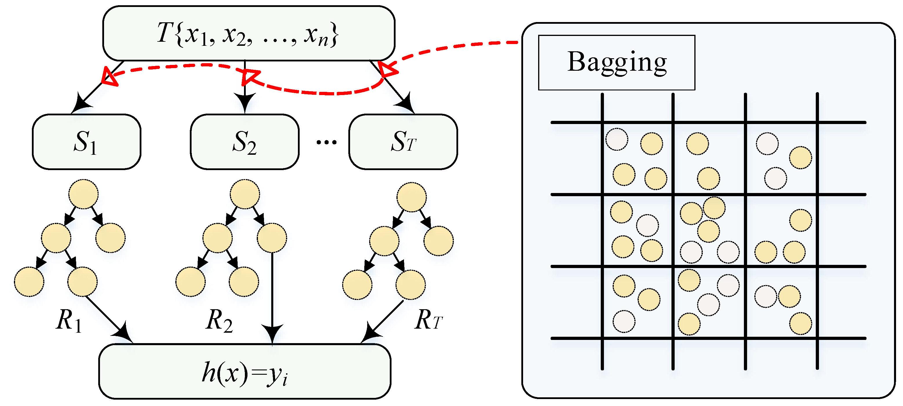
RF is a typical bagging-based ensemble learning method that combines multiple randomized decision trees and averages their outputs [37]. Through resampling the original data using the Bootstrap sampling method, a new training set is constructed to build a classification tree or regression tree for each new sample set using the CART method, as well as to provide the final prediction results according to the results of all of the decision trees. Compared with other machine learning algorithms, such as back propagation neural networks (BPNN) and SVR, RF exhibit superior scalability in processing large-scale high-dimensional data with fewer optimization parameters. Additionally, RF’s built-in estimation methods enhance the generalization ability of the prediction models, making it a more advantageous approach in machine learning. A schematic representation of the RF is depicted in Figure 6.
As shown in Figure 6, the implementation steps of planning for RF are as follows:
(1) Bootstrap is employed to resample the origin data, and then sample sets for training are obtained and labeled .
(2) The newly resampled training set is utilized to build the corresponding regression tree model . Prior to attribute selection for each internal node, attributes are randomly sampled from attributes, and the optimal splitting method among these attributes is employed to partition each node. The CART algorithm is utilized as the splitting method. It should be noted that, unlike the decision tree algorithm, there is no need to prune the CART. Finally, an RF model is determined.
(3) For unknown test samples, each regression tree can be used to calculate, and the corresponding predicted value of each regression tree can be obtained .
(4) The predicted values obtained from each individual regression tree are averaged and utilized as the final prediction outcome of the random forest model.
The new training set will not encompass all the data from the original training set because of Bootstrap. The excluded dataset is referred to as an out-of-bag (OOB) sample. Usually, a selection of two-thirds of the original training set samples is utilized to construct the regression function. The remaining data constitute the OOB sample, which is the new test set. The remaining data from the OOB sample are the new test set. Each time a regression tree is constructed using the new training set, the performance of the regression tree is evaluated by utilizing the OOB sample as a built-in cross-validation process. Thanks to this, the RF algorithm is capable of computing unbiased generalization errors without relying on unbiased estimation of such errors. The algorithm can also calculate unbiased estimates of generalization errors without using external data subsets. In addition, this built-in cross-validation feature enhances the ability to generalize RF algorithms using independent test data. In addition, this built-in cross-validation feature enhances the ability to generalize RF algorithms using independent test data. The error of OOB is calculated as follows:
where and are the predicted and true values of , respectively, and is the number of OOB samples.
Two of the most important hyperparameters in RF are necessary to determine the following: (1) The complexity (depth) of the trees in the forest. Deep trees tend to overfit, but shallow trees tend to underfit. (2) When growing the trees, the number of predictors to sample at each node. How to determine the hyperparameters plays a vital role in the prediction accuracy of RF to choose the best model.
3.2. Bayesian Optimization
An optimization algorithm assumes that the objective function is known to obtain the derivative and that the objective function is convex. Nonetheless, for some problems, in the parameter adjustment process, the objective function may not have a convex form, requiring heavy calculations and poor results. To solve such a problem, BO is developed. The core idea of BO is to leverage prior knowledge for approximating the posterior distribution of an unknown objective function, and subsequently selecting the next sampling hyperparameter combination based on this distribution [38]. To approach the objective function as closely as possible, the Bayesian algorithm adopts a proxy model, and the Gaussian process (GP) is often used to establish such a proxy model. With the GP algorithm, prior functions are defined that can be used to incorporate prior information about the objective function (smoothness, for example). BO is composed of two parts: a Bayesian statistical model is employed to represent the objective function, and an acquisition function is utilized to determine where to sample next. After conducting the initial space-filling experiment design, which typically involves selecting points uniformly at random to evaluate the target; these points are then iteratively utilized to allocate the remaining budget for N function evaluations. A typical pseudo-code of BO is shown in Algorithm 1:
| Algorithm 1: Bayesian optimization |
| for n=1, 2, …, do select new xn+1 by optimizing acquisition function α query objective function to obtain yn+1 update statistical model end for |
Based on BO, two optimal hyperparameters can be obtained; furthermore, an optimized RF can be trained to possess excellent abilities for learning and generalization. Then, the optimized RF can be utilized to capture the underlying correlation between AFs and capacity.
3.3. The Flowchart for SOH and RUL
According to the optimized RF model, a framework is established for estimating battery SOH and predicting RUL, as illustrated in Figure 7.
According to Figure 7, the process of SOH estimation and RUL prediction are described as follows:
(1) Online AFs extraction and prediction: (1) Based on the charging process, the online AFs are extracted to quantify the battery capacity degradation indirectly. Meanwhile, the correlation analysis is implemented to judge the effectiveness. (2) The historical and online AFs are modelled to predict the trends of AFs through extrapolation.
(2) Optimized random forest regression model: (1) According to the offline datasets, the original datasets are divided into a training set and testing set. (2) BO is employed to determine the optimal hyperparameters of RF based on the offline datasets. (3) The optimal hyperparameter is applied to RF, and an optimized RF model is trained.
(3) Model evaluation: (1) The online extracted AFs are fed into the optimized RF model to estimate battery capacity and calculate SOH. (2) The predicted AFs are simultaneously fed into the optimized RF model to predict the battery capacity and RUL.
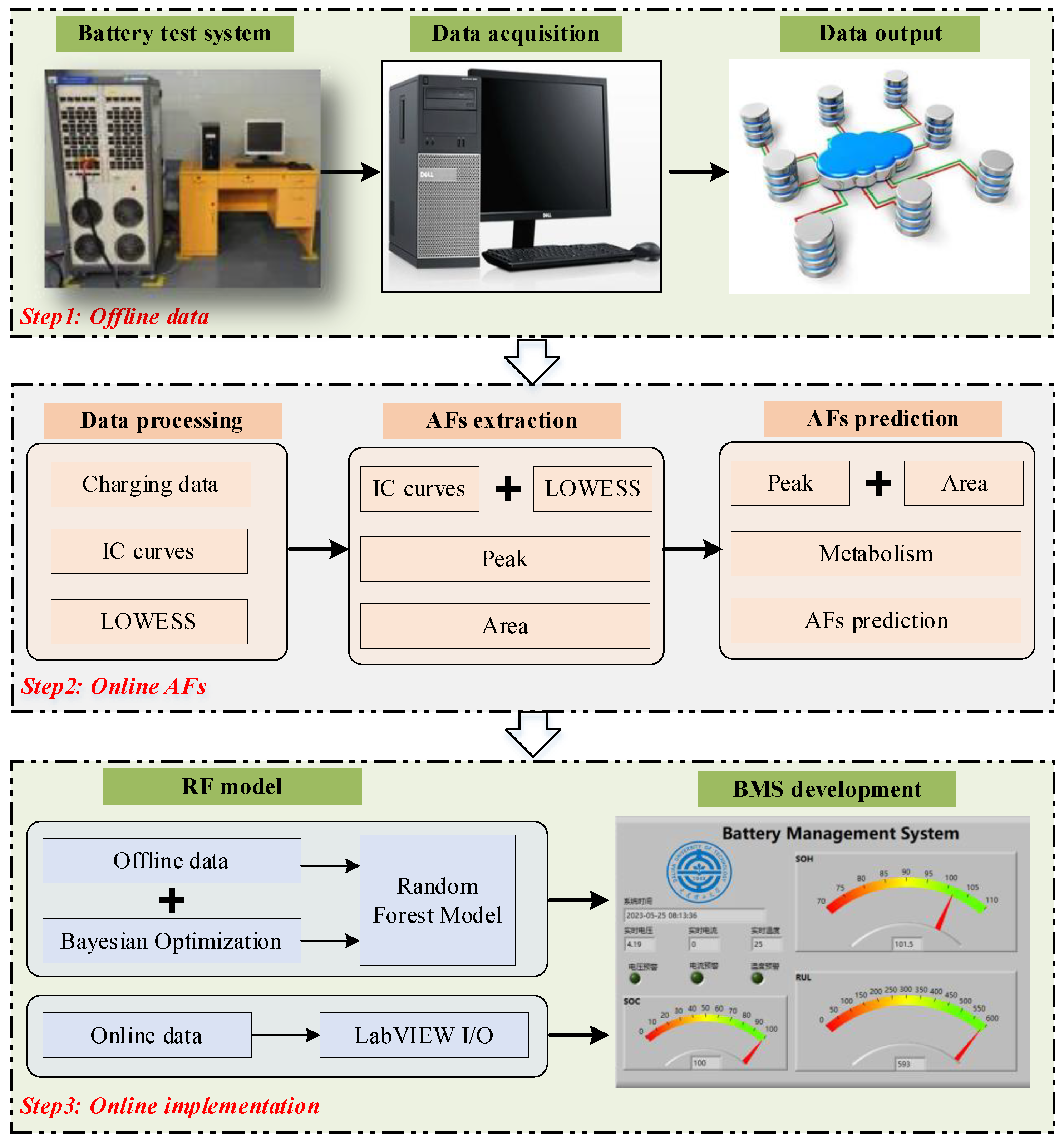
Furthermore, the embedded development of the flowchart for BMS is implemented based on hybrid programming through MATLAB and LabVIEW. MATLAB is regarded as the data processing center, while LabVIEW is used to acquire data and develop the human machine interface (HMI). In other words, MATLAB treats the online measurement information, trains the optimized RF model, and then estimates SOH and predicts RUL. The online information and the output are displayed on HMI by LabVIEW; meanwhile, the results are stored locally along with metadata. The interface of BMS is shown in Figure 8.
In Figure 8, BMS can be implemented through the following steps:
(1) Offline data acquisition: The charging and discharging of the battery are implemented through the Arbin battery test system.
(2) Online AFs extraction and prediction: Based on the online measurements, the online AFs are extracted, and then the future trends of AFs are predicted based on the online measurements and historical AFs.
(3) Online implementation: According to RF and BO, an optimal RF model is trained to capture the correlation between AFs and capacity. Furthermore, the RF model is embedded into LabVIEW for achieving online SOH estimation and RUL prediction based on the extracted AFs and predicted AFs. The results are shown in HMI and saved locally.
4. Results and Discussion
For the four batteries, batteries CS 36 and 38 are as the training datasets to obtain the optimized RF model for BMS development, while batteries CS 35 and 37 are as the test datasets for the validation of online SOH estimation and RUL prediction. Based on the developed BMS, the signal collection is implemented through the file I/O interface, and then the stored results of SOH estimation and RUL prediction for BMS are analyzed.
4.1. SOH Estimation
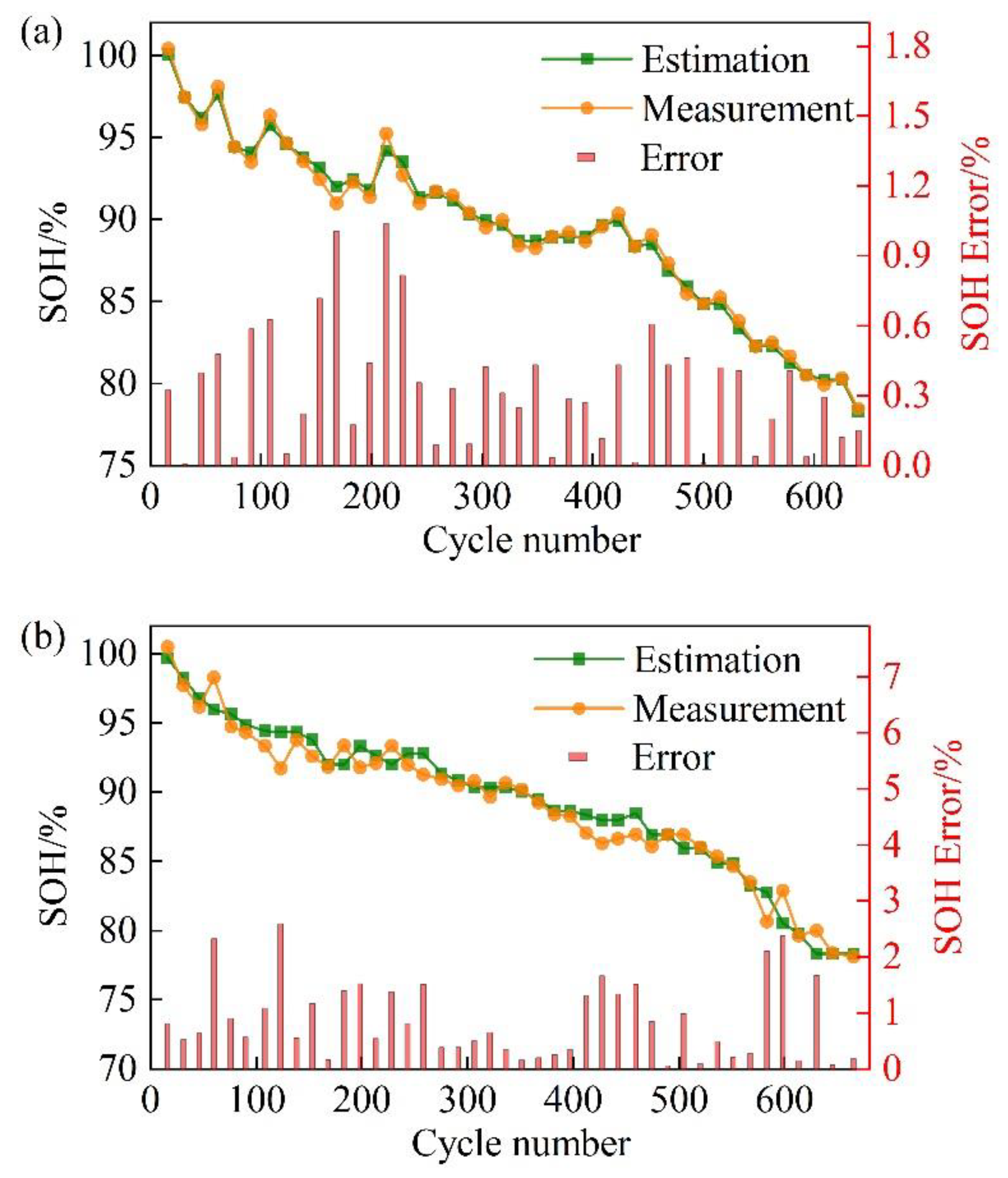
Taking the cycle number as the X axis, the SOH as the left Y axis, and the SOH error as the right Y axis, draw the curves of the measured and estimated SOH, shown in Figure 9, based on the results of SOH estimation.
Furthermore, the estimation error is analyzed from the different error evaluation indicators, encompassing the maximum absolute error (MAE) and root mean square error (RMSE), as illustrated in Equation (6):
where and are the true and estimated values, respectively; is the number of the sequence; and is the index of the sequence.
The result of the statistics is shown in Table 1.
(1) As the cycle increases, the battery SOH has a nonlinear decreasing tendency. In addition, the local battery capacity regeneration phenomenon plays a vital role in battery capacity degradation. The phenomenon brings great difficulty to accurate capacity tracking.
(2) The optimized RF model is capable of achieving precise battery SOH estimation. The estimated SOH has a high degree of coincidence with the measured SOH. However, the degree of deviation in the local capacity regeneration stage is greater than in the global degradation stage.
(3) From the perspective of SOH estimation error, the maximum MAE and RMSE for the two batteries are 2.5925 and 1.0976, respectively. In addition, the mean MAE and EMSE are 1.8152 and 0.7581, respectively, the mean MAE and RMSE suggest that the developed BMS can achieve accurate SOH estimation.
4.2. RUL Prediction
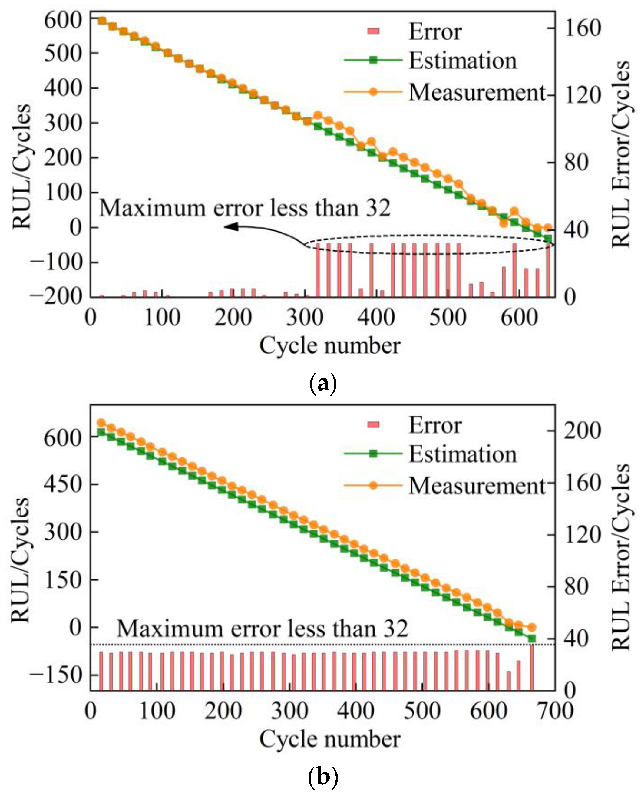
Similarly, taking the cycle number as the X axis, the RUL as the left Y axis, and the RUL error as the right Y axis, the curves of the measured and estimated SOH are drawn as shown in Figure 10 based on the results of RUL estimation.
Furthermore, the estimation error is analyzed from the different error evaluation indicators, consisting of MAE and RMSE. The results of the statistics are shown in Table 2.
(1) As the cycle increases, RUL continues to gradually decline. Combined with the definition of RUL, there is a significant negative linear correlation between the number of cycles and the measured RUL.
(2) The predicted RUL can track the measured RUL, and the predicted curves vibrate around the true RUL. In addition, the differences between the measured and predicted RUL remain basically unchanged during the full life cycle. According to the predicted RUL, the developed BMS can achieve continuous RUL prediction.
(3) In the whole prediction process, the maximum MAE and RMSE for the two batteries are 32 and 29.3198 cycles. Furthermore, the mean MAE and RMSE are 32 and 24.8580 cycles, respectively. Comparatively speaking, the developed BMS can predict the RUL with a high accuracy continuously.
4.3. Discussion
For providing a fair performance comparison, different methods are implemented for SOH estimation and RUL prediction with the same framework; herein, the traditional BP neural network (BPNN) with a single hidden layer, 20 nodes, and a Sigmoid activation function [39]; SVM with a radial basis kernel function [35]; and RF without optimization are selected. Meanwhile, the means of evaluation indexes for the two batteries are calculated, and the results are shown in Table 3.
According to the results shown in Table 3, the mean MAEs of SOH estimation for the three methods are 2.6138, 3.1786, and 2.7293, and the mean RMSEs are 1.0838, 1.3333, and 1.1627; for RUL prediction, the mean MAEs are about 33.5, while the mean RMSEs are 28.2835, 33.5, and 30.6125. Relatively speaking, BPNN has the best performance for the SOH estimation and RUL prediction in the three methods; however, the results are still worse than the proposed optimization model. Especially, RF without optimization cannot determine the appropriate hyperparameters; thus, the estimation or prediction performance is lower than the RF optimization model.
To sum up, the excellent SOH estimation and RUL prediction suggest that the developed optimized RF model and BMS can achieve the effective online application of PHM. As the main components of the framework, the embedded method for BMS plays a crucial role.
(1) The bagging is employed in RF to avoid the correlation among multiple decision trees. Furthermore, the diversity of the trees can be improved by constructing different subsets of training data. Therefore, the RF model becomes more robust to slight variations in input data due to greater stability by utilizing bagging; also, bagging reduces noise through generating non-correlated trees using different training samples.
(2) It is necessary for the RF model to only tune two hyperparameters. Herein, BO is effective at addressing optimization problems where the objective function is unknown or a black-box function. BO amalgamates the function’s prior distribution with the sample information (evidence) to derive the function’s posterior property, and subsequently employs this information to ascertain the optimal position of the said function based on predetermined criteria. Therefore, in a small number of samples, BO can achieve high accuracy in a short time.
(3) The development of co-simulation using LabVIEW and MATLAB for verification of the optimized RF model is carried out. Based on BMS, the co-simulation technology brings about a new idea to implement the simulation of the hardware in the loop.
5. Conclusions
In this study, an optimized RF model is developed for online SOH estimation and RUL prediction, as follows:
(1) Based on the partial charging data, two ICC-based AFs are extracted. In addition, the AFs are proven to have a strong correlation with battery capacity and quantify the battery capacity degradation.
(2) An RF model is developed to capture the underlying relationship between battery capacity and AFs. Meanwhile, BO is employed to determine the hyperparameters of the RF model, in order to obtain an optimized RF model.
(3) The developed RF optimization model is deployed through co-simulation using LabVIEW and MATLAB for online SOH estimation and RUL prediction. The aging datasets are employed to validate the effectiveness of the proposed method with an average SOH estimation error of less than 1.8152% and an average RUL prediction error of less than 32 cycles.
This work does not take into account the influence of the different temperature and the failure thresholds. In future work, we will pay more attention to the temperature and threshold variations. On the other hand, the digitally controlled power supply embedded in the RF optimization model will be used to develop an estimator in the charger for online estimation of battery in-loop capacity under more uncontrolled environmental factors. Meanwhile, the echelon utilization of the retired EVs needs to be researched.
Author Contributions
G.W. conceived the idea of SOH estimation, led and supervised the project, and participated in paper writing and revision. Z.L. and X.L. supervised and led the project. All of the authors have revised the manuscript and agreed with its content. All authors have read and agreed to the published version of the manuscript.
Funding
This research was funded by the doctoral research project of Anhui University.
Data Availability Statement
The data presented in this study are openly available in https://calce.umd.edu/battery-data (accessed on 20 May 2023).
Conflicts of Interest
The authors declare no conflict of interest.
Nomenclature
| EV | Electric vehicle |
| PHM | Prognostics and health management |
| SOH | State of health |
| RUL | Remaining useful life |
| EM | Electrochemical model |
| ECM | Equivalent circuit model |
| PF | Particle filter |
| SOC | State of charge |
| EKF | Extended Kalman filter |
| AF | Aging feature |
| BO | Bayesian optimization |
| BMS | Battery management system |
| RF | Random forest |
| SVR | Support vector regression |
| EIS | Electrochemical impedance spectroscopy |
| RVM | Relevance vector machine |
| ELM | Extreme learning machine |
| ICC | Incremental capacity curve |
| ICA | Incremental capacity analysis |
| PSO | Particle swarm optimization |
| LOWESS | Locally weighted scatterplot smoothing |
| PICC | Peak of the incremental capacity curve |
| CCEV | Charged capacity of equal voltage |
| BPNN | Back propagation neural networks |
References
- Li, X.; Yuan, C.; Wang, Z.; He, J.; Yu, S. Lithium battery state-of-health estimation and remaining useful lifetime prediction based on non-parametric aging model and particle filter algorithm. eTransportation 2022, 11, 100156. [Google Scholar] [CrossRef]
- Yu, Q.; Huang, Y.; Tang, A.; Wang, C.; Shen, W. Ocv-soc-temperature relationship construction and state of charge estimation for a series—parallel lithium-ion battery pack. IEEE Trans. Intell. Transp. Syst. 2023, 24, 6362–6371. [Google Scholar] [CrossRef]
- Guo, Y.; Yang, D.; Zhao, K.; Wang, K. State of health estimation for lithium-ion battery based on bi-directional long short-term memory neural network and attention mechanism. Energy Rep. 2022, 8, 208–215. [Google Scholar] [CrossRef]
- Yu, Q.; Liu, Y.; Long, S.; Jin, X.; Li, J.; Shen, W. A branch current estimation and correction method for a parallel connected battery system based on dual bp neural networks. Green Energy Intell. Transp. 2022, 1, 100029. [Google Scholar] [CrossRef]
- Lin, D.; Zhang, X.; Wang, L.; Zhao, B. State of health estimation of lithium-ion batteries based on a novel indirect health indicator. Energy Rep. 2022, 8, 606–613. [Google Scholar] [CrossRef]
- Wang, C.; Yu, C.; Guo, W.; Wang, Z.; Tan, J. Identification of typical sub-health state of traction battery based on a data-driven approach. Batteries 2022, 8, 65. [Google Scholar] [CrossRef]
- Zhao, J.; Burke, A.F. Electric vehicle batteries: Status and perspectives of data-driven diagnosis and prognosis. Batteries 2022, 8, 142. [Google Scholar] [CrossRef]
- Wang, H.; Li, J.; Liu, X.; Rao, J.; Fan, Y.; Tan, X. Online state of health estimation for lithium-ion batteries based on a dual self-attention multivariate time series prediction network. Energy Rep. 2022, 8, 8953–8964. [Google Scholar] [CrossRef]
- Wang, Z.; Feng, G.; Zhen, D.; Gu, F.; Ball, A. A review on online state of charge and state of health estimation for lithium-ion batteries in electric vehicles. Energy Rep. 2021, 7, 5141–5161. [Google Scholar] [CrossRef]
- Wang, S.; Jin, S.; Bai, D.; Fan, Y.; Shi, H.; Fernandez, C. A critical review of improved deep learning methods for the remaining useful life prediction of lithium-ion batteries. Energy Rep. 2021, 7, 5562–5574. [Google Scholar] [CrossRef]
- Hu, X.; Jiang, J.; Cao, D.; Egardt, B. Battery health prognosis for electric vehicles using sample entropy and sparse bayesian predictive modeling. IEEE Trans. Ind. Electron. 2016, 63, 2645–2656. [Google Scholar] [CrossRef]
- Kuipers, M.; Schröer, P.; Nemeth, T.; Zappen, H.; Blömeke, A.; Sauer, D.U. An algorithm for an online electrochemical impedance spectroscopy and battery parameter estimation: Development, verification and validation. J. Energy Storage 2020, 30, 101517. [Google Scholar] [CrossRef]
- Li, J.; Adewuyi, K.; Lotfi, N.; Landers, R.G.; Park, J. A single particle model with chemical/mechanical degradation physics for lithium ion battery state of health (soh) estimation. Appl. Energy 2018, 212, 1178–1190. [Google Scholar] [CrossRef]
- Du, X.; Meng, J.; Zhang, Y.; Huang, X.; Wang, S.; Liu, P.; Liu, T. An information appraisal procedure: Endows reliable online parameter identification to lithium-ion battery model. IEEE Trans. Ind. Electron. 2022, 69, 5889–5899. [Google Scholar] [CrossRef]
- Bi, Y.; Yin, Y.; Choe, S. Online state of health and aging parameter estimation using a physics-based life model with a particle filter. J. Power Sources 2020, 476, 228655. [Google Scholar] [CrossRef]
- Allam, A.; Onori, S. Online capacity estimation for lithium-ion battery cells via an electrochemical model-based adaptive interconnected observer. IEEE Trans. Control Syst. Technol. 2021, 29, 1636–1651. [Google Scholar] [CrossRef]
- Yu, Q.; Dai, L.; Xiong, R.; Chen, Z.; Zhang, X.; Shen, W. Current sensor fault diagnosis method based on an improved equivalent circuit battery model. Appl. Energy 2022, 310, 118588. [Google Scholar] [CrossRef]
- Zou, Y.; Hu, X.; Ma, H.; Li, S.E. Combined state of charge and state of health estimation over lithium-ion battery cell cycle lifespan for electric vehicles. J. Power Sources 2015, 273, 793–803. [Google Scholar] [CrossRef]
- Lyu, Z.; Gao, R. A model-based and data-driven joint method for state-of-health estimation of lithium-ion battery in electric vehicles. Int. J. Energy Res. 2019, 43, 7956–7969. [Google Scholar] [CrossRef]
- Vanem, E.; Salucci, C.B.; Bakdi, A.; Alnes, Ø.Å.S. Data-driven state of health modelling—A review of state of the art and reflections on applications for maritime battery systems. J. Energy Storage 2021, 43, 103158. [Google Scholar] [CrossRef]
- Hamar, J.C.; Erhard, S.V.; Canesso, A.; Kohlschmidt, J.; Olivain, N.; Jossen, A. State-of-health estimation using a neural network trained on vehicle data. J. Power Sources 2021, 512, 230493. [Google Scholar] [CrossRef]
- Pradyumna, T.K.; Cho, K.; Kim, M.; Choi, W. Capacity estimation of lithium-ion batteries using convolutional neural network and impedance spectra. J. Power Electron. 2022, 22, 850–858. [Google Scholar] [CrossRef]
- Zhang, W.; Li, X.; Li, X. Deep learning-based prognostic approach for lithium-ion batteries with adaptive time-series prediction and on-line validation. Measurement 2020, 164, 108052. [Google Scholar] [CrossRef]
- Pan, W.; Luo, X.; Zhu, M.; Ye, J.; Gong, L.; Qu, H. A health indicator extraction and optimization for capacity estimation of li-ion battery using incremental capacity curves. J. Energy Storage 2021, 42, 103072. [Google Scholar] [CrossRef]
- Wu, J.; Fang, L.; Meng, J.; Lin, M.; Dong, G. Optimized multi-source fusion based state of health estimation for lithium-ion battery in fast charge applications. IEEE Trans. Energy Convers. 2022, 37, 1489–1498. [Google Scholar] [CrossRef]
- Duong, P.L.T.; Raghavan, N. Heuristic kalman optimized particle filter for remaining useful life prediction of lithium-ion battery. Microelectron. Reliab. 2018, 81, 232–243. [Google Scholar] [CrossRef]
- Wei, J.; Dong, G.; Chen, Z. Remaining useful life prediction and state of health diagnosis for lithium-ion batteries using particle filter and support vector regression. IEEE Trans. Ind. Electron. 2018, 65, 5634–5643. [Google Scholar] [CrossRef]
- Downey, A.; Lui, Y.; Hu, C.; Laflamme, S.; Hu, S. Physics-based prognostics of lithium-ion battery using non-linear least squares with dynamic bounds. Reliab. Eng. Syst. Saf. 2019, 182, 1–12. [Google Scholar] [CrossRef]
- Liu, Q.; Zhang, J.; Li, K.; Lv, C. The remaining useful life prediction by using electrochemical model in the particle filter framework for lithium-ion batteries. IEEE Access 2020, 8, 126661–126670. [Google Scholar] [CrossRef]
- Hu, X.; Xu, L.; Lin, X.; Pecht, M. Battery lifetime prognostics. Joule 2020, 4, 310–346. [Google Scholar] [CrossRef]
- Afshari, S.S.; Cui, S.; Xu, X.; Liang, X. Remaining useful life early prediction of batteries based on the differential voltage and differential capacity curves. IEEE Trans. Instrum. Meas. 2022, 71, 6500709. [Google Scholar] [CrossRef]
- Feng, H.; Song, D. A health indicator extraction based on surface temperature for lithium-ion batteries remaining useful life prediction. J. Energy Storage 2021, 34, 102118. [Google Scholar] [CrossRef]
- Yao, F.; He, W.; Wu, Y.; Ding, F.; Meng, D. Remaining useful life prediction of lithium-ion batteries using a hybrid model. Energy 2022, 248, 123622. [Google Scholar] [CrossRef]
- Lyu, Z.; Gao, R.; Li, X. A partial charging curve-based data-fusion-model method for capacity estimation of li-ion battery. J. Power Sources 2021, 483, 229131. [Google Scholar] [CrossRef]
- Li, X.; Yuan, C.; Wang, Z. State of health estimation for li-ion battery via partial incremental capacity analysis based on support vector regression. Energy 2020, 203, 117852. [Google Scholar] [CrossRef]
- Lyu, Z.; Wang, G.; Gao, R. Synchronous state of health estimation and remaining useful lifetime prediction of li-ion battery through optimized relevance vector machine framework. Energy 2022, 251, 123852. [Google Scholar]
- Li, Y.; Zou, C.; Berecibar, M.; Nanini-Maury, E.; Chan, J.C.W.; van den Bossche, P.; Van Mierlo, J.; Omar, N. Random forest regression for online capacity estimation of lithium-ion batteries. Appl. Energy 2018, 232, 197–210. [Google Scholar] [CrossRef]
- Wu, J.; Chen, X.; Zhang, H.; Xiong, L.; Lei, H.; Deng, S. Hyperparameter optimization for machine learning models based on bayesian optimizationb. J. Electron. Sci. Technol. 2019, 17, 26–40. [Google Scholar]
- Lin, H.; Kang, L.; Xie, D.; Linghu, J.; Li, J. Online state-of-health estimation of lithium-ion battery based on incremental capacity curve and bp neural network. Batteries 2022, 8, 29. [Google Scholar] [CrossRef]
Figure 1.
The smoothing results of ICC.

Figure 2.
The smoothing results of ICC.

Figure 3.
The smoothing results of ICC.

Figure 4.
Pearson’s correlation coefficients.

Figure 5.
The modelling of metabolism.

Figure 6.
The schematic diagram of the RF.

Figure 7.
The framework for battery SOH estimation and RUL prediction.

Figure 8.
BMS for online battery SOH estimation and RUL prediction.

Figure 9.
BMS for online battery SOH estimation and SOH prediction: (a) CS35 and (b) CS37.

Figure 10.
BMS for online battery RUL estimation and RUL prediction: (a) CS35 and (b) CS37.


Table 1.
Error analysis of SOH estimation.
| Index | MAE (%) | RMSE |
|---|---|---|
| CS 35 | 1.0379 | 0.4185 |
| CS 37 | 2.5925 | 1.0976 |
| Mean | 1.8152 | 0.7581 |
Table 2.
Error analysis of RUL prediction.
| Index | MAE (Cycle) | RMSE |
|---|---|---|
| CS 35 | 32 | 20.3961 |
| CS 37 | 32 | 29.3198 |
| Mean | 32 | 24.8580 |
Table 3.
Error comparison analysis.
| Batteries | Index | Mean MAE | Mean RMSE |
|---|---|---|---|
| BPNN | SOH estimation | 2.6138 | 1.0838 |
| RUL prediction | 33.5 | 28.2835 | |
| SVM | SOH estimation | 3.1786 | 1.3333 |
| RUL prediction | 33.5 | 33.5 | |
| RF | SOH estimation | 2.7293 | 1.1627 |
| RUL prediction | 33.5 | 30.6125 |
Disclaimer/Publisher’s Note: The statements, opinions and data contained in all publications are solely those of the individual author(s) and contributor(s) and not of MDPI and/or the editor(s). MDPI and/or the editor(s) disclaim responsibility for any injury to people or property resulting from any ideas, methods, instructions or products referred to in the content. |
© 2023 by the authors. Licensee MDPI, Basel, Switzerland. This article is an open access article distributed under the terms and conditions of the Creative Commons Attribution (CC BY) license (https://creativecommons.org/licenses/by/4.0/).
Share and Cite
MDPI and ACS Style
Wang, G.; Lyu, Z.; Li, X. An Optimized Random Forest Regression Model for Li-Ion Battery Prognostics and Health Management. Batteries 2023, 9, 332. https://doi.org/10.3390/batteries9060332
AMA Style
Wang G, Lyu Z, Li X. An Optimized Random Forest Regression Model for Li-Ion Battery Prognostics and Health Management. Batteries. 2023; 9(6):332. https://doi.org/10.3390/batteries9060332
Chicago/Turabian StyleWang, Geng, Zhiqiang Lyu, and Xiaoyu Li. 2023. "An Optimized Random Forest Regression Model for Li-Ion Battery Prognostics and Health Management" Batteries 9, no. 6: 332. https://doi.org/10.3390/batteries9060332
Note that from the first issue of 2016, this journal uses article numbers instead of page numbers. See further details here.