Non-Interferometric Tomography of Phase Objects Using Spatial Light Modulators

Abstract

Quantitative 3D phase retrieval techniques are based on either interferometric techniques such as holography or noninterferometric intensity-based techniques such as the transport of intensity equation (TIE). Interferometric techniques are vibration-sensitive and often use a reference beam requiring complicated optical alignment. In this work we develop a simple, fast, and noninterferometric tomographic 3D phase retrieval technique based on the TIE which does not suffer from such drawbacks. The optical setup is a modified 4f TIE system which uses an SLM to replace the slow translation of the CCD required to record several diffraction patterns in a traditional TIE system. This novel TIE setup is suitable for dynamical events such as imaging biological processes. A rotating mechanical stage is constructed to obtain tomographic phase images of the object. The tomographic reconstruction algorithm is based on the Fourier slice theorem (backprojection algorithm) which applies to objects with a small refractive index span. Simulation and experimental results are shown as part of this work. A graphical user interface is developed to perform the TIE tomographic reconstruction algorithm and to synchronize the captured intensities by the CCD, the phase patterns displayed on the SLM, and the Arduino controlled rotating stage assembly.

1. Introduction

To be visible to imaging modalities, a phase object should have a different shape and/or refractive index with respect to its surroundings. Exploiting these variations is crucial to predict and visualize several biological objects, processes, and track their movements and interactions. This is especially important in the biological study of cells, which are nearly undetectable in bright field microscopy but exhibit strong phase contrast. Hence, acquiring phase information is very crucial. There exist many phase contrast techniques to obtain phase information, such as phase-contrast (PC) microscopy [1] and differential interference contrast (DIC) microscopy [2]. These methods, however, have some limitations such as thickness of the sample, distortion, prerequisite orientation, shade-off effect, insufficient internal details, challenging to interpret of cell structure, halo effects, unsuitability for non-biological uses, and above all requiring complicated expensive equipment.

For the last several decades, efficient label-free phase retrieval techniques used for 3D image reconstruction has been the subject of enormous amount of research. These techniques are primarily divided into two main categories: interferometric based techniques such as digital holography [3,4,5,6,7] and noninterferometric techniques such as the transport of intensity (TIE) [8,9,10,11,12,13,14,15,16,17] and ptychography [18,19,20].

Interferometric phase retrieval techniques are extremely accurate, but are sensitive to vibrations, thus, requiring vibration isolation stages and more fit to a laboratory environment. In addition, interferometric techniques often require coherent sources that rely on the interference between a reference and an object beam, although some interferometric techniques based on partially coherent sources using the mutual intensity has recently emerged [21,22,23]. Noninterferometric phase retrieval techniques, such as TIE-based systems, have obvious advantages over interferometric techniques. TIE-based systems are simple to construct, immune to vibrations, no phase unwrapping is needed, and can be employed with partially coherent sources [8,9,10,11,12,13,14,15,16,17]. The phase retrieval in a TIE system is based on the relationship between the derivative of intensity along the propagation direction and the phase of the propagating beam. Hence, the phase can be indirectly computed by recording multiple intensity images on a recording device such as a CCD. In a traditional TIE setup, a CCD is translated along the propagation direction recording multiple defocused intensity patterns. The drawbacks of a TIE phase retrieval system are the need for an accurate (no drift in the lateral dimensions) and slow mechanical translation [3,4]. Ptychography is another label-free, high contrast, and intensity-based technique that uses a set of diffraction patterns to create an image of a specimen using phase retrieval algorithms. There remains a huge amount of work to be accomplished in both improving the inversion algorithms that are required to invert the data and reconstruct the image and for optimizing the experimental configurations used for ptychography [18,19,20]. In a previous work, an electrically tunable liquid crystal lens (ETL) with a variable focal length was employed in the TIE system to mimic diffraction and serves to replace the mechanical translation of the CCD camera [14,24]. This system has many advantages since it resulted in faster acquisition of the intensity patterns and it is immune to translational misalignment noise of the CCD camera making it more suitable to record dynamical events. Also, the derivative estimation was improved because of the ability of the system to capture multiple intensity images at different planes in a short period of time, thus reducing the error in the derivative estimation. Thus, one can construct a fully automated 360-degree field of view 4f tomographic TIE system using a tunable lens [24,25]. Although the ETL-TIE system is superior in acquisition time and more immune to noise, the speed of the overall system is controlled by the speed of the electrically tunable lens.

In this work, a spatial light modulator (SLM) is employed in a tomographic 360-degree TIE setup to mimic diffraction instead of the traditional mechanical translation or the electrically tunable lens based TIE system. A non-tomographic SLM-based TIE system provides the integration along the optical path and is not suited to render a full view 3D image [26]. In this work, tomographic capability is added to the SLM-based TIE setup through a custom-built rotation mechanism controlled by an Arduino microcontroller. Moreover, the theory behind the equivalence of the SLM-based setup and the traditional TIE setup is developed. A relation between the SLM pattern focal length and axial translation is derived. A detailed analysis of the 3D tomographic reconstruction algorithm using the Fourier Slice theorem on TIE obtained simulated phase images is also developed [4,24,27,28]. Using the Fourier Slice theorem applied to weakly scattering objects (a small refractive index span that assumes that light propagates along straight lines within the sample) immersed in matching index liquid, experimental tomographic reconstruction results are also obtained. Although, there is no dispute that optical diffraction tomography using backpropagation gives more accurate results, in general, at the expense of more computation complexity, in the case of weakly scattering objects considered in this study the difference is not significant. Finally, a graphical user interface using MATLAB^® is developed to perform the TIE tomographic reconstruction algorithm and to synchronize the captured intensities by the CCD camera, the phase patterns displayed on the SLM, and the Arduino controlled rotating stage holding the object.

2. Brief Theory of the Transport of Intensity Phase Reconstruction Algorithm

The starting point in deriving the TIE is from the Helmholtz equation which can be written as:

$${\nabla }^{2}E\left(x,y,z\right)+k_0^{2}E\left(x,y,z\right)= 0,$$

(1)

where $E\left(x,y,z\right)$ is the complex wave field, $k_0=2\pi /{\lambda }_0$ is the wave number, ${\lambda }_0$ is the wavelength of illumination source, and ${\nabla }^2=\left(\frac{{\partial }^2}{\partial x^2}+\frac{{\partial }^2}{\partial y^2}+\frac{{\partial }^2}{\partial z^2}\right)$ is the Laplacian operator. Let $E\left(x,y,z\right)=E_e\left(x,y,z\right)\exp \left(-j{k}_{0}z\right)$, and under the paraxial approximation, substituting E into Equation (1) leads to

$$\frac{1}{2j{k}_0}{\nabla }_{\perp }^2{E}_e=\frac{\partial E_e}{\partial z}.$$

(2)

where ${\nabla }_{\perp }^2=\left(\frac{{\partial }^2}{\partial x^2}+\frac{{\partial }^2}{\partial y^2}\right)$ is the transverse Laplacian operator and $E_e$ is the envelope of the complex wave field. Since the envelop of the complex field can be written as $E_e\left(x,y,z\right)= \sqrt{I\left(x,y,z\right)}\exp \left(-j\phi \left(x,y,z\right)\right),$ substituting $E_e$ into Equation (2), will lead to the generic TIE

$${\overrightarrow{\nabla }}_{\perp }.\left[I\left(x,y\right){\overrightarrow{\nabla }}_{\perp }\phi \left(x,y\right)\right]=-k_0\frac{\partial I\left(x,y\right)}{\partial z} ,$$

(3)

where ${\overrightarrow{\nabla }}_{\perp }=\left(\frac{\partial }{\partial x},\frac{\partial }{\partial y}\right)$ is the gradient operator in the transverse dimensions over the propagation direction z. Hence, under paraxial approximation the TIE can be derived from the imaginary part of the Helmholtz equation [4,8,29]. Note that the left side of the TIE given by Equation (3) which contains information about the phase of the object is related to the right side of the same equation which contains information about the derivative of the intensity along the propagation direction.

In this work we study weak phase objects where the intensity $I\left(x,y,z_0\right)$ at a certain transverse plane $z_0$ is approximately constant. Equation (3) can then be approximated as:

$${\nabla }_{\perp }^2 \phi \left(x,y\right)=-\frac{k_0}{I\left(x,y\right)}\frac{\partial I\left(x,y\right)}{\partial z}.$$

(4)

The phase of the object at the CCD can be obtained by solving Equation (4) using the 2D spatial Fourier transform $\mathfrak{F}$ which leads to:

$${\phi }_{CCD}\left(x,y;z\right)={\mathfrak{F}}^{-1}\left\{{\Phi }_{CCD}\left(k_x.k_y;z\right)\right\}={\mathfrak{F}}^{-1}\left\{- k_0\frac{\mathfrak{F}\left\{\frac{1}{I_0\left(x,y\right)}\frac{\partial I\left(x,y\right)}{\partial z}\right\}}{k_x^2+k_y^2+a}\right\},$$

(5)

where $\frac{\partial I\left(x,y\right)}{\partial z}\approx \frac{I_{OF}\left(x,y\right)-I_{UF}\left(x,y\right)}{∆z}$, $I_0\left(x,y\right)$ is the intensity image at the focused image plane, $k_x.k_y$ denote the transverse spatial frequencies, $∆z$ is the defocused distance between the over-focused $I_{OF}\left(x,y\right)$ and the under-focused $I_{UF}\left(x,y\right)$intensity images captured on symmetrically located planes around the image plane, and $a$ is a regularization parameter used to optimize the results by ignoring the residual low frequency variations effect of the $\frac{1}{k_x^2+k_y^2}$ term, as shown in Figure 1a [17,30,31]. There exist two competing factors that should be considered for choosing the defocusing distance ∆z. If the defocusing distance is very small, the measurement noise might exceed the difference between the intensity distributions at the two defocused planes. If the defocusing distance is large, the signal will be less affected by measurement noise error. However, the estimate of the derivative according to Equation (5) becomes less accurate. Hence, the distance ∆z has to be correctly estimated to obtain accurate results. In a separate work a strategy has been developed to properly select the defocusing distance separating these two planes to correctly estimate the derivative of the intensity along the propagation direction z [32].

A traditional TIE optical setup consists of a 4f configuration (distance between L₁ and L₂ is equal to the summation of their focal lengths) as shown in Figure 1b. In this setup the object and the image planes are situated at the front and back focal planes of lens L₁ and L₂, respectively. In this system the CCD is translated at least two times to capture the intensity patterns required to estimate the derivative in Equation (5). A major drawback of such a system is the need of an accurate mechanical axial translation within a subpixel error lateral shift. This mechanical translation makes the traditional TIE system unsuitable for studying dynamical processes and events. 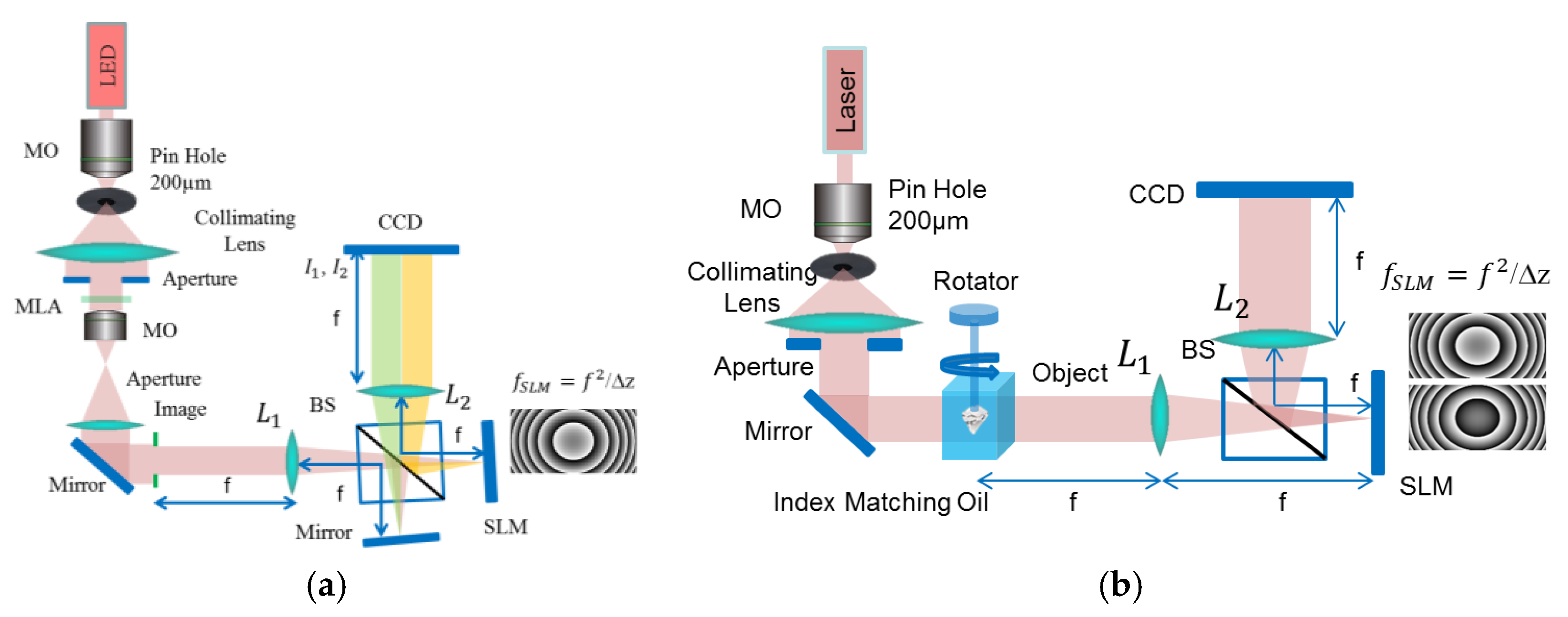This drawback can be mitigated by displaying a phase pattern on a spatial light modulator (SLM) situated at the back focal plane of L₁ to mimic the CCD translation, as described in Figure 2 [26].

Figure 2a shows a single-shot 4f TIE optical microscopy setup using an SLM and a mirror. In this setup half of the CCD will hold the diffraction from the mirror and the other half from the SLM. This setup works perfectly with small microscopic objects. Figure 2b shows a sequential recording 4f TIE optical microscopy setup with custom fabricated rotating stage assembly for full-view 360 degrees tomography of large phase objects. Both these setups are studied in this work. The SLM is a reflective liquid crystal on silicon (LCoS) phase-only modulator (Pluto, 1920 × 1080 pixels with 8 μm pixel size from Holoeye). The SLM is controlled from the developed GUI to provide full 2π phase modulation with linear electro-optical characteristic. A certain quadratic phase pattern is displayed on the SLM corresponding to the free space propagation transfer function. The following derivation shows that the SLM’s role in the TIE system is equivalent to the translation of the CCD by the axial defocusing distance ∆z. Consider an object denoted by $t\left(x,y\right)$ and placed at the front focal plane of lens L₁ of the 4f TIE system. A plane wave illuminating the object will result in a complex field at the back focal plane of lens L₂ which is a scaled version of the Fourier transform of the object. This complex field just before hitting the SLM can be written as: $\mathfrak{F}\left\{t\left(x,y\right)\right\}=T\left(k_x,k_y\right){|}_{\begin{array}{c}{k}_x= k_{0}x/f\\ k_y=k_{0}y/f\end{array}}$, where f is the focal length of L₁ or L₂ as shown in the setup of Figure 2. Displaying a quadratic phase pattern $s_{f_{SLM}}\left(x,y\right)= e^{\frac{j{k}_0\left(x^2+y^2\right)}{2f_{SLM}}}$ on the SLM (similar to a lens phase transformation function), the complex field just after the SLM can be expressed as:

$${u\left(x,y\right)|}_{\begin{array}{c}After\\ SLM\end{array}}=T\left(k_x,k_y\right){|}_{\begin{array}{c}{k}_x= k_{0}x/f\\ k_y=k_{0}y/f\end{array}}.s_{f_{SLM}}\left(x,y\right).$$

(6)

By the same token, the complex field $w\left(x,y\right)$ at the back focal plane of lens L₂ (CCD plane) is also the ${\mathfrak{F}\left\{u\left(x,y\right)\right\}|}_{\begin{array}{c}{k}_x= k_{0}x/f\\ k_y=k_{0}y/f\end{array}}$, and can be expressed as:

$${w_{SLM}\left(x,y\right)|}_{\begin{array}{c}Back focal\\ plane of L2\end{array}}={\mathfrak{F}\left\{T\left(k_x,k_y\right)\right\}|}_{\begin{array}{c}{k}_x= k_{0}x/f\\ k_y=k_{0}y/f\end{array}}*S_{f_{SLM}}\left(k_x,k_y\right) {|}_{\begin{array}{c}{k}_x= k_{0}x/f\\ k_y=k_{0}y/f\end{array}},$$

(7)

where $(*)$ denotes convolution and $S_{f_{SLM}}\left(k_x,k_y\right)=\mathfrak{F}\left\{s_{f_{SLM}}\left(x,y\right)\right\}$. After some straight forward algebra, Equation (7) can be simplified to:

$${w_{SLM}\left(x,y\right)|}_{CCD} \propto t\left(-x,-y\right)*e^{-j\frac{k_0{f}_{SLM}}{2f^2}\left(x^2+y^2\right)}.$$

(8)

In the traditional TIE optical setup where the SLM is not used, the complex field at the back focal plane of lens L₂ (CCD plane) can be expressed as [24]:

$${w\left(x,y\right)|}_{CCD} \propto t\left(-x,-y\right).$$

(9)

According to the Fresnel diffraction theory, the complex field on a plane at a defocused distance ∆z from the CCD is related to the field at the CCD through the convolution with the impulse response of propagation, $h\left(x,y\right)=e^{-j\frac{k_0}{2∆z}\left(x^2+y^2\right)}$. Thus, the complex field at a defocused distance ∆z from the CCD plane can be expressed as:

$${w\left(x,y,∆z\right)|}_{\begin{array}{c}∆z\\ from CCD\end{array}} \propto t\left(-x,-y\right)*e^{-j\frac{k_0}{2∆z}\left(x^2+y^2\right)}.$$

(10)

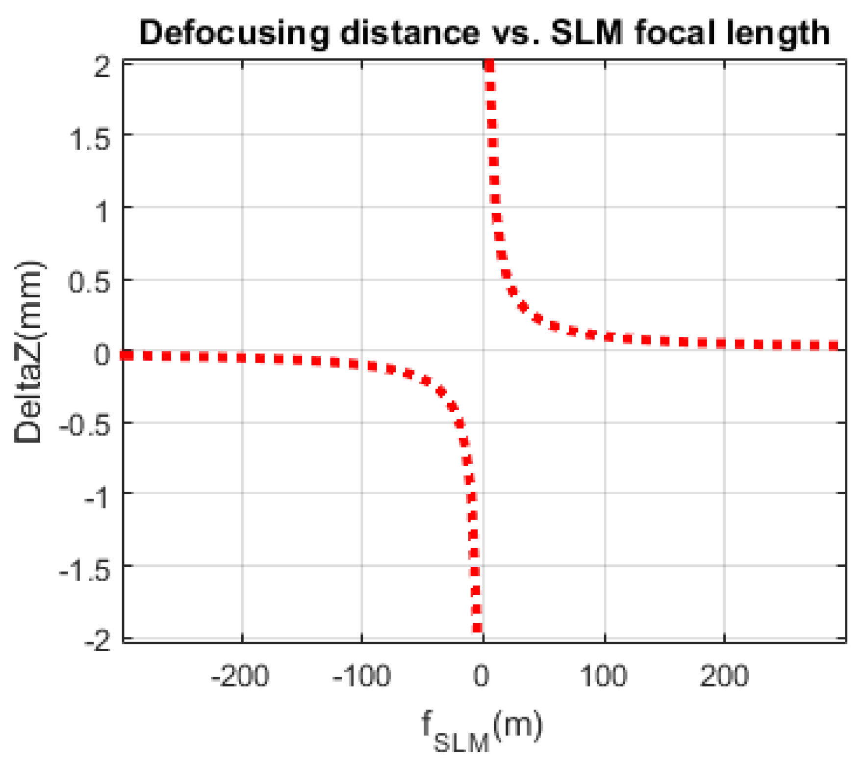
For the two optical systems to be equivalent, the phase term of Equation (8) and that of Equation (10) should be the same. Hence, we can easily derive a relation between the translation distance $∆z$ of the CCD in a traditional TIE system and the equivalent focal length $f_{SLM}$ of the quadratic phase pattern that should be displayed on the SLM. This relation can be written as

$${w_{SLM}\left(x,y\right)|}_{CCD}⟺{w\left(x,y,∆z\right)|}_{\begin{array}{c}∆z\\ from CCD\end{array}} ,\mathrm{if} ∆z= \frac{f^2}{f_{SLM}}.$$

(11)

Figure 3 shows the hyperbolic relation between the focal length $f_{SLM}$ of the quadratic phase pattern displayed on the SLM and the defocusing distance $∆z$ as shown by Equation (11) [33]. Since, the quadratic phase pattern displayed on the SLM can be modified much faster than the translation of the CCD camera, the new system can be used to reconstruct phase images of dynamical events. For the one-shot configuration shown in Figure 2a half of the CCD will hold the diffraction pattern from the mirror and the second half holds the diffraction pattern due to the quadratic pattern displayed on the SLM. For the two-shot configuration shown in Figure 2b two sequential recordings are needed, one when a positive quadratic pattern is displayed on the SLM corresponding to the over focused diffraction pattern $I_{OF}\left(x,y\right)$ and another when a negative symmetric quadratic pattern is displayed on the SLM corresponding to the under-focused diffraction pattern $I_{UF}\left(x,y\right).$

3. Tomographic Reconstruction Algorithm

The main purpose of this work is to obtain a fast and full field of view tomographic reconstruction of weakly scattering phase objects. To this end, a custom fabricated rotating stage assembly driven by a stepper motor that is controlled by Arduino microcontroller. At each angle of rotation of the stepper motor, two diffraction patterns ($I_{OF}\left(x,y\right)$ and $I_{UF}\left(x,y\right)$) are captured by the CCD camera either sequentially or at the same time depending on which setup is used in Figure 2.

Computing the 3-D refractive index (RI) of a sample from the multiple 2-D scattering fields, is an ill-posed inverse problem, which cannot be directly solved. Under the assumption of the weak scattering approximation, the inverse problem can be solved after linearizing the Helmholtz equation leading to either the Born approximation (optical delay of the sample ∆ψ < π/2) or the Rytov approximation $\left({\left(\overrightarrow{\nabla }\phi /k_0\right)}^2\ll ∆n\right)$ where $\overrightarrow{\nabla }\phi$ is the gradient of the phase and $∆n$ is the difference in refractive index between the sample and the medium [33,34,35,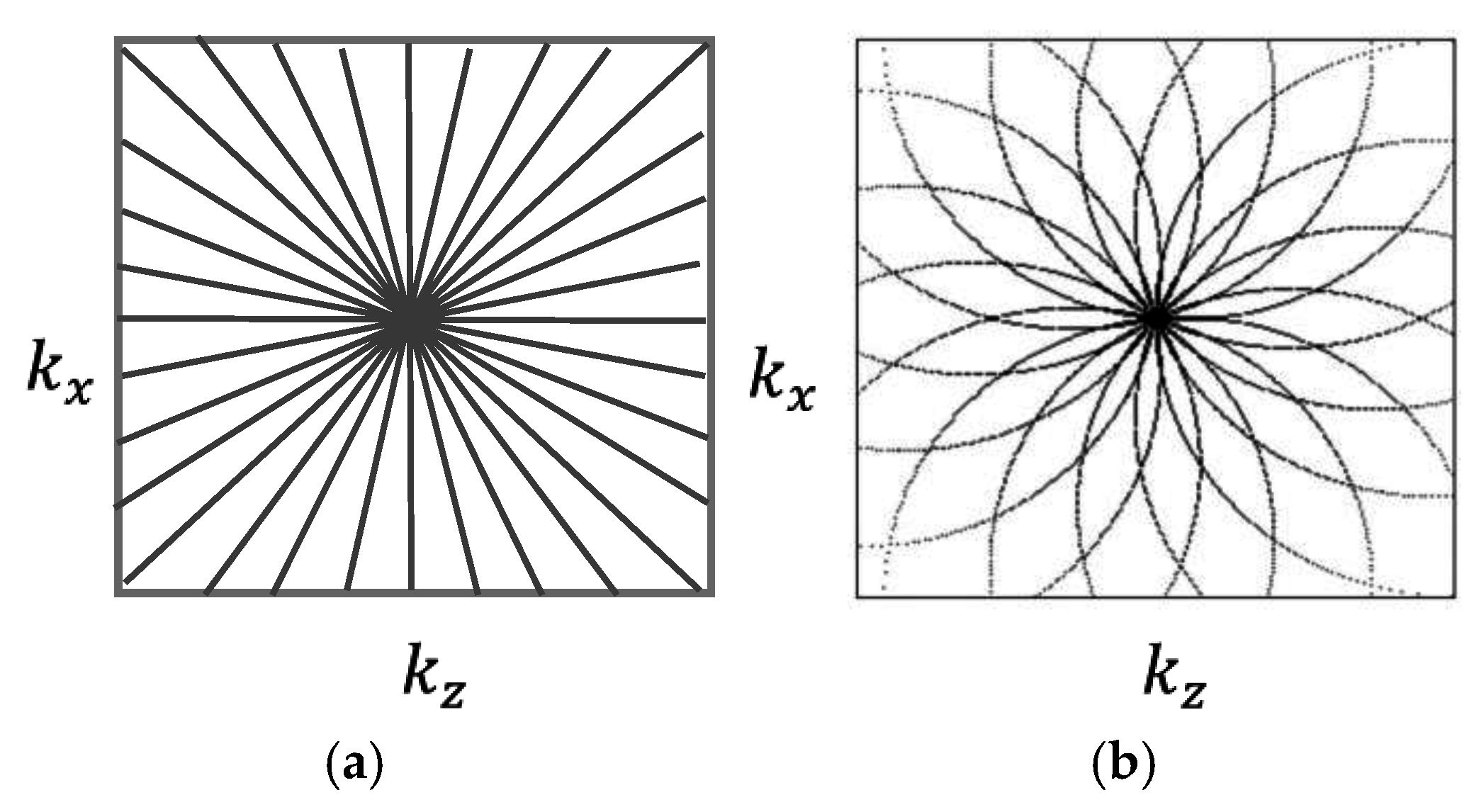36]. The phase objects tested in this study have low refractive index variation and the wavelength of illumination is much smaller than the size of the sample. Hence, the Fourier slice algorithm which neglects diffraction inside the sample and assumes that light propagates along straight lines with unchanged spatial frequency vectors, results in an accurate approximation of the 3D reconstruction (the wave propagation can be treated as projection). By applying the Fourier Slice theorem, the obtained spatial resolution is isotropic and no information is missing along the rotation axis. Figure 4 shows the difference in Fourier space representation between the projection (a) and the diffraction optical tomography (b). In this paper we will only use the projection approach shown in Figure 4a.

The reconstruction algorithm using the Fourier slice theorem works as follows: (a) Form the 3D projection matrix of the reconstructed phases using the TIE technique according to Equation (5) from P different projection angles ${\theta }_j=\left[0:\frac{j\pi }{P}:\pi \right], j=1,2,\dots ,P$; (b) Calculate the inverse radon transform (IRT) of the 3D projection matrix by computing the 2D IRT of each slice using the Fourier Slice theorem which states that the Fourier transform (FT) of a projection is a slice of the 2D FT of the region from which the projection was obtained [27,28,37]. The IRT is calculated according to the following equation:

$$G\left(\omega ,\theta \right)={{\displaystyle \int }}_{-\infty }^{+\infty }g\left(\rho ,\theta \right)e^{-j\omega \rho }d\rho ={F\left(k_x,k_y\right)|}_{\begin{array}{c}{k}_x=\omega cos\theta \\ k_y=\omega sin\theta \end{array}}=F\left(\omega cos\theta ,\omega sin\theta \right)$$

(12)

where $\rho =xcos\theta +ysin\theta ,$ $F\left(k_x,k_y\right)$ = ${\mathfrak{F}}_{2D}\left\{f\left(x,y\right)\right\},$ and

$$ℛ\left\{f\left(x,y\right)\right\}=g\left(\rho ,\theta \right)= {{\displaystyle \iint }}_{-\infty }^{+\infty }f\left(x,y\right)\delta \left(xcos\theta +ysin\theta -\rho \right)dxdy$$

(13)

is the Radon transform of $f\left(x,y\right)$ defined as [27]:

$$f\left(x,y\right)={\mathfrak{F}}_{2D}^{-1}\left\{G\left(\omega ,\theta \right)\right\}={{\displaystyle \int }}_0^{\pi }{{\displaystyle \int }}_{-\infty }^{+\infty }|\omega |G\left(\omega ,\theta \right)e^{j2\pi \omega �}d\omega d\theta .$$

(14)

Equations (12)–(14) suggest that the output of the IRT are slices $f\left(x,y\right)$ of the 3D reconstructed tomogram $f\left(x,y,z\right)$ of the original phase object and each of the $g\left(\rho ,\theta \right)$ images is a 2D phase retrieved using TIE at different projection angles. (c) Apply morphological post-processing techniques to obtain the final 3D shape of the object.

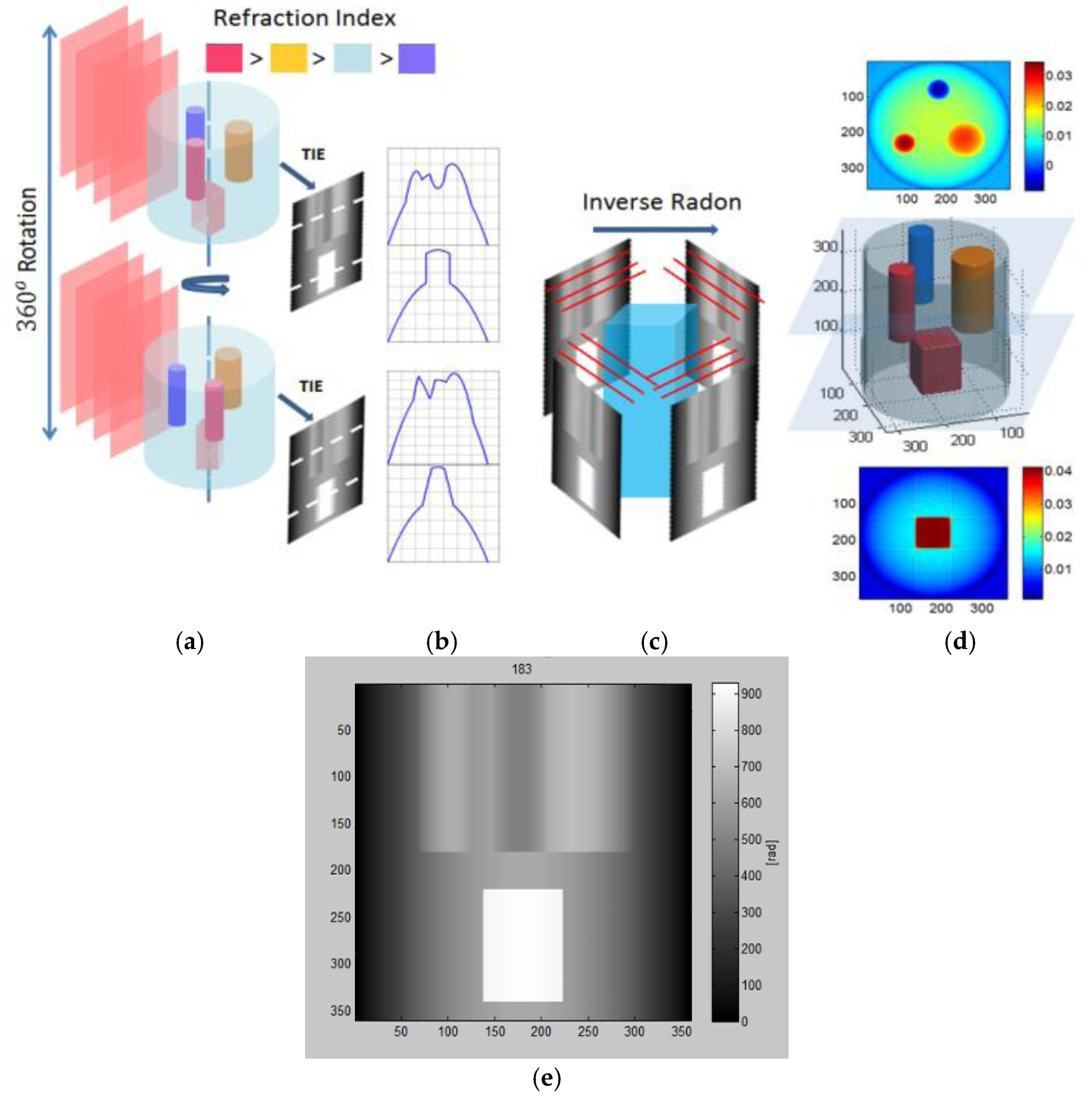
Consider a simulation example where TIE can be combined with the Fourier Slice theorem technique. In this example, three small cylinders and one cubic structure with indices of refractions (n_red, n_orange, n_violet) embedded inside a larger cylinder with index of refraction (n_blue). Phase projections with 1 degree angular spacing were created similar to those obtained experimentally by TIE. Figure 5a shows two different angular positions of the TIE simulated retrieved phases. Figure 5b shows 1D phase profile for each perspective. Figure 5c shows the application of IRT using slices from the TIE simulated retrieved phases. Figure 5d shows the 3D reconstruction of internal volume along with two horizontal slices of the structure. Figure 5e shows a screen capture of a 2D side view of the supplementary video. Hence, combining TIE with the IRT enables us to visualize the object’s internal structure. Note that for highly diffractive objects not immersed in matching liquid, optical diffraction tomography (ODT) should be used.

4. Experimental Results Using the SLM Based TIE 4f Setup

Consider the experimental 4f TIE setup in Figure 2. First, a Gaussian illumination beam passes through a three-axis spatial filter (Model 900) with pinhole 25 µm. The beam is then collimated by a lens resulting in a plane wave before illuminating the object. Two lenses L₁ and L₂ (focal length f = f₁ = f₂ = 100 mm) are used in a 4f configuration to image the object on the CCD camera. The monochrome CCD camera (Lumenera’s Lu100M series) has 1280 × 1024 pixels, with 5.2 µm pixel size, and with capturing speed of 15 fps. A positive or negative quadratic phase pattern is displayed on the phase only SLM (Holoeye Pluto) providing a lens effect which mimics the translation of the CCD as shown in Equation (11). Two experiments will be considered in this study.

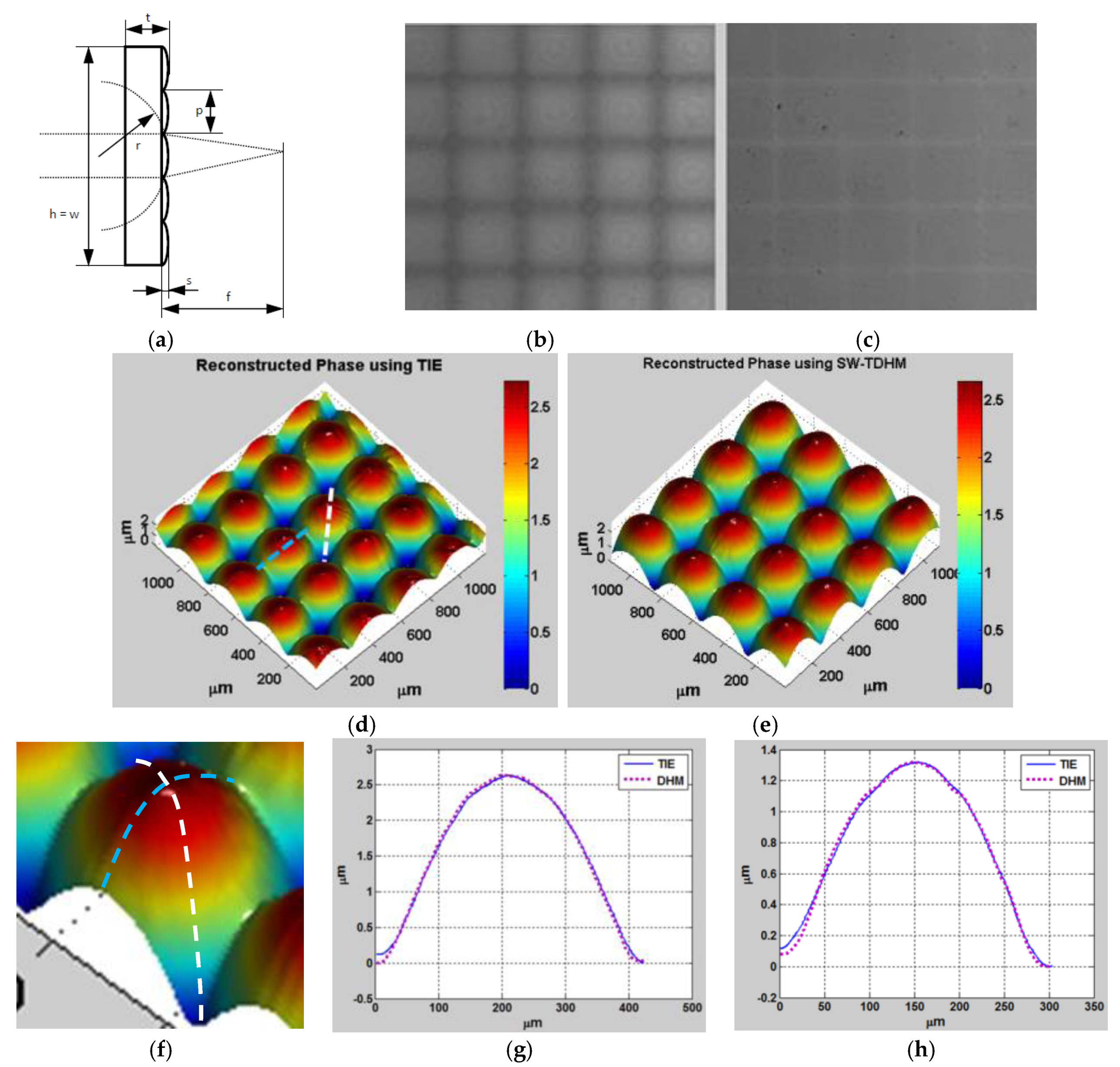
In the first experiment, a 625 nm partially coherent LED is used to mitigate speckle noise. The object used in this experiment is a plano-convex parabolic micro-lens array from Thorlabs as shown in Figure 6a.

Figure 6b,c show a single-shot intensity distribution from the mirror and the SLM, respectively. Figure 6d shows the 3D phase profile obtained using TIE. For validation, Figure 6e shows the 3D unwrapped reconstructed phase profile using digital holographic microscopy (DHM) and after automatic aberration cancellation using Zernike polynomials. Figure 6f shows a zoomed-in area of the lens array showing the profile locations under study. Comparison between the TIE and DHM techniques along the dashed white line and the dashed blue line are shown in Figure 6g,h, respectively. Notice that no phase unwrapping is needed in the case of TIE, which is one of the main advantages of this technique as unwrapping error is eliminated. Note that the sample shows that the profile height along the blue line is $s_1=1.3\mathsf{\mu }\mathrm{m}$ and the profile height along the white diagonal line is $s_2=2.6 \mathsf{\mu }\mathrm{m}.$

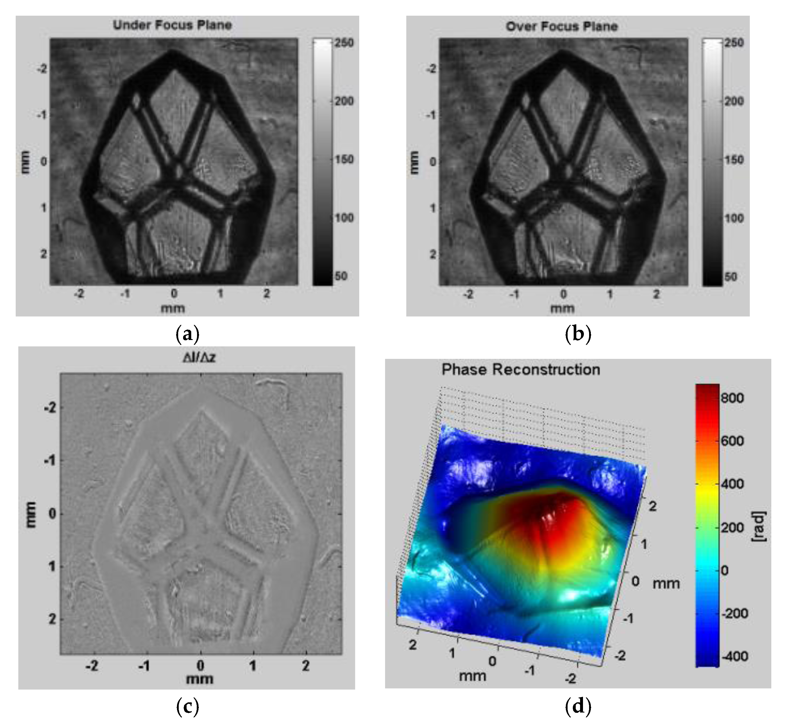
As a second experiment, a coherent HeNe laser source is used to illuminate a glass diamond-shaped bead according to the configuration shown in Figure 2b. After displaying the appropriate quadratic phase patterns on the SLM, Figure 7a,b show the two intensity distributions ($I_{OF}\left(x,y\right)$ and $I_{UF}\left(x,y\right)$) of the object illuminated by a plane wave captured at the CCD as if ∆z = $\pm$0.5 mm, respectively. Figure 7c shows the difference between these two intensity distributions, and Figure 7d shows the reconstructed phase profile of the object. Note that the glass bead is a complex shape to reconstruct than the smooth microlens array because of the rough edges that contain higher frequencies and can scatter more light before it is captured by the lenses. The glass bead was also immersed in matching oil with a refractive index of 1.515, close to the refractive index of the object, which is 1.541, to avoid light scattering as much as possible. In this experiment, 10 projections were enough to get a decent result. The more projections recorded, the better the 3D reconstruction result will be, at the expense of more computation time. Background cancelation and padding were also used in pre-processing to get better results in phase. Note that the dark areas still have some low intensity values and thus phase can still be recovered in these regions.

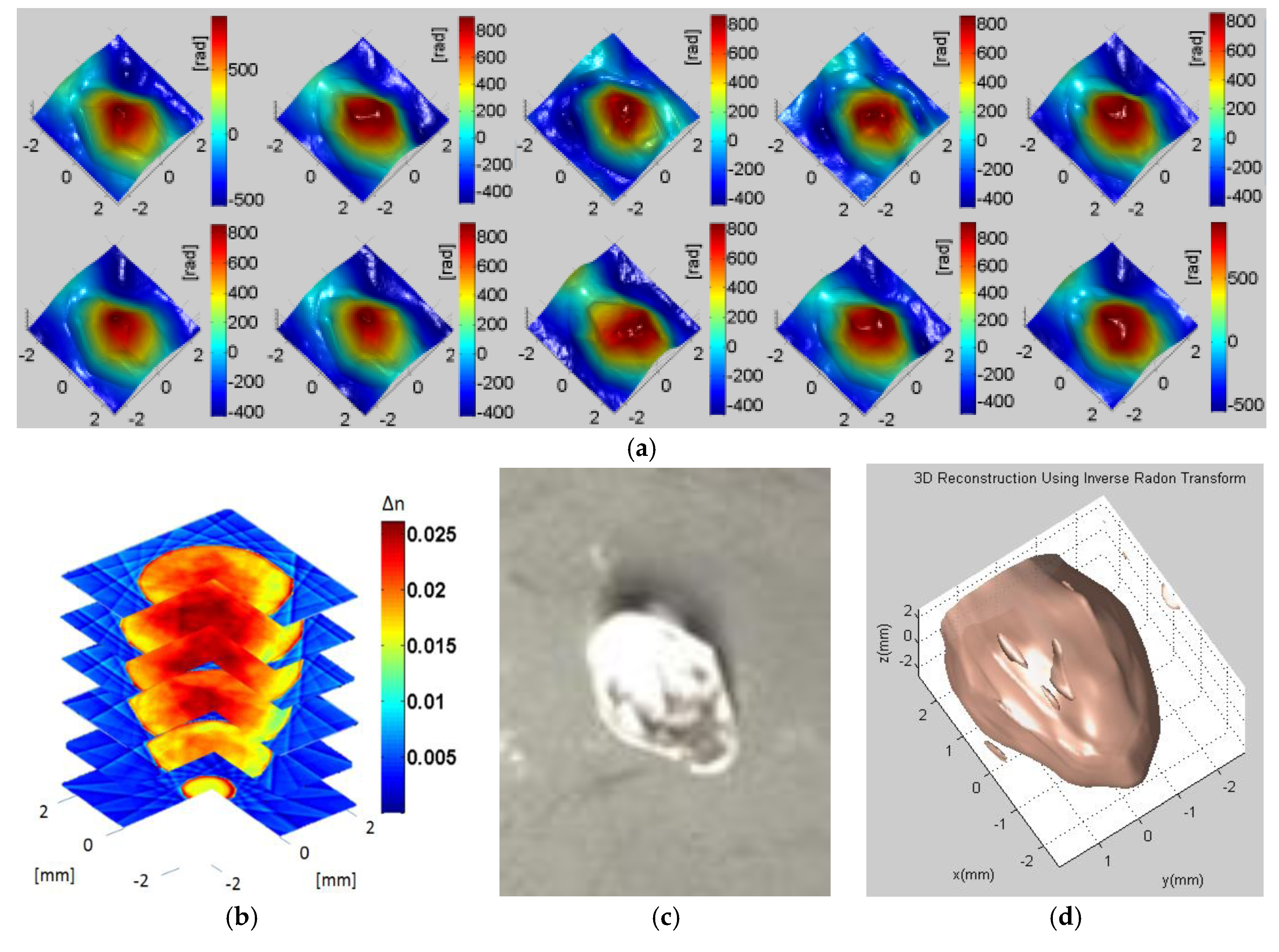
Figure 8a shows the reconstructed phases at 10 different projections with 36° spacing between consecutive projections. Figure 8b shows the slices of the 3D tomographically reconstructed diamond shaped bead using the Fourier Slice theorem where small refractive index variation is clearly visible. Figure 8c shows a photograph of the diamond-shaped bead, and Figure 8d shows the reconstructed outer surface of the object.

As a third experiment, we use the TIE setup shown in Figure 2 to visualize dried pine pollen cells from Amscope placed between microscope slides. Figure 9a–c show the intensity distributions of a dried pollen cell at ∆z = 1, 0, −1 mm. Figure 9d shows the derivative of intensity over the propagation direction. Figure 9e shows the 3D height distribution converted from phase [7], and Figure 9f is an image of pine pollen seen under a bright field microscope. We should note that since the pollen cells are dried the wings have smaller phase than the cell body.

As a fourth experiment, we used the TIE setup shown in Figure 2 to tomographically visualize cancer cells placed in a glass micropipette (Duran^® Borosilicate glass) which was immersed in a matching index oil with an index of refraction of 1.47. For Figure 10, the triple-negative cancer cells from the highly invasive MDA-MB-231 breast cancer cell line were cultured on glass bottom Petri dishes and fed with DMEM supplemented with 10% FBS. Imaging was performed after 24 h incubated at 37 °C, in a 5% CO₂ humidified incubator. A 10 nm HEPES buffer was used during imaging to avoid pH rising. 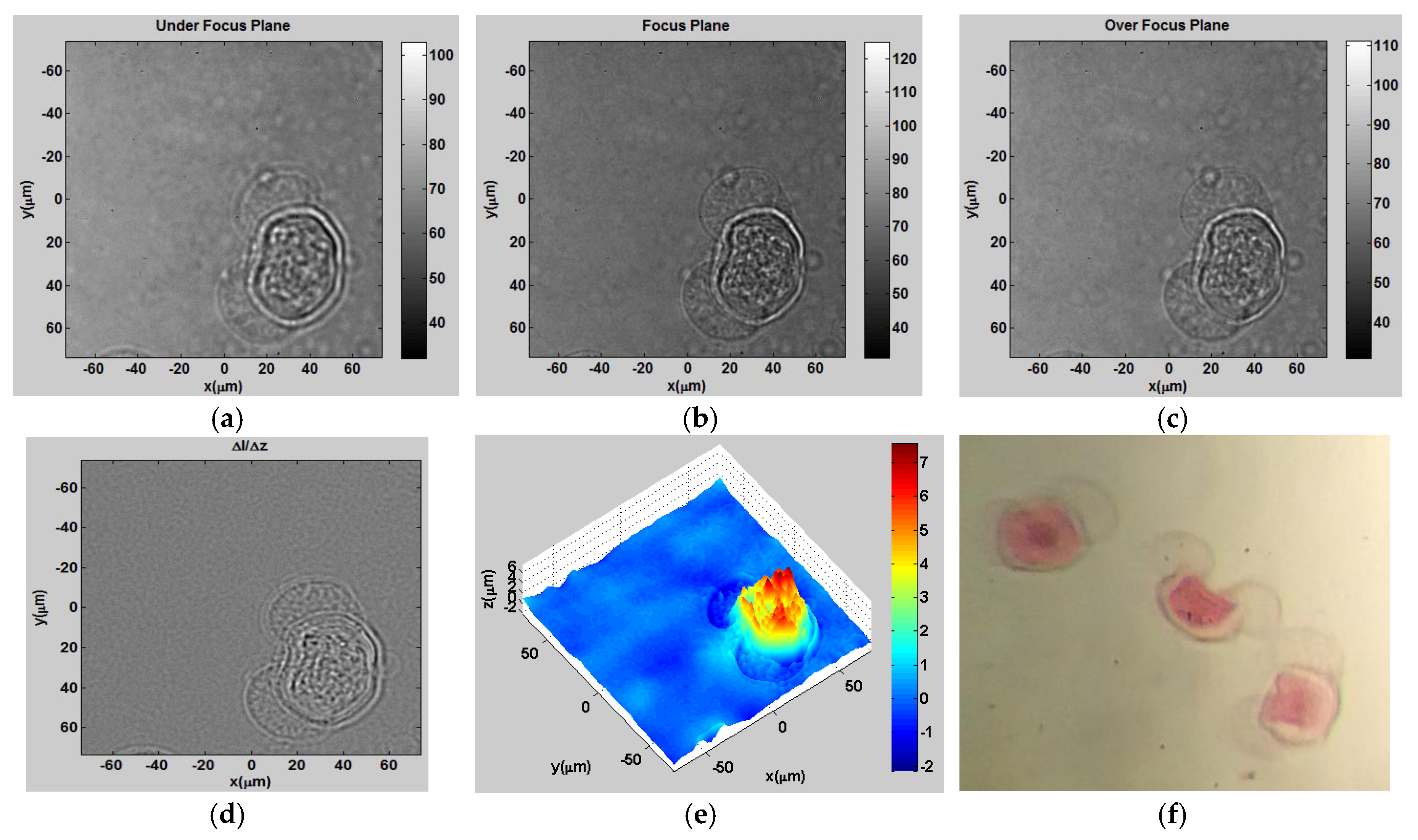Figure 10a–c show the intensity distributions of cancer cells at the underfocused, focused, and over-focused planes, respectively. Figure 10d shows the derivative of the intensity over the propagation direction z, and Figure 10e shows the 3D height distribution using TIE.

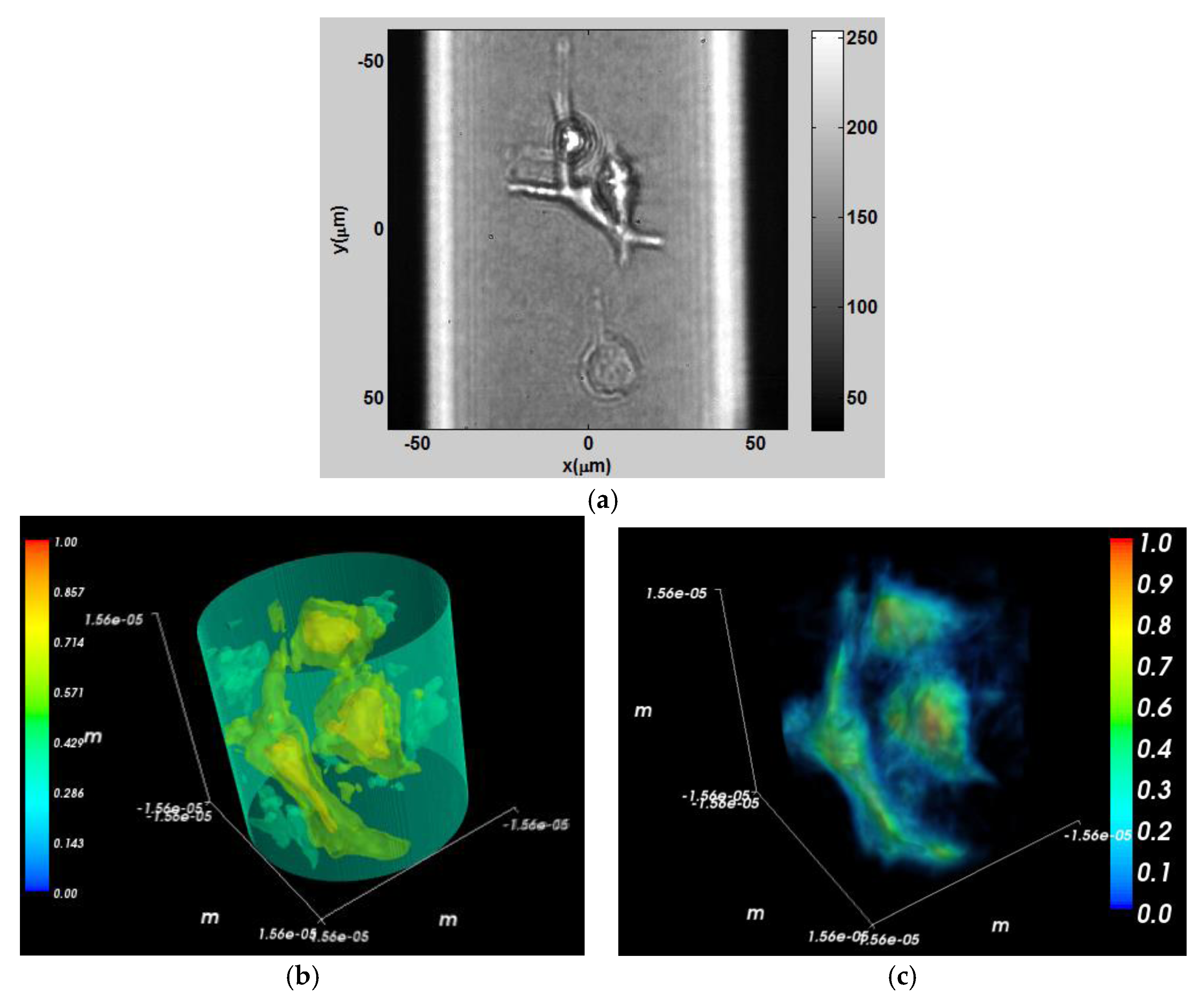
As a fifth experiment, the same line of cancer cells were mixed with collagen I with 4 mg/mL concentration to achieve 3D culturing. Cell-collagen mixture was quickly pumped to micropipette tips (200 µm in diameter and 1 μL in volume) and incubated overnight at 37 °C and 5% CO₂ humidified incubator for tomographic measurement. The micropipette is mounted under a rotator that acted like a spinner [38]. Thirty-six different projections with 10° angular spacing between consecutive projections were reconstructed with similar rotation configuration as in the diamond object experiment. Python software was used for 3D rendering which gives better visualization than MATLAB^®. Figure 11a shows the intensity distribution of a group of three cells placed in the micropipette. Figure 11b shows the 3D contour visualization of the refractive index. In Figure 11b the scale is normalized between the refractive index of the collagen mixture and the cancer cells (1.35–1.38). Figure 11c shows a 3D refractive index visualization with transparent 3D rendering. In Figure 11c the data was normalized to provide a better view of the internal structure of the cells.

5. Discussion of the Hardware and Software Used for the SLM-Based TIE System

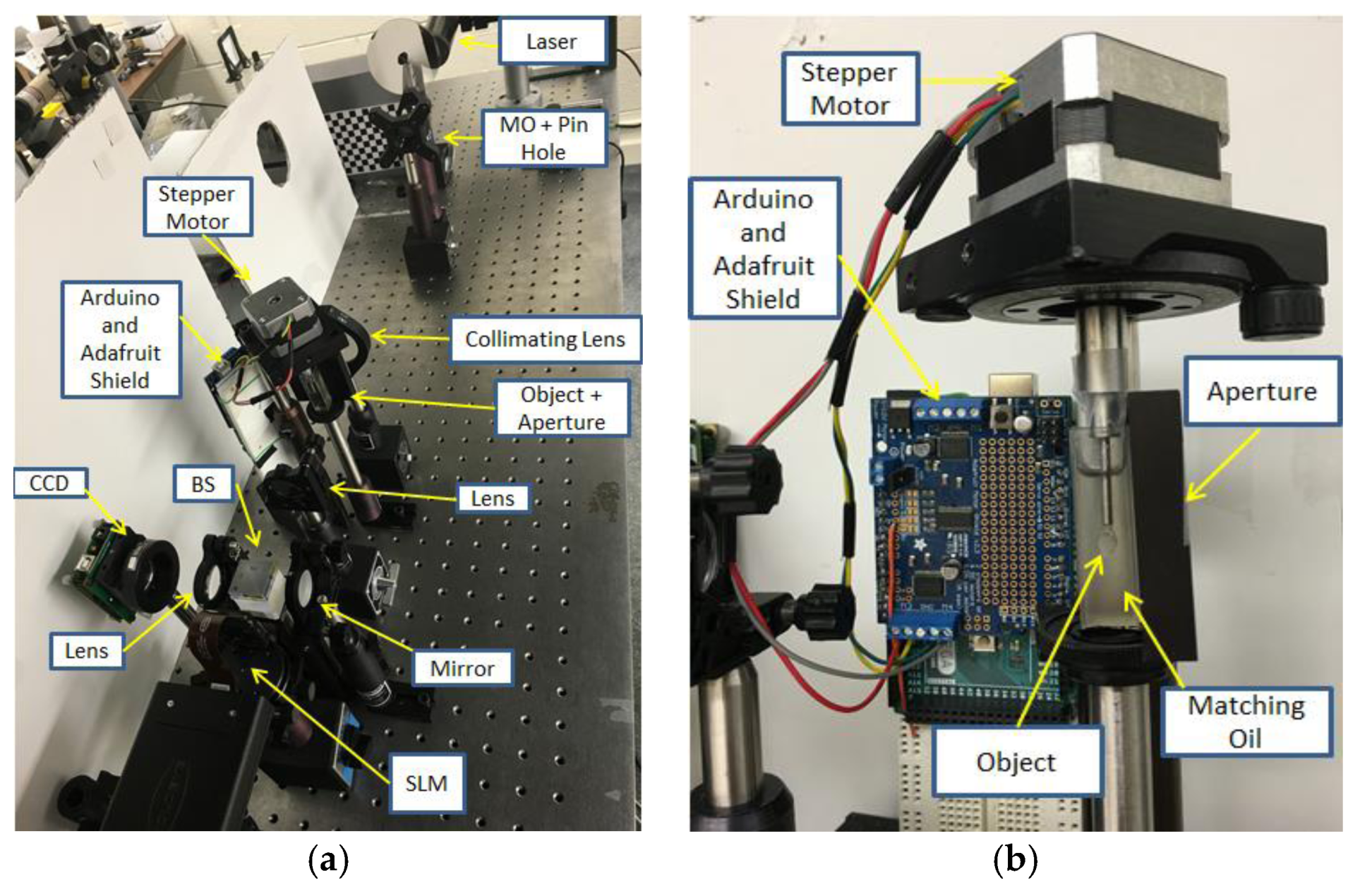
Figure 12a shows the laboratory optical setup of the SLM-based TIE system and Figure 12b shows the Arduino-controlled rotating stage assembly. The TIE and the 3D tomographic reconstruction process was implemented on an Alienware 15 laptop using MATLAB^® 2014a with a NVIDIA GeForce GTX 970M graphics card and 8 GB RAM DDR4.

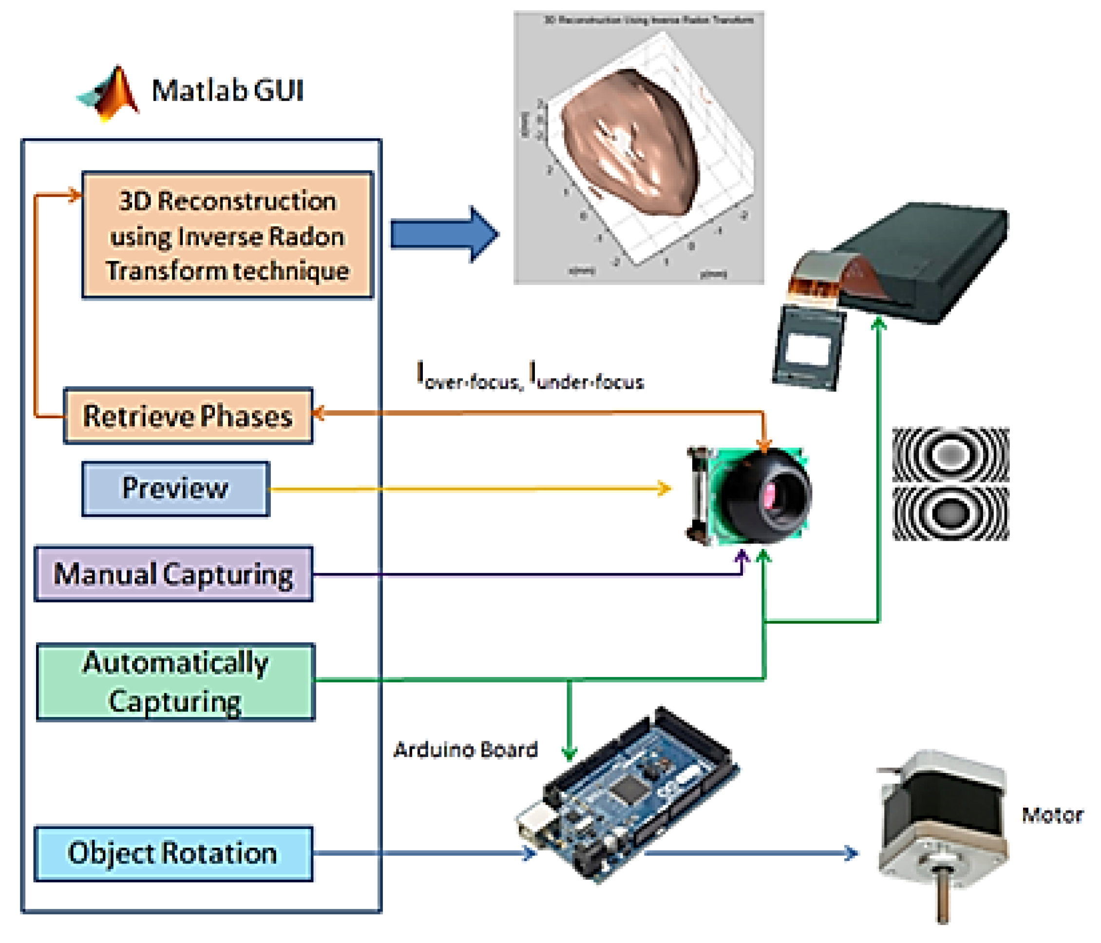
Figure 13 shows the block diagram of the recording and reconstruction process which contains the GUI, the Arduino microcontroller, the CCD, the SLM, and the stepper motor. Also, this figure shows how all the parts of the system are interconnected.

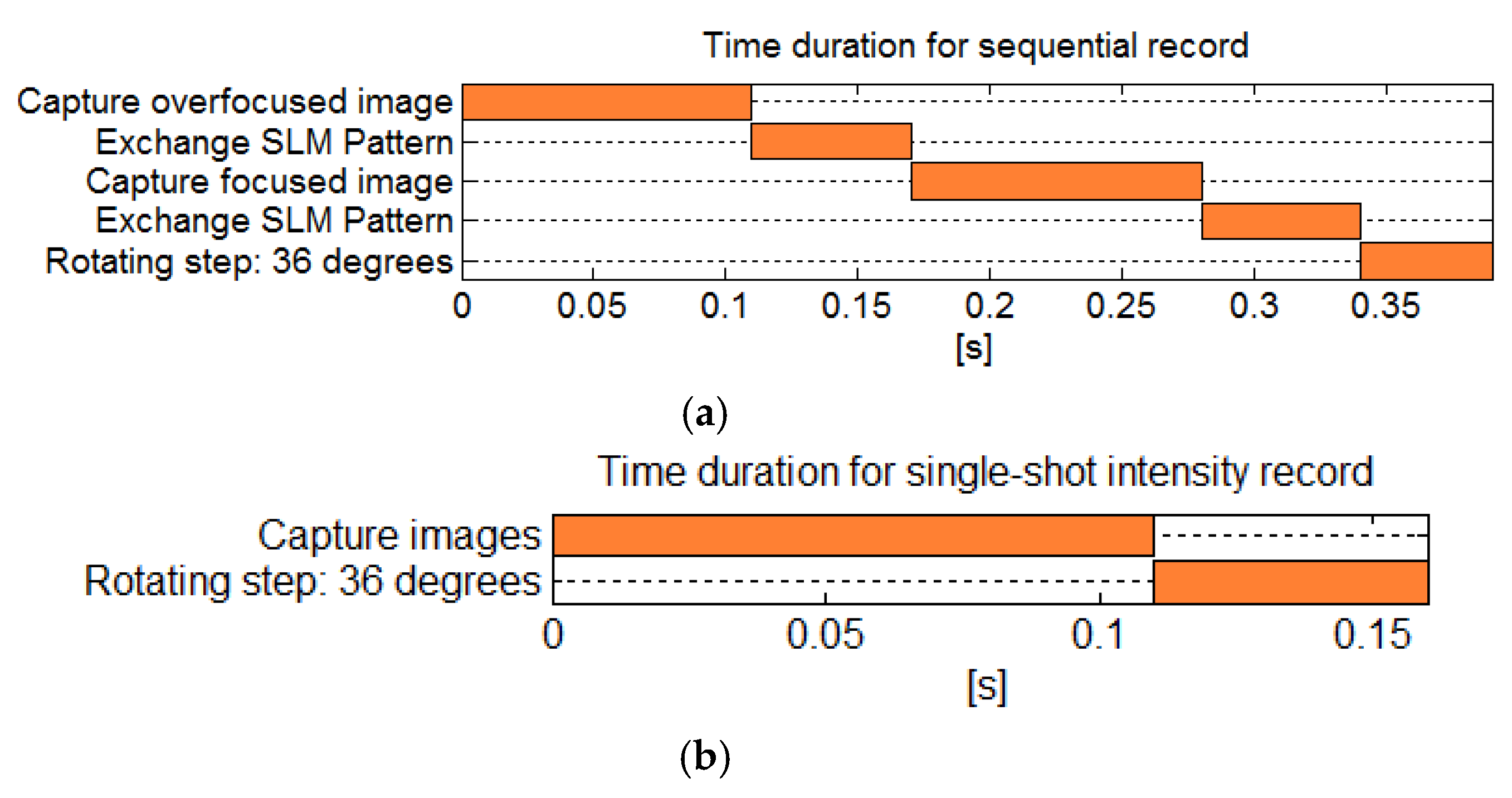
In the sequential recording setup, the total recording time for capturing two intensity images is 0.22 s, exchanging SLM’s pattern two times takes 0.12 s, and the rotation using the stepper motor takes 0.05 s per step (Figure 14a). Hence, it takes 3.9 s to record the 360° tomogram. In the single-shot setup, the camera captures both intensity images at the same time and it does not require changing the SLM’s patterns, and hence it takes 1.6 s to record a 360° tomogram (Figure 14b).

Hence, the total recording time depends on the speed of the camera and motor. The total time to record a tomogram in single-shot setup with ten perspectives is 1.6 s. In our laboratory, we have a low-price stepper motor and camera. Faster cameras and motors will be able to record live tomograms. After recording all intensities, phases are reconstructed off-line based on TIE and the Fourier Slice theorem techniques. In the MATLAB^®-developed code for this paper, the time duration for the reconstruction process is 14.6 s. An additional step of pixel intensity matching is necessary in the single-shot setup. This can be done by tracking the position of 4 corners of rectangular aperture before the object. Note that when using GPUs and C++, a faster reconstruction time can be achieved [39].

6. Conclusions

In this paper, we developed a TIE optical system for phase retrieval using a spatial light modulator with a rotating assembly to achieve full field of view 3D tomographic reconstruction. This SLM-based tomographic TIE optical setup can be used for 3D tomographic reconstruction of static as well as dynamic macroscopic and microscopic phase objects. Also, we have derived the theory behind the SLM based TIE methodology and proved by simulation and experimentation the validity of the 3D tomographic reconstruction using the Fourier slice theorem. Synchronization between the CCD, the SLM, and the rotating stage was employed using an Arduino microcontroller and a MALTAB^® based user friendly GUI that also performs the tomographic reconstruction process. In the future we are planning to use a faster motor and CCD camera and develop a 3D reconstruction algorithm using GPU-based reconfigurable hardware to achieve better reconstruction times while maintaining higher-resolution 3D tomograms.