Detection and Classification of Land Crude Oil Spills Using Color Segmentation and Texture Analysis

Ejofodomi, O’tega; Ofualagba, Godswill

doi:10.3390/jimaging3040047

Open AccessArticle

Detection and Classification of Land Crude Oil Spills Using Color Segmentation and Texture Analysis

by

O’tega Ejofodomi

^* and

Godswill Ofualagba

Racett Canada, Inc., 404 St. George Street, Moncton, NB E1C 1X0, Canada

^*

Author to whom correspondence should be addressed.

J. Imaging 2017, 3(4), 47; https://doi.org/10.3390/jimaging3040047

Submission received: 18 August 2017 / Revised: 9 September 2017 / Accepted: 13 September 2017 / Published: 19 October 2017

Download

Browse Figures

Versions Notes

Abstract

:

Crude oil spills have negative consequences on the economy, environment, health and society in which they occur, and the severity of the consequences depends on how quickly these spills are detected once they begin. Several methods have been employed for spill detection, including real time remote surveillance by flying aircrafts with surveillance teams. Other methods employ various sensors, including visible sensors. This paper presents an algorithm to automatically detect the presence of crude oil spills in images acquired using visible light sensors. Images of crude oil spills used in the development of the algorithm were obtained from the Shell Petroleum Development Company (SPDC) Nigeria website The major steps of the detection algorithm are image preprocessing, crude oil color segmentation, sky elimination segmentation, Region of Interest (ROI) extraction, ROI texture feature extraction, and ROI texture feature analysis and classification. The algorithm was developed using 25 sample images containing crude oil spills and demonstrated a sensitivity of 92% and an FPI of 1.43. The algorithm was further tested on a set of 56 case images and demonstrated a sensitivity of 82% and an FPI of 0.66. This algorithm can be incorporated into spill detection systems that utilize visible sensors for early detection of crude oil spills.

Keywords:

crude oil spills; crude oil spill detection; image segmentation; texture feature extraction; automated spill detection

1. Introduction

Crude oil spills have severe negative effects on the environment, health, society and economy of the nation in which they occur, and this has been documented extensively in scientific literature [1,2,3,4,5,6,7,8,9,10]. In the United States, 217 spill incidents were reported and 43,662 barrels (6,942,258 L) spilled in 2007 [11]. In Canada, 133 spill incidents were reported to the Transportation Safety Board of Canada for federally regulated pipelines in 2014 [12]. The Niger Delta region of Nigeria is considered to be one of the most severely petroleum-damaged ecosystems in the world [8]. The Department of Petroleum Resources of Nigeria reported a total of 871 spill incidents and 15,552.18 bbl (2,472,796.6 L) of oil released into the environment in 2012 [13].

When a spill occurs in water or offshore, contact and ingestion of spilled oil leads to contaminants in tissues, DNA damage, impacts to immune functioning, cardiac dysfunction, mass mortality of eggs and larvae, and the loss of buoyancy and insulation for birds [14,15,16,17,18,19,20,21]. When the spill occurs on land, it prevents soil aeration, affects soil temperature, structure, fertility, pH, and results in the destruction soil micro-organisms and agricultural crops [22,23]. Other effects include contamination of ground water, loss of biodiversity in breeding grounds, vegetation hazards, loss of portable and industrial water resources, reduction in fishing and farming activity, poverty and rural underdevelopment [24].

Direct or indirect contact with crude oil can result in short-term symptoms such as headaches, fatigue and lethargy, eye, nose and throat irritation, loss of concentration and co-ordination, dizziness, nervousness, insomnia, nausea, vomiting, visual disorders, drowsiness, depression, heightened anxiety, skin rashes and sores, respiratory disorders like shortness of breath, and exacerbation of asthma [25,26]. Long-term effects on humans include DNA degradation, cancers, birth and reproductive defects, irreversible neurological and endocrine damage, and impaired cellular immunity [1,19,21,27,28].

Loss of crude oil due to spills results in a decrease in a nation’s revenue. In 2014, 1,008,805 bbl (160,400,000 L) of crude oil were lost from Nigeria’s pipelines, resulting in a loss of N14,846,710,000 [29]. Crude oil spills also demand exorbitant financial resources to remediate or clean up the damaged environment. For example, the 1989 Exxon Valdez spill cost Exxon $4.8 billion for remediation, compensatory payments, settlements and fines [30].

Several methods have been employed for spill detection, including real-time remote surveillance by flying aircrafts with surveillance teams. Other methods employ various sensors such as visible sensors, infrared sensors, ultraviolet sensors, radar sensors, and laser fluorosensors [31,32]. Most of these methods generate some type of image that is used in detecting and assessing the size of the spill. The image analysis performed on the acquired images usually involves segmentation, horizon detection, and classification. Segmentation is performed to identify and extract the object of interest in the image [33,34]. In particular, color segmentation has proven to be extremely effective in distinguishing objects [35]. A color image provides three times more data than a grayscale image, since it can be represented by the three monochrome components defined by RGB, HSV, XYZ or CIELUV color spaces. RGB is widely used for its simplicity [35]. Some common methods of color segmentation include histogram thresholding and edge detection [36,37]. Effective horizon detection is required in order to identify sea-sky, soil-sky and forest-sky boundaries [38] and the algorithms that have been developed to do this are based on experiments carried out by authors in the published literature [38], and classification is performed after objects have been successfully identified in the image and it is crucial in determining the effectiveness of the algorithm [39].

There are several methods that have been employed in detecting oil spills in images, and they include the automatic statistical approach [40], neural network classification [41], wind history information [42], spill detection near offshore platforms [43], and probabilistic approach [44]. Feature extraction and spatial analysis also play a very important role in detection of oil spills in images [45,46].

The main systems to monitor sea-based oil pollution are the use of airplanes and satellites equipped with Synthetic Aperture Radar (SAR). SAR is an active microwave sensor, which captures two-dimensional images, and as such the spill detection algorithms developed so far are mainly focused on SAR images [39]. This paper presents an algorithm to detect the presence of crude oil spills automatically in images acquired using visible light sensors. To our knowledge, this represents one of the first spill detection algorithms developed specifically for images acquired with visible light sensors. Images of crude oil spills used in the development of the algorithm were obtained from the Shell Petroleum Development Company (SPDC) website [47]. The spill detection algorithm used in this paper is discussed in detail in the Materials and Methods section. The results obtained from the implementation of the algorithm on crude oil spill images derived from the SPDC website are presented in the Results section. Challenges encountered and possible options to improve the efficiency of the algorithm are expounded on in the Discussion and Conclusion section.

2. Materials and Methods

2.1. Materials

All crude oil spill images used in the development and testing of the algorithm proposed in this paper were obtained from the SPDC Nigeria website [47]. A total of 25 images were selected and used in the development of the spill detection algorithm. These images were classified as sample images. For each sample image, color and texture information of selected regions containing crude oil spills were extracted. The texture information utilized in characterizing crude oil spills were homogeneity, entropy and the power spectrum density of the selected region. The color and texture information obtained from the sample images were used to obtain optimal thresholding values for automated extraction of crude oil spills present in any given image. The algorithm was developed and tested using MATLABTM (The MathworksTM, Natick, MA, USA).

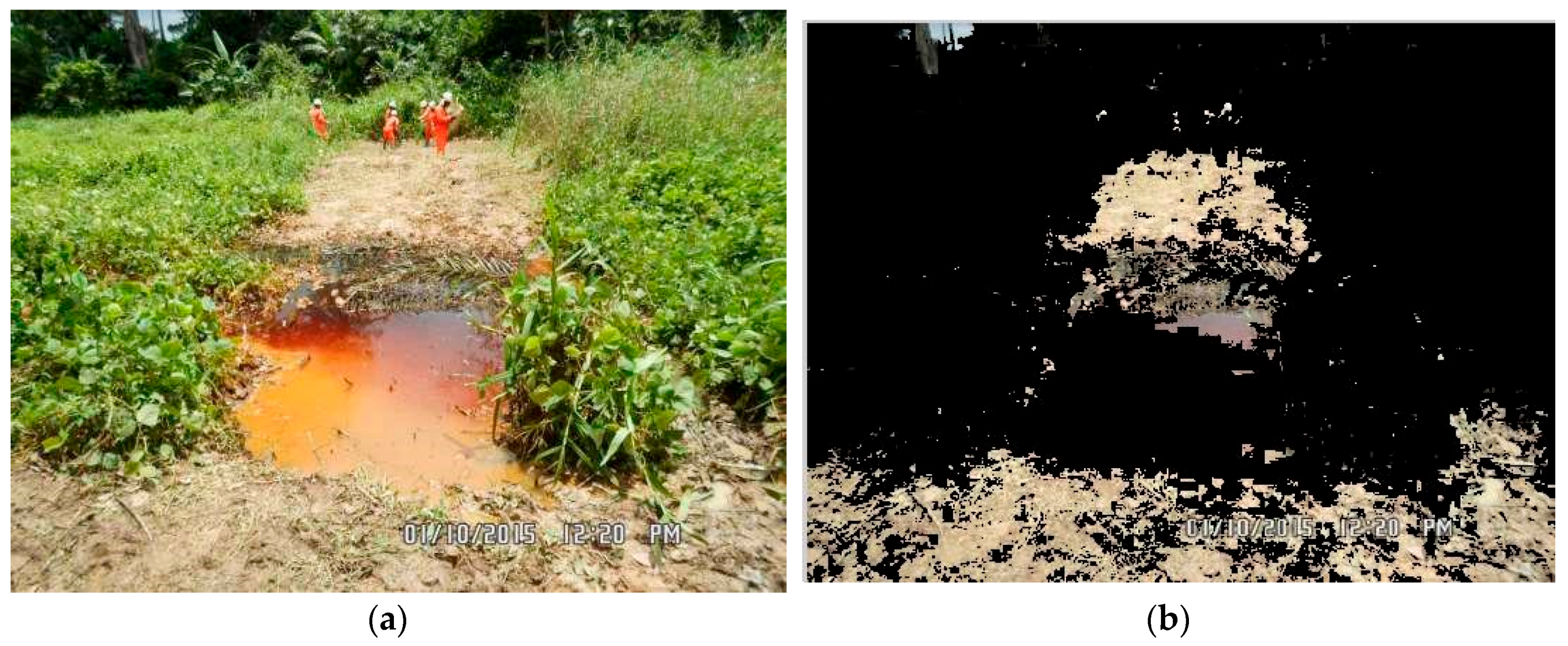
After the successful development of the spill detection algorithm, the algorithm was tested further on case images also drawn from the SPDC website. A total of 56 case images were utilized in testing the efficiency of the crude oil spill detection algorithm developed with the aid of the 25 sample images. The 56 case images contained crude oil spill with varying volumes, making it possible to test the ability of the algorithm to detect minute spills as well as large-volume spills. Figure 1a,b show sample images from the sample and case images respectively.

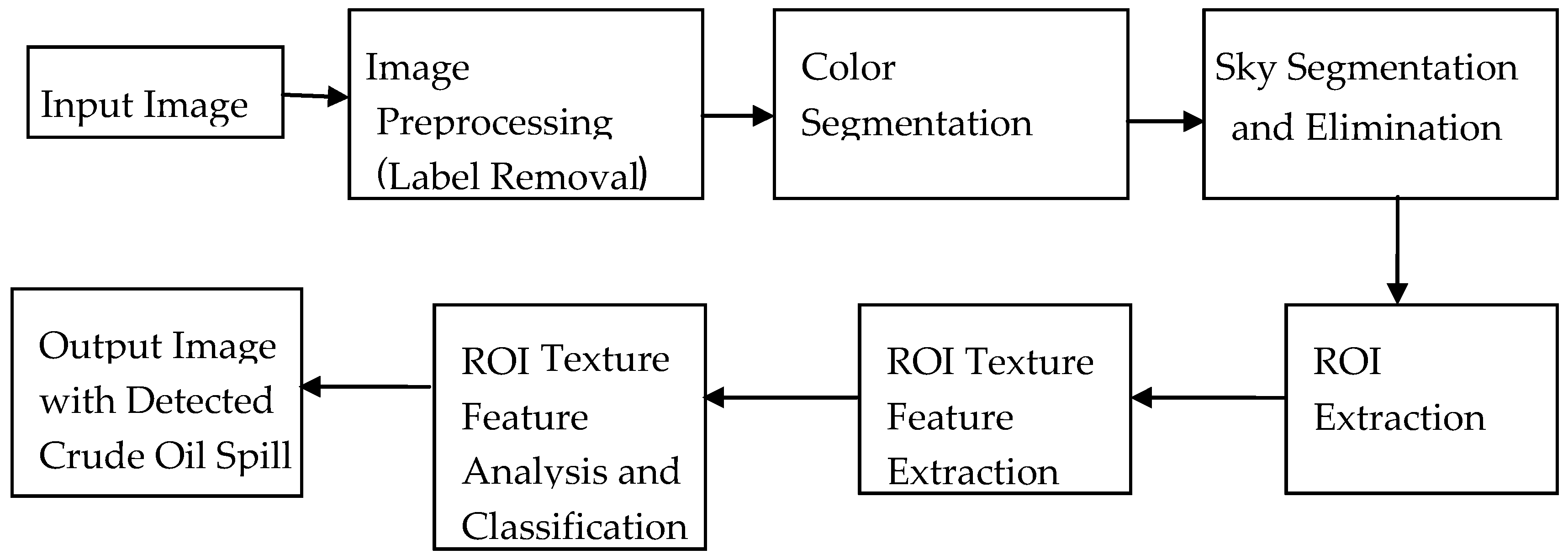
2.2. Methods

The crude oil spill detection algorithm developed using the sample images is depicted in Figure 2. It involves six major steps. These are image preprocessing, crude oil color segmentation, sky elimination segmentation, Region of Interest (ROI) extraction, ROI texture feature extraction, and ROI texture feature analysis and classification.

The algorithm to detect and extract crude oil spills from images was developed using the 25 sample images, using a step-wise procedure. For instance, the image preprocessing code to ensure the removal of the labels from the image was developed and tested on the 25 sample images. If the code failed to successfully remove the labels in any of the 25 images, the authors conducted further revisions and modifications to the code until the final image preprocessing code was able to successfully remove the labels in all of the 25 images. Once this was done, the final image preprocessing code was integrated into the spill detection algorithm. The same process was repeated for the remaining five major steps shown in Figure 2.

This step-wise procedure was necessary in order to ensure the final spill detection algorithm was optimized to ensure the highest possible sensitivity along with the minimum number of False Positives per Image (FPI). Once this was accomplished, the final spill detection algorithm was implemented on the 56 case images. These images were chosen at random from [35] to ensure an unbiased evaluation of the developed spill detection algorithm. The final algorithm can also be further tested on other image sets. The authors use the term “sample” to explain that those images were used to experimentally develop the spill detection algorithm and to refine and improve it until it demonstrated maximum sensitivity along with minimum FPI. Once that was accomplished the final algorithm was then tested on another set of images referred to as case images to verify and validate the algorithm’s efficiency.

2.2.1. Image Preprocessing

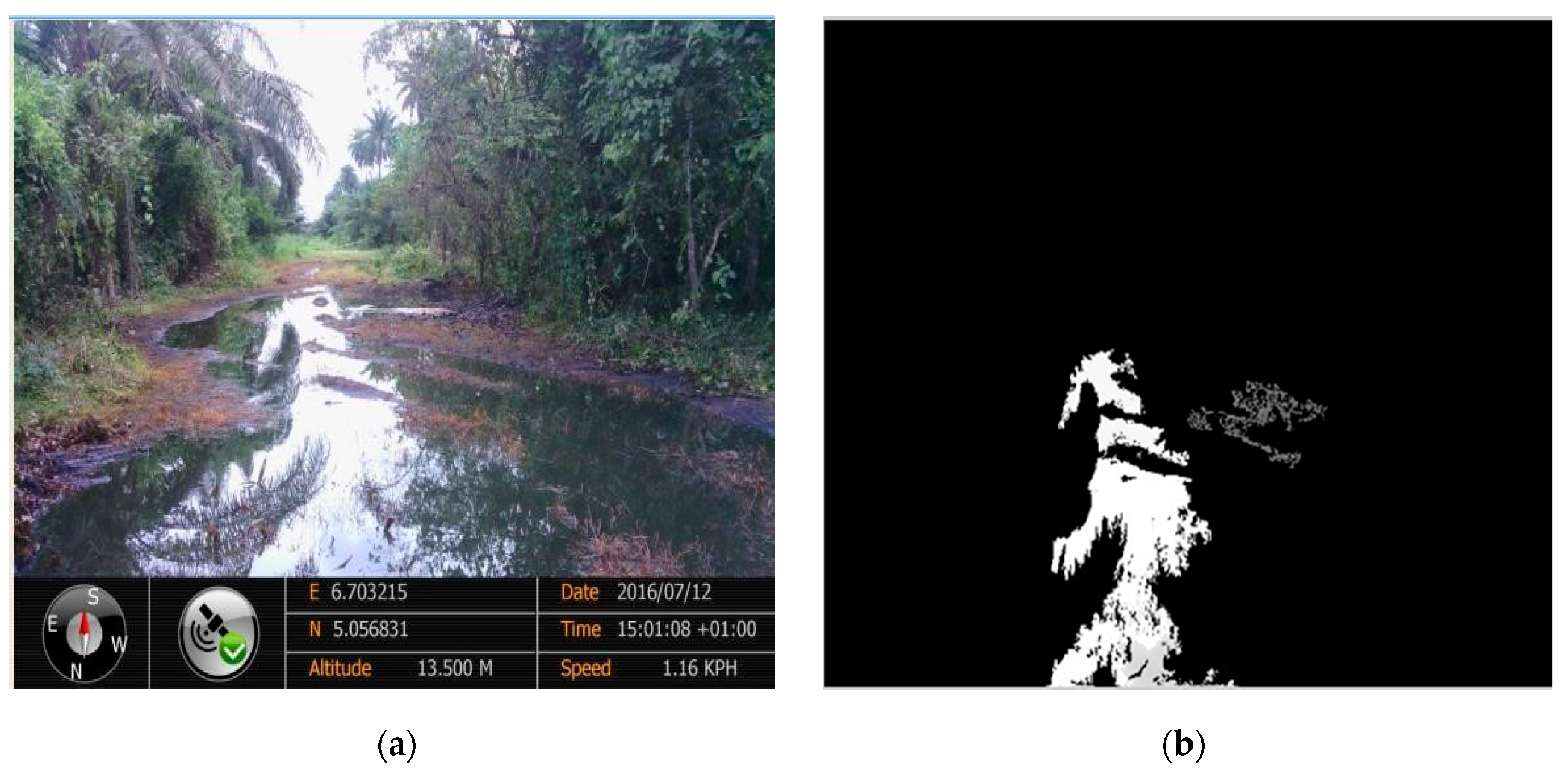
Some of the images obtained from the SPDC website contained labels at the bottom which affected the algorithm’s ability to accurately detect crude oil spills in the images. Figure 3a shows a case image with its label. The label typically contained Global Positioning System (GPS) location of the spill, as well as the date and time the image was acquired. To prevent these label pixels from interfering with the identification of the spill, they were removed during the preprocessing stage of the algorithm (see Figure 3b).

For the images obtained from [35], the labels were typically at the bottom of the images (see Figure 3a) and the size of the labels were dependent on the image height, h. For an input Image, InitialImage, the bottom rows containing the label pixels were removed using the following procedure shown Number 1 in the Appendix A.

As stated, the size of the label was dependent on the image height and this was taken into account in the algorithm. After label removal, the output image, PreprocessedImage was then passed on to the second stage of the spill detection algorithm. Other datasets may require no label removal if they have no labels, or the position of their labels may be in a different location in the image, at the top of the image, and the algorithm may need to be adjusted if that is the case. However, the presence of label in the images affects the sensitivity of spill detection algorithms so this is a very important step that should not be overlooked.

2.2.2. Color Segmentation

Most crude oil spill images contain at least three major regions when classified by color: sky, vegetation and land. In some of the images used in this paper, only one or two of these regions were present. The colors for each of these regions are distinct. The color of the sky ranged from white to blue, the vegetation was primarily green, and the color of the ground was brown. Each color has a distinctive range in the RGB color spectrum and this information was exploited in the development of the color segmentation portion of the spill detection algorithm. Color analysis performed on regions containing crude oil spills in the sample images was used in determining the range of colors exhibited by crude oil spills. This experimentally determined color of crude oil spills was found to be predominantly in the brown region. Therefore, color thresholding was performed on the preprocessed image to extract regions that possessed the same color attributes as the crude oil spills in the sample images. Figure 3c shows a color-segmented image of one of the case images used in this study. Note that the green vegetation has been eliminated from the color-segmented image. This portion of the algorithm extracts out of the vegetation in the image, leaving behind the sky and land pixels.

For an Input Image, PreprocessedImage, the vegetation in the image was removed using the following procedure shown in Number 2 of the Appendix A. The values for V_T1A, V_T1B, V_T2A, V_T2B, V_T3A, and V_T3B were determined experimentally during the development of the algorithm using the sample cases. Afterwards, the optimal value for each of those parameters was utilized in the final algorithm and also for testing the algorithm on the sample cases. If a pixel, p(i,j), had its, R, G, and B, values within the minimum and maximum threshold identifying vegetation, then it was a pixel containing vegetation and that pixel was eliminated by assigning it the RGB value for black (0,0,0). The output image VSegmentedImage, was then passed on to the next stage of the algorithm.

2.2.3. Sky Segmentation and Elimination

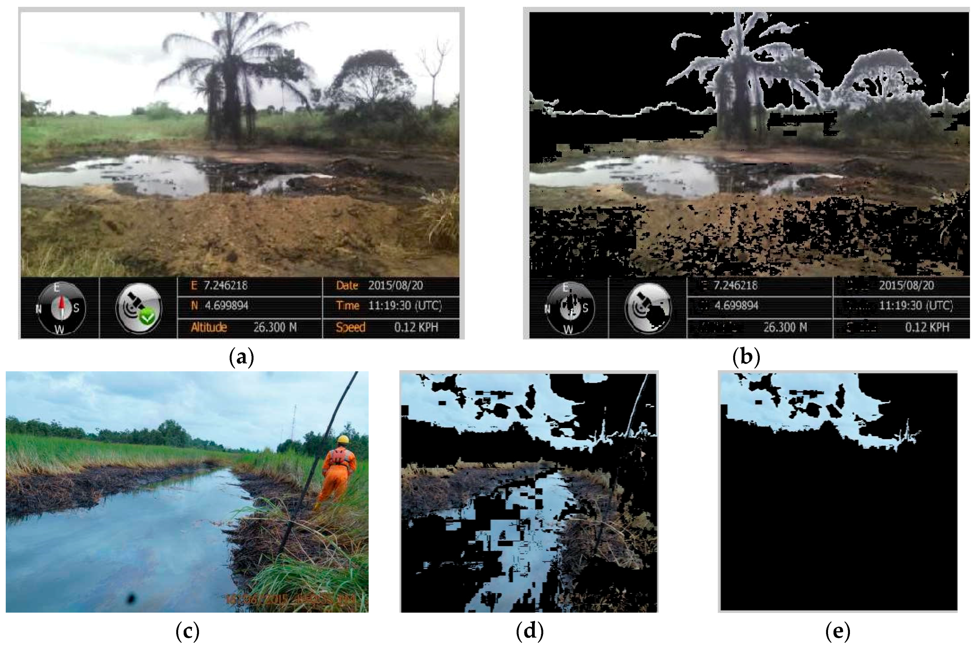
Sections of a crude oil spill image in which the sky is present are section in which there is no crude oil spill and therefore should not be considered as ROIs for further evaluation. In order to prevent the algorithm from flagging sky regions as ROIs, this section of the algorithm is dedicated to the detection and removal of these regions. By taking advantage of the fact that the sky is typically predominantly white or some shade of blue, the sky region, if present in an image, can be detected and removed. Figure 3d shows a crude oil spill in which the sky segmentation and removal section of the detection algorithm has been implemented. Because there are many different shades of blue, each with its own unique value in the RGB color spectrum, complete removal of the sky region in every image was not possible, as the spectrum of the blue color overlapped with other colors. In most cases, even a partial removal of the sky region was sufficient to prevent the algorithm from flagging it as a potential ROI.

For an Input Image, VSegmentedImage, the sky in the image is removed using the following procedure shown in Number 3 of the Appendix A. The values for S_T1A, S_T1B, S_T2A, S_T2B, S_T3A, and S_T3B were determined experimentally during the development of the algorithm using the sample cases. Afterwards, the optimal value for each of those parameters was utilized in the final algorithm and also for testing the algorithm on the sample cases. If a pixel, p(i,j), had its, R, G, and B, values within the minimum and maximum threshold identifying sky, then it is a pixel containing the sky and that pixel was eliminated by assigning it the RGB value for black (0,0,0). The output image SkySegmentedImage, was then passed on to the next stage of the algorithm.

2.2.4. ROI Extraction

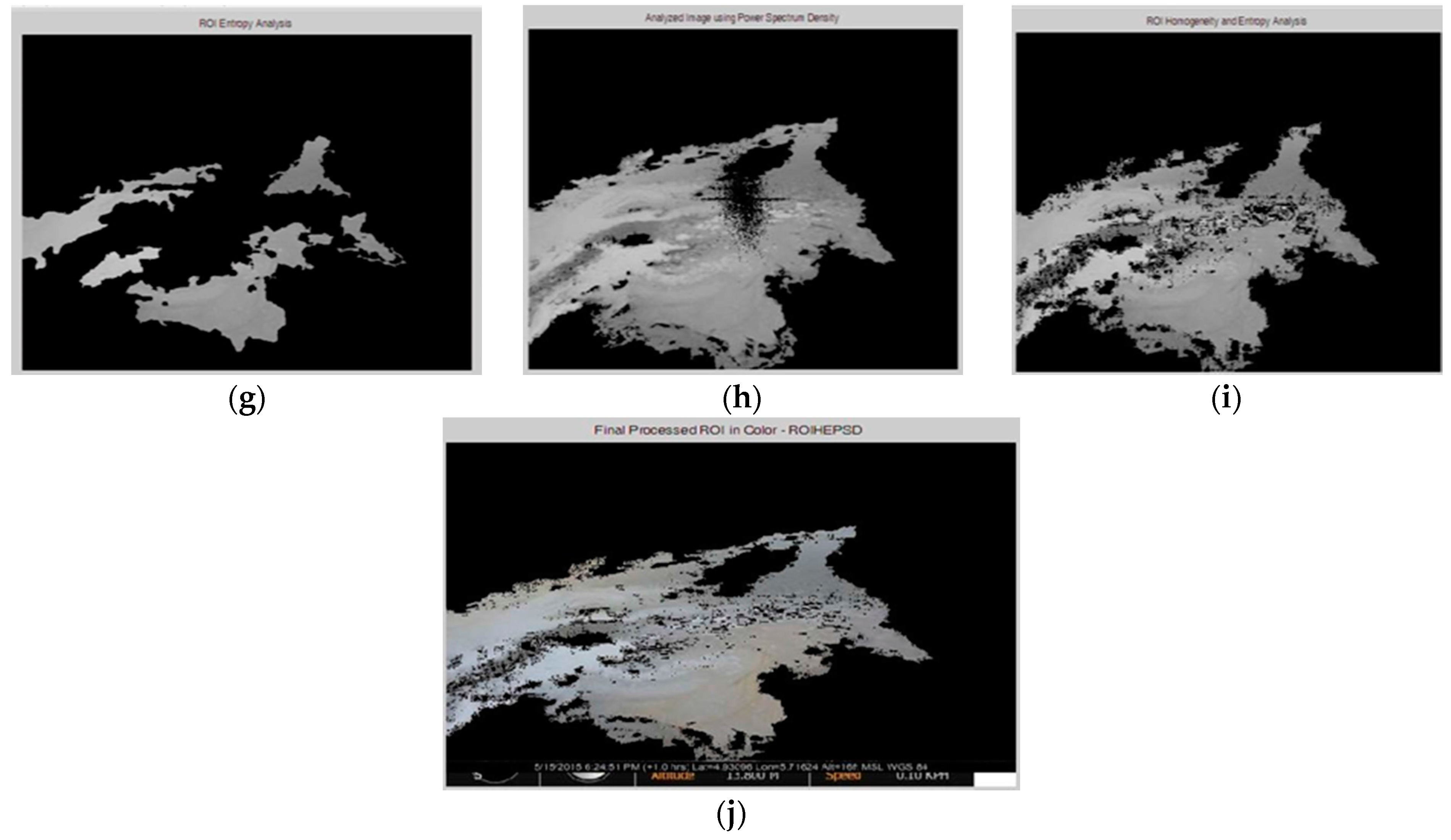
Identification of ROIs was performed on the grayscale image of the color segmented and sky-eliminated image. ROIs were determined by grouping interconnected pixels based on their grayscale values and proximity to one another. An experimentally determined threshold was utilized to determine if an ROI was to undergo further evaluation. If the area of an identified ROI was below a predetermined threshold, it was discarded. After successfully identifying ROIs with areas above this threshold, the ROI with the maximum area was then selected as the region on which further analysis was to be performed. Figure 3e shows the ROI selected in a case image for further processing. It is the ROI with the maximum area in the color-segmented and sky-eliminated image shown in Figure 3d.

For an Input Image, SkySegmentedImage, ROI was extracted using the following procedure shown in Number 4 of the Appendix A. The values for area threshold, A_T, was chosen experimentally during the development of the algorithm using the sample cases. Afterwards, the optimal value for each of those parameters was utilized in the final algorithm and also for testing the algorithm on the sample cases. The output image, ROI, was passed on to the next stage of the algorithm.

2.2.5. ROI Texture Feature Extraction

Certain texture features were computed and measured for each ROI identified by the algorithm. The selected features were homogeneity, entropy, and power spectrum density. Homogeneity is a measure of how close in the grayscale values of a pixel is when compared with its neighboring pixels. Using a window size of 3 × 3 pixels, the homogeneity for each pixel in the ROI image is computed. If the difference between the average grayscale value of the nine pixels in the window and the grayscale value of the center pixel is within a small range, then the central pixel is classified as a homogeneous pixel. If that difference is outside the range, then that pixel is determined to be non-homogeneous. Using this method, every pixel in the ROI image was classified as either homogeneous or non-homogeneous. The range for determining the homogeneity of a pixel was chosen experimentally. After homogeneity extraction, neighboring homogeneous pixels were grouped into ROIs and ROIs with areas above a certain threshold were selected for feature analysis. Figure 3f shows the homogeneity profile of the selected ROI region in Figure 3e. It was observed that majority of crude oil spills possessed homogeneous regions.

For an input image, ROI, the following procedure shown in Number 5 of the Appendix A was performed to extract homogeneous regions. The values for Homogeneity Threshold H_R, and Area Threshold, A_T, were determined experimentally during the development of the algorithm using the sample cases. Afterwards, the optimal value for each of those parameters was utilized in the final algorithm and also for testing the algorithm on the sample cases. The output image, FinalHImage, was passed on to the next stage of the algorithm.

Entropy is a measure of the amount of information that is needed for image compression. It measures the loss of information or message in a transmitted signal and also measured the image information [37]. The entropy was computed for the identified ROI using the entropyfilt function with a 3 × 3 pixel window size. After computation, pixels with an entropy value within a predetermined range were selected for further analysis. The acceptable entropy range used in selecting pixels for further analysis was determined experimentally with the sample images. Figure 3g shows the extracted entropy profile of the selected ROI region in Figure 3e.

For an input image, ROI, the following procedure shown in Number 5 of the Appendix A was performed to extract the entropy feature. The values for Entropy Threshold E_T1, and E_T2, were determined experimentally during the development of the algorithm using the sample cases, and they were defined as a percentage of the maximum entropy value in order to facilitate their application to other data sets of images. Afterwards, the optimal value for each of those parameters was utilized in the final algorithm and also for testing the algorithm on the sample cases. The output image, EImage2, was passed on to the next stage of the algorithm.

The power spectrum density (PSD) shows the strength of the variations (energy) as a function of frequency. It provides a representation of the amplitude of a surface’s roughness as a function of the spatial frequency of the roughness. After computation, pixels with a PSD value within a predetermined range were selected for further analysis. The acceptable range used in selecting pixels for further analysis was determined experimentally with the sample images. Figure 3h shows the extracted PSD profile of the selected ROI region in Figure 3e.

For an input image, ROI, the following procedure as shown in Number 5 of the Appendix A was performed to extract the PSD feature. The values for PSD Threshold PSD_T1, and PSD_T2, were determined experimentally during the development of the algorithm using the sample cases, and they were defined as a percentage of the maximum PSD value in order to facilitate their application to other data sets of images. Afterwards, the optimal value for each of those parameters was utilized in the final algorithm and also for testing the algorithm on the sample cases. The output image, PSDImage2, was passed on to the next stage of the algorithm.

2.2.6. ROI Texture Feature Analysis and Classification

The homogeneity, entropy and PSD ROIs for the ROI extracted from the original image were integrated into a final image containing regions flagged as crude oil spills. First, the homogeneity ROI (see Figure 3f) and entropy ROI (see Figure 3g) were combined by checking to see if a pixel was either homogeneous or if its entropy value fell within the specified acceptable range. If either of these conditions held true for a pixel, then it was selected for further processing, forming a new ROI with analyzed homogeneity and entropy features, as shown in Figure 3i.

The mean grayscale intensity value of the homogeneity and entropy ROI was used in thresholding the PSD ROI. The thresholded PSD ROI was then combined with the homogeneity and entropy ROI. If a pixel had a grayscale intensity value greater than zero in either the homogeneity and entropy ROI or the thresholded PSD ROI, it was classified as a pixel containing crude oil spill. Otherwise, it was classified as a non-crude oil spill pixel. In some images, the homogeneity and entropy ROI image contained multiple ROIs. When this happened, the algorithm thresholded the PSD ROI image using the mean grayscale intensity value for each ROI within the homogeneity and entropy image, then matched each ROI in the thresholded PSD ROI image with its corresponding ROI in the homogeneity and entropy image, before proceeding to integrate the data in the two images as described above. After integration, neighboring pixels are combined to form regions containing crude oil spills. Figure 3j shows the final detected crude oil spill from the original case image in Figure 3a.

For input images, FinalHImage, EImage2, and PSDImage2, the following procedure as shown in Number 6 of the Appendix A was performed to classify the ROI. The output image, OilSpill, is the final image containing the detected crude oil spill from the original image.

3. Results

The spill detection algorithm described above was developed using 25 sample images containing different volumes of crude oil spills. The results from testing the algorithm on these sample images are presented in Table 1. The algorithm successfully detected the crude oil spill in 23 of the 25 images, resulting in a sensitivity of 92%. The average False Positive per Image (FPI) was 1.43.

The final spill detection algorithm was tested on 56 case images. The results are presented in Table 2. The algorithm successfully detected the crude oil spill in 46 out of 56 images, resulting in a sensitivity of 82%. The average False Positive per Image (FPI) was 0.66.

4. Discussion

The spill detection algorithm developed in this paper demonstrated a sensitivity of 92% when tested on the set of sample images, and a sensitivity of 82% when tested on a set of sample cases. The algorithm also demonstrated high specificity for crude oil spills, with 1.43 and 0.66 FPI for the sample and sample cases respectively. This means that the algorithm is able to identify with a high degree of accuracy whether a spill is present in a given ROI. There were several challenges, however, that affected the algorithm’s ability to achieve 100% sensitivity.

The overlap of RGB range for various colors affected the efficiency of the algorithm during the color segmentation stage. In particular, the RGB range of values for the different shades of brown overlapped those for the color green. This made it difficult for the algorithm to effectively eliminate green vegetation during color segmentation. It was observed that the darker the shade of green, the more the algorithm was unable to eliminate the background vegetation during ROI identification and extraction. Figure 4a shows the sample image OS25, an image in which the algorithm failed to identify the crude oil spill. Figure 4b shows the color segmentation result for OS25. Most of the dark green trees and vegetation in the image are still present in the color-segmented image, making it difficult for the algorithm to select the initial ROI that would contain the crude oil spill.

Another factor that affected the efficiency of the spill detection algorithm was the color of the crude oil spill in the sample and case images. It was determined from the sample images that the color of the crude oil was predominantly brown. A predefined range of RGB values was used to segment out regions that could possibly contain crude oil. However, there were some images in which the color of the crude oil spill was not within the specified RGB range for brown used in the algorithm. Figure 5a shows a case image, OS46, in which the color of the crude oil spill is a mixture of orange and brown. The corresponding color segmented image is shown in Figure 5b, showing that only a small portion of the spill with dark brown color is segmented out as a possible ROI. This is the primary reason why the algorithm was unable to detect the crude oil spill in OS46. Similarly, the color of the crude oil spill in case image OS66 is outside the predefined RGB color range for crude oil, closer to black than brown (see Figure 5c), and is therefore not segmented out in the corresponding color segmentation image shown in Figure 5d. In fact, the crude oil spill is the only region segmented out in Figure 5d.

The sky detection and removal stage of the algorithm also encountered challenges in some spill images. Since the RGB range for various shades of blue overlapped with the range for other colors, only a restricted portion of the full RGB range for blue was selected for the detection of the sky region in a crude oil spill image (if present). This was in addition to the RGB range for the various shades of white.

Figure 6a shows a case image, OS63, and the result of the implementation of the algorithm’s sky detection and removal stage is shown in Figure 6b. For this particular case image, the algorithm successfully removed the entire sky region. However for the case image OS51, shown in Figure 6c, the algorithm only succeeded in removing a portion of the sky region (see Figure 6d). This led the algorithm to select the unsegmented sky region as the primary ROI for further analysis (see Figure 6e) and is the reason why the crude oil spill went undetected in this case image. Had a wider RGB range for blue been selected, it is possible that the sky detection and removal for OS51 would have been more successful and would have resulted in the accurate selection of the spill as the primary ROI as opposed to the unsegmented sky region selected in Figure 6e.

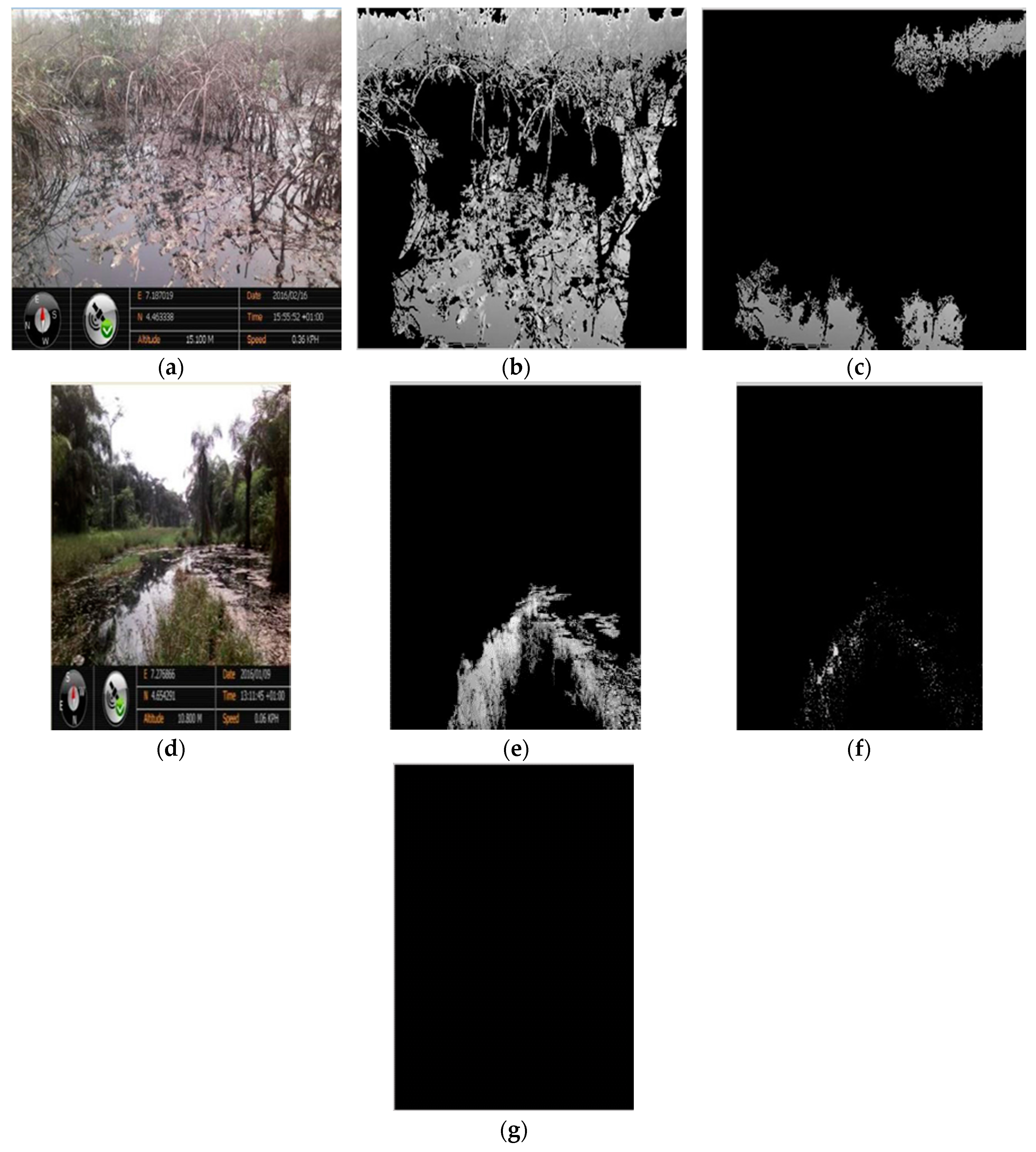
Even when the algorithm successfully identified the crude oil spill as its primary ROI for further analysis, the presence of weeds and other small vegetation among the spill affected the algorithm’s ability to classify that ROI as a crude oil spill. Figure 7a is sample image OS22 containing vegetation within the crude oil spill. Figure 7b shows the primary ROI selected after preprocessing and sky and color segmentation of OS22. The presence of vegetation affected the total area of the crude oil spill selected in the primary ROI. The total area of the final region identified as a crude oil spill in Figure 7c is far less than the area containing the spill in the original case image in Figure 7a. So although the algorithm was able to correctly identify the crude oil spill in the image, the area of the detected crude oil spill was severely impacted by the presence of vegetation. Figure 7d is sample image OS25, for which the algorithm failed to detect the crude oil spill. Note that the algorithm accurately selected the region containing the crude oil spill as its primary ROI for further analysis (see Figure 7e). However, the presence of the weeds among the spill lowered the homogeneity of the correctly identified primary ROI (see Figure 7f), so none of the homogeneous regions identified in the homogeneity analysis were above the set area threshold. As a result, no ROI was identified after the homogeneity analysis was completed (see Figure 7g), and therefore the spill in this image went undetected.

Another factor that affected the algorithm’s ability to detect crude oil spills in the images was the presence of reflections on the surface of the crude oil surface. When sunlight, vegetation and other objects cast their shadows on the surface of the spill, it alters the natural color of the spill, causing it to fall out of the defined RGB color range for crude oil spills and rendering the algorithm unable to identify such shadowed regions as crude oil spills. Figure 8a is the sample image OS8, which clearly shows a crude oil spill containing not only weeds, but also reflections of the surrounding vegetation, as well as reflections from the sunlight above. The detected crude oil spill from the OS8 is shown in Figure 9b. The algorithm was unable to detect the regions of the crude oil spill with vegetation reflections and weeds. This considerably reduced the area of the crude oil spill detected by the algorithm.

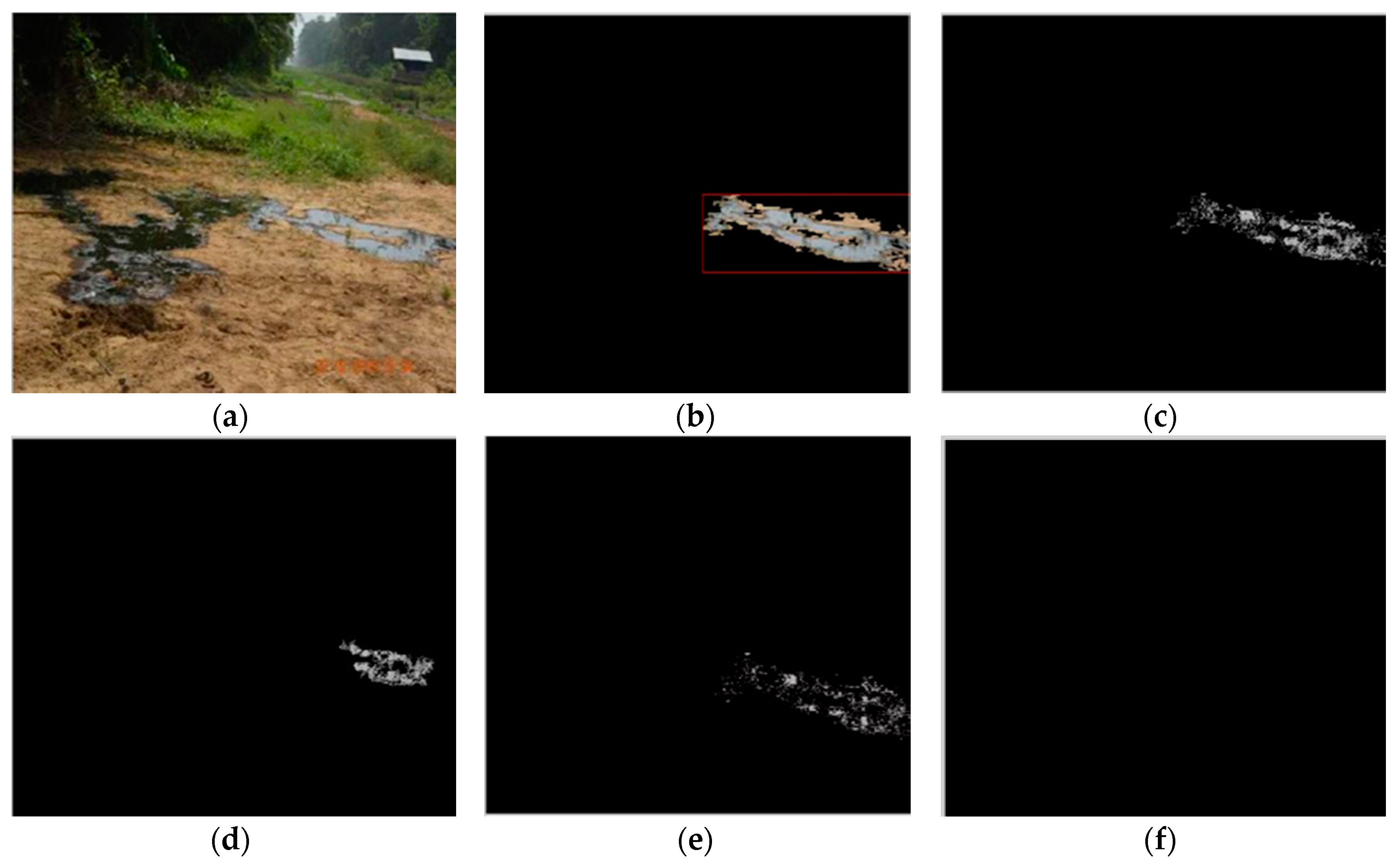
Another crucial factor that affected the algorithm’s ability to detect crude oil spills was the range of acceptable values chosen for determining the homogeneity of a pixel. Figure 9a is case image OS28. Figure 9b shows the primary ROI selected in OS28 for further analysis. Figure 9c shows the pixels whose grayscale intensity values fall within −5 and +5 of the average grayscale intensity values of their neighboring pixels in a 3 × 3 block. Figure 9d shows the homogeneity ROI extracted from Figure 9c. Figure 9e shows the pixels whose grayscale intensity values fall within −2 and +2 of the average grayscale intensity values of their neighboring pixels in a 3 × 3 block. Figure 9f shows the homogeneity ROI extracted from Figure 9e. The larger homogeneity range selected in Figure 9c enabled the algorithm to detect a portion of the crude oil spill and flag it as being homogeneous in Figure 9d. However, the smaller homogeneity range selected in Figure 9d for the analysis in Figure 9e identified very few pixels meeting that criteria, and as such, the algorithm could not identify any ROI that was homogeneous, as shown in Figure 9f. If the selected homogeneity range is too large, then the algorithm will flag non-crude oil spill regions as spill regions and this will increase the false positives flagged by the algorithm. The range selected for the homogeneity analysis is very important because if the algorithm does not identify a homogeneous ROI, then it will not flag any region in the image as a crude oil spill, regardless of the result of the entropy analysis and the PSD analysis.

There is a possibility that the presence of water puddles may affect the efficiency of the algorithm to a certain extent. However, the authors anticipate that the color of the water puddles will mostly lie outside the identified RGB range for crude oil and will therefore be eliminated during the Color Segmentation stage as well as the ROI extraction stage. Reflections on the surface of the water may also affect the algorithm’s performance in the same way the algorithm was affected by reflections on the surface of crude oil spills. Further tests will be conducted on images containing water to investigate the algorithm’s performance in eliminating water puddles and validating its specificity for crude oil spills. The spill detection algorithm developed in this article is intended to be employed by robotic oil spill surveillance systems that employ other methods to detect crude oil spills [48,49]. These systems primarily detect crude oil spills by means of gas sensors. However, after successful detection, they obtain and transmit spill images to relevant authorities using an on-board camera. The algorithm developed in this article can be integrated into this system as an additional step in spill verification and quantification.

Although the factors that affected the efficiency of the spill detection algorithm have been discussed in detail, the present algorithm also demonstrated good results for both the sample images and the case images. The specificity of the algorithm was extremely low, meaning that the algorithm displays a very high ability to discriminate between crude oil spills and non-crude oil spills once it has flagged the primary ROI for further analysis. It should be noted that the algorithm presently identifies only one primary ROI for analyzing the presence or absence of crude oil spill. If the algorithm is adjusted to analyze more than one primary ROI, then its sensitivity will improve considerably. This algorithm has demonstrated the ability to effectively detect the presence of crude oil spills in images, and can easily be incorporated into oil spill detection systems using visible sensors for quick and easy detection of crude oil spills.

5. Conclusions

Crude oil spills have negative consequences on the economy, environment, health and society in which they occur, and the severity of the consequences depends on how quickly these spills are detected once they begin. An algorithm for detecting and identifying crude oil spill in images captured with visible sensors has been developed and presented in this paper. The algorithm was developed using 25 sample images containing crude oil spills and demonstrated a sensitivity of 92% and an FPI of 1.43. The algorithm was further tested on a set of 56 case images and demonstrated a sensitivity of 82% and an FPI of 0.66. This algorithm can be incorporated into spill detection systems that utilize visible sensors for early detection of crude oil spills. Deep based learning oil spill detection can be explored as future work.

Author Contributions

O’tega Ejofodomi conceived the idea for this paper and was also responsible for developing and testing the algorithm used in this paper. Godswill Ofualagba was responsible for also developing and testing the algorithm used in this paper.

Conflicts of Interest

The authors declare no conflicts of interest.

Appendix A

1.
   Case (h = 681)
      PreprocessedImage = InitialImage(:,1:h − 100);
   Case (h = 844)
      PreprocessedImage = InitialImage (:,1:h − 70);
   end
 
2.
   For(int i = 1; i < w; i++)
      For(int j = 1; j < h; j++)
      If (PreprocessedImage(i,j,1) > V_T1A && PreprocessedImage(i,j,1) < V_T1B &&
          PreprocessedImage(i,j,2) >V_T2A && PreprocessedImage(i,j,2) < V_T2B &&
          PreprocessedImage(i,j,3) > V_T3A && PreprocessedImage(i,j,3) < V_T3B)
 
      VSegmentedImage(i,j,1) = 0;
      VSegmentedImage(i,j,2) = 0;
      VSegmentedImage(i,j,3) = 0;
  
      else
  
      VSegmentedImage(i,j,1) = PreprocessedImage(i,j,1);
      VSegmentedImage(i,j,2) = PreprocessedImage(i,j,2);
      VSegmentedImage(i,j,3) = PreprocessedImage(i,j,3);
 
      end
   end
 
where
w = Image width
h = Image height
V_T1A = minimum threshold for R component of green color identifying vegetation
V_T1B = maximum threshold for R component of green color identifying vegetation
V_T2A = minimum threshold for G component of green color identifying vegetation
V_T2B = maximum threshold for G component of green color identifying vegetation
V_T3A = minimum threshold for B component of green color identifying vegetation
V_T3B = maximum threshold for B component of green color identifying vegetation
 
3.
   For(int i = 1; i < w; i++)
       For(int j = 1; j < h; j++)
       If (VSegmentedImage(i,j,1) > S_T1A && VSegmentedImage (i,j,1) < S_T1B &&
           VSegmentedImage (i,j,2) >S_T2A && VSegmentedImage (i,j,2) < S_T2B &&
           VSegmentedImage (i,j,3) > S_T3A && VSegmentedImage (i,j,3) < S_T3B)
 
       SkySegmentedImage(i,j,1) = 0;
       SkySegmentedImage(i,j,2) = 0;
       SkySegmentedImage(i,j,3) = 0;
 
       else
 
       SkySegmentedImage(i,j,1) = VSegmentedImage(i,j,1);
       SkySegmentedImage(i,j,2) = VSegmentedImage(i,j,2);
       SKySegmentedImage(i,j,3) = VSegmentedImage(i,j,3);
 
      end
   end
 
where
w = Image width
h = Image height
S_T1A = minimum threshold for R component of blue and white color identifying sky
S_T1B = maximum threshold for R component of blue and white color identifying sky
S_T2A = minimum threshold for G component of blue and white color identifying sky
S_T2B = maximum threshold for G component of blue and white color identifying sky
S_T3A = minimum threshold for B component of blue and white color identifying sky
S_T3B = maximum threshold for B component of blue and white color identifying sky
 
4.
   maxI = 0;
   GSkySegmentedImage = rgb2gray(SkySegmentedImage);
   ROIImage = bwlabel(SkySegmentedImage);
   Stats = regionprops(ROIImage, ‘Area’);
   idx = find([stats.Area] > A_T;
   BW2 = ismember(labelmatrix(ROIImage), idx);
   for(int i= 1; i <= idx; i++)
   if maxI < idx(i).Area
     maxI = idx(i);
   end
   ROI = ismember(labelmatrix(ROIImage), maxI);
    
A_T = minimum threshold for size of ROI Area
 
5.
   For(int i = 2; i< w − 1; i++)
      For(int j = 2; j < h − 1; j+++)
	   
      average =round {[ p(i,j) + p(i − 1,j) + p(I + 1,j) + p(i,j − 1) + p(i,j + 1) + p(i − 1,j − 1) + p(i − 1,j + 1) + p(i+1,j − 1)
                   + p(I + 1,j + 1)]/9};
      If(abs(average – p(I,j)) < H_R
         HImage(i,j) = ROI(i,j);
      else
         HImage = 0;
      end
     end
   end
 
   HImage2 = bwlabel(HImage);
   Stats = regionprops(HImage2, ‘Area’);
   idx = find([stats.Area] > A_T;
   BW2 = ismember(labelmatrix(HImage2), idx);
   for(int i= 1; i <= idx; i++)
   if maxI < idx(i).Area
      maxI = idx(i);
   end
   FinalHImage = ismember(labelmatrix(HImage2), maxI);
   
H_R = Homogeneity Threshold
 
EImage = entropyfilt(ROI);
For(int i = 1; i< w; i++)
   For(int j = 1; j < h; j+++)
	 
   If(EImage(i,j) > E_T1  and EImage(i,j) < E_T2)
         EImage2(i,j) = ROI(i,j);
   else
         EImage2(i,j) = 0;
   end
   end
end
 
E_T1 = minimum threshold for Entropy, expressed as a percentage of maximum Entropy Value in Image
E_T2 = maximum threshold for Entropy, expressed as a percentage of maximum Entropy Value in Image
 
PSDImage = log10(abs(fftshif(fft2(ROI))).^2));
For(int i = 1; i< w; i++)
   For(int j = 1; j < h; j+++)
   
    If(PSDImage(i,j) > PSD_T1  and PSDImage(i,j) < PSD_T2)
         PSDImage2(i,j) = ROI(i,j);
    else
         PSDImage2(i,j) = 0;
    end
    end
end
 
PSD_T1 = minimum threshold for PSD, expressed as a percentage of maximum PSD Value in Image
PSD_T2 = maximum threshold for PSD, expressed as a percentage of maximum PSD Value in Image
    
6.
For(int i = 1; i< w; i++)
    For(int j = 1; j < h; j+++)
        If (FinalHImage(i,j) > 0) || (EImage2(i,j) > 0)
             ROHE(i,j) = ROI(i,j);
        else
             ROHE(i,j) = 0;
        end
    end
end
ROHEmean = mean(mean(ROHE));
For(int i = 1; i< w; i++)
    For(int j = 1; j < h; j+++)
        If (PSDImage2(i,j) > ROHEmean)
             TPSDImage(i,j) = PSDImage2(i,j);
        else
             TPSDImage(i,j) = 0;
        end
    end
end
 
For(int i = 1; i< w; i++)
    For(int j = 1; j < h; j+++)
        If (ROHE(i,j) > 0) || (TPSDImage(i,j) > 0)
             OilSpill(i,j) = ROI(i,j);
        else
             OilSpill(i,j) = 0;
        end
    end
end

References

Chang, S.E.; Stone, J.; Demes, K.; Piscitelli, M. Consequences of oil spills: A review and framework for informing planning. Ecol. Soc. 2014, 19, 26. [Google Scholar] [CrossRef]
D’Andrea, M.A.; Kesava, G.R. Health Consequences among Subjects Involved in Gulf Oil Spill Clean-up Activities. Am. J. Med. 2013, 126, 966–974. [Google Scholar] [CrossRef] [PubMed]
Oyebamiji, M.A.; Mba, I.C. Effects of Oil Spillage on Community Development in the Niger Delta Region: Implications for the Eradication of Poverty and Hunger (Millennium Development Goal One) in Nigeria. World J. Soc. Sci. 2014, 1, 27–36. [Google Scholar]
Okoye, C.O.; Okunrobo, L.A. Impact of Oil Spill on Land and Water and its Health Implications in Odugboro Community, Sagamu, Ogun State, Nigeria. World J. Environ. Sci. Eng. 2014, 1, 1–21. [Google Scholar]
Zaki, M.S.; Authman, M.M.N.; Ata, N.S. Effects of Environmental Oil Spills on Commercial Fish and Shellfish in Suez Canal and Suez Gulf Regions. Life Sci. J. 2014, 11, 269–274. [Google Scholar]
Oyem, I.L. Effects of Crude Oil Spillage on Soil Physico-Chemical Properties in Ugborodo Community. Int. J. Mod. Eng. Res. 2013, 3, 3336–3342. [Google Scholar]
Mogborukor, J.O.A. The Impact of Oil Exploration and Exploitation on Water Quality and Vegetal Resources in a Rain Forest Ecosystem of Nigeria. Mediterr. J. Soc. Sci. 2014, 5, 1678–1685. [Google Scholar] [CrossRef]
Kadafa, A.A. Oil Exploration and Spillage in the Niger Delta of Nigeria. Civ. Environ. Res. 2012, 2, 38–51. [Google Scholar]
Melanie, D. Exxon Valdez Oil Spill Continued Effects on the Alaskan Economy. Colon. Acad. Alliance Undergrad. Res. J. 2010, 1, 7. [Google Scholar]
Nwachukwu, A.N.; Osuagwu, J.C. Effects of Oil Spillage on Groundwater Quality in Nigeria. Am. J. Eng. Res. 2014, 3, 271–274. [Google Scholar]
Etkin, D.S. Analysis of U.S. Oil Spillage. Available online: http://www.api.org/environmenthealth-and-safety/clean-water/oil-spill-prevention-and-response/~/media/93371edfb94c4b4d9c6bbc766f0c4a40.ashx (accessed on 13 June 2016).
Statistical Summary Pipeline Occurrences 2014. Available online: http://www.tsb.gc.ca/eng/stats/pipeline/2014/ssep-sspo-2014.asp (accessed on 13 July 2016).
Nigerian Oil Industry Annual Statistics Bulletin 2012. Department of Petroleum Resources. Available online: https://dpr.gov.ng/index/wp-content/uploads/2014/10/2012-INDUSTRY-STATISTICAL-BULLETIN.pdf (accessed on 13 July 2016).
Ormseth, O.A.; Ben-David, M. Ingestion of crude oil: Effects on digesta retention times and nutrient uptake in captive river otters. J. Comp. Physiol. 2000, 170, 419–428. [Google Scholar] [CrossRef]
Rogers, V.V.; Wickstrom, M.; Liber, K.; MacKinnon, M.D. Acute and subchronic mammalian toxicity of naphthenic acids from oil sands tailings. Toxicol. Sci. 2002, 66, 347–355. [Google Scholar] [CrossRef] [PubMed]
Ma, J.Y.C.; Rengasamy, A.; Frazer, D.; Barger, M.W.; Hubbs, A.F.; Battelli, L.; Tomblyn, S.; Stone, S.; Castranova, V. Inhalation exposure of rats to asphalt fumes generated at paving temperatures alters pulmonary xenobiotic metabolism pathways without lung injury. Environ. Health Perspect. 2003, 111, 1215–1221. Available online: http://www.ncbi.nlm.nih.gov/pmc/articles/PMC1241577/ (accessed on 13 July 2016). [CrossRef] [PubMed]
Kazlauskiene, N.; Vosyliene, M.Z.; Ratkelyte, E. The comparative study of the overall effect of crude oil on fish in early stages of development. In Dangerous Pollutants (Xenobiotics) in Urban Water Cycle, Proceedings of the NATO Advanced Research Workshop on Dangerous Pollutants (Xenobiotics) in Urban Water Cycle, Lednice, Czech Republic, 3–6 May 2007; Hlavinek, P., Bonacci, O., Marsalek, J., Mahrikova, I., Eds.; Springer: Amsterdam, The Netherlands, 2007; pp. 307–316. [Google Scholar]
Incardona, J.P.; Carls, M.G.; Day, H.L.; Sloan, C.A.; Bolton, J.L.; Collier, T.K.; Scholz, N.L. Cardiac arrhythmia is the primary response of embryonic Pacific herring (Clupea pallasi) exposed to crude oil during weathering. Environ. Sci. Technol. 2009, 43, 201–207. [Google Scholar] [CrossRef] [PubMed]
Aguilera, F.; Mendez, J.; Pasaro, E.; Laffon, B. Review on the effects of exposure to spilled oils on human health. J. Appl. Toxicol. 2010, 30, 291–301. [Google Scholar] [CrossRef] [PubMed]
Judson, R.S.; Martin, M.T.; Reif, D.M.; Houck, K.A.; Knudsen, T.B.; Rotroff, D.M.; Xia, M.; Sakamuru, S.; Huang, R.; Shinn, P.; et al. Analysis of Eight Oil Spill Dispersants Using Rapid, In Vitro Tests for Endocrine and Other Biological Activity. Environ. Sci. Technol. 2010, 44, 5979–5985. [Google Scholar] [CrossRef] [PubMed]
Major, D.N.; Wang, H. How public health impact is addressed: A retrospective view on three different oil spills. Toxicol. Environ. Chem. 2012, 94, 442–467. [Google Scholar] [CrossRef]
Chindah, C.A.; Braide, A.S. The Impact of Oil Spills on the Ecology and Economy of the Niger Delta. In Proceedings of the Workshop on Sustainable Remediation Development Technology; Institute of Pollution Studies, River State University of Science and Technology: Port-Harcourt, Nigeria, 2000. [Google Scholar]
Inoni, O.; Douglason, E.; Omotor, G.; Adun, F.N. The Effect of Oil Spillage on Crop Yield and Farm Income in Delta State, Nigeria. J. Cent. Eur. Agric. 2006, 7, 41–48. Available online: https://jcea.agr.hr/articles/315_THE_EFFECT_OF_OIL_SPILLAGE_ON_CROP_YIELD_AND_FARM_INCOME_IN_DELTA_STATE_NIGERIA_en.pdf (accessed on 13 July 2016).
Zabbey, N. Impacts of Oil Pollution on Livelihoods in Nigeria. In Proceedings of the Confenrence on Petroleum and Pollution—How Does That Impact Human Rights? Amnesty International, Friends of the Earth: Stockholm, Sweden, 2010; Available online: http://www.cehrd.org/files/Oil_and_livelihoods_in_the_Niger_Delta.pdf (accessed on 13 July 2016).
Gay, J.; Shepherd, O.; Whitman, M.; Thyden, M. The Health Effects of Oil Contamination: A Compilation of Research. Worcester Polytechnic Institute, 2010. Available online: https://web.wpi.edu/Pubs/E-project/Available/E-project-121510-203112/unrestricted/Health_Effects_of_Oil_Contamination_-_Final_Report.pdf (accessed on 13 July 2015).
Salako, A.; Oluwafolahan, S.; Sunkanmi, A. Oil Spills and Community Health: Implications for Resource Limited Settings. J. Toxicol. Environ. Health Sci. 2012, 4, 145–150. [Google Scholar] [CrossRef]
Rodriguez-Trigo, G.; Zock, J.P.; Montes, I.I. Health effects of exposure to oil spills. Arch. Bronconeumol. 2007, 43, 628–635. [Google Scholar] [CrossRef]
Zock, J.P.; Rodriguez-Trigo, G.; Pozo-Rodriguez, F.; Barbera, J.A.; Bouso, L.; Torralba, Y.; Anto, J.M.; Gomez, F.P.; Fuster, C.; Verea, H. Prolonged respiratory symptoms in clean-up workers of the Prestige oil spill. Am. J. Respir. Crit. Care Med. 2007, 176, 610–616. [Google Scholar] [CrossRef] [PubMed]
Nigerian National Petroleum Company. Annual Statistical Bulletin. 2014. Available online: http://www.nnpcgroup.com/PublicRelations/OilandGasStatistics/AnnualStatisticsBulletin.aspx (accessed on 13 July 2016).
Krisberg, K. Effect on Workers. Available online: http://thenationshealth.aphapublications.org/content/40/6/1.1.full (accessed on 10 September 2015).
Shirvany, R.; Chabert, M.; Tourneret, J. Ship and Oil-Spill Detection Using the Degree of Polarization in Linear and Hybrid/Compact Dual-Pol SAR. IEEE J. Sel. Top. Appl. Earth Obs. Remote Sens. 2012, 5, 885–892. [Google Scholar] [CrossRef] [Green Version]
Brekke, C.; Solberg, A.H.S. Oil Spill Detection by Satellite Remote Sensing. Remote Sens. Environ. 2005, 95, 1–13. [Google Scholar] [CrossRef]
Li, H.; Shen, C. Object-Respecting Color Image Segmentation. In Proceedings of the IEEE International Conference on Image Processing, San Antonio, TX, USA, 16 September–19 September 2007. [Google Scholar] [CrossRef]
Allili, M.S.; Ziou, D. An automatic Segmentation of Color Images by Using a Combination of Mixture Modelling and adaptive Region Information: A level set approach. In Proceedings of the IEEE International Conference on Image Processing, Genova, Italy, 11–14 September 2005. [Google Scholar] [CrossRef]
Cossu, R.; Chiappini, L. A Color Image Segmentation Method as used in the study of ancient monument decay. J. Cult. Heritage 2005, 5, 385–391. [Google Scholar] [CrossRef]
Otsu, N. A threshold selection method from gray-level histograms. IEEE Trans. SMC 1978, 8, 62–66. [Google Scholar] [CrossRef]
Canny, J. A computational approach to edge detection. IEEE Trans. PAMI 1986, 8, 679–698. [Google Scholar] [CrossRef]
Boroujeni, N.S.; Eternad, S.A.; Whitehead, A. Robust Horizon Detection Using Segmentation for UAV Applications. In Proceedings of the 9th Conference on Computer and Robot Vision (CRV), Toronto, ON, Canada, 28–30 May 2012. [Google Scholar] [CrossRef]
Topouzelis, K.N. Oil Spill Detection by SAR Images: Dark Formation Detection, Feature Extraction and Classification Algorithms. Sensors 2008, 8, 6642–6659. [Google Scholar] [CrossRef] [PubMed] [Green Version]
Solberg, A.; Storvik, G.; Solberg, R.; Volden, E. Automatic Detection of Oil Spills in ERS SAR Images. IEEE Trans. Geosci. Remote Sens. 1999, 37, 1916–1924. [Google Scholar] [CrossRef]
Del Frate, F.; Petrocchi, A.; Lichtenegger, J.; Calabresi, G. Neural networks for oil spill detection using ERS-SAR data. IEEE Trans. Geosci. Remote Sens. 2000, 5, 2282–2287. [Google Scholar] [CrossRef]
Espedal, H.A.; Wahl, T. Satellite SAR oil spill detection using wind history information. Int. J. Remote Sens. 1999, 20, 49–65. [Google Scholar] [CrossRef]
Espedal, H.A.; Johannessen, J.A. Detection of oil spills near offshore installations using synthetic aperture radar (SAR). Int. J. Remote Sens. 2000, 11, 2141–2144. [Google Scholar] [CrossRef]
Fiscella, B.; Giancaspro, A.; Nirchio, F.; Trivero, P. Oil Spill Detection using Marine SAR Images. Int. J. Remote Sens. 2000, 21, 3561–3566. [Google Scholar] [CrossRef]
De Souza, D.; Neto, A.; Da Mata, W. Intelligent System for Feature Extraction of Oil Slicks in SAR Images: Speckle Filter Analysis. In Proceedings of the 13th International Conference on Neural Information Processing (ICONIP 2006), Hong Kong, China, 3–6 October 2006. [Google Scholar]
Serra-Sogas, N.; O’Hara, P.D.; Canessa, R.; Keller, P.; Pelot, R. Visualization of Spatial Patterns and Temporal Trends for Aerial Surveillance of Illegal Oil Discharges in Western Canadian Marine Waters. Mar. Pollut. Bull. 2008, 56, 825–833. [Google Scholar] [CrossRef] [PubMed]
Shell Nigeria. Available online: www.shell.com.ng (accessed on 13 July 2016).
Ejofodomi, O.; Ofualagba, G. Exploring the Feasibility of Robotic Pipelilne Surveillance for Detecting Crude Oil Spills in the Niger Delta. Int. J. Unmanned Syst. Eng. 2017, 5, 8–52. [Google Scholar] [CrossRef]
Ejofodomi, O.; Ofualagba, G. Development of an Aerial Robotic Oil Spill Surveillance (AROSS) System for Constant Surveillance and Detection of Spills from Crude Oil Pipelines. Int. J. Unmanned Syst. Eng. 2016, 4, 19–33. [Google Scholar] [CrossRef]

Figure 1. Land Crude Oil Spill Images. (a) Sample image from sample images; (b) Sample Images from Case Images.

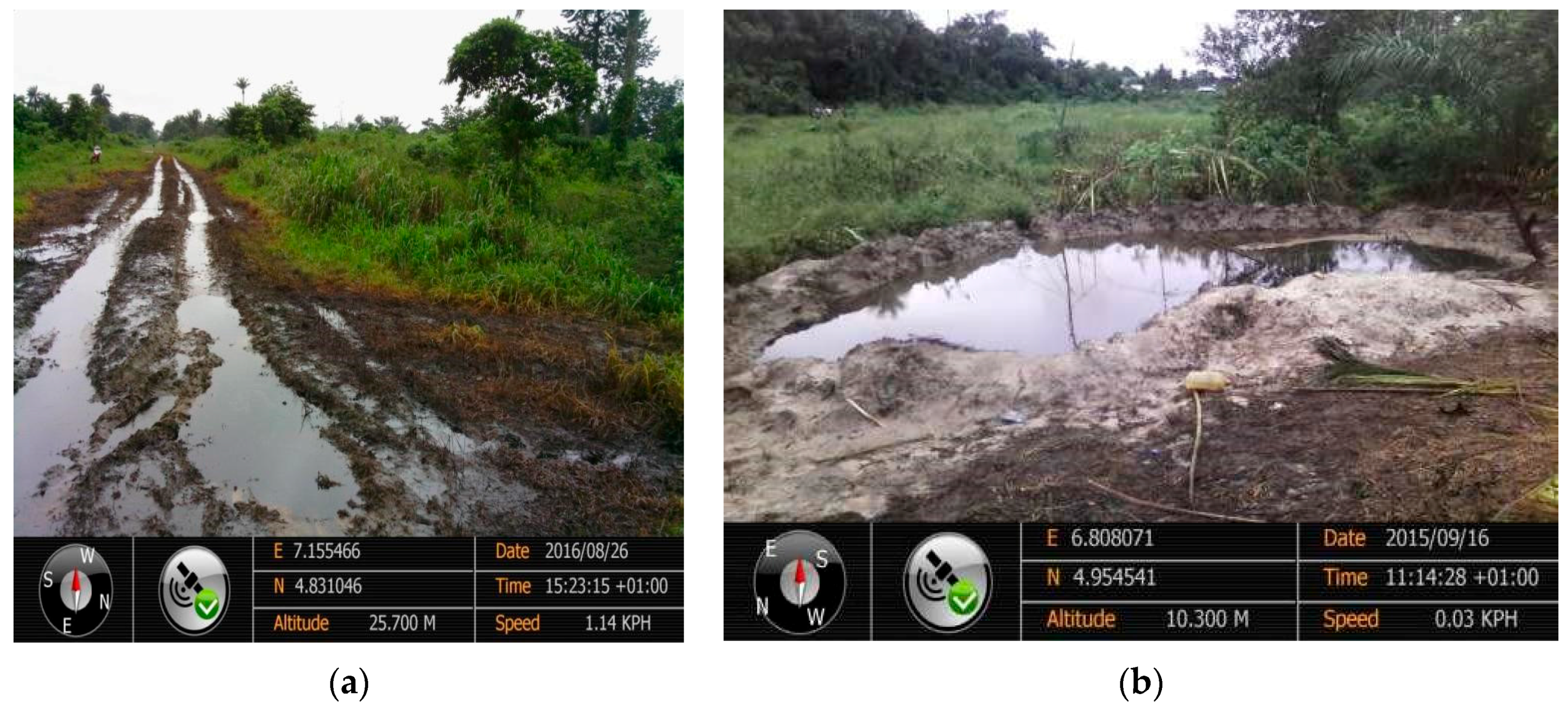
Figure 2. Land Crude Oil Spill Detection Algorithm.

Figure 3. Oil Spill Detection Algorithm Implementation on Case Image OS69. (a) Case Image OS69; (b) Preprocessed image; (c) Color Segmentation Image; (d) Sky Segmentation Image; (e) Selected Primary ROI; (f) ROI homogeneity Image; (g) Entropy Image; (h) PSD image; (i) ROI homogeneity and entropy features; (j) Detected Crude Oil Spill from OS69.

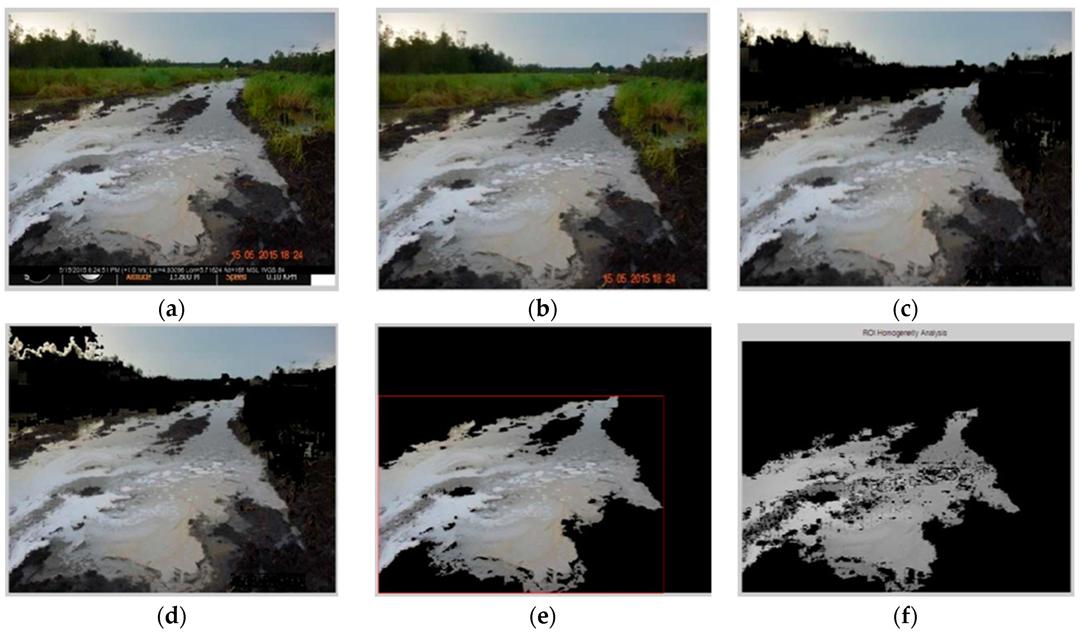
Figure 4. Effect of RGB color range overlap on color segmentation stage in spill detection algorithm. (a) Sample image OS25 with negative spill detection result; (b) Color Segmentation result for OS25 showing algorithm’s failure to eliminate dark green vegetation.

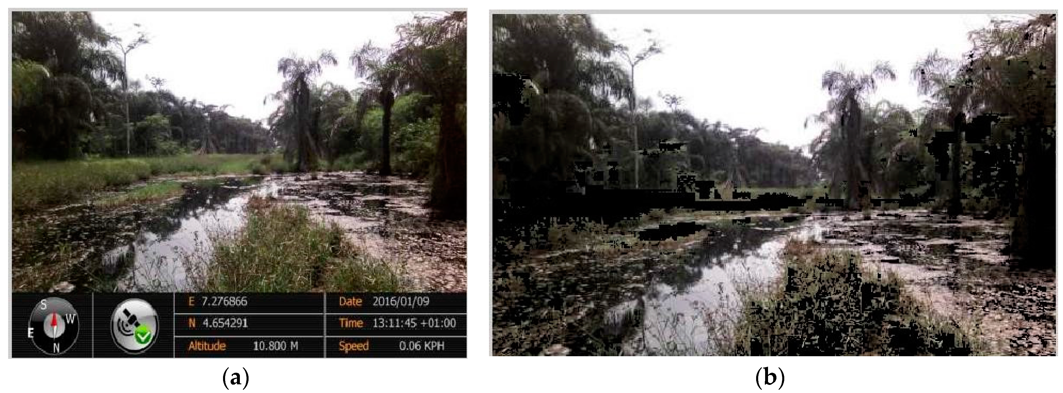
Figure 5. (a) Case image OS46; (b) Color Segmentation image for OS46; (c) Case Image OS66; (d) Color Segmentation image for OS66.

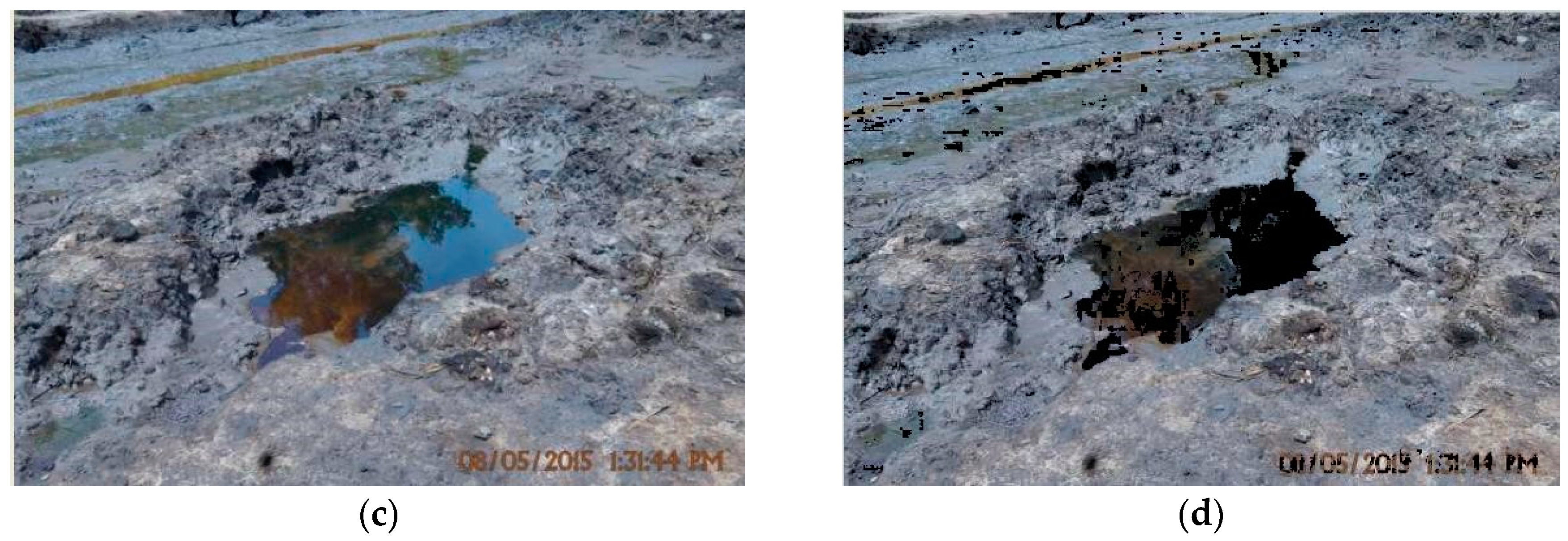
Figure 6. Sky Detection and Removal Stage. (a) Case Image OS63; (b) Effective Sky Detection and Removal for OS63; (c) Case Image OS51; (d) Ineffective Sky Detection and Removal for OS51; (e) Selection of Sky Region as primary ROI for OS51.

Figure 7. Effect of Weeds on Crude Oil Spill Detection. (a) Sample Image OS22; (b) primary ROI for OS22 after preprocessing, and sky and color segmentation removal; (c) Identified Crude Oil Spill from OS22; (d) Sample Image OS25; (e) Primary ROI for OS25 after preprocessing, and sky and color segmentation removal; (f) Homogeneity Analysis Result for OS25; (g) Identified Homogeneity ROI for OS25.

Figure 8. (a) Sample Image OS9; (b) Detected crude oil spill from OS9.

Figure 9. (a) Case Image OS28; (b) Primary ROI in OS28 identified for further analysis; (c) Pixels meeting homogeneity range of Mean −5 to Mean +5; (d) Final Homogeneity ROI derived from (c); (e) Pixels meeting homogeneity range of Mean −2 to Mean +2; (f) Final Homogeneity ROI derived from (e).

Table 1. Spill Detection Algorithm Results on Sample Images.

Sample Image No.	Successful Spill Detection	No. of False Positives (FP)
OS1	YES	0
OS2	YES	0
OS5	YES	4
OS7	YES	0
OS8	YES	0
OS9	NO	0
OS10	YES	2
OS11	YES	2
OS14	YES	1
OS18	YES	3
OS19	YES	0
OS20	YES	0
OS21	YES	0
OS22	YES	2
OS23	YES	0
OS25	NO	0
OS2b	YES	1
OS5b	YES	7
OS9b	YES	3
OS12b	YES	5
OS16b	YES	1
OS19b	YES	0
OS20b	YES	2
OS22b	YES	0
OS24b	YES	0

Table 2. Spill Detection Algorithm Results on Case Images.

Sample Image No.	Successful Spill Detection	No. of False Positives (FP)
OS26	YES	2
OS27	YES	1
OS28	YES	0
OS28b	NO	0
OS29	YES	0
OS31	NO	1
OS32	YES	1
OS32b	YES	0
OS33	YES	0
OS34	NO	2
OS34b	YES	1
OS35	YES	0
OS36	YES	3
OS36b	YES	1
OS37	YES	1
OS38	YES	2
OS38b	YES	2
OS38c	YES	3
OS39	YES	0
OS40	YES	0
OS41	NO	0
OS42	YES	1
OS42b	YES	0
OS43	YES	3
OS44	YES	0
OS46	NO	0
OS48	NO	0
OS48b	YES	1
OS49	YES	0
OS49b	YES	0
OS50	YES	0
OS51	YES	0
OS52	YES	0
OS53	NO	3
OS54	YES	0
OS55	YES	0
OS56	YES	0
OS57	YES	0
OS58	YES	0
OS59	YES	0
OS60	YES	1
OS61	NO	2
OS61b	YES	1
OS62	NO	0
OS63	YES	1
OS63b	YES	0
OS64	YES	1
OS65b	YES	1
OS67	YES	1
OS68	YES	0
OS69	YES	0
OS69b	YES	1
OS70	NO	0
OS71	YES	0
OS74	YES	2
OS75	YES	0

© 2017 by the authors. Licensee MDPI, Basel, Switzerland. This article is an open access article distributed under the terms and conditions of the Creative Commons Attribution (CC BY) license (http://creativecommons.org/licenses/by/4.0/).

Share and Cite

MDPI and ACS Style

Ejofodomi, O.; Ofualagba, G. Detection and Classification of Land Crude Oil Spills Using Color Segmentation and Texture Analysis. J. Imaging 2017, 3, 47. https://doi.org/10.3390/jimaging3040047

AMA Style

Ejofodomi O, Ofualagba G. Detection and Classification of Land Crude Oil Spills Using Color Segmentation and Texture Analysis. Journal of Imaging. 2017; 3(4):47. https://doi.org/10.3390/jimaging3040047

Chicago/Turabian Style

Ejofodomi, O’tega, and Godswill Ofualagba. 2017. "Detection and Classification of Land Crude Oil Spills Using Color Segmentation and Texture Analysis" Journal of Imaging 3, no. 4: 47. https://doi.org/10.3390/jimaging3040047

Note that from the first issue of 2016, this journal uses article numbers instead of page numbers. See further details here.

Article Menu

Detection and Classification of Land Crude Oil Spills Using Color Segmentation and Texture Analysis

Abstract

1. Introduction

2. Materials and Methods

2.1. Materials

2.2. Methods

2.2.1. Image Preprocessing

2.2.2. Color Segmentation

2.2.3. Sky Segmentation and Elimination

2.2.4. ROI Extraction

2.2.5. ROI Texture Feature Extraction

2.2.6. ROI Texture Feature Analysis and Classification

3. Results

4. Discussion

5. Conclusions

Author Contributions

Conflicts of Interest

Appendix A

References

Share and Cite

Article Metrics

Article Access Statistics

Further Information

Guidelines

MDPI Initiatives

Follow MDPI