Article

Transcription of Spanish Historical Handwritten Documents with Deep Neural Networks

by
Emilio Granell
1,*,
Edgard Chammas
2,
Laurence Likforman-Sulem
3,
Carlos-D. Martínez-Hinarejos
1,
Chafic Mokbel
2 and
Bogdan-Ionuţ Cîrstea
3
1
PRHLT Research Center, Universitat Politècnica de València, 46022 València, Spain
2
Department of Computer Engineering, University of Balamand, 2960 Balamand, Lebanon
3
Institut Mines-Télécom/Télécom ParisTech, Université Paris-Saclay, 75013 Paris, France
*
Author to whom correspondence should be addressed.
J. Imaging 2018, 4(1), 15; https://doi.org/10.3390/jimaging4010015
Submission received: 30 October 2017 / Revised: 22 December 2017 / Accepted: 2 January 2018 / Published: 11 January 2018
(This article belongs to the Special Issue Document Image Processing)

Abstract

:
The digitization of historical handwritten document images is important for the preservation of cultural heritage. Moreover, the transcription of text images obtained from digitization is necessary to provide efficient information access to the content of these documents. Handwritten Text Recognition (HTR) has become an important research topic in the areas of image and computational language processing that allows us to obtain transcriptions from text images. State-of-the-art HTR systems are, however, far from perfect. One difficulty is that they have to cope with image noise and handwriting variability. Another difficulty is the presence of a large amount of Out-Of-Vocabulary (OOV) words in ancient historical texts. A solution to this problem is to use external lexical resources, but such resources might be scarce or unavailable given the nature and the age of such documents. This work proposes a solution to avoid this limitation. It consists of associating a powerful optical recognition system that will cope with image noise and variability, with a language model based on sub-lexical units that will model OOV words. Such a language modeling approach reduces the size of the lexicon while increasing the lexicon coverage. Experiments are first conducted on the publicly available Rodrigo dataset, which contains the digitization of an ancient Spanish manuscript, with a recognizer based on Hidden Markov Models (HMMs). They show that sub-lexical units outperform word units in terms of Word Error Rate (WER), Character Error Rate (CER) and OOV word accuracy rate. This approach is then applied to deep net classifiers, namely Bi-directional Long-Short Term Memory (BLSTMs) and Convolutional Recurrent Neural Nets (CRNNs). Results show that CRNNs outperform HMMs and BLSTMs, reaching the lowest WER and CER for this image dataset and significantly improving OOV recognition.

1. Introduction

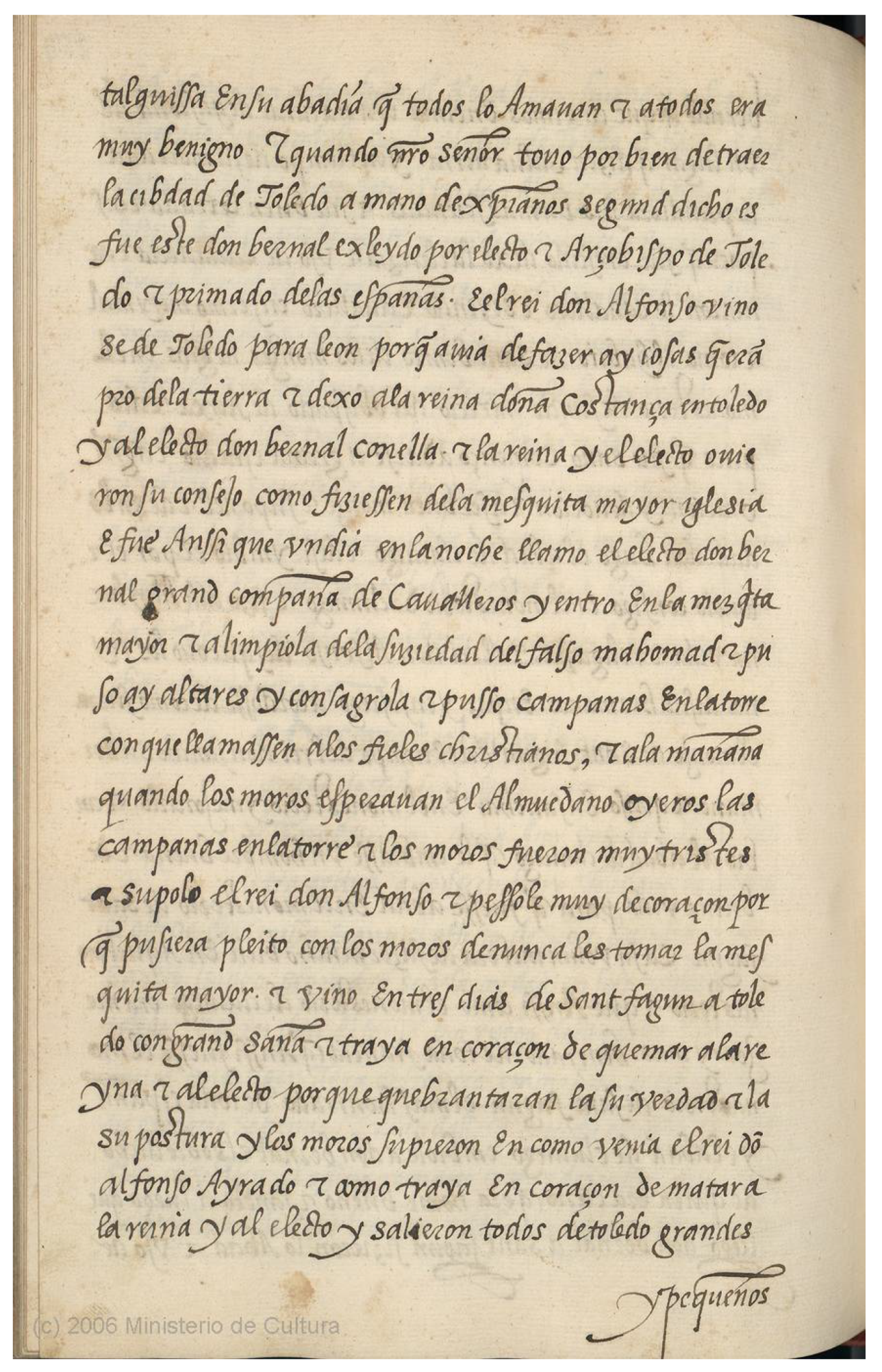
The digitization of historical handwritten document images is important for the preservation of cultural heritage. Moreover, the transcription of text images obtained from digitization is necessary to provide efficient information access to the content of these documents. Automatic transcription of these documents is performed by Handwriting Text Recognition (HTR) systems, which are traditionally composed of an optical model, a dictionary and a Language Model (LM). However, HTR systems face several challenges at both the image and language modeling levels. Historical document images may include defects due to age, manipulation and bleed-through of ink. They may also include calligraphic initial letters and long character strokes as ornaments. This is particularly true for Spanish documents from the 16th century as seen in Figure 1. Ancient texts also include rare characters, grammatical forms, word spellings and named entities distinct from modern ones. Such forms lead to Out-Of-Vocabulary (OOV) words, i.e., words that do not belong to the dictionary of the HTR system. Improving HTR systems at both image and language levels is an important issue for the recognition of such ancient historical documents. The main goal of this paper is to design efficient HTR systems that process document images written in Spanish and that can cope with ancient character forms and language.
Several approaches have been proposed to build optical models for handwriting recognition. Such approaches include Hidden Markov Models (HMMs) [1,2,3,4], Recurrent Neural Networks (RNNs) such as Long Short-Term Memory (LSTMs) and their variants: Bi-directional LSTMs (BLSTMs) and Multi-Dimensional LSTMs (MDLSTMs) [5]. HMMs enable embedded training and can be robust to noise and linear distortions. However, RNNs and their variants are generative models that perform better than HMMs in terms of accuracy. Nowadays, RNNs can be trained by using dedicated resources such as Graphic Processor Units (GPUs) that considerably reduce training time. By using GPUs, RNNs can be trained in a similar amount of time required to train HMMs with traditional Central Processing Units (CPUs).
Usually, the inputs of HMMs and RNNs are sequences of handcrafted features or pixel columns. However, deep learning approaches starting with convolutional layers as the first layers allow extracting learning-based features instead of handcrafted ones [6,7,8].
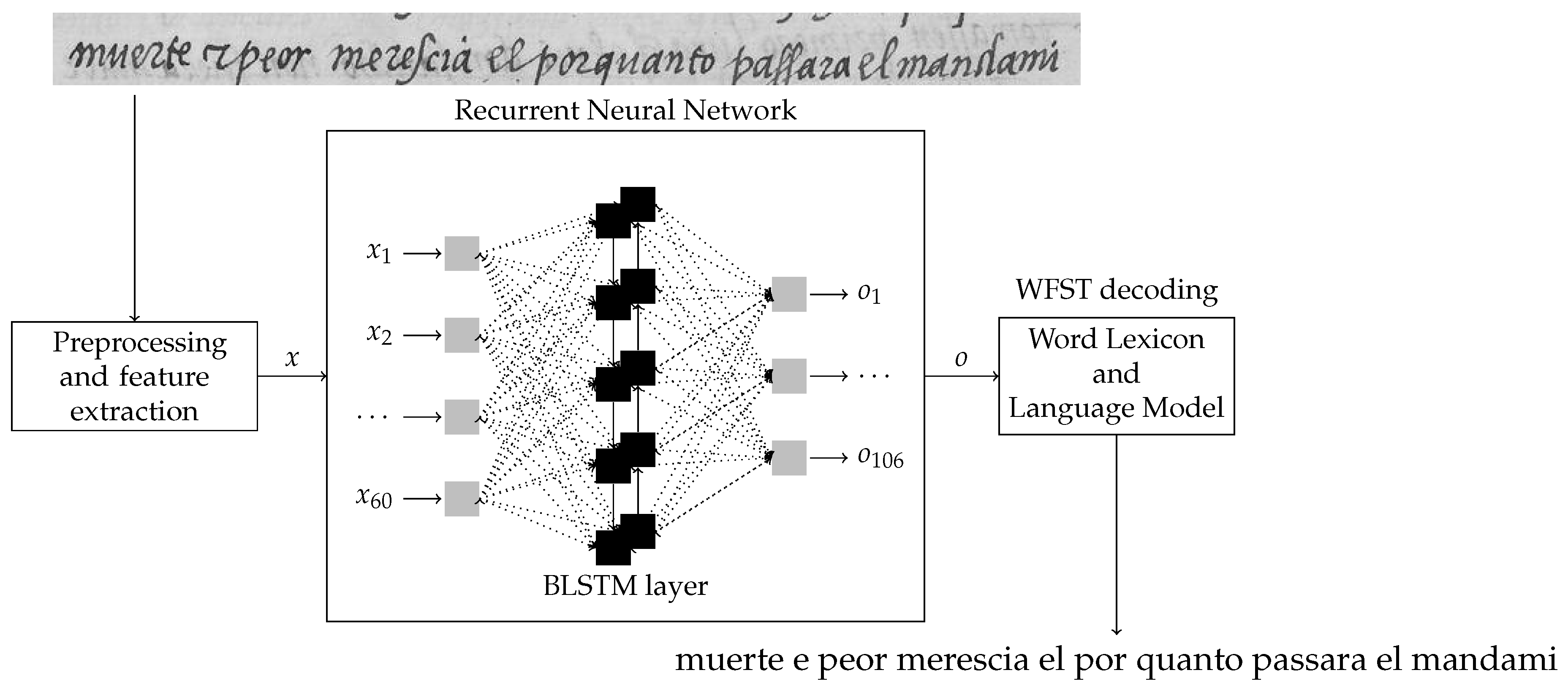
Generally, in HTR systems, the optical models are associated with dictionaries (lexical models) and Language Models (LMs), usually at the word level, in order to direct the recognition of real words and plausible word sequences (see Figure 2). In order to build open vocabulary systems, language models based on character units can be used [9]. Then, the dictionary is limited to the set of different characters, and the transition probabilities between the character models are given by a character LM. Character-based LMs are also useful for related tasks such as word spotting [10]. In the previous character LM approach or even in general word LM approaches, the optical models still model characters. However, in works such as [11,12], the optical models model strokes that are concatenated to form words.
When a word-based dictionary helps the recognition process, the handwriting recognition system can only transcribe a limited number of words. The size of the dictionary is a compromise between a too large size yielding word confusions and a too small one yielding many unknown words. Words of the test set that are not present in the HTR dictionary are denoted as Out-Of-Vocabulary (OOV) words. Several types of OOV words exist, such as common words using a less common grammatical form, misspellings, words attached to punctuation marks, hyphenated words or words containing rare characters (abbreviations, special signs, etc.).
An approach to cope with OOV words consists of extending the dictionary with external lexical resources, such as Wikipedia [13], or in the case of historical documents, with the transcription of other documents from the same period and topic [14]. From these resources, the language model can also be refined. However, in the general case, such resources may not be available, and a proportion of words (such as named entities and rare words) still remains as OOV. Another approach for coping with OOV words consists of modeling text at a sub-word level, as a sequence of characters, syllables or multi-grams [15]. Hybrid approaches [16,17] consist of using word-based language models for the most frequent words and character-based models for the less frequent ones. In sub-word approaches, the dictionary is considerably reduced to the number of lexical units, as well as the computational complexity. In addition, the language model can model unknown words by combining such lexical units.
In this work, we compare several HTR systems, based on HMMs, RNNs and convolutional RNNs (CRNNs). The CRNN is inspired from a very deep architecture presented in [18]. It consists of stacking BLSTMs and associating them with convolutional layers. Features are thus automatically extracted by the convolutional layers and processed by the BLSTM layers. We also model dictionaries and language models of our HTR systems with sub-word units. We apply this approach to the recognition of a publicly available Spanish historical documents dataset. We compare several HTR systems based on different types of sub-word units, and we show that sub-word units are more efficient than word units. We obtain, to our knowledge, the best recognition results on this Spanish dataset by associating sub-word units with the deepest HTR optical system, namely the CRNN. We also obtain high rates for the recognition of OOV words.
The rest of the paper is structured as follows: the Spanish historical manuscript used in the experimentation is presented in the next section (Section 2); the HTR systems and the experimental conditions are described in Section 3; our experiments and the obtained results are reported in Section 4; the conclusions and future work are drawn in Section 5; finally, in Appendix A, several recognition examples are shown.

2. The Rodrigo Dataset

The Rodrigo corpus [19] was obtained from the digitization of the book “Historia de España del arçobispo Don Rodrigo”, written in ancient Spanish in 1545. It is a single writer book where most pages consist of a single block of well-separated lines of calligraphical text, as the examples presented in Figure 1 and Figure 3. It is composed of 853 pages that were automatically divided into lines, giving a total number of 20,356 lines. In the standard training partition, the vocabulary size is of about 11,000 words with a set of 106 characters (the 105 different characters that appear in the text of the training partition and one extra character that appears in the text of the validation partition), including 10 numbers, 72 upper and lower case letters with and without accents, 5 punctuation marks, 1 blank space and 18 special symbols. The first 15,010 lines are publicly available on the website of the Pattern Recognition and Human Language Technology (PRHLT) research center [20]. In this work, we used this publicly available partition. The first 9000 lines were used for training the optical and language models, the next 1000 for validation and the last 5010 lines for testing.
In the Rodirgo corpus, there are many rare words and words in their archaic forms yielding a large amount of OOV words. Moreover, this corpus contains scarce OOV characters (such as: \, , , and w) that do not belong to the training set. OOV words generally include words that appear in distinct form in the training and test sets (e.g., portugal and portuḡl), abbreviations and words hyphenated differently in the training and test sets.
Table 1 presents a summary of the information contained in the partitions of the Rodrigo corpus used in this work at the three lexical units studied: words, sub-words and characters. This table presents for each lexical unit the total amount, the vocabulary size (different units), the amount of OOV units and the overlapping between the OOV contained in the validation and test partitions, i.e., the amount of OOV units contained in the test partition that are present in the validation partition.

3. Handwritten Text Recognition Systems

This section presents our proposal, the feature extraction, the models used by the implemented HTR systems and the evaluation metrics used in the experimentation.

3.1. Proposal

The HTR problem can be formulated as finding the most likely word sequence w ^ given a feature vector sequence x = ( x 1 , x 2 , , x | x | ) that represents a handwritten text line image [21], that is:
w ^ = arg max w W Pr ( w x ) = arg max w W Pr ( x w ) Pr ( w ) Pr ( x ) = arg max w W Pr ( x w ) Pr ( w )
where W represents the set of all permissible word sequences, Pr ( x ) is the probability of observing x, Pr ( w ) is the probability of the word sequence w = ( w 1 , w 2 , , w | w | ) and Pr ( x w ) is the probability of observing x by assuming that w is the underlying word sequence for x. Pr ( w ) is approximated by the Language Model (LM), whereas Pr ( x w ) is modeled by the optical model, which trains character models and concatenates them to build optical word or sub-word models.
Written words can be decomposed into small sub-word units such as characters, but they can also be decomposed into larger sub-word units such as graphemic syllables, hyphens or multigrams [15]. We choose here to compare character and hyphen word decompositions. In both cases, words are represented as a sequence of sub-word units s = ( s 1 , s 2 , , s | s | ) . Then, the HTR problem can be reformulated as finding the most likely sub-word sequence s ^ given a feature vector sequence x that represents a handwritten text image. Therefore, Equation (1) becomes:
s ^ = arg max s S Pr ( x s ) Pr ( s )
where Pr ( s ) is approximated by a sub-word LM, whereas Pr ( x s ) can be modeled by the same optical model.
It should be noted that RNN-based systems directly provide in their outputs posterior distributions of character labels, at each time step, i.e., o k t for k = 1 , , L and t = 1 , , T , T being the length of the observation sequence x and L the alphabet size. From these posteriors, the decoding can be constrained by a lexicon and a language model, in order to find the best output sequence s ^ . This can be done through Weighted Finite State Transducers (WFST) decoding (see Section 3.5), which can include several types of lexicon and language models (at word, hyphen or character levels).
Working at the sub-word level in HTR relaxes the restrictions imposed by the lexicon, allowing for a faster decoding, and given that the language model describes the relation between sub-word units, some OOV words can be decoded. Therefore, our proposal is to decode the handwritten text line images at the sub-word level and, then, from the obtained decoding output, reconstruct the words to build the final hypothesis.
First of all, the language model of sub-word units is trained using the transcription of the text lines of the training partition after a minimum preprocessing. This preprocessing consists of adding a new symbol (<SPACE>) for the separation between words and then splitting the words into sub-word sequences. In this way, the information of the separation between words is maintained.
As an example, the following text line from the training set:
Agora cuenta la historia
 
would be transformed into the following character sequence:
A g o r a~<SPACE> c u e n t a~<SPACE> l a~<SPACE> h i s t o r i a
 
or into the following sequence following the hyphenation rules for Spanish:
Ago ra <SPACE> cuen ta <SPACE> la <SPACE> his to ria
 
Then, these preprocessed transcriptions can be used to train the sub-word unit language model. Usually, n-gram language models of sub-word units are trained with a large n (large context). On the other side, the lexicon is reduced to match the list of sub-word units.
In the decoding process, the best hypothesis is processed to obtain the final hypothesis. This final process consists of collapsing the sub-word unit sequence to form words and to substitute the symbol used to mark the separation between words (<SPACE>) by a space. Figure 4 presents a text line example from the test partition whose reference transcription is:
vio e recognoscio el Astragamiento que perdiera de su gente
        
In this example, the words recognoscio and Astragamiento are OOV words. It is interesting to note their etymology. They are archaic forms from Early Modern Spanish (15th–17th century) that in Modern Spanish correspond to the forms reconoció and Estragamiento. For that reason, we could not find them in any external resource, not even in Google N-Grams [22].
The HMM decoding process with a traditional word-based approach offers the following best hypothesis:
vno & rea gustio el Astragar mando que perdona de lugar
        
which represents a Character Error Rate (CER) equal to 35.6 % with respect to the reference text-line transcription. However, using a sub-word based approach, the following best hypothesis is obtained:
vio <SPACE> & <SPACE> re ca ges cio <SPACE> el <SPACE> As tra ga mien to
<SPACE> que <SPACE> per do na <SPACE> de <SPACE> lu gar <SPACE>
      
which is transformed into the improved hypothesis (CER = 22.0 % ):
vio & recagescio el Astragamiento que perdona de lugar
  
On the other hand, with a character-based approach, the following best hypothesis is obtained:
v i o <SPACE> & <SPACE> r e c e g e s c i o <SPACE> e l <SPACE> A s t r a~g a~m i e n t o
<SPACE> q u e <SPACE> p e r d i e r a~<SPACE> d e l <SPACE> s e g u n d o
        
which results in the next final best hypothesis (CER = 17.0 % ):
vio & recegescio el Astragamiento que perdiera del segundo
        
As can be observed, the final hypotheses obtained at sub-word levels (characters, hyphenation sub-word units) in HTR are considerably better than those obtained with the word-based approach. In addition, the OOV word Astragamiento has been fully recognized. The second OOV word is recognized as recegescio or recagescio, which also improves the word-based recognition rea gustio. In Section 4, word and sub-word language modeling approaches will be compared with several types of optical HTR systems.

3.2. Handcrafted Features

Features are computed in several steps from text line images. First, the image brightness is normalized, and a median filter of size 3 × 3 pixels is applied to the entire image. Next, slant correction is performed by using the maximum variance method with a threshold of 92% [23]. Then, size normalization is performed, and the final image is scaled to a height of 40 pixels. Finally, a sequence of 60-dimensional feature vectors is extracted by a sliding window, using the method described in [24].

3.3. Lexicon and Language Models

The lexicon and language models at the sub-word level were obtained by hyphenating the vocabulary words following the rules for modern Spanish by using the testhyphens package [25] for LATEX. Lexicon models were in HTK lexicon format, where vocabulary words and sub-word units were modeled as a concatenation of symbols; however, characters were modeled as just the corresponding symbol.
Language Models (LM) were estimated as n-grams with Kneser–Ney back-off smoothing [26] by using the SRILM toolkit [27]. Different LMs were used in the experiments at word, sub-word and character levels. For the word-based system and the open-vocabulary case, the LM is trained directly from the text-line transcriptions of the training set. In the closed-vocabulary case, the LM is trained with the same transcriptions, plus the OOV words included as unigrams. For the character-based system, the closed-vocabulary case indicates that the character sequences that represent the OOV words are used for building the n-gram character LM. For both systems, word or character-based, “with validation” means that training and validation transcriptions are used for building the LM.

3.4. Optical Models

In this paper, three different approaches for optical modeling for HTR are used: traditional hidden Markov models and two deep network classifiers. The first one is based on recurrent neural networks with bi-directional long-short term memory, and the other one is based on convolutional recurrent neural networks.

3.4.1. Hidden Markov Models

The Hidden Markov Models (HMM) for optical modeling were trained with HTK [28]. The trained models are left-to-right character models including four states. The observation probabilities in each state are described by a mixture distribution of 64 Gaussians. The number of character models is 106, and words and sub-words are modeled by the concatenation of compound character HMMs. The HMM system uses as input sequences of handcrafted features. HMM HTR systems were implemented by using the iATROS recognizer [29].

3.4.2. Deep Models Based on BLSTMs

In this approach, we use an RNN to estimate the posterior probabilities of the characters at the frame level (features vector). Therefore, the size of the input layer corresponds to the size of the handcrafted feature vectors and the size of the output layer to the number of different characters. The frame-level labeling required to train this neural network was generated from a forced alignment decoding by a previously trained HMM recognition system [30]. This forced alignment decoding and the model training were repeated several times until the convergence of the assignment of the frame labels to the optical model.
Then, as presented in Figure 5, our RNN is formed by 60 neurones at the input layer, 500 BLSTM neurones at the hidden layer with a hyperbolic tangent activation function and 106 neurones at the output layer with a softmax function. The training was performed by using RNNLIB [31], and the main parameters (such as the size of the hidden layer) were tuned by using the validation partition. The Weighted Finite State Transducers (WFST) decoding (see Section 3.5) can be designed to output word, sub-word or character sequences. For each output type, the lexicon and language model have to be modified accordingly, and no additional modification is necessary in the system.

3.4.3. Deep Models Based on Convolutional Recurrent Neural Networks

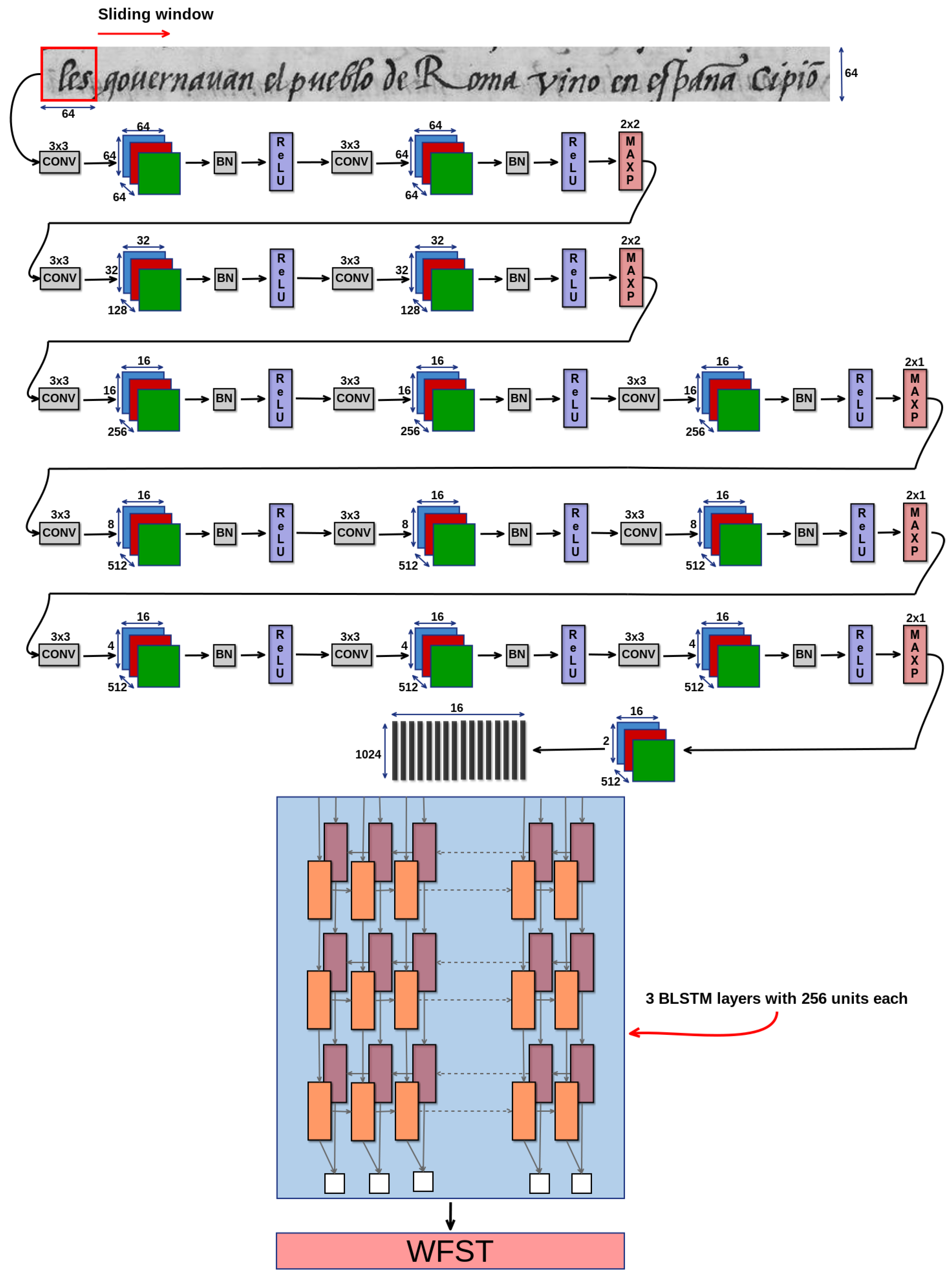
The Convolutional Recurrent Neural Network (CRNN) [32] is inspired by the VGG16 architecture [33] that was developed for image recognition. We use a stack of 13 convolutional (3 × 3 filters, 1 × 1 stride) layers followed by three bi-directional LSTM layers with 256 units per layer (see Figure 6). Each LSTM unit has one cell with enabled peephole connections. Spatial pooling (max) is employed after some convolutional layers. To introduce non-linearity, the Rectified Linear Unit (ReLU) activation function was used after each convolution. It has the advantage of being resistant to the vanishing gradient problem while being simple in terms of computation and was shown to work better than sigmoid and hyperbolic tangent activation functions [34]. A square-shaped sliding window is used to scan the text-line image in the direction of the writing. The height of the window is equal to the height of the text-line image, which has been normalized to 64 pixels. The window overlap is equal to two pixels to allow continuous transition of the convolution filters. For each analysis window of 64 × 64 pixels in size, 16 feature vectors are extracted from the feature maps produced by the last convolutional layer and fed into the observation sequence. For each of the 16 columns of the last 512 feature maps, the columns of a height of two pixels are concatenated into a feature vector of size 1024 (512 × 2). Thanks to the CTCtranscription layer [35], the system is end-to-end trainable. The convolutional filters and the LSTM units weights are thus jointly learned using the back-propagation procedure. We combined the forward and backward outputs at the end of the BLSTM stack [36] rather than after each BLSTM layer, in order to decrease the number of parameters. We also chose not to add additional fully-connected layers since, by adding such layers, the network had more parameters, converged more slowly and performed worse. Hyper parameters such as the number of convolution layers and the number of BLSTM layers were set up on a validation set. The LSTM unit weights were initialized as per the method of [37], which proved to work well and helps the network to converge faster. This allows the network to maintain a constant variance across the network layers, which keeps the signal from exploding to a high value or vanishing to zero. The weight matrices were initialized with a uniform distribution.
The Adam optimizer [38] was used to train the network with the initial learning rate of 0.001. This algorithm could be thought of as an upgrade for RMSProp [39], offering bias correction and momentum [40]. It provides adaptive learning rates for the stochastic gradient descent update computed from the first and second moments of the gradients. It also stores an exponentially decaying average of the past squared gradients (similar to Adadelta [41] and RMSprop) and the past gradients (similar to momentum). Batch normalization, as described in [42], was added after each convolutional layer in order to accelerate the training process. It basically works by normalizing each batch by both the mean and variance. The network was trained in an end-to-end fashion with the CTC loss function [35].

3.5. Decoding with Deep Optical Models

Decoding for both deep net systems was performed with Weighted Finite State Transducers (WFST). Our decoder is based on the CTC-specific implementation proposed by [43] for speech recognition. A “token” WFST was designed to handle all possible label sequences at the frame level, so as to allow for the occurrence of the blank label along with the repetition of non-blank labels. It can map a sequence of frame-level CTC labels to a single character. A search graph is built with three WFSTs (T, L and G) compiled independently and combined as follows:
S = T min ( det ( L G ) )
T, L and G are the token, lexicon and grammar WFSTs respectively, whereas ∘, det and min denote composition, determination and minimization, respectively. The determination and minimization operations are needed to compress the search space, yielding a faster decoding.

3.6. Evaluation Metrics

The quality of the obtained transcriptions was assessed using the edit distance [44] with respect to the reference text, at the word and at the character level. The Word Error Rate (WER) is this edit distance at the word level and can be calculated as the minimum number of substitutions, deletions and insertions needed to transform the transcription into the reference, divided by the number of words of the reference:
WER = s + d + i n · 100
where s is the number of substitutions, d the number of deletions, i the number of insertions and n the total number of words in the reference.
Similarly, this edit distance can be calculated at the character level, giving the Character Error Rate (CER). In this framework, the CER value is especially interesting, since transcription errors are usually corrected at the character level. The OOV Word Accuracy Rate (OOV WAR) was measured as the amount of recognized OOV words over the total amount of OOV words. The statistical significance of experimental results can be estimated by means of confidence intervals. Generally, when comparing two experimental results, it is always true that if the confidence intervals do not overlap, we can say that the difference is statistically significant [45]. In this work, confidence intervals of probability 95% ( α = 0.025 ) were calculated by using the bootstrapping method with 10,000 repetitions [46] for these rate measures.
Finally, as language models are probability distributions over entire sentences or texts, perplexity [47] can be used to evaluate their performance over a reference text. In this work, we use the perplexity presented by a character LM over the OOV words (as sequences of characters), to assess the differences between the recognized and unrecognized OOV words.

4. Experimental Results

In the test experiments, we compared the performance on the test partition of the Rodrigo corpus. Different systems were compared, the first one based on HMMs, the second one based on RNN and the third one on CRNN. For the three systems, experiments were performed at word, sub-word, and character levels. We first explore the influence of the size of the LM context (n-gram degree). Then, we develop an analysis of the difference between the structure of recognized and unrecognized OOV words. The last experiment compares the results obtained in three different cases: open vocabulary, closed vocabulary and when using the validation samples for training the LM.
We observed that in the training partition of Rodrigo, usually there are no spaces between words and punctuation marks, so we decided to remove those spaces from the hypotheses offered by the word-based systems. Therefore, in the word-based cases, the recognized OOV words correspond to words attached to punctuation marks, which were correctly recognized after removing the space between them (see Figure A2).

4.1. Study of the Context Size Influence

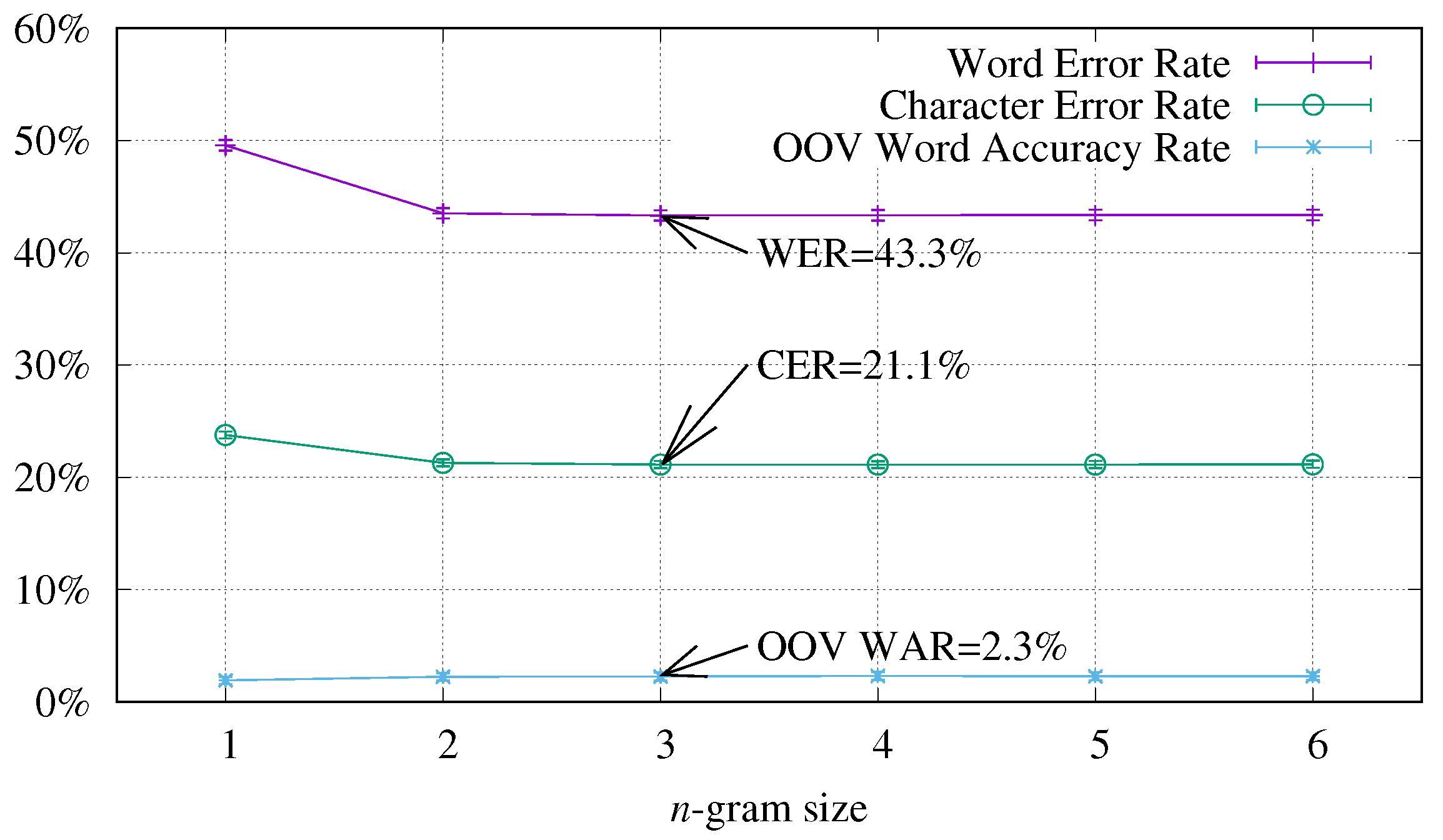
Figure 7 presents the results obtained for the word-based HMM system (in terms of WER and CER) by using n-gram LM with different context sizes n = { 1 , , 6 } . As can be observed in this figure, the best result was obtained by using a three-gram LM; concretely, a WER equal to 43.3 % ± 0.5 , a CER equal to 21.1 % ± 0.3 and an OOV WAR equal to 2.3 % ± 0.4 .
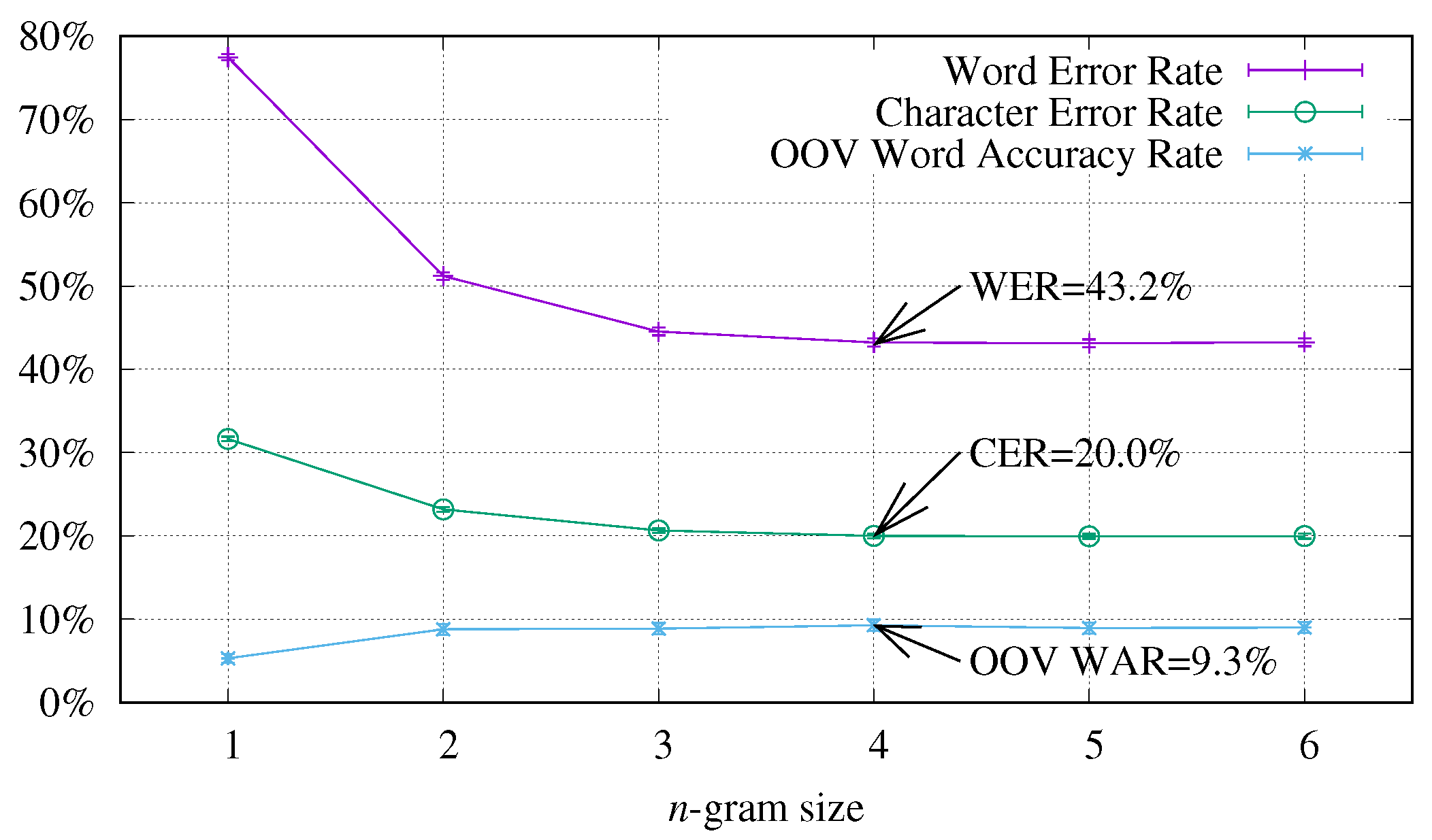
Then, the performance of the HMM system at the sub-word level was tested. Figure 8 presents the results obtained using sub-word n-gram LM with different sizes n = { 1 , , 6 } in terms of WER, CER and recognition accuracy of the OOV words. The best result was obtained with a sub-word language model of size n = 4 (a WER equal to 43.2 % ± 0.5 and a CER equal to 20.0 % ± 0.3 ). Regarding the recognition of OOV words, the sub-word approach was able to recognize correctly 9.3 % ± 0.7 of the OOV words.
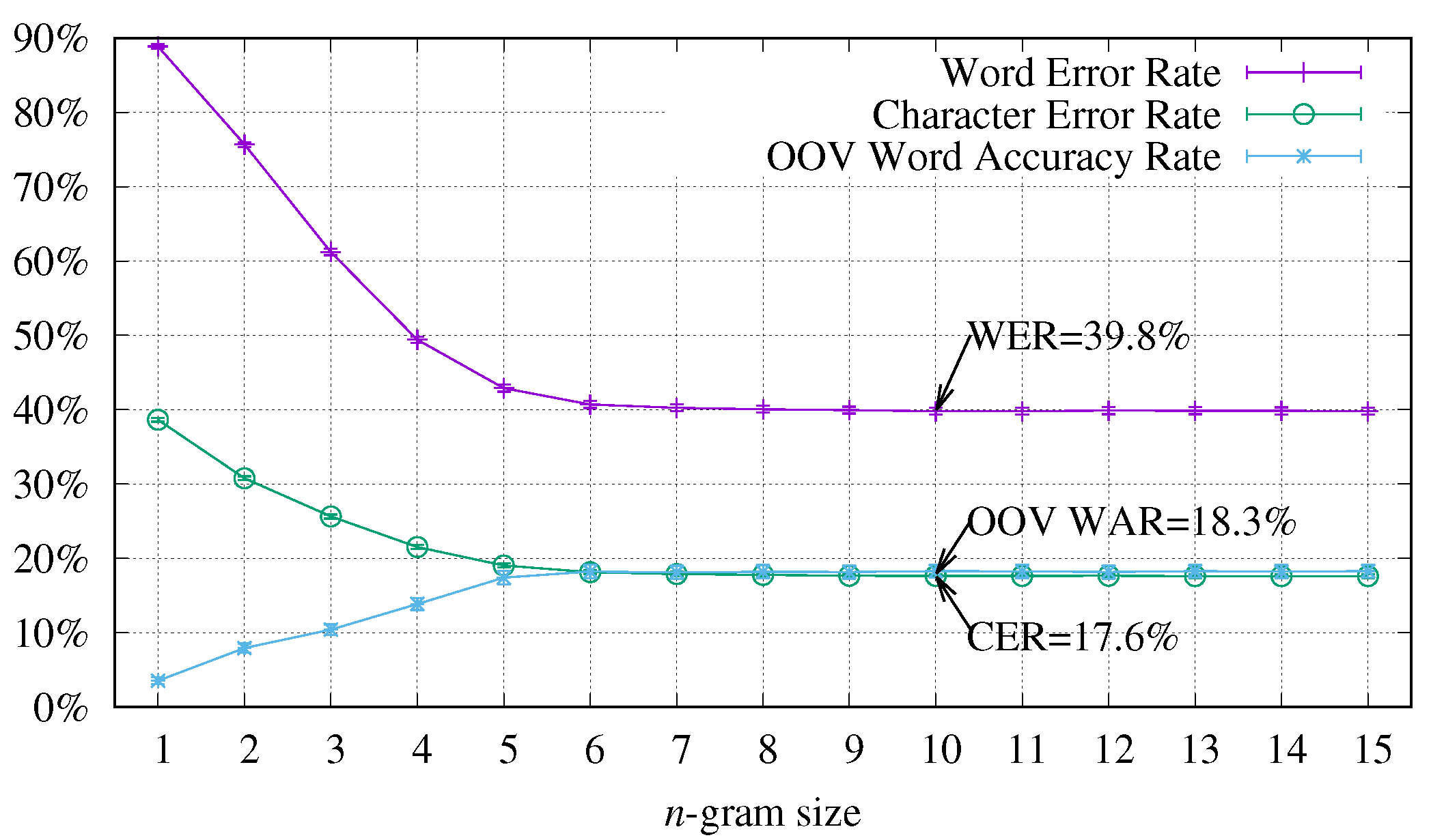
Figure 9 presents the results obtained for the HMM system using character n-gram LM with different degrees n = { 1 , , 15 } in terms of WER, CER and recognition accuracy of the OOV words. Although similar results are obtained for n 6 , the overall best result was obtained with a character language model of degree n = 10 (a WER equal to 39.8 % ± 0.5 and a CER equal to 17.6 % ± 0.3 ). Regarding the recognition of OOV words, this character-based approach was able to recognize correctly 18.3 % ± 0.9 of the OOV words using no external resource or dictionary, but a character language model only.
Table 2 presents a summary of the obtained best results for the test experiments for the HMM system. As can be observed, the improvement offered by the sub-word approach is not statistically significant at the WER level compared to the results obtained from the word-based system. Nevertheless, the character-based approach offers 9.3 % of statistically-significant relative improvement over the baseline in terms of WER and 17.0 % of statistically-significant relative improvement over the baseline in terms of CER. Thus, using a dictionary and LM at the word level performs worse than using a single character-based n-gram LM, with n large enough. This demonstrates the interest in working at the character level for transcribing historical manuscripts. We study in the following the structure of the OOV words in comparison with the training words (Section 4.2). We also study the effect of reducing the OOV rate, either by using the validation set or by closing the vocabulary (Section 4.3).

4.2. Study of the Relation between the Structure of the OOV Words and the Training Words

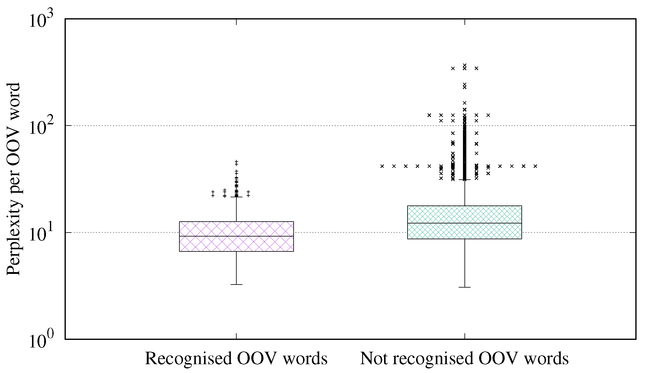
The character-based approach is able to recognize some OOV words given that the character-based LM learns the structure of the words contained in the training set. In order to verify this hypothesis, we measured the perplexity presented by the best character-based LM (10-gram) for decoding each one of the 4918 OOV words as their corresponding character sequences. Figure 10 presents the obtained perplexity per OOV word separated into two distributions, recognized and unrecognized OOV words. Table 3 summarizes the main features of these distributions. As expected, the recognized OOV words present lower perplexity than the unrecognized OOV words. The overlap of both distributions makes us think that there is still room for improvement given that more OOV words could be recognized.

4.3. Study of the Effect of Closing the Vocabulary and Adding the Transcription of the Validation Set for Training the LM

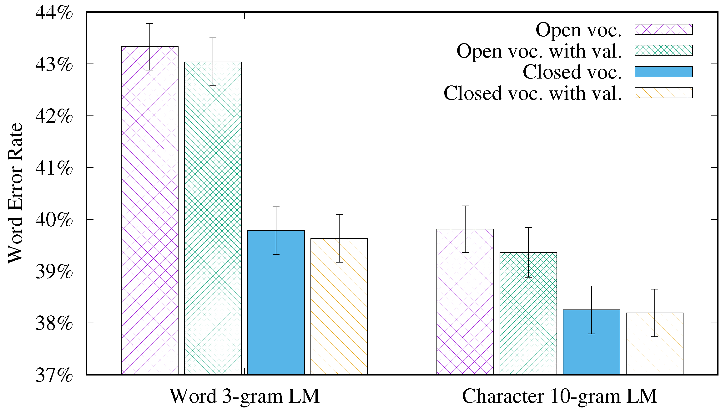
After the adjustment of the decoding parameters with the validation set, the transcription of the text lines contained in this partition can be used to train an improved LM that, hopefully, will reduce the amount of OOV words. Moreover, the OOV words can be included in the vocabulary as unigrams (closed vocabulary experiments) to verify their influence on the recognition. These conditions were experimented for the best language models at word and character levels (3-gram for the word based system and 10-gram for the character-based system). Given that the sub-word approach presented no significative difference in terms of WER, compared to the word-based system (see Table 2), this approach was not tested in this experiment.
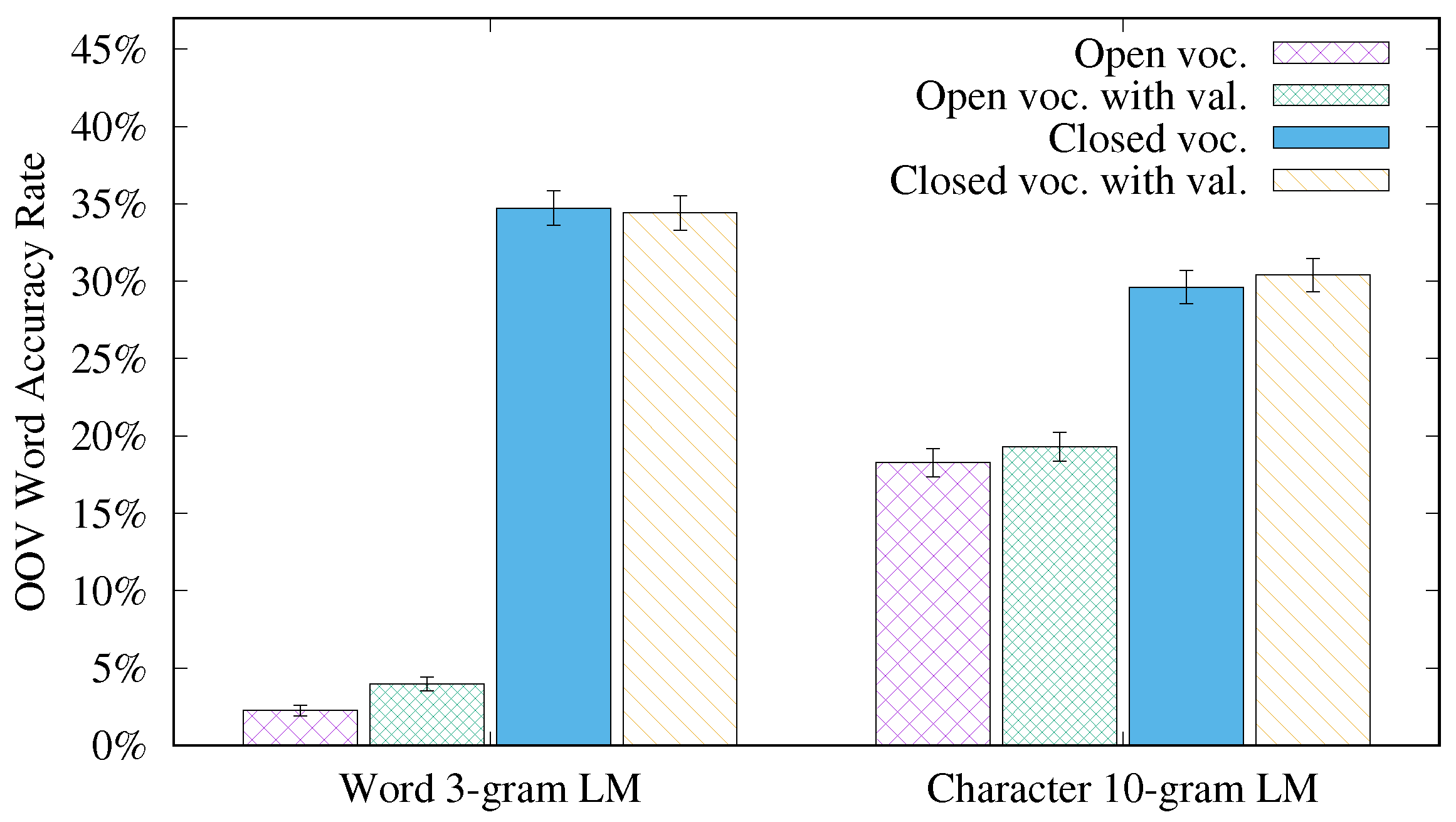
Figure 11, Figure 12 and Figure 13 allow comparing the obtained results for the word-based system and the character-based approach with open and closed vocabulary, with and without the use of the validation samples when training the LM (see Section 3.4). On the one hand, as can be seen in Figure 11 and Figure 13, the use of the validation set does not significantly improve the word-based recognition in terms of WER or CER. However, this additional information is very useful in the character-based approach. As can be observed in Figure 11, a statistically-significant improvement in terms of CER is achieved ( 16.9 % ± 0.3 instead of 17.6 % ± 0.3 ). This improvement allows increasing the OOV word recognition accuracy (see Figure 12). On the other side, although closing the vocabulary significantly improves the recognition performance, it is interesting to note the beneficial effect of the use of the validation samples in the character-based approach. It is also interesting to note in Figure 11 and Figure 13 that the character-based system, even in the more difficult case (“open-vocabulary”), outperforms, in terms of CER, the word-based system in the best case (“closed-vocabulary”). In the closed vocabulary conditions, the word-based system recognizes more OOV words than the character-based system, 34.7 % ± 1.2 instead of 29.6 % ± 1.1 (see Figure 12). However, in the real-world case, i.e., the open-vocabulary conditions, the character-based system performs better.

4.4. Study of the Context Size Influence Using Deep Optical Models

This last part of the experimentation studies the influence of the different language units and the context size of the language model, on the HTR system based on deep neural networks (see Section 3.4.2 and Section 3.4.3).

4.4.1. Results for Deep Models Based on Recurrent Neural Networks with BLSTMs

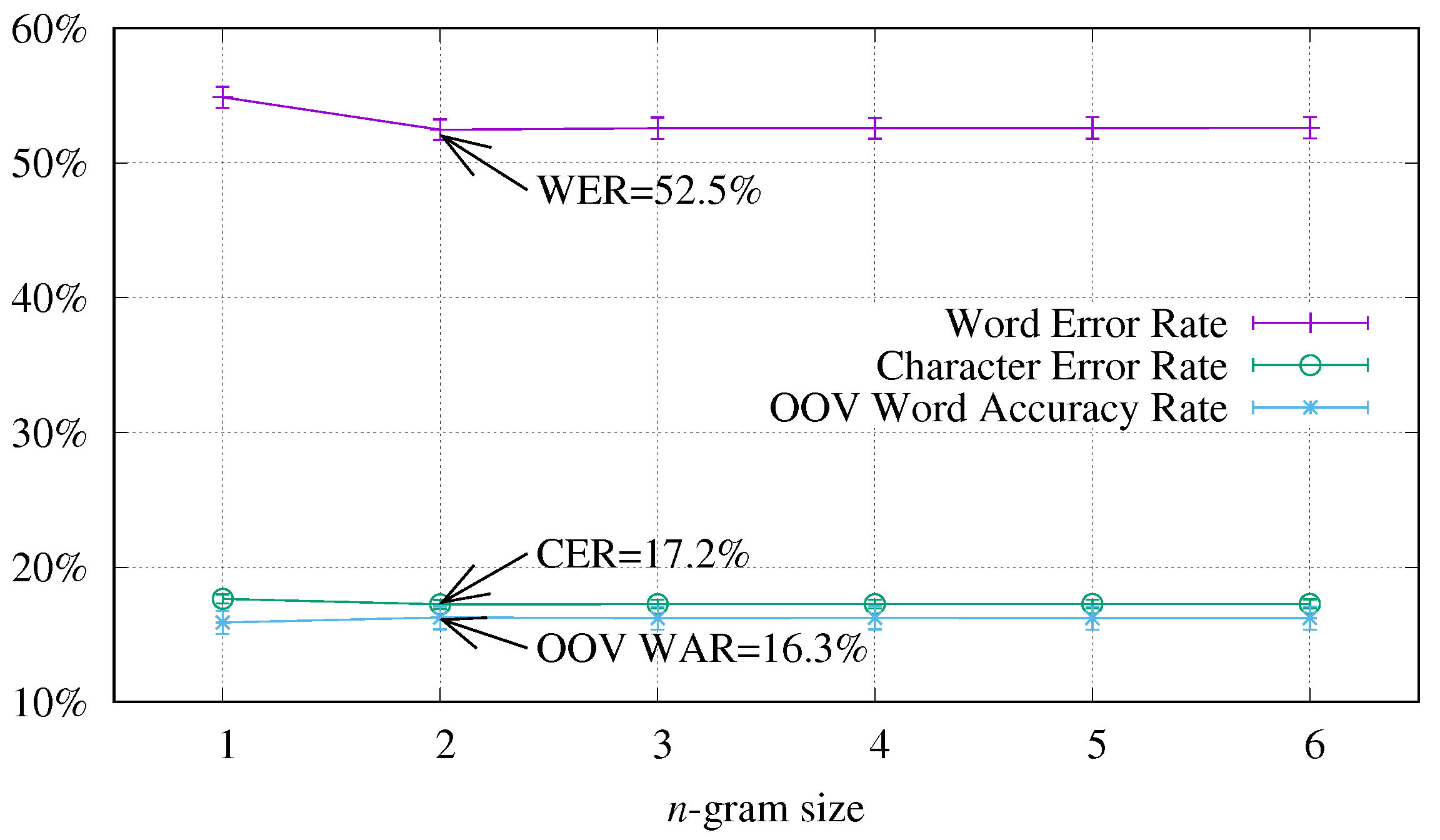
In Figure 14, the recognition results obtained for the word-based RNN system are presented. As explained before, in this case, the recognized OOV words correspond to words attached to punctuation marks, which were correctly recognized after removing the space between them (see the example presented in Figure A2). Compared with the word-based HMM system, the obtained results are significantly worse in terms of WER; however, in terms of CER and OOV word recognition accuracy, the obtained results are significantly better. Concretely, the best result was obtained by using a two-gram LM, and it presents a WER equal to 52.5 % ± 0.8 , a CER equal to 17.2 % ± 0.3 and an OOV WAR equal to 16.3 % ± 0.9 .
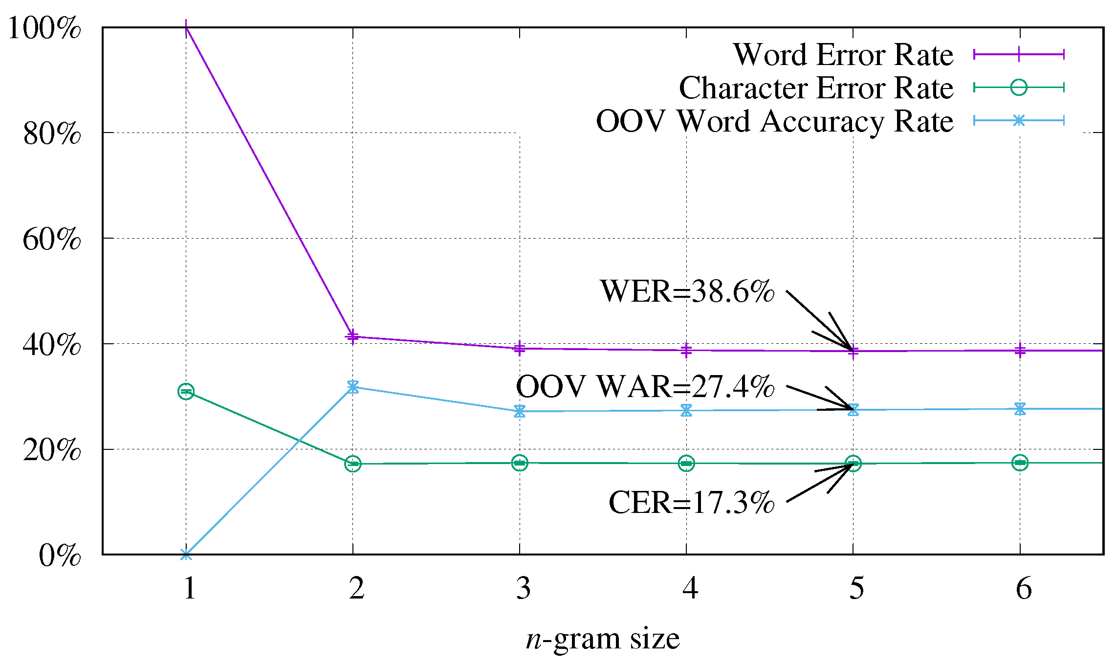
Figure 15 shows the results obtained using sub-word n-gram LM. As can be observed, the WFST approach has no context information about the separation between words when sub-word unigrams LM are used; therefore, it is unable to reconstruct words correctly in spite of obtaining a good CER. We will see this effect in the next experiments with the sub-word and character-based deep net systems. In this case, the best result was obtained with a five-gram language model (a WER equal to 38.6 % ± 0.5 , a CER equal to 17.3 % ± 0.3 and an OOV WAR equal to 27.4 % ± 1.1 ).
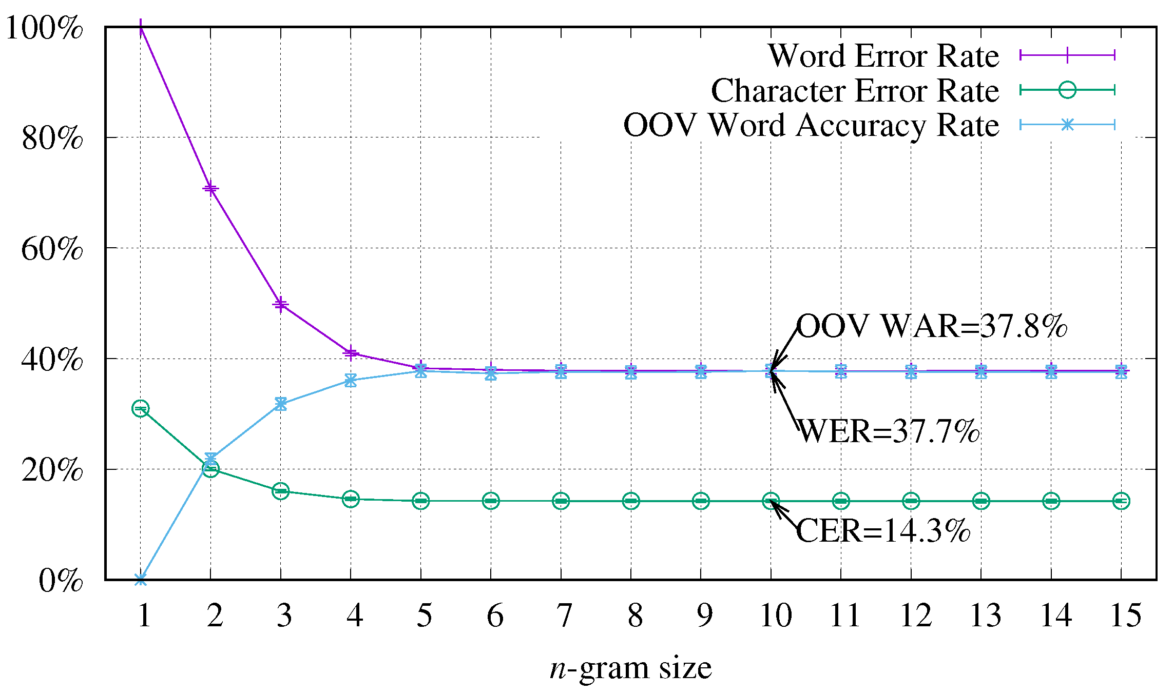
The results obtained with the RNN system using character n-gram LM are presented in Figure 16. As in the character-based HMM experiments, similar results are obtained for n 6 , and the overall best result was obtained with a 10-gram character language model: a WER equal to 37.7 % ± 0.5 , a CER equal to 14.3 % ± 0.3 and an OOV WAR equal to 37.8 % ± 1.1 .
A summary of the obtained best results for the test experiments for the RNN system is presented in Table 4. As can be observed, generally, the RNN approach performs better than the traditional HMM approach. Although the use of the word-based RNN system obtains a statistically-significant relative deterioration of 19.6 % over the HMM system ( 43.9 % ± 0.5 ) in terms of WER, 18.9 % statistically-significant relative improvement in terms of CER ( 21.2 % ± 0.3 ) can be considered. Moreover, 16.3 % of OOV words, which correspond to words followed by punctuation marks, are well recognized.
The use of sub-word units offers better results than using words, allowing one to obtain significant improvements in terms of WER and CER over the HMM system. In this case, the use of a five-gram LM trained with hyphenated words allowed obtaining statistically-significant improvements at the WER level over the use of a two-gram LM of full words. However, as for the HMM system, the overall best results are obtained by using the character-based approach: a WER equal to 37.7 % ± 0.5 , a CER equal to 14.3 % ± 0.3 and an OOV WAR equal to 37.8 % ± 1.1 .

4.4.2. Results for Deep Models Based on Convolutional Recurrent Neural Networks

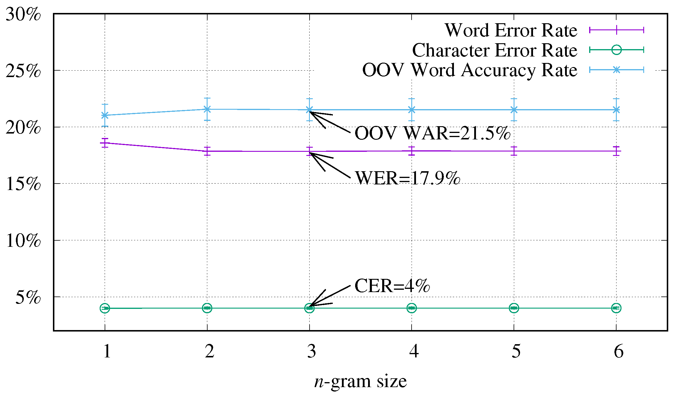
Figure 17 presents the recognition results obtained for the word-based CRNN system. As in the previous word-based systems, the recognized OOV words correspond to words attached to punctuation marks, which were correctly recognized after removing the space between them (see the example presented in Figure A2). The best result, obtained by using a three-gram LM, presents a WER equal to 17.9 % ± 0.4 , a CER equal to 4.0 % ± 0.1 and an OOV WAR equal to 21.5 % ± 1.0 .
The results obtained using sub-word n-gram LM are shown in Figure 18. The best result was obtained with a four-gram language model (a WER equal to 14.8 % ± 0.3 and a CER equal to 3.4 % ± 0.1 ). Regarding the recognition of OOV words, the sub-word approach allowed correctly recognizing 42.4 % ± 1.5 of the OOV words.
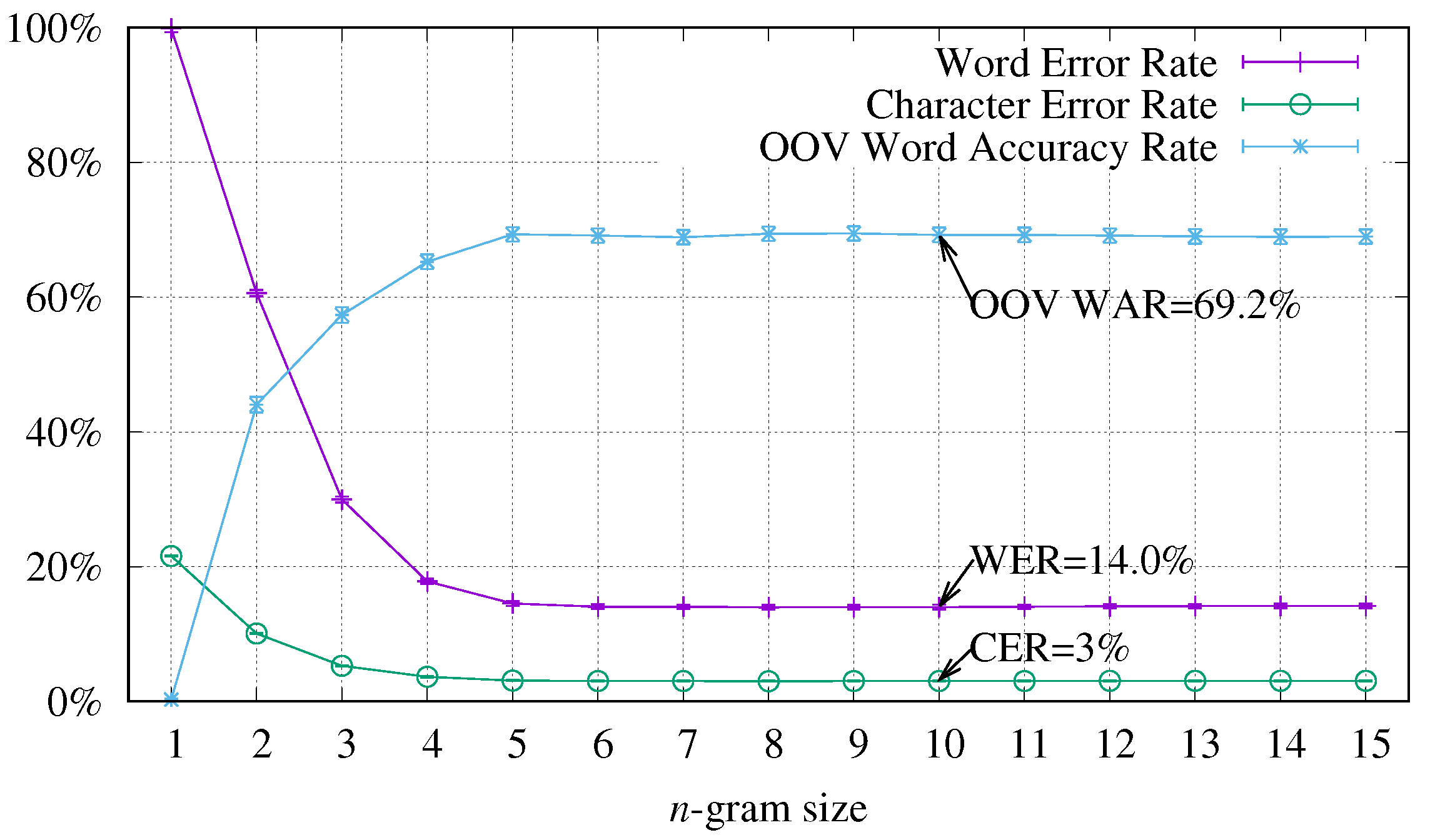
Figure 19 presents the results obtained with the CRNN system using character n-gram LM. As in the previous character-based experiments, similar results are obtained for n 6 , and the overall best result was obtained with a 10-gram character language model (a WER equal to 14.0 % ± 0.3 and a CER equal to 3.0 % ± 0.1 ). Regarding the recognition of OOV words, this approach was able to recognize correctly 69.2 % ± 1.1 of the OOV words using no external resource or dictionary, but a character language model only.
Table 5 presents a summary of the obtained best results for the test experiments for the CRNN system. As can be observed, the use of deep optical models allows one to obtain a statistically-significant relative improvement of 59.2 % over the HMM system ( 43.9 % ± 0.5 ) in terms of WER and 81.1 % statistically-significant relative improvement over the HMM system in terms of CER. Regarding OOV words, 21.5 % of OOV words, which correspond to words followed by punctuation marks, are well recognized. It should be noted that these results are also significantly better than those obtained by the HMM system in the closed vocabulary experiments (Figure 11, Figure 12 and Figure 13).
The use of sub-word units performs better than using words. In this case, the use of a four-gram LM trained with hyphenated words allowed obtaining statistically-significant improvements over the use of a three-gram LM of full words. However, the overall best results are obtained by using the character-based approach: a WER equal to 14.0 % ± 0.3 , a CER equal to 3.0 % ± 0.1 and an OOV WAR equal to 69.2 % ± 1.1 . These results confirm the interest of working at the character level for transcribing historical manuscripts.

5. Conclusions

In this paper, we deal with the transcription of historical documents, for which no external linguistic resources are available. We have developed various HTR systems that model language at word and sub-lexical levels. We have shown that character-based language modeling performs best.
The strengths of the proposed work are:
  • comparing several types of HTR systems (HMM-based, RNN-based).
  • proposing a state-of-the-art HTR system for the transcription of ancient Spanish documents whose optical part is based on very deep nets (CRNNs).
  • proposing to associate the optical HTR system with a dictionary and a language model based on sub-lexical units. These units are shown to be efficient in order to cope with OOV words.
  • reaching with such optical and LM HTR components the best overall recognition results on a publicly available Spanish historical dataset of document images.
In future work, we would like to extend this work using other kinds of language models, such as models based on RNN.

Acknowledgments

Work partially supported by projects READ: Recognition and Enrichment of Archival Documents - 674943 (European Union’s H2020) and CoMUN-HaT: Context, Multimodality and User Collaboration in Handwritten Text Processing - TIN2015-70924-C2-1-R (MINECO/FEDER), and a DGA-MRIS (Direction Générale de l’Armement - Mission pour la Recherche et l’Innovation Scientifique) scholarship.

Author Contributions

Emilio Granell and Edgard Chammas conceived and implemented the recognition systems (HMM, BLSTM, CRNN). All authors contributed in equal proportion to the design of the research and to the final manuscript.

Conflicts of Interest

The authors declare no conflict of interest.

Appendix A. Some Recognition Examples
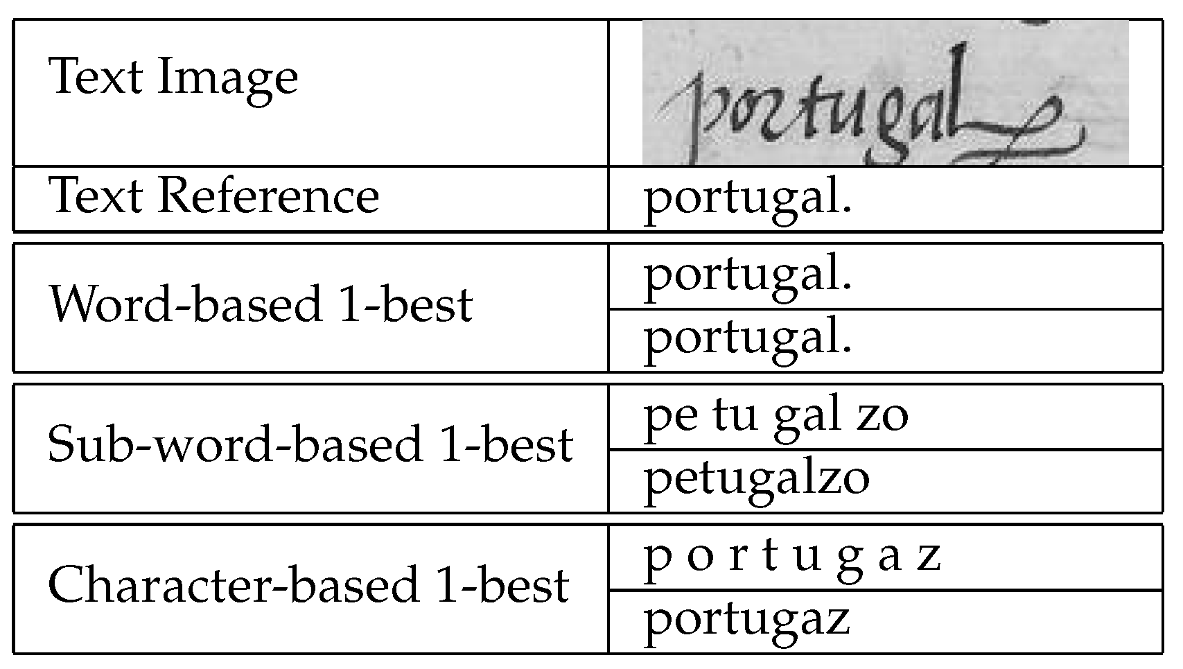
This Appendix presents some recognition examples. Figure A1, Figure A2 and Figure A3 present the best hypothesis obtained for several lines of the Rodrigo corpus in the open vocabulary experiments, by using a 3-gram word-based LM, a 4-gram sub-word-based LM and a 10-gram character-based LM.
Figure A1. Example of the best hypotheses obtained for the 12th line of page 500 of Rodrigo.
Jimaging 04 00015 g0a1
Figure A2. Example of the best hypotheses obtained for the 9th line of page 619 of Rodrigo.
Jimaging 04 00015 g0a2
Figure A3. Example of the best hypotheses obtained for the 4th line of page 514 of Rodrigo.
Jimaging 04 00015 g0a3

References

  1. España-Boquera, S.; Castro-Bleda, M.J.; Gorbe-Moya, J.; Zamora-Martinez, F. Improving Offline Handwritten Text Recognition with Hybrid HMM/ANN Models. IEEE Trans. Pattern Anal. Mach. Intell. 2011, 33, 767–779. [Google Scholar] [CrossRef] [PubMed]
  2. Al-Hajj-Mohamad, R.; Likforman-Sulem, L.; Mokbel, C. Combining Slanted-Frame Classifiers for Improved HMM-Based Arabic Handwriting Recognition. IEEE Trans. Pattern Anal. Mach. Intell. 2009, 31, 1165–1177. [Google Scholar] [CrossRef] [PubMed]
  3. Vinciarelli, A. A survey on off-line cursive word recognition. Pattern Recognit. 2002, 35, 1433–1446. [Google Scholar] [CrossRef]
  4. Bianne-Bernard, A.L.; Menasri, F.; El-Hajj, R.; Mokbel, C.; Kermorvant, C.; Likforman-Sulem, L. Dynamic and Contextual Information in HMM modeling for Handwritten Word Recognition. IEEE Trans. Pattern Anal. Mach. Intell. 2011, 99, 2066–2080. [Google Scholar] [CrossRef] [PubMed]
  5. Graves, A. Supervised Sequence Labelling with Recurrent Neural Networks. Ph.D. Thesis, Technische Universität München, Munich, Germany, 2008. [Google Scholar]
  6. Xie, Z.; Sun, Z.; Jin, L.; Feng, Z.; Zhang, S. Fully convolutional recurrent network for handwritten Chinese text recognition. In Proceedings of the 23rd International Conference on Pattern Recognition (ICPR), Cancun, Mexico, 4–8 December 2016; pp. 4011–4016. [Google Scholar]
  7. Bluche, T.; Messina, R. Gated Convolutional Recurrent Neural Networks for Multilingual Handwriting Recognition. In Proceedings of the 13th International Conference on Document Analysis and Recognition (ICDAR), Kyoto, Japan, 13–15 November 2017. [Google Scholar]
  8. Sudholt, S.; Fink, G.A. PHOCNet: A deep convolutional neural network for word spotting in handwritten documents. In Proceedings of the 15th International Conference on Frontiers in Handwriting Recognition (ICFHR), Shenzhen, China, 23–26 October 2016; pp. 277–282. [Google Scholar]
  9. Brakensiek, A.; Rottland, J.; Kosmala, A.; Rigoll, G. Off-line handwriting recognition using various hybrid modeling techniques and character n-grams. In Proceedings of the 7th International Workshop on Frontiers in Handwritten Recognition, Amsterdam, The Netherlands, 11–13 September 2000; pp. 343–352. [Google Scholar]
  10. Fischer, A.; Frinken, V.; Bunke, H.; Suen, C.Y. Improving hmm-based keyword spotting with character language models. In Proceedings of the 12th International Conference on Document Analysis and Recognition (ICDAR), Washington, DC, USA, 25–28 August 2013; pp. 506–510. [Google Scholar]
  11. Santoro, A.; Parziale, A.; Marcelli, A. A Human in the Loop Approach to Historical Handwritten Documents Transcription. In Proceedings of the 15th International Conference on Frontiers in Handwriting Recognition (ICFHR), Shenzhen, China, 23–26 October 2016; pp. 222–227. [Google Scholar]
  12. Stefano, C.D.; Marcelli, A.; Parziale, A.; Senatore, R. Reading Cursive Handwriting. In Proceedings of the 12th International Conference on Frontiers in Handwriting Recognition, Kolkata, India, 16–18 November 2010; pp. 95–100. [Google Scholar]
  13. Oprean, C.; Likforman-Sulem, L.; Popescu, A.; Mokbel, C. Handwritten word recognition using Web resources and recurrent neural networks. Int. J. Doc. Anal. Recognit. (IJDAR) 2015, 18, 287–301. [Google Scholar] [CrossRef]
  14. Frinken, V.; Fischer, A.; Martínez-Hinarejos, C.D. Handwriting recognition in historical documents using very large vocabularies. In Proceedings of the 2nd International Workshop on Historical Document Imaging and Processing, Washington, DC, USA, 24 August 2013; pp. 67–72. [Google Scholar]
  15. Swaileh, W.; Paquet, T. Handwriting Recognition with Multi-gram language models. In Proceedings of the 14h International Conference on Document Analysis and Recognition (ICDAR), Kyoto, Japan, 10–15 November 2017. [Google Scholar]
  16. Kozielski, M.; Rybach, D.; Hahn, S.; Schlüter, R.; Ney, H. Open vocabulary handwriting recognition using combined word-level and character-level language models. In Proceedings of the 2013 International Conference on Acoustics, Speech and Signal Processing (ICASSP ’13), Vancouver, BC, Canada, 26–31 May 2013; pp. 8257–8261. [Google Scholar]
  17. Messina, R.; Kermorvant, C. Over-generative finite state transducer n-gram for out-of-vocabulary word recognition. In Proceedings of the 11th IAPR International Workshop on Document Analysis Systems (DAS), Tours, France, 7–10 April 2014; pp. 212–216. [Google Scholar]
  18. Shi, B.; Bai, X.; Yao, C. An end-to-end trainable neural network for image-based sequence recognition and its application to scene text recognition. IEEE Trans. Pattern Anal. Mach. Intell. 2017, 39, 2298–2304. [Google Scholar] [CrossRef] [PubMed]
  19. Serrano, N.; Castro, F.; Juan, A. The RODRIGO Database. In Proceedings of the 7th International Conference on Language Resources and Evaluation (LREC), Valletta, Malta, 17–23 May 2010; pp. 2709–2712. [Google Scholar]
  20. Pattern Recognition and Human Language Technology (PRHLT) Research Center. 2018. Available online: https://www.prhlt.upv.es (accessed on 5 January 2018).
  21. Fischer, A. Handwriting Recognition in Historical Documents. Ph.D. Thesis, University of Bern, Bern, Switzerland, 2012. [Google Scholar]
  22. Michel, J.B.; Shen, Y.K.; Aiden, A.P.; Veres, A.; Gray, M.K.; Brockman, W.; Team, T.G.B.; Pickett, J.P.; Hoiberg, D.; Clancy, D.; et al. Quantitative analysis of culture using millions of digitized books. Science 2010, 331, 176–182. [Google Scholar] [CrossRef] [PubMed] [Green Version]
  23. Pastor, M.; Toselli, A.H.; Vidal, E. Projection profile based algorithm for slant removal. In Lecture Notes in Computer Science, Proceedings of the International Conference on Image Analysis and Recognition (ICIAR’04), Porto, Portugal, 29 September–1 October 2004; Springer: Berlin, Germany, 2004; Volume 3212, pp. 183–190. [Google Scholar]
  24. Toselli, A.H.; Juan, A.; González, J.; Salvador, I.; Vidal, E.; Casacuberta, F.; Keysers, D.; Ney, H. Integrated Handwriting Recognition and Interpretation using Finite-State Models. Int. J. Pattern Recognit. Artif. Intell. 2004, 18, 519–539. [Google Scholar] [CrossRef]
  25. Testhyphens – Testing hyphenation patterns. 2018. Available online: https://www.ctan.org/tex-archive/macros/latex/contrib/testhyphens (accessed on 5 January 2018).
  26. Kneser, R.; Ney, H. Improved backing-off for M-gram language modeling. In Proceedings of the 1995 International Conference on Acoustics, Speech, and Signal Processing (ICASSP’95), Detroit, MI, USA, 9–12 May 1995; Volume 1, pp. 181–184. [Google Scholar]
  27. Stolcke, A. SRILM—An extensible language modeling toolkit. In Proceedings of the 3rd Interspeech, Denver, CO, USA, 16–20 September 2002; pp. 901–904. [Google Scholar]
  28. Young, S.; Evermann, G.; Gales, M.; Hain, T.; Kershaw, D.; Liu, X.; Moore, G.; Odell, J.; Ollason, D.; Povey, D.; et al. The HTK Book (for HTK Version 3.4); Cambridge University Engineering Department: Cambridge, UK, 2006. [Google Scholar]
  29. Luján-Mares, M.; Tamarit, V.; Alabau, V.; Martínez-Hinarejos, C.D.; Pastor, M.; Sanchis, A.; Toselli, A.H. iATROS: A Speech and Handwriting Recognition System. V Jornadas en Tecnologías del Habla. 2008, pp. 75–78. Available online: http://citeseerx.ist.psu.edu/viewdoc/download?doi=10.1.1.329.6708&rep=rep1&type=pdf (accessed on 5 January 2018).
  30. Hermansky, H.; Ellis, D.P.W.; Sharma, S. Tandem connectionist feature extraction for conventional HMM systems. In Proceedings of the 2000 IEEE International Conference on Acoustics, Speech, and Signal Processing (ICASSP’00), Istanbul, Turkey, 5–9 June 2000; Volume 3, pp. 1635–1638. [Google Scholar]
  31. Graves, A. RNNLIB: A Recurrent Neural Network Library for Sequence Learning Problems. 2016. Available online: http://sourceforge.net/projects/rnnl/ (accessed on 5 January 2018).
  32. Chammas, E. Structuring Hidden Information in Markov Modeling with Application to Handwriting Recognition. Ph.D. Thesis, Telecom ParisTech, Paris, France, 2017. [Google Scholar]
  33. Simonyan, K.; Zisserman, A. Very deep convolutional networks for large-scale image recognition. arXiv, 2014; arXiv:1409.1556. [Google Scholar]
  34. Gu, J.; Wang, Z.; Kuen, J.; Ma, L.; Shahroudy, A.; Shuai, B.; Liu, T.; Wang, X.; Wang, G. Recent advances in convolutional neural networks. arXiv, 2015; arXiv:1512.07108. [Google Scholar]
  35. Graves, A.; Fernández, S.; Gomez, F.; Schmidhuber, J. Connectionist temporal classification: labeling unsegmented sequence data with recurrent neural networks. In Proceedings of the 23rd international conference on Machine learning ACM, Pittsburgh, PA, USA, 25–29 June 2006; pp. 369–376. [Google Scholar]
  36. Zeyer, A.; Schlüter, R.; Ney, H. Towards Online-Recognition with Deep Bidirectional LSTM Acoustic Models. In Proceedings of the 2016 INTERSPEECH, San Francisco, CA, USA, 8–12 September 2016; pp. 3424–3428. [Google Scholar]
  37. Glorot, X.; Bengio, Y. Understanding the difficulty of training deep feedforward neural networks. In Proceedings of the Thirteenth International Conference on Artificial Intelligence and Statistics, Sardinia, Italy, 13–15 May 2010; pp. 249–256. [Google Scholar]
  38. Kingma, D.; Ba, J. Adam: A method for stochastic optimization. arXiv, 2014; arXiv:1412.6980. [Google Scholar]
  39. Tieleman, T.; Hinton, G. Lecture 6.5-rmsprop: Divide the gradient by a running average of its recent magnitude. COURSERA Neural Netw. Mach. Learn. 2012, 4, 26–31. [Google Scholar]
  40. Qian, N. On the momentum term in gradient descent learning algorithms. Neural Netw. 1999, 12, 145–151. [Google Scholar] [CrossRef]
  41. Zeiler, M.D. ADADELTA: an adaptive learning rate method. arXiv, 2012; arXiv:1212.5701. [Google Scholar]
  42. Ioffe, S.; Szegedy, C. Batch normalization: Accelerating deep network training by reducing internal covariate shift. In Proceedings of the International Conference on Machine Learning, Lille, France, 6–11 July 2015; pp. 448–456. [Google Scholar]
  43. Miao, Y.; Gowayyed, M.; Metze, F. EESEN: End-to-end speech recognition using deep RNN models and WFST-based decoding. In Proceedings of the 2015 IEEE Workshop on Automatic Speech Recognition and Understanding (ASRU), Scottsdale, AZ, USA, 13–17 December 2015; pp. 167–174. [Google Scholar]
  44. Levenshtein, V.I. Binary codes capable of correcting deletions, insertions, and reversals. Sov. Phys. Dokl. 1966, 10, 707–710. [Google Scholar]
  45. Knezevic, A. Overlapping Confidence Intervals and Statistical Significance; StatNews; Cornell University Statistical Consulting Unit: Ithaca, NY, USA, 2008; Volume 73. [Google Scholar]
  46. Bisani, M.; Ney, H. Bootstrap estimates for confidence intervals in ASR performance evaluation. In Proceedings of the IEEE International Conference on Acoustics, Speech, and Signal Processing ICASSP’04, Montreal, QC, Canada, 17–21 May 2004; Volume 1, pp. 409–412. [Google Scholar]
  47. Brown, P.F.; Della Pietra, V.J.; Mercer, R.L.; Della Pietra, S.A.; Lai, J.C. An Estimate of an Upper Bound for the Entropy of English. Comput. Linguist. 1992, 18, 31–40. [Google Scholar]
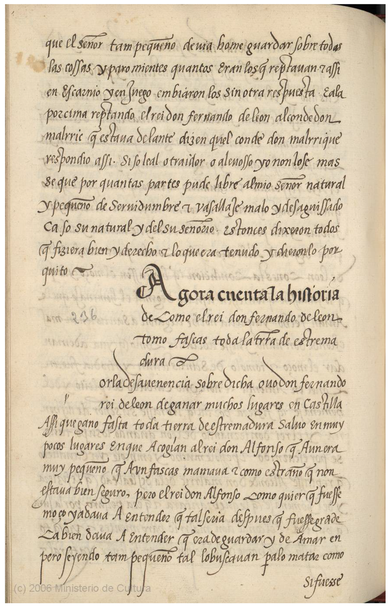
Figure 1. Sample image of a Spanish document from the 16th century.
Jimaging 04 00015 g001
Figure 2. Scheme of a handwritten text recognition system.
Jimaging 04 00015 g002
Figure 3. Page 515 of the Rodrigo dataset.
Jimaging 04 00015 g003
Figure 4. Text line sample. “Recognoscio” and “Astragamiento” are rare words; recognoscio is an archaic form of reconoció and Astragamiento an ancient form of Estragamiento.
Jimaging 04 00015 g004
Figure 5. Bi-directional Long-Short Term Memory (BLSTM) system architecture. The BLSTM RNN outputs posterior distributions o at each time step. The decoding is performed with Weighted Finite State Transducers (WFST) using a lexicon and a language model at word level.
Jimaging 04 00015 g005
Figure 6. CRNN system architecture.
Jimaging 04 00015 g006
Figure 7. Results obtained by the HMM word-based system using n-gram language models with size n = { 1 , , 6 } .
Jimaging 04 00015 g007
Figure 8. Results obtained by decoding at the HMM sub-word level by using n-gram language models with size n = { 1 , , 6 } .
Jimaging 04 00015 g008
Figure 9. Results obtained by decoding at the HMM character level by using n-gram language models with size n = { 1 , , 15 } .
Jimaging 04 00015 g009
Figure 10. Distribution of the perplexity presented by the 10-gram character Language Model (LM) per recognized and unrecognized OOV words (decomposed into character sequences) by the HMM system.
Jimaging 04 00015 g010
Figure 11. CER results obtained by the best word-based HMM system and the best character-based HMM system with open and closed vocabulary, with and without using the validation samples for training the LM.
Jimaging 04 00015 g011
Figure 12. Recognition accuracy rate for OOV words by the best word-based HMM system and the best character-based HMM system with open and closed vocabulary, with and without using the validation samples for training the LM.
Jimaging 04 00015 g012
Figure 13. WER results obtained by the best word-based HMM system and the best character-based HMM system with open and closed vocabulary, with and without using the validation samples for training the LM.
Jimaging 04 00015 g013
Figure 14. Results obtained by the RNN word-based system using n-gram language models.
Jimaging 04 00015 g014
Figure 15. Results obtained by the RNN sub-word-based system using n-gram language models.
Jimaging 04 00015 g015
Figure 16. Results obtained by the RNN character-based system using n-gram language models.
Jimaging 04 00015 g016
Figure 17. Results obtained by the CRNN word-based system using n-gram language models with size n = { 1 , , 6 } .
Jimaging 04 00015 g017
Figure 18. Results obtained by the CRNN sub-word-based system using n-gram language models with size n = { 1 , , 6 } .
Jimaging 04 00015 g018
Figure 19. Results obtained by the CRNN character-based system using n-gram language models with size n = { 1 , , 15 } .
Jimaging 04 00015 g019
Table 1. Description of the partitions of the Rodrigo corpus used in this work.
PartitionLinesWords
Total/Diff./OOV (over.)
Sub-Words
Total/Diff./OOV (over.)
Characters
Total/Diff./OOV (over.)
Training900098,232/12,650/-148,070/3045/-493,126/105/-
Validation100010,899/3016/85014,907/1074/754,936/82/1
Test501055,195/7453/4918 (203)73,660/1418/55 (11)272,132/91/14 (1)
Table 2. Overall best results on the Rodrigo test set in terms of WER, CER and OOV WAR for the HMM system.
MeasureWord
3-gram
Sub-Word
4-gram
Character
10-gram
WER 43.9 % ± 0.5 43.2 % ± 0.5 39.8 % ± 0.5
CER 21.2 % ± 0.3 20.0 % ± 0.3 17.6 % ± 0.3
OOV WAR 2.3 % ± 0.3 9.3 % ± 0.7 18.3 % ± 0.9
Table 3. Features of the perplexity per OOV word recognized and unrecognized distributions for the HMM character-based 10-gram LM. Q1, Q2 and Q3 are respectively the 1th, 2nd and 3rd quartile, IQR the interquartile range, Min. and Max. the minimum and maximum values and SD the standard deviation.
DistributionQ1Q2Q3IQRMin.Max.SD
Recognized6.649.2212.575.943.2646.055.37
Unrecognized8.7012.2117.759.053.06367.0716.25
Table 4. Summary of the best results in terms of WER, CER and OOV WAR for the RNN system.
MeasureWord
2-gram
Sub-Word
5-gram
Character
10-gram
WER 52.5 % ± 0.8 38.6 % ± 0.5 37.7 % ± 0.5
CER 17.2 % ± 0.3 17.3 % ± 0.3 14.3 % ± 0.3
OOV WAR 16.3 % ± 0.9 27.4 % ± 1.1 37.8 % ± 1.1
Table 5. Overall best results on the Rodrigo test set in terms of WER, CER and OOV WAR for the CRNN system.
MeasureWord
3-gram
Sub-Word
4-gram
Character
10-gram
WER 17.9 % ± 0.4 14.8 % ± 0.3 14.0 % ± 0.3
CER 4.0 % ± 0.1 3.4 % ± 0.1 3.0 % ± 0.1
OOV WAR 21.5 % ± 1.0 42.4 % ± 1.5 69.2 % ± 1.1