GPU Acceleration of the Most Apparent Distortion Image Quality Assessment Algorithm

Abstract

The primary function of multimedia systems is to seamlessly transform and display content to users while maintaining the perception of acceptable quality. For images and videos, perceptual quality assessment algorithms play an important role in determining what is acceptable quality and what is unacceptable from a human visual perspective. As modern image quality assessment (IQA) algorithms gain widespread adoption, it is important to achieve a balance between their computational efficiency and their quality prediction accuracy. One way to improve computational performance to meet real-time constraints is to use simplistic models of visual perception, but such an approach has a serious drawback in terms of poor-quality predictions and limited robustness to changing distortions and viewing conditions. In this paper, we investigate the advantages and potential bottlenecks of implementing a best-in-class IQA algorithm, Most Apparent Distortion, on graphics processing units (GPUs). Our results suggest that an understanding of the GPU and CPU architectures, combined with detailed knowledge of the IQA algorithm, can lead to non-trivial speedups without compromising prediction accuracy. A single-GPU and a multi-GPU implementation showed a 24× and a 33× speedup, respectively, over the baseline CPU implementation. A bottleneck analysis revealed the kernels with the highest runtimes, and a microarchitectural analysis illustrated the underlying reasons for the high runtimes of these kernels. Programs written with optimizations such as blocking that map well to CPU memory hierarchies do not map well to the GPU’s memory hierarchy. While compute unified device architecture (CUDA) is convenient to use and is powerful in facilitating general purpose GPU (GPGPU) programming, knowledge of how a program interacts with the underlying hardware is essential for understanding performance bottlenecks and resolving them.

1. Introduction

Images and videos undergo several transformations from capture to display in various formats. The key to transferring these contents over networks lies in the design of image/video analysis and processing algorithms that can simultaneously tackle two opposing goals: (1) The ability to handle potentially massive content sizes (e.g., 8 K video); while (2) achieving the results in a timely fashion (e.g., near real time) on practical computing hardware. One such analysis application is the field of image and video quality assessment (QA), which deals with automated techniques of scoring the quality of images/videos in a manner that is in agreement with the quality perceived by a human consumer. Perceptual QA algorithms fill a critical role in determining what is acceptable quality and what is unacceptable from a human visual perspective. Indeed, such algorithms have proved useful for the design and evaluation of many applications (e.g., [1,2,3,4,5]).

Over the last decade, the field of image and video QA has seen enormous growth in research activity, particularly in the design of new QA algorithms for improved quality predictions, with particular growth over the last five years (see, e.g., [1,2,3,4,5,6,7,8]; see also [9] for a recent review). However, an equally important, though much less pursued topic of QA research is in regards to computational performance. Many existing QA algorithms have been designed from the outset to sacrifice or even completely neglect the use of perceptual models in order to achieve runtime practicality (e.g., [1,10,11,12,13] all use fast, but perceptually inaccurate multiscale decompositions); whereas other algorithms forgo runtime practicality to achieve higher perceptual accuracy (e.g., [14,15]). Thus, an urgent and crucial task for QA research is to investigate ways of achieving practical runtimes without sacrificing the prediction accuracy and robustness afforded by proper perceptual modeling.

One method of achieving large performance gains would be to implement the algorithms on a graphics processing unit (GPU). Using GPUs for general-purpose computational tasks (termed GPGPU) leverages the parallelism of GPUs with programing models, such as CUDA and open computing language (OpenCL). Generally, the types of problems that are well-suited for a GPU implementation are ones which can be decomposed into an algorithmic form that exposes a large amount of data-level parallelism. Furthermore, if a specific computational problem can be decomposed into an algorithmic structure that exposes both data- and task-level parallelism, then multiple GPUs can be used to gain even greater performance benefits.

The use of the GPU for acceleration of general image/video analysis and processing has emerged as a recent thrust for attaining fast results without sacrificing accuracy on traditionally time- and/or memory-prohibitive applications. For example, for image-domain-warping [16], Wang et al. investigated the use of the GPU as a solution for achieving real-time results on the otherwise extremely intensive task of view synthesis. For video encoding, Momcilovic et al. [17] present not only GPU acceleration, but multi-GPU acceleration on a heterogeneous system, with a speedup of 8.5× over a multi-core CPU version. Zhang et al. describe GPU acceleration using CUDA for 3D full-body motion tracking in real time [18]. The main research challenge in these and related applications is how to research and design efficient data-level parallelism strategies: What parts to offload to the GPU, what parts to keep on the CPU, and how to minimize data transfer between the two. As the size of multimedia content continues to grow at an astounding rate, researchers and practitioners must be aware of parallelism and data-transfer strategies, and ideally apply this knowledge during the algorithm-design stages. To this end, in this paper, we address the issue of GPU acceleration of the perceptual and statistical processing stages used in QA, in the hopes to inform the design, implementation, and deployment of future multimedia QA systems.

Perceptual QA algorithms, in particular, should be prime candidates for a GPU implementation due to the fact that their underlying models attempt to mimic arrays of visual neurons, which also operate in a massively parallel fashion. Furthermore, many perceptual models employ multiple independent stages, which are candidates for task-level parallelization. However, as demonstrated in previous studies [19,20,21,22], the need to transfer data to and from the GPU’s dynamic random-access memory (DRAM) gives rise to performance degradation due to memory bandwidth bottlenecks. This memory bandwidth bottleneck is commonly the single largest limiting factor in the use of GPUs for image and video processing applications. The specific impacts of this bottleneck on a GPU/multi-GPU implementation of a perceptual QA algorithm has yet to be investigated.

To address this issue, in this paper, we implement and analyze the Most Apparent Distortion (MAD) [14] image QA (IQA) algorithm, which is highly representative of a modern perceptual IQA algorithm that can potentially gain massive computational performance improvements using GPUs. MAD has consistently been reported to be among the very best full-reference IQA algorithms in terms of prediction accuracy (see, e.g., [23]). Furthermore, the underlying perceptual models used in MAD have been used for other applications such as for video QA [24] and for digital watermarking [25]. However, MAD employs relatively extensive perceptual modeling which imposes a large runtime that prohibits its widespread adoption into real-time applications. MAD exhibits both levels of parallelism which potentially allows for large performance gains from a multi-GPU implementation.

Here, we analyze the potential performance gains and bottlenecks between single- and multiple-GPU implementations of MAD using Nvidia’s Compute Unified Device Architecture (CUDA; Nvidia Corporation, Santa Clara, CA, USA). As we will demonstrate, it is possible for the perceptual modeling to achieve near-real-time performance using a single-GPU CUDA implementation that parallelizes the modeled neural responses and neural interactions, in a manner not unlike the parallel structure of the primary visual cortex. We further demonstrate that by using three GPUs, and by placing the task-parallel sections of the algorithm on separate GPUs, an even larger performance gain can be realized, though care must be taken to mask the latency in inter-GPU and GPU-CPU memory transfers (see [26,27] for related masking strategies).

In our previous related work [28], we compared the timings of naive vs. optimized C++ ports of MAD, and vs. using a Matlab-based GPU implementation of only the log-Gabor decomposition. Although significant speedups were obtained relative to the naive implementation, the use of the GPU contributed only a 1.6×–1.8× speedup over the CPU-based optimizations, which is reasonable considering only the log-Gabor decomposition was deployed on the GPU, and considering the fact that it was a Matlab-based GPU port. Later, in [22], for CPU-only implementations of six QA algorithms (including MAD), a hotspot analysis was performed to identify sections of code that were performance bottlenecks, and a microarchitectural analysis was performed to identify the underlying causes of these bottlenecks. In the current manuscript, the key novelties compared to our prior work are as follows: (1) we implemented all of MAD in CUDA, thereby allowing analyses of all of the stages (detection, appearance, memory transfers); (2) we tested three different GPUs to examine the effects of different GPU architectures; (3) we further analyzed the differences between using a single GPU vs. parallelizing MAD across three GPUs (multi-GPU implementation) to investigate how the results scale with the number of GPUs; and (4) finally, we performed a microarchitectural analysis of the key bottleneck kernel (the CUDA kernel which computes the various local statistics) to gain insight into and inform future implementations about the GPU memory infrastructure usage.

The main contributions of this work are as follows. First, we demonstrate how to map highly representative perceptual models (from MAD, but used in many IQA algorithms) onto different GPU architectures. The main research challenge for this task is to properly and timely allocate different threads to accomplish different paralleled image processing steps within an algorithm, while simultaneously considering the various bottlenecks due to memory transfers. Second, we identify and analyze the bottlenecks by using both the CUDA profiler and a microarchitectural analysis. Based on this investigation, we propose some software and hardware solutions that can potentially alleviate the bottlenecks that allow the algorithm to run in near real time. For example, it is common to observe irregular memory accesses on the GPU arising from an exorbitant number of transactions and global memory accesses to the off-chip DRAM. Via our microarchitectural analysis, we identify the CUDA kernel with the largest bottleneck, and we propose the use of a shared memory feature provided by the NVIDIA GPU to resolve the bottleneck and improve performance. Finally, we provide a similar mapping strategy and preliminary investigation of the perceptual models on a multi-GPU setting. We run the same CUDA code on three different NVIDIA GPUs (Titan Black, Tesla K40 and GTX 960). It can be observed that the runtime of the algorithm is greatly reduced even though the number of memory transfers across the GPUs has increased.

This paper is organized as follows: Section 2 provides a brief review of related work on efforts to accelerate IQA algorithms and/or its underlying computations. Section 3 provides an overview of MAD and details of its original implementation. In Section 4, we provide details of our CUDA implementation of MAD. In Section 5, we present a performance analysis of the implementation tested on various GPUs. General conclusions are provided in Section 6.

2. Related Work

Current approaches to accelerate IQA algorithms often follow two main trends. One is a software-based approach, which focuses on optimizing the algorithm itself to improve computational efficiency. The other is a hardware-based approach, which often employs more performant programming languages (e.g., changing from Java to C/C++) and more powerful computing architectures (e.g., porting a CPU implementation to GPU implementation). In addition, some acceleration approaches employ both trends to achieve additional gains in speed. In this section, we provide a brief review of current approaches for accelerating QA algorithms. We also provide brief reviews of GPU-based approaches to accelerate some typical image-processing-related techniques that can potentially accelerate QA algorithms.

2.1. Acceleration of QA Algorithms

Acceleration of QA algorithms has been proposed via software-based approaches, hardware-based approaches, and combinations thereof. The software-based approach implements the QA algorithm by using more efficient analyses, often by approximating the most time-consuming stages. As a result, the final quality estimate may be different from the original. In contrast, the hardware-based approach most often capitalizes on the prevalence of data- or task-independent, possibly repeated computations which have the potential to be run in parallel. Thus, the acceleration can be accomplished without changing the final quality estimate.

In [29], Xu et al. proposed a novel fast FSIM [30] algorithm (FFSIM), which accelerates FSIM by replacing the computationally expensive phase congruency measure with Weber contrast to obtain the visual salience similarity and weighting coefficients for quality estimation. A multiscale version of the FFSIM algorithm (MS-FFSIM) is also proposed, which better mimics the spatial frequency response characteristics of the human visual system.

In [31], Chen et al. presented the fast SSIM [11] and fast MS-SSIM [32] algorithms, which accelerate the original algorithms by using three strategies: (1) an integral image [33] technique is employed to compute the luminance similarity; (2) the Roberts gradient templates are used to compute the contrast and structure terms; and (3) the Gaussian weighting window used for computing the contrast and structure terms was replaced by an integer approximation. For fast MS-SSIM, a further algorithm-level modification that skips the contrast and structure terms at the finest scale was proposed. Fast SSIM and fast MS-SSIM were shown to be, respectively, 2.7× and 10× faster than the original counterparts.

In [27], Okarma et al. presented a GPGPU technique for accelerating their combined video quality algorithm (a video quality assessment algorithm developed by Okarma using SSIM, MS-SSIM, and VIF [34]). In this work, a CUDA-based implementation was described to compute SSIM and MS-SSIM in a parallelized fashion. To overcome CUDA’s memory bandwidth limitations, the computed quality estimates for each image fragment were stored in GPU registers and transferred only once to the system memory. Consequently, 150× and 35× speedup of SSIM and MS-SSIM were observed.

In [28], Phan et al. proposed four techniques to accelerate the MAD IQA algorithm: (1) using integral images for the local statistical computation; (2) using procedural expansion and strength reduction; (3) using a GPGPU implementation of the log-Gabor decomposition; and (4) precomputation and caching of the log-Gabor filters. As reported in [22], the first two modifications yielded an approximate 17× speedup over the original MAD implementation, and the latter two yield an approximately 47× speedup. However, it is important to note that these speedups were relative to a naive, unoptimized C++ implementation of MAD that required nearly one minute to execute. The use of the GPU added only a 1.6×–1.8× speedup over the CPU-based optimizations. Later, in [22], for CPU-only implementations of six QA algorithms (including MAD), a hotspot analysis was performed to identify sections of code that were performance bottlenecks, and a microarchitectural analysis was performed to identify the underlying causes for these bottlenecks.

It is also worth mentioning that in recent years there have been numerous QA algorithms which operate based on deep-learning, where the training and testing is most commonly performed on the GPU (see, e.g., [35,36,37,38,39,40,41,42]), particularly for no-reference/blind QA. Such deep-learning models are performed on the GPU, primarily to accelerate the training, and therefore these approaches can be quite fast after training. The main objective is model development, with speed being an added benefit. This is a different objective from our current paper, which is to examine how common perceptual-based models (contrast sensitivity filter, log-Gabor filterbank, local statistical comparisons, etc.) used in MAD may benefit from single- and multiple-GPU implementations, and how these implementations interact with the memory infrastructure.

2.2. GPU-based Acceleration on Other Image-Processing-Related Techniques

In the context of general image processing, some of the underlying analyses performed during IQA have also been independently accelerated. Such analyses are often well-suited for acceleration via the GPU owing to the prevalence of computations that are repeated over pixels/coefficients (e.g., 2D convolutions, transforms, morphological operations). Most research been focused on accelerating various 2D transforms, such as the Fourier transform [43,44,45], discrete cosine transform [1,46,47,48], discrete wavelet transform [49,50,51], and Gabor transform [52]. Because most IQA algorithms employ these types of image decompositions, acceleration of these image transforms can theoretically benefit many IQA algorithms.

The GPU has also been employed to accelerate neural networks, which can be used for general image analysis, and can thus benefit IQA (e.g., [53]). For example, detailed descriptions of implementing neural networks on the GPU have been presented in [54,55]. In [56], the GPU was used to accelerate a deep-learning network for an image recognition task. In [57], the GPU was used for accelerating the restricted Boltzmann machine. In [58], a parallel model of the self-organizing-map neural network applied to the Euclidean traveling sales-man problem was implemented on GPU platform. In [59], two parallel training approaches (multithreaded CPU and CUDA) for backpropagation neural networks were developed and analyzed for face recognition.

In summary, the GPU has become a prevalent and increasingly important platform for IQA-related acceleration. In the following section, we describe our approach for GPU-based acceleration of the MAD IQA algorithm. As we will demonstrate, by capitalizing on MAD’s data- and task-independent properties, our CUDA implementation can achieve near-real-time QA while simultaneously yielding quality predictions that are numerically equivalent to the original implementation.

3. Description of the MAD Algorithm

As mentioned in Section 2, MAD is a full-reference IQA algorithm which models two distinct perceptual strategies: QA based on visual detection, and QA based on visual appearance. In this subsection, we describe the various stages of MAD in terms of: (1) the objective(s) of each stage; (2) how the objective(s) are estimated via signal-processing-based analyses; (3) and how the analyses were implemented in Matlab/C++. The goal of this description is to provide a background and context for later comparison with the CUDA implementation.

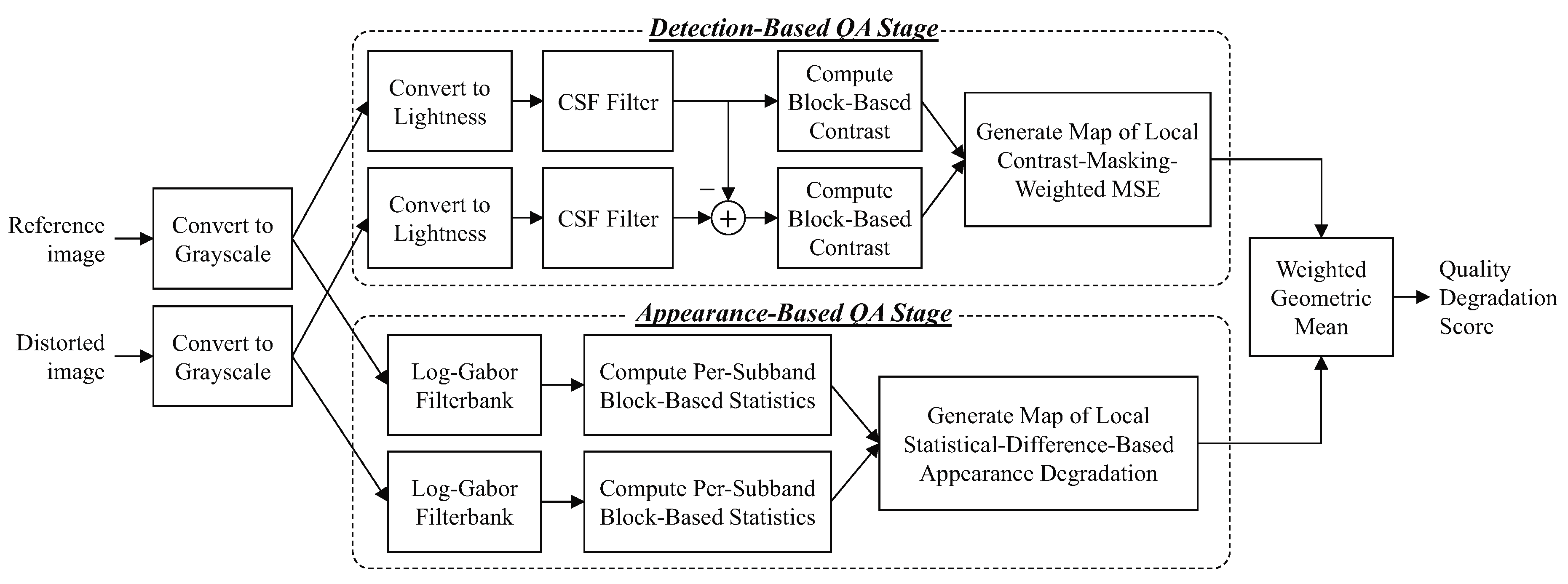
Figure 1 shows a block diagram of MAD’s stages. MAD takes as input two RGB images: a distorted image and its corresponding reference image. Only the luminance information is used, and thus the RGB images are converted to grayscale versions via the pointwise conversion $X=0.299R+0.587G+0.114B$, where R, G, B denote the RGB values and X denotes the resulting grayscale value. In the original Matlab implementation of MAD, this conversion was performed via the rgb2gray function.

The detection stage, represented in the top portion in Figure 1, first converts the images into the lightness domain, then filters the images with a contrast sensitivity function (CSF) filter, and then local block-based statistics are extracted and compared to create a detection-based quality degradation map. In the appearance stage, represented in the lower portion of Figure 1, each image is first decomposed into 20 log-Gabor subbands (5 scales × 4 orientations), then block-based subband statistics are computed and compared for corresponding subbands of the reference and distorted images, and then these block-based statistical differences are merged across bands to create an appearance-based quality degradation map. Finally, the detection-based and appearance-based maps are each collapsed into a scalar quantity, and then the two resulting scalars are then combined into a final quality (degradation) score via a weighted geometric mean.

The following subsections provide details of the implementations of these stages in the original Matlab/C++ versions.

3.1. Visual Detection Stage

As argued in [14], when the amount of distortion is relatively low (i.e., when the distorted image would generally judge to be of high quality), some of the distortions are in the near-threshold regime, and thus the human visual system (HVS) judges quality based on visual detection of the distortions. Thus, the objective of the visual detection stage in MAD is to determine which distortions are visible, and then to perform QA based on these visible distortions. To estimate the visibilities of the distortions, MAD employs a block-based contrast masking measure; this yields a map indicating the local visibility of the distortion in each block. QA is then performed by using local mean squared error (MSE) between the reference and distorted images weighted by the masking map.

In the original Matlab version of MAD, the visual detection stage was implemented as shown in Listing 1.

First, each pixel of reference and distorted images are sent through a pointwise scaling and power function with an exponent of 2.2/3. The scaling and power of 2.2 converts the pixel values into luminance values (assuming an sRGB display). The power of 1/3 provides a basic account of brightness perception (termed “relative lightness” in [14]). The scaling is performed by direct multiplication; the power function is performed via a lookup table.

Next, the HVS’s frequency dependence of contrast sensitivity (CSF function) is modeled by using a lowpass filter. This filter is defined in the frequency domain, and it is applied to both the reference image and the error image via multiplication in the frequency domain. For the original Matlab implementation, the fft2 and ifft2 functions were used to perform the forward and inverse 2D discrete Fourier transforms (DFTs); for the C++ port, the ooura FFT library was used.

Next, a visibility map is created based on a basic measure of contrast masking. The RMS contrast of each $16\times 16$ block of the reference image is compared to the RMS contrast of the distortions (errors) in the corresponding $16\times 16$ block of the distorted image. The corresponding block in the visibility map is assigned an “error visibility” value that is larger for lower contrast reference blocks containing higher contrast distortion (and vice-versa). Note that the standard deviation used in computing the RMS contrast is the modified version defined in [14] as the minimum of the four standard deviations of the $8\times 8$ sub-blocks of each $16\times 16$ block. Also note that overlapping blocks are used; neighboring $16\times 16$ blocks are positioned $\Delta i=4$ and/or $\Delta j=4$ pixels away. For this visibility map, C++ code was used in both the original Matlab implementation (MEX file) and the C++ port.

Listing 1 Pseudocode of MAD’s Visual Detection Stage

1: procedureVisualDetectionQA 2: Inputs and Output: 3:   $im{g}_{ref}\leftarrow \mathrm{grayscale}\mathrm{reference}\mathrm{image}\left(\mathrm{input}M\times N\mathrm{matrix}\right)$ 4:   $im{g}_{dst}\leftarrow \mathrm{grayscale}\mathrm{distorted}\mathrm{image}\left(\mathrm{input}M\times N\mathrm{matrix}\right)$ 5:   $d_{detect}\leftarrow \mathrm{quality}\mathrm{degradation}\mathrm{score}\left(\mathrm{output}\mathrm{scalar}\right)$ 6: Convert Images to Lightness: 7:   $LUT:=k\times {[0:255]}^{2.2/3}$ 8:   $im{g}_{ref}:=LUT\left(im{g}_{ref}\right)$ 9:   $im{g}_{dst}:=LUT\left(im{g}_{dst}\right)$ 10:   $im{g}_{err}:=im{g}_{dst}-im{g}_{ref}$   11: Apply CSF Filter: 12:   $CSF\leftarrow \mathrm{Filter}\mathrm{frequency}\mathrm{response}$ 13:   $im{g}_{ref}:=\mathtt{ifft}\mathtt{2}\left(\mathtt{fft}\mathtt{2}\right($imgref)CSF$)$ 14:   $im{g}_{err}:=\mathtt{ifft}\mathtt{2}\left(\mathtt{fft}\mathtt{2}\right($imgerr)CSF$)$ 15: Build Visibility MapV: 16:   for each 16x16 block $b_{ref}\in im{g}_{ref}$, $b_{err}\in im{g}_{err}\text{@}(i,j)$ do 17:     $\mu \left(b_{ref}\right),\sigma \left(b_{ref}\right)\leftarrow \mathrm{mean}\mathrm{and}\mathrm{standard}\mathrm{deviation}\mathrm{of}{b}_{ref}$ 18:     $\sigma \left(b_{err}\right)\leftarrow \mathrm{standard}\mathrm{deviation}\mathrm{of}{b}_{err}$ 19:     $c\left(b_{ref}\right):=\sigma \left(b_{ref}\right)/\mu \left(b_{ref}\right)$ // RMS contrast of mask 20:     $c\left(b_{err}\right):=\sigma \left(b_{err}\right)/\mu \left(b_{ref}\right)$ // RMS contrast of error 21:     $V_{i,j}\leftarrow \mathrm{visibility}\text{@}(i,j)\mathrm{based}\mathrm{on}c\left(b_{ref}\right)\mathrm{and}c\left(b_{err}\right)$ 22:   end for 23: Compute Quality Degradation Score: 24:   $H\leftarrow 16\mathrm{x}16\mathrm{matrix}\mathrm{with}\mathrm{all}\mathrm{entries}\mathrm{set}\mathrm{to}1/(16\times 16)$ 25:   $D:={im{g}_{err}}^2\ast H$ // LMSE via 2D convolution (imfilter) 26:   $d_{detect}:=\frac{1}{\sqrt{M\times N}}{∥D\times V∥}_F$   27: end procedure

The output of the visual detection stage is a scalar, $d_{detect}$, denoting the overall quality degradation estimate due to visual detection of distortions. As shown in Listing 1, $d_{detect}$ is given as the RMS value of the product of the visibility map and a map of local MSE between the reference and distorted images (following lightness conversion and CSF filtering) measured by using the error image.

3.2. Visual Appearance Stage

When the amount of distortion is relatively high, MAD advocates the use of a different strategy for QA, one based not on visual detection, but on visual appearance. In this visual appearance stage, MAD employs a log-Gabor filterbank to model a set of visual neurons at each location and at various scales. QA is then performed based on local statistical differences between the modeled neural responses to reference image and the modeled neural responses to the distorted image.

In the original Matlab version of MAD, the visual detection stage was implemented as shown in Listing 2.

First, the images are subjected to a log-Gabor filterbank of five scales (center radial spatial frequencies) and four orientations (0, 45, 90, and 135 degrees). This filterbank is designed to mimic an array of linear visual neurons, and thus the centers and bandwidths of the passbands have been selected to approximate the cortical responses of the mammalian visual system. The log-Gabor frequency responses are constructed in the 2D DFT domain, and the filtering is applied via frequency-domain filtering. As shown in Listing 1, the filtering results in 20 subbands for the reference image $\left\{R_{ref,s,o}\right\}$ and 20 subbands for the distorted image $\left\{R_{dst,s,o}\right\}$, each set indexed by scale index s and orientation index o. Again, in Matlab, the fft2 and ifft2 functions were used to perform the forward and inverse 2D DFTs; the ooura FFT library was used for the C++ port.

Listing 2 Pseudocode of MAD’s Visual Appearance Stage

1: procedureVisualAppearanceQA 2:   Inputs and Output: 3:   $im{g}_{ref}\leftarrow \mathrm{grayscale}\mathrm{reference}\mathrm{image}\left(\mathrm{input}M\times N\mathrm{matrix}\right)$ 4:   $im{g}_{dst}\leftarrow \mathrm{grayscale}\mathrm{distorted}\mathrm{image}\left(\mathrm{input}M\times N\mathrm{matrix}\right)$ 5:   $d_{appear}\leftarrow \mathrm{quality}\mathrm{degradation}\mathrm{score}\left(\mathrm{output}\mathrm{scalar}\right)$ 6: Create and Apply Log-Gabor Filters: 7:   for scale $s:=1:5$ do 8:     // (0, 45, 90, 270 degrees) 9:     for orientation $o:=1:4$ do 10:       $G_{s,o}\leftarrow 2\mathrm{D}\mathrm{complex}\mathrm{freq}.\mathrm{resp}.\mathrm{of}\mathrm{filter}\text{@}(s,o)$ 11:       // simulated neural response matrices 12:       $R_{ref,s,o}:=\mathtt{ifft}\mathtt{2}\left(\mathtt{fft}\mathtt{2}\right($imgref)Gs,o$)$ 13:       $R_{dst,s,o}:=\mathtt{ifft}\mathtt{2}\left(\mathtt{fft}\mathtt{2}\right($imgdst)Gs,o$)$ 14:     end for 15:   end for   16: Compute Response Differences (Appearance Changes): 17:   for scale $s:=1:5$ do 18:     $w_s\leftarrow \mathrm{scale}-\mathrm{dependent}\mathrm{weighting}\mathrm{factor}$ 19:      // (0, 45, 90, 270 degrees) 20:     for orientation $o:=1:4$ do 21:       for each block $b_{ref}\in R_{ref,s,o}$, $b_{dst}\in R_{dst,s,o}\text{@}(i,j)$ do 22:          $\sigma \left(b_{ref}\right),\sigma \left(b_{dst}\right)\leftarrow \mathrm{std}.\mathrm{devs}.\mathrm{of}|b_{ref}|\mathrm{and}|b_{dst}|$ 23:          $\varsigma \left(b_{ref}\right),\varsigma \left(b_{dst}\right)\leftarrow \mathrm{skewnesses}\mathrm{of}|b_{ref}|\mathrm{and}|b_{dst}|$ 24:          $\kappa \left(b_{ref}\right),\kappa \left(b_{dst}\right)\leftarrow \mathrm{kurtoses}\mathrm{of}|b_{ref}|\mathrm{and}|b_{dst}|$ 25:          $\eta \leftarrow \mathrm{scalar}\mathrm{of}\mathrm{diffs}.\mathrm{in}\mathrm{above}\mathrm{stats}(\mathrm{ref}\mathrm{vs}.\mathrm{dst})$ 26:          // appearance change @ (i, j) 27:          $A_{i,j}:=A_{i,j}+w_s\times \eta$ 28:         end for 29:       end for 30:     end for   31: Compute Quality Degradation Score: 32:     $d_{appear}:=\frac{1}{\sqrt{M\times N}}{∥A∥}_F$   33: end procedure

Next, each pair of subbands (reference and distorted) is divided into $16\times 16$ blocks, and basic sample statistics (standard deviation, skewness, kurtosis) are computed for each block. These statistics measured for the reference image’s block are compared to the corresponding statistics measured from the co-located block of the distorted image to quantify the appearance change for that location, scale, and orientation ($\eta$). MAD uses a simple sum of absolute differences between the reference and distorted statistics for the computation of $\eta$. These $\eta$ values are then summed across scale and orientation to generate a single map denoting local degradations in appearance. Again, overlapping blocks are used, with $\Delta i=4$ and/or $\Delta j=4$ pixels away.

The output of the visual appearance stage is a scalar, $d_{appear}$, denoting the overall quality degradation estimate due to degradations in visual appearance. As shown in Listing 1, $d_{detect}$ is given as the root mean square (RMS) value of the product of the visibility map and a map of local MSE between the reference and distorted images (following lightness conversion and CSF filtering).

3.3. Overall MAD Score

The overall MAD score is determined based on the following adaptive combination of the $d_{detect}$ and $d_{appear}$,

$$\mathrm{MAD}\mathrm{score}={\left(d_{detect}\right)}^{\alpha }{\left(d_{appear}\right)}^{1-\alpha }$$

(1)

where the adaptive weight $\alpha$ is chosen to give more weight to $d_{detect}$ if the image is in the high-quality regime, and more weight to $d_{appear}$ if the image is in the low-quality regime. The value of $\alpha$ is computed by using a sigmoidal function of $d_{detect}$ (see [14]).

4. CUDA Implementation of MAD

In this section, we describe our GPU-based implementation of MAD, which uses separate CUDA kernels for all fully data-parallel operations.

4.1. CPU Tasks: Loading Images; Computing Overall Quality

The reference and distorted images are first read into the computer’s RAM (the host memory), then converted to grayscale on the CPU, and then converted into linearized single-precision arrays on the CPU. These steps are performed by using the OpenCV library.

The single-precision arrays are then copied to the GPU’s RAM by transferring the data across the PCIexpress (PCIe) bus. For the single-GPU evaluations, in order to minimize latency introduced by PCIe memory traffic, we performed this transfer from the host memory to the GPU memory only once during the beginning of the program. As described previously, and as demonstrated in similar studies [20,22], transferring data to and from the GPU memory creates a performance bottleneck which can result in a latency that can obviate the performance gains. For the multi-GPU evaluation, the arrays were also transferred to each GPU only once at the beginning; however, a considerable number of inter-GPU transfers were required, as discussed later in Section 5.3.

MAD’s detection and appearance stages are computed on the GPU as discussed next. However, because MAD can optionally provide to the end-user the detection-based and appearance-based maps (in addition to the scalar quality scores), we transferred the maps from the GPU back to the CPU, where the maps were collapsed and the individual and overall quality scores were computed. These map transfers can be eliminated in practice if only the scalar scores are sufficient for a particular QA application.

4.2. Visual Detection Stage in CUDA

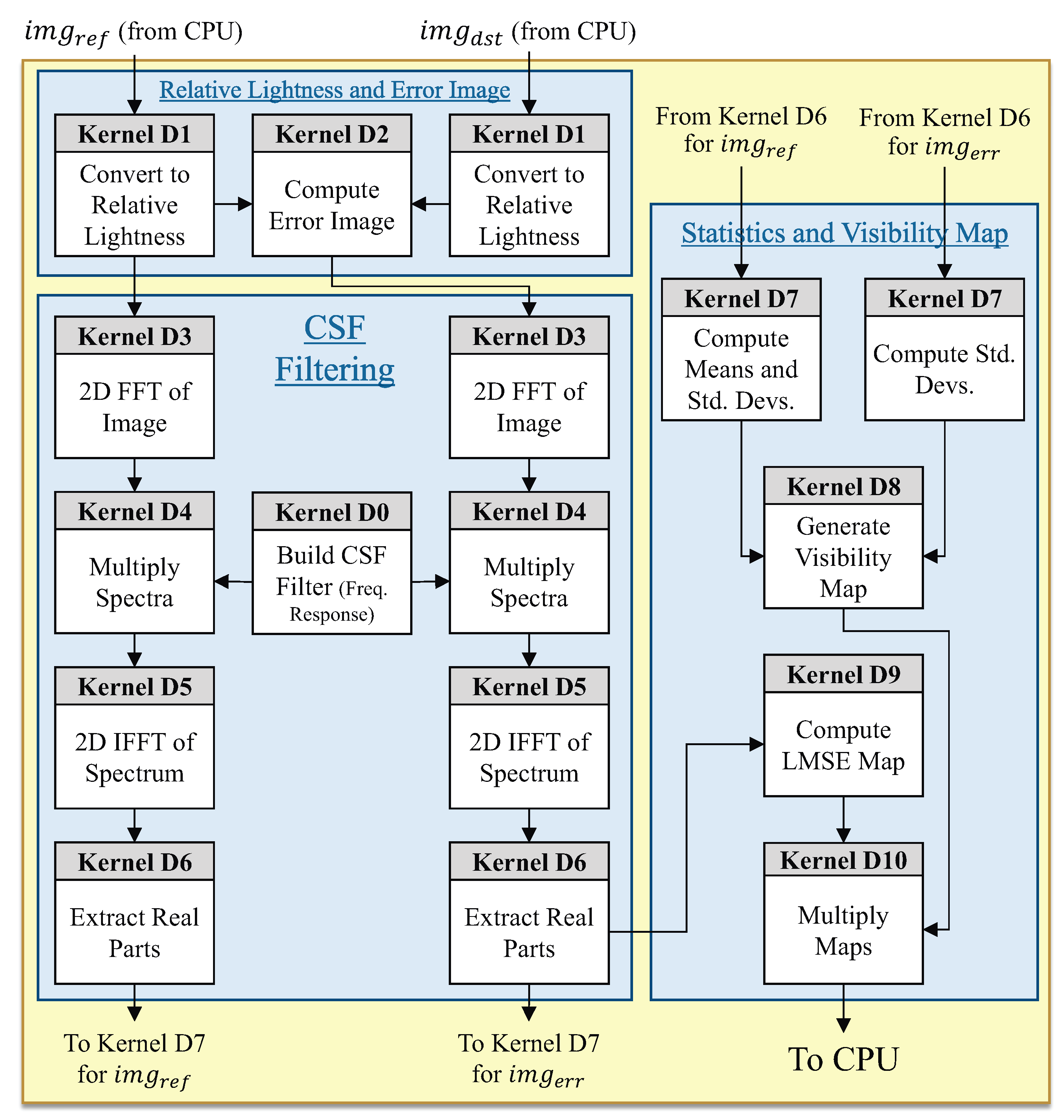
All fully data-parallel operations in our CUDA implementation are performed by individual kernel functions, which are executed such that each CUDA thread performs the kernel-defined operation on a separate pixel of the input image. Figure 2 shows the specific breakdown of how the detection stage was implemented on the GPU via eleven CUDA kernels (Kernels D0-D10).

The relative lightness conversion and CSF filtering are performed by Kernels D0-D6:

• Kernel D0 constructs the CSF filter’s frequency response (Line 12 of Listing 1).
• Kernel D1 maps the images into the relative lightness domain (Lines 7–9).
• Kernel D2 computes the error image (Line 10).
• Kernel D3 computes the 2D DFT (via the cuFFT library) to obtain each image’s spectrum (Lines 13,14).
• Kernel D4 performs multiplication of each image’s spectrum with the CSF frequency response (Lines 13,14).
• Kernel D5 computes the 2D inverse DFT (via the cuFFT library) to transform the images back into the spatial domain (Lines 13–14).
• Kernel D6 extracts the real part of the inverse FFT to avoid roundoff-induced imaginary values (Lines 13,14).

The statistics, visibility map, LMSE map, and final detection-based map are computed by Kernels D7–D10:

• Kernel D7 computes the means and standard deviations of the blocks (Lines 17,18).
• Kernel D8 computes and compares the blocks’ contrasts to generate the distortion visibility map (Lines 19–21).
• Kernel D9 computes the local MSE map from the error image (Lines 24,25).
• Kernel D10 computes the product of the visibility map and the local MSE map (Line 26).

The final detection-based map (visibility-weighted local MSE map from Kernel D10) is transferred back across the PCIe bus to the CPU, where the final detection-based quality degradation estimate $d_{detect}$ is computed.

4.3. Visual Appearance Stage in CUDA

The visual appearance stages was also implemented by using separate kernels for all fully data-parallel operations; the kernel functions are executed such that each CUDA thread performs the kernel-defined operation on a separate pixel of the input image. Figure 3 shows the specific breakdown of how the appearance stage was implemented on the GPU via six CUDA kernels (Kernels A0-A6).

• Kernel A0 computes the 2D DFT of the image via the cuFFT library (fft in Lines 12,13 of Listing 2).
• Kernel A1 builds the frequency response of its log-Gabor filter (Line 10).
• Kernel A2 pointwise multiplies its filter’s frequency response with the image’s spectrum that has been cached in GPU memory (Lines 12,13).
• Kernel A3 performs the inverse 2D DFT via the cuFFT library (ifft in Lines 12,13).
• Kernel A4 takes the magnitude of each complex-valued entry in the response (Lines 22–24).
• Kernel A5 computes three matrices for each subband; each matrix contains the standard deviations, skewnesses, and kurtoses of the 16x16 subband blocks (Lines 22–24).
• Kernel A6 computes the appearance-based quality degradation map (Line 32).

The frequency response of each of the 20 distinct filters are constructed in the DFT domain in a separate instance of Kernel A1. Because each element of the $M\times N$ frequency response is independent of all other elements, we implemented the construction of all frequency response values in separate threads where each overall filter is created by the execution of a 4D CUDA kernel with $M\times N$ total threads; i.e., the kernel is executed as a 2D grid where each thread block within the grid is composed of a 2D collection of threads. The size of the grid was $(M/16)\times (N/16)$ and the size of the thread blocks were $16\times 16$ independent of the size of the input image.

The images are then filtered with each of the log-Gabor filters in Kernel A3, which performs pointwise complex multiplication between each filter instance and the images spectra, which has been stored in global device (GPU) memory after the FFT operation is applied to it in Kernel A0.

After each image has been processed through the filterbank, Kernel A4 performs an inverse FFT for each corresponding log-Gabor subband. The result of the image passing through the filterbank is a set of 20 complex values $M\times N$ subbands. The imaginary component is a result of the odd filter and the real component is a result of the even filter.

Next, in Kernel A5, a set of three statistical matrices (one matrix each for standard deviation, skewness, and kurtosis) from each of the 20 filtered images is computed. Due to the overlapping blocks (shift of the sliding window by four pixels between successive blocks), the size of each statistical matrices is $⌈M/4⌉\times ⌈N/4⌉$.

The set of 60 $⌈M/4⌉\times ⌈N/4⌉$ statistical matrices from the processed reference image are compared against the 60 $⌈M/4⌉\times ⌈N/4⌉$ statistical matrices from the filterbank processing of the distorted image in Kernel A6 to produce the appearance-based quality degradation map. This map is transferred back across the PCIe bus to the CPU, where the final appearance-based quality degradation estimate $d_{appear}$ is computed.

5. Results and Analysis

We evaluated the GPU-based implementation on three systems containing a variety of Nvidia GPUs. Here, we report and discuss the runtime performances.

All performance timings for the GPU-based implementations were performed by using Nvidia’s Nsight profiler. For the test images, we used the CSIQ database [14]. As documented in [22], the semantic category of the reference image did not have a significant effect on MAD’s runtime; however, a minor effect was observed for different distortion types and amounts. Thus, we used two reference images, all six distortion types, and two levels of distortion (high and low) for each type. In a follow-up verification experiment (for Evaluation 1 only), we used all images from the IVC database [60].

5.1. Evaluation 1: Overall and Per-Kernel Performance

The primary test system consisted of a modern desktop computer with an Intel Core i7 processor (Intel Corporation, Santa Clara, CA, USA) and three Nvidia GPUs (two GeForce Titans and one Tesla K40; all use the Kepler GK110 GPU architecture). The details of the primary test system are shown in

Table 1. Details of the primary test system.

CPU	Intel Core i7-4790K CPU @ 4 GHz (Haswell)
	Cores: 4 cores (8 threads)
	Cache: L1: 256 KB; L2: 1 MB; L3: 8 MB
RAM	16 GB GDDR3 @ 1333 MHz (dual channel)
OS	Windows 7 64-bit
Compiler	Visual Studio 2013 64-bit; CUDA 7.5
GPU 1	Nvidia Tesla K40c (PCIe 2.0)
GPU 2	Nvidia GeForce Titan Black (PCIe 3.0)
GPU 3	Nvidia GeForce Titan Black (PCIe 3.0)

. For the primary single-GPU experiment, we used one of the Titans (labeled GPU 2 in Table 1). For the follow-up secondary single-GPU experiment (IVC database), we used a separate system containing a Tesla K40 GPU (labeled as System 2 presented later in Section 5.2).

The results of the performance analysis of the primary single-GPU implementation are shown in

Table 2. Results on the main experiment on the primary test system (CSIQ database; Titan Black).

Code	C++		CUDA
MAD Stage	Time (ms)	% Time	Time (ms)	% Time
Entire Program	958.7	100%	40.2	100%
CSF Filter	77.4	8.1%	0.6	1.4%
Detection Stats.	87.5	9.1%	5.8	14.4%
Log-Gabor Filtering	499.6	52.1%	8.5	21.0%
Appearance Stats.	280.1	29.2%	23.4	58.1%

. The results of the follow-up verification performance analysis of the secondary single-GPU implementation (IVC database) are shown in

Table 3. Results of the follow-up experiment on the secondary test system (IVC database; Tesla K40).

Code	C++		CUDA
MAD Stage	Time (ms)	% Time	Time (ms)	% Time
Entire Program	842.9	100%	55.4	100%
CSF Filter	88.4	10.5%	0.8	1.4%
Detection Stats.	89.8	10.7%	8.2	14.8%
Log-Gabor Filtering	512.8	60.8%	10.1	18.1%
Appearance Stats.	144.0	17.1%	34.3	61.9%

. All single-GPU kernels were executed in a task-serial fashion. Because the subsections of the algorithm did not have any overlap in computation, we were able to easily compute the ratio of the overall time spent on the different subsections vs. the overall runtime of the complete algorithm. Overall, going from a CPU-based implementation to a GPU-based implementation results in a significant speedup. The C++ version required approximately 960 ms, whereas the CUDA version required approximately 40 ms, which is a 24× speedup. The follow-up experiment confirmed these same general per-stage and overall trends (843 ms down to 55 ms), though with a lesser 15× overall speedup due to the lower-spec K40 GPU used in the latter experiment.

A runtime of 40 ms would allow MAD to operate at 25 frames/sec in a video application, which can be considered near-real-time performance, with the caveat that our experiments consider only $512\times 512$ images. Our implementation is expected to scale linearly to larger image sizes, but a formal analysis of this is a topic of future investigation.

Please note that the GPU version of the code is not a simplification nor an approximation of the MAD algorithm. Both the CPU and GPU results yield the same numerical results for practical purposes (differences of less than $1\%$ between the CPU and GPU versions of the MAD quality scores).

5.1.1. Per-Kernel Performance on the Detection Stage

Table 4. Runtimes of the individual kernels.

Kernel	Number of Launches	Average Individual Time ($\mathsf{\mu }$s)	Total Time ($\mathsf{\mu }$s)
D0 - Build CSF Filter	1	134	134
D1 - Map to Luminance	2	20	40
D2 - Difference Image	1	15	15
D3 - Forward FFT	2	69	138
D4 - Filtering	2	25	51
D5 - Inverse FFT	2	55	111
D6 - Keep Real Part Only	2	16	31
D7 - Local Statistics	1	1358	1358
D9 - LMSE	1	4387	4387
D10 - Generate Map	1	45	45
A0 - Forward FFT	2	69	138
A1 - Build log-Gabor Filter	40	170	3393
A2 - Perform Filtering	40	25	1007
A3 - Inverse FFT	40	55	2218
A4 - Take Magnitude	40	30	1184
A5 - Local Statistics	40	560	22,390
A6 - Generate Map	20	44	881

displays the runtimes of all constituent kernels on the primary test system. The first 11 rows of Table 4 show the runtimes of the individual kernels for MAD’s detection stage. In the detection stage, Kernel D1, which maps the image to the relative lightness domain, performs a scaling of each pixel value by a constant k and then exponentiates the result by the power 2.2/3. This operation achieves the exponentiation through the use the pow function from the CUDA Math library. Kernel D1 is one of the fastest-performing kernels in our program. This kernel, along with Kernels D3, D4, D6, and D10, all are composed of standard arithmetic operations with no control flow (e.g., no if/else statements). The lack of control flow ensures there is minimal thread divergence in these kernels. Thread divergence occurs when threads within the same warp (group of 32 threads) take different paths of execution, which causes all threads in the warp to wait on the completion of the slowest-performing thread.

The forward and inverse FFTs, which are used in Kernels D3 and D5, exhibit relatively good performance in regards to runtime. Their fast execution is expected because the CUDA FFT library we utilized, called cuFFT, is based on the popular FFTW library [61]; and, as in FFTW, calls to CUDA’s FFT function autonomously fine-tune their implementation details based on the hardware on which they are executed.

Kernels D7 and D8 are the worst-performing kernels in the detection stage. We attribute the poor performance of Kernel D7, which is the kernel that performs the detection-based statistical computations, to the redundant computations in our specific implementation. The integral image technique is currently being explored to reduce the number of operations performed in this kernel. Kernel D8, which computes the local MSE between the reference and distorted image, performs a large number of control flow logic. It is likely that the large amount of control flow gives rise to undesired thread divergence. We are currently investigating potential reformulations of the specific algorithm used in this kernel to exploit more parallelism to avoid the suspected thread divergence.

5.1.2. Per-Kernel Performance on the Appearance Stage

The lower seven rows of Table 4 show the runtimes of the individual kernels for MAD’s appearance stage. The appearance stage consumes the majority of the overall runtime. The primary reason for the relatively massive runtime of this section is simply that the filterbank is itself massive in regards to the number of computations of the overall algorithm. Each filter in the pair of filterbanks (one filterbank each for the reference and distorted images) is composed of 20 different filtering sections, which are represented as the individual columns as shown in Figure 4.

Kernels A2 and A4 are expected to have good runtime performance due to their lack of control flow. Indeed, the data in Table 4 support this expectation; Kernels A2 and A4 are the fastest-performing kernels in this stage of the algorithm.

Because the coefficients of the 20 different log-Gabor filters are only dependent on the dimensions of the input image, and not on the image’s actual pixel data, we initially attempted to precompute these filter coefficients. However, we found that it was far more advantageous to simply compute the coefficients at the time of their use in the filterbank, as opposed to retrieving the coefficient values from global memory. We suspect that the pre-computational process gave rise to poor spatial locality (i.e., the filter coefficients were stored further away from the actual computations performed), thus eliminating the expected performance gain.

The key conclusions from this experiment are as follows. Exploiting the parallel hardware paths in a GPU through a CUDA-based implementation of MAD leads to a 24× speedup, and a runtime of 40 ms. A deeper look on a per-kernel basis reveals that computation of the local MSE map (Kernel D9) takes the most time in the detection stage and the computation of block-based statistics (Kernel A5) takes the most time in the appearance stage. We believe the use of shared memory to perform local computation within the blocks in on-chip SRAM would alleviate this bottleneck. Just as performing computation in a block-based fashion to exploit the memory hierarchy is critical to good performance on modern CPUs [62] utilization of the memory hierarchy on GPUs is also a critical, but relatively advanced, optimization technique. Thus, a detailed understanding of the memory system in the GPU is essential to further improve performance.

5.2. Evaluation 2: Performances on Different GPUs

Next, we investigated the effects that GPUs with different architectures/capabilities might have on the runtimes. For this evaluation, we ran the code on two additional systems, the details of which are provided in

Table 5. Details of the systems containing different GPUs (the specific GPU employed on each system is shown in boldface).

Part	System 1 (Repeated from Table 1)	System 2	System 3
2]*CPU	Intel Core i7-4790K CPU @ 4 GHz	Intel Xeon E5-1620 @ 3.70 GHz	Intel Core i7-4790K CPU @ 4 GHz
	Cores: 4 cores (8 logical)	Cores: 4 cores (8 logical)	Cores: 4 cores (8 logical)
	Cache: L1/2/3: 256 KB/1 MB/8 MB	Cache: L1/2/3: 256 KB/1 MB/10 MB	Cache: L1/2/3: 256 KB/1 MB/8 MB
RAM	16 GB DDR3 @ 1333 MHz (dual channel)	24 GB DDR3 @ 1866 MHz (dual channel)	16 GB DDR3 @ 1866 MHz (dual channel)
OS	Windows 7 64-bit	Windows 7 64-bit	Windows 10 Pro 64-bit
Compiler	Visual Studio 2013 64-bit; CUDA 7.5	Visual Studio 2013 64-bit; CUDA 7.5	Visual Studio 2013 64-bit; CUDA 7.5
GPU 1	Nvidia Tesla K40c (PCIe 2.0)	Nvidia Tesla K40 (PCIe 3.0)	Nvidia GeForce GTX 960 (PCIe 3.0)
GPU 2	Nvidia GeForce Titan Black (PCIe 3.0)	Nvidia NVS 310 (PCIe 3.0)	-
GPU 3	Nvidia GeForce Titan Black (PCIe 3.0)	-	-

. The setup listed in Table 5 as System 1 was the same system used in the previous section (Evaluation 1); we have repeated its specifications here for convenience. System 2 used an Nvidia Tesla K40, which is a high-end GPU designed primarily for scientific computation. System 3 used an Nvidia GTX 960 GPU, which is designed primarily for gaming.

The results of this evaluation are shown in

Table 6. Results on systems with different GPUs.

Code	System 1 (Titan Black)		System 2 (Tesla K40)		System 3 (GTX 960)
MAD Stage	Time (ms)	% Time	Time (ms)	% Time	Time (ms)	% Time
Entire Program	40.2	100%	64.5	100%	74.2	100%
CSF Filter	0.6	1.4%	0.8	1.2%	1.4	1.9%
Detection Stats.	5.8	14.4%	8.2	12.7%	7.1	9.6%
Log-Gabor Filtering	8.5	21.0%	16.0	24.7%	32.7	44.1%
Appearance Stats.	23.4	58.1%	38.5	59.7%	31.2	42.1%
PCIe Transfers	0.8	1.9%	0.4	1.1%	0.6	1.0%

, which shows the overall runtime as well as the runtimes of the specific stages of MAD. Before discussing the observed execution times, it is important to note the differences in the hardware configuration and capabilities of the three GPUs; these specifications are shown in

Table 7. Hardware configuration and capabilities of the three GPUs.

Property	Titan Black	Tesla K40	GTX 960
Architecture	Kepler GK110B	Kepler GK110B	Maxwell GM206
Single-Precision CUDA Cores	$192\times 14$	$192\times 15$	$128\times 8$
GPU Frequency	875 MHz	745 MHz	1178 MHz
Single-Precision Computational Throughput	5.12 Tflops	4.39 Tflops	2.31 Tflops

.

GPUs are considered to be highly threaded, many-core processors that provide a very large computational throughput. This large throughput can be used to hide unavoidable memory latencies by utilizing the GPU’s ability to execute a very large number of threads. The large memory bandwidth can also be used to hide memory latency. The achieved performance, therefore, depends on the parallelism exploited by the algorithm, the effectiveness of latency hiding, and the utilization of multiprocessors (occupancy) [63]. Based on the results in Table 6, observe that our CUDA implementation exhibits better performance and a shorter runtime on the Titan than on the GTX 960. This observation indicates that the implementation is effective in scaling related to cores: The Titan has 2688 cores and the GTX 960 has 1024 cores.

In our current CUDA implementation, most kernels launch as more than 200,000 concurrent threads for the specific dataset used for our experiment. One of the limiting factors of the number of threads that can be executed simultaneously is the overall number of cores on the GPU. The maximum number of threads that can be executing at any given time is the same as the number of cores on the GPU. Therefore, the larger runtime on the GTX 960 can be attributed to its fewer number of cores. The speedup can as well be attributed to the minimal use of inter-thread communication in our implementation. Code that depends on the communication of data between threads requires explicit synchronization, which often increases overall runtime. As can be seen in Table 6, the latency of memory transfers across the PCIe memory bus on the Titan is 1.8× of that on the Tesla, and 1.2× of that on the GTX 960. Approximately 2% of the overall runtime is spent on PCIe memory transfer on the Titan.

On the GeForce line of Nvidia GPUs (Titan Black and GTX 960), cudaMalloc (the function call used to allocate GPU memory in the CUDA programming model) not only allocates the memory on the GPU, but also initializes the contents to zero, which emulates the C-language calloc function. However, on the Tesla line of Nvidia GPUs (Tesla K40), cudaMalloc simply allocates the memory on the GPU, leaving garbage data in the allotted memory, emulating the C-language malloc function. This necessitates additional cudaMemcpy calls to initialize the memory allocated on the Tesla K40 to avoid garbage values.

The key conclusions from this experiment are as follows. First, we observe the CUDA implementation of MAD is robust and works well on three GPUs with different internal architectures and capabilities. Second, the CUDA implementation exploits parallelism effectively on all these GPUs without any modification to the code, because the performance scales with the number of cores, as opposed to the frequency at which the cores operate.

5.3. Evaluation 3: Performance on a Multi-GPU System

In this section we analyze the runtime performance when simultaneously utilizing all of the GPUs on System 1. In general, the most straightforward method of utilizing multiple GPUs is to divide the task-independent portions of an algorithm among the different GPUs. MAD’s detection and appearance stages do not share any information until the final computation of the quality score; thus, these two stages are easily performed on separate GPUs. The appearance stage can be further decomposed into a largely task-parallel structure by observing that the subbands produced from filtering the reference and distorted images with the log-Gabor filters are not needed together until computing the difference map. Together, the filterbank and the statistics extracted from each subband consume the majority of the overall runtime. Therefore, implementing each of the two filterbanks, and subsequent statistics extractions, on separate GPUs in parallel has the potential to significantly reduce overall runtime.

Thus, we performed the detection stage on one GPU (System 1’s GPU 1: Tesla K40c), and the two filterbanks were placed on the remaining two GPUs (System 1’s GPU 2 and GPU 3: Titan Black). We chose to perform the detection stage on GPU 1 because this stage requires only three memory transfers: two 1 MB transfers from the host to copy the image data onto the GPU, and one transfer to copy the detection-based statistical difference map back to the host upon completion of the detection stage. Because GPU 1 used a PCIe 2.0 bus, the three memory transfers were able to occur in parallel to the computation on the other two GPUs.

We placed each of the two filterbanks and each subsection’s statistical extraction on neighboring GPUs. The 20 individual sections of the filterbank and their subsequent statistical extraction for each image were performed in parallel on GPU 2 and GPU 3, respectively. We then collected all of the statistical matrices onto GPU 2, and performed the difference map computation. Due to the need to collect all the statistical data from both filterbanks together to compute the difference map, we had to perform a memory transfer between GPU 2 and GPU 3 by using the host as an intermediary. Upon completion of the detection stage and appearance stage, we copied their maps back to the host memory to collapse the maps and calculate the final quality score on the CPU.

The requirement of using the host memory as a buffer forced us to perform a large number of memory transfers across the PCIe bus. In the single-GPU implementation, we only used two 1 MB data transfers at the beginning of the program to get the image data to the GPU, and two 1 MB transfers back to the CPU to collapse and combine the statistical difference maps. Decomposing the filterbank into task-parallel sections, as previously described, causes the number of data transfers across the PCIe bus to increase to 126 memory transfers.

The results of the performance analysis of the multi-GPU implementation are shown in

Table 8. Results of the multi-GPU implementation.

Task	Single GPU	Three GPUs
Entire Program	40.2 ms	28.9 ms
Total PCIe Memory Transfers	4	126
Latency from PCIe Transfers	0.4 ms	0.9 ms
GPU Overlap	n/a	19.5 ms
GPU Activity	38.9 ms	20.6 ms

. A 1.4× speedup is observed in the overall execution time. While an ideal speedup going from one GPU to three GPUs would be 3×, the somewhat lower 1.4× speedup is not surprising. As explained in the preceding paragraphs, a large number of memory transfers (126) were necessary to facilitate task-parallelism, and these would have resulted in a significant slowdown had we not been able to overlap the memory transfers with computation.

This brief study on parallelizing MAD across three GPUs provides two important lessons for attempting to implement a highly parallel version of MAD or other similar programs on multi-GPU-based high-performance nodes. One, division of tasks between the GPUs should be as clean as possible, as communication, data transfer and synchronization will reduce the gains obtained from parallelization. Two, in the event that certain data-bound dependencies exist and require data transfers across GPUs, sub-partitioning such that a data transfer can be parallelized with computation, is highly recommended.

5.4. Evaluation 4: Microarchitectural Analysis of Kernel A5

Finally, we performed a deeper investigation of Kernel A5, the current bottleneck, from the point of view of resource usage. Because Kernel A5 consumes a large portion of the overall runtime, it is pertinent to investigate its interaction with the underlying hardware. This experiment was performed on System 2 described in Table 5.

As described in Section 3, Kernel A5 computes the local statistics (mean, skewness, kurtosis, and standard deviation) of each block via a sliding window using a block size 16 × 16. The specific details of how this kernel was implemented are as follows:

• Every thread declares a 1D array of 256 elements.
• Each thread gathers the 16 × 16 data from the global memory and stores the data in the threads designated local memory space.
• Each thread then computes the sample mean from these 256 elements via a 1D traversal.
• Using the mean an additional 1D traversal is used to calculate the standard deviation, skewness, and kurtosis.
• The calculated values are scattered across the corresponding memory locations in global memory.

In the K40 hardware, there are 64 active warps per streaming multiprocessor (SM). Specifically, the active warps/SM = (number of warps/block) × (number of active blocks/SM) = 8 × 8 = 64 active warps/SM. Hence, a kernel capable of spanning 64 active warps at any point in execution will give a theoretical occupancy of 100%. However, the runtime statistics for Kernel A5 given by the Nsight profiler revealed an average occupancy of only 51.4% occupancy, indicating that only half the number of active warps, 32 as opposed to 64, were used. This finding can be attributed to the kernel launch parameters.

Specifically, Kernel A5 is launched with a grid configuration of $(8,8,1)$ and a block configuration of $(16,16,1)$. Hence, the total number of threads = 8 × 8 × 16 × 16 = 16,384. The number of warps = total number of threads/number of threads in a warp = 16384/32 = 512. The total number of active warps supported = 64 × number of SM on the GPU = 64 × 15 = 960. Thus, in this configuration, the theoretical value of achieved occupancy = 512/960 = 53.33%, and our implementation achieved close to that value.

To further evaluate the development process guided by the profiler, we thus profiled Kernel A5 in terms of memory bandwidth. The memory bandwidth is the rate at which data is read or written from the memory. On a GPU, the bandwidth depends on efficient usage of the memory subsystem, which involves L1/shared memory, L2 cache, device memory, and system memory (via PCIe). Since there are many components in the memory subsystem, we performed separate profiling to collect data from the corresponding subsystem. Memory statistics were collected from:

• Global: Profiling of memory operations to the global memory, with a specific focus on the communication between SMs and L2 cache.
• Local: Profiling of memory operations to the local memory, with a specific focus on the communication between the SMs and the L1 cache.
• Cache: Profiling of communication between L1 cache/texture cache and L2 cache for all memory operations.
• Buffers: Profiling of communication between L2 cache and device memory and system memory.

Figure 5 shows the results of this analysis, which are discussed in the following subsections. Note that the memory statistics of atomics, texture, and shared memory were not collected because our current implementation does not use those features.

5.4.1. Memory Statistics—Global

Global device memory can be accessed through two different data paths. Data traffic can go through L2 and/or L1, and read-only global memory access can alternatively go through the read-only data cache/texture cache. Figure 5 shows that cached loads use the L1 cache or texture cache as well as L2 cache, whereas uncached loads uses only the L2 cache.

On the Tesla K40, the L1 cache line size is 128 bytes. Memory accesses that are cached in both L1 and L2 are serviced with a 128-byte cache line size. Memory accesses that are cached only in L2 are serviced with 32-byte cache line size. This scheme is designed to reduce over-fetch, for instance, in case of scatter memory operations.

A warp in execution accessing device memory (load or store assembly instructions), coalesces the memory accesses of all the threads (32 threads share a program counter) in a warp into one or more of these memory transactions depending on the size of the word accessed by each thread as well as the distribution of the memory addresses across the threads. If all the threads within a warp perform random strides, coalescing gets disturbed, resulting in 32 different accesses in a warp.

Figure 5 shows the average number of L1 and L2 transactions required per executed global memory instruction, separately for load and store operations; lower numbers are better. Ideally, there should be just one transaction for a 4-byte access (32 threads × 4 bytes = 128-byte cache line), and two transactions for an 8-byte access (32 threads × 8 bytes = 256 bytes; 2 cache lines) access.

A memory “request” is an instruction, which accesses memory, and a “transaction” is the movement of a unit of data between two regions of memory. As shown in Figure 5, 129,024 load requests are made in Kernel A5, resulting in 2,256,000 transactions. Each of the requests are 4-byte requests (float). Hence, the number of transactions for a load = 2,256,000/129,024 = 17.485, and the number of transactions for a store = 23,625/1512 = 15.625.

5.4.2. Memory Statistics—Local

Local memory is called local to define its scope from the programmer’s perspective, i.e., it is not global or shared across threads. However, its physical manifestation depends on how much local memory a thread requests. Ideally, if a thread requests only as much memory as can fit in the registers, then the local memory is physically local as well, and accesses are fast. On the other hand, if the requested memory exceeds register capacity, then in a process called spilling, the memory is allocated on the much slower device DRAM. Arrays that are declared in the kernel are automatically saved in global memory. In addition, if there are not enough registers to accommodate all auto variables (register spilling), the variables are saved in local memory.

Every thread can use maximum of 32 registers. If a kernel uses more than 32 registers, then the data gets spilled over to the local memory. Every thread executed in Kernel A5 declares a local storage of 256 elements. The launch configuration of the kernel has 256 threads per block. The total local memory needed by a block = 256 threads × 256 elements per thread × 4-byte each = 262,144 bytes = 256 KB. The on-chip memory of an SM in the Tesla K40 is of size 48 KB. Hence, the register spill gets carried over to global memory, resulting in poor performance because global memory incurs a 200–400 cycle latency.

5.4.3. Memory Statistics—Caches

On Nvidia GPUs, there are three data caches: L1, L2 and texture/read-only. If the data is present in both L1 and L2, 128-byte cache line transactions occur; otherwise 32-byte transactions occur. If the data block is cached in both L2 and L1, and if every thread in a warp accesses a 4-byte value from random sparse locations that miss in L1 cache, each thread will give rise to one 128-byte L1 transaction and four 32-byte L2 transactions. This scenario will cause the load instruction to reissue 32 times more than the case in which the values were adjacent and cache-aligned. Here, the cache hit rate is very low because, by default on the Tesla K40, L1 is not used for load/store purposes.

In summary, the key observation from this microarchitectural analysis of Kernel A5 is that algorithms/programs that target the memory hierarchy of CPUs work poorly with the GPU memory infrastructure. Indeed, GPUs are designed to mostly stream data, while CPU caches are built to capture temporal locality, i.e., reuse data. A second important observation is that it is crucial to understand the concept of warps, and the fact that 32 threads in a warp can access 32 data elements in a single load or store as long as they are contiguous. Thus, when designing CUDA kernels, the programmer must carefully choose the dimensions such that threads in a warp do not access non-contiguous memory. A third observation is that it is important to limit the amount of data that a thread tries to access, because any access that exceeds the 32 registers will result in register spilling, which is an expensive operation.

Overall, this microarchitectural analysis reveals that the default settings for compilation leave the code unoptimized, resulting in millions of unnecessary transfers between device DRAM and the caches. In order to achieve better performance, additional studies on the memory usage are required, and future designs should attempt to reduce the traffic between on-chip and off-chip memories (see [64] for some initial steps).

6. Conclusions

Obtaining performance gains through GPGPU solutions is an attractive area of research. In this paper, we have proposed, analyzed, and discussed a GPU-based implementation of a top-performing perceptual QA algorithm (MAD). Our results demonstrated that going from a CPU-based implementation to a GPU-based implementation resulted in a 15×-24× speedup, resulting in a near-real-time version of MAD that is not an approximation of the original version. Our CUDA implementation was also shown to port well to GPUs with different architectures and capabilities. Our results also demonstrated that obtaining performance gains from utilizing multiple GPUs is a challenging problem with higher potential performance gains; the challenge lies in decomposing the computations into a largely task-parallel algorithmic form. If data must be communicated between the tasks placed on separate GPUs, the memory bandwidth bottleneck can prohibit potential gains. To accommodate for the limited PCIe bandwidth, an appropriate strategy must be formulated and tailored to the problem and particular microarchitectural resources of the GPUs.

One of the broader conclusions from this work is that obtaining performance gains through GPU solutions, especially when utilizing multiple GPUs, requires an understanding of the underlying architecture of the hardware, including the CPU, GPU, and their associated memory hierarchies and bus bandwidths. Although programming APIs, such as CUDA, strive to free the programmer from this burden, they have not yet accomplished this goal.

The second conclusion that can be drawn from this work is that a large number of computational problems can hide the latency introduced by asynchronous memory transfers in the manner proposed in this work. The strategy we found to be best suited for a problem that requires many memory transfers, was to overlap computation with asynchronous memory transfers. Thus, we highly recommend considering this technique for image and video quality assessment algorithms.

References

- Zhang, F.; Ma, L.; Li, S.; Ngan, K.N. Practical Image Quality Metric Applied to Image Coding. IEEE Trans. Multimedia 2011, 13, 615–624. [Google Scholar] [CrossRef]
- Schilling, D.; Cosman, P.C. Image quality evaluation based on recognition times for fast image browsing applications. IEEE Trans. Multimedia 2002, 4, 320–331. [Google Scholar] [CrossRef] [Green Version]
- Hameed, A.; Dai, R.; Balas, B. A Decision-Tree-Based Perceptual Video Quality Prediction Model and Its Application in FEC for Wireless Multimedia Communications. IEEE Trans. Multimedia 2016, 18, 764–774. [Google Scholar] [CrossRef]
- Ma, L.; Xu, L.; Zhang, Y.; Yan, Y.; Ngan, K.N. No-Reference Retargeted Image Quality Assessment Based on Pairwise Rank Learning. IEEE Trans. Multimedia 2016, 18, 2228–2237. [Google Scholar] [CrossRef]
- Rainer, B.; Petscharnig, S.; Timmerer, C.; Hellwagner, H. Statistically Indifferent Quality Variation: An Approach for Reducing Multimedia Distribution Cost for Adaptive Video Streaming Services. IEEE Trans. Multimedia 2017, 19, 849–860. [Google Scholar] [CrossRef]
- Ma, L.; Li, S.; Zhang, F.; Ngan, K.N. Reduced-reference image quality assessment using reorganized DCT-based image representation. IEEE Trans. Multimedia 2011, 13, 824–829. [Google Scholar] [CrossRef]
- Gu, K.; Zhai, G.; Yang, X.; Zhang, W. Using Free Energy Principle For Blind Image Quality Assessment. IEEE Trans. Multimedia 2015, 17, 50–63. [Google Scholar] [CrossRef]
- Shao, F.; Li, K.; Lin, W.; Jiang, G.; Dai, Q. Learning Blind Quality Evaluator for Stereoscopic Images Using Joint Sparse Representation. IEEE Trans. Multimedia 2016, 18, 2104–2114. [Google Scholar] [CrossRef]
- Chandler, D.M. Seven Challenges in Image Quality Assessment: Past, Present, and Future Research. ISRN Signal Process. 2013, 2013, 905685. [Google Scholar] [CrossRef]
- Vu, P.V.; Chandler, D.M. A fast wavelet-based algorithm for global and local image sharpness estimation. IEEE Signal Process. Lett. 2012, 19, 423–426. [Google Scholar] [CrossRef]
- Wang, Z.; Bovik, A.; Sheikh, H.; Simoncelli, E. Image Quality Assessment: From Error Visibility to Structural Similarity. IEEE Trans. Image Process. 2004, 13, 600–612. [Google Scholar] [CrossRef] [PubMed] [Green Version]
- Chandler, D.M.; Hemai, S.S. VSNR: A Wavelet-Based Visual Signal-to-Noise Ratio for Natural Images. IEEE Trans. Image Process. 2007, 16, 2284–2298. [Google Scholar] [CrossRef]
- Lai, Y.; Kuo, C.J. Image quality measurement using the Haar wavelet. In Proceedings of the SPIE: Wavelet Applications in Signal and Image Processing V, San Diego, CA, USA, 27 July–1 August 1997. [Google Scholar]
- Larson, E.C.; Chandler, D.M. Most apparent distortion: Full-reference image quality assessment and the role of strategy. J. Electron. Imaging 2010, 19, 011006. [Google Scholar]
- Vu, C.; Chandler, D.M. S3: A Spectral and Spatial Sharpness Measure. In Proceedings of the 2009 First International Conference on Advances in Multimedia, Colmar, France, 20–25 July 2009. [Google Scholar]
- Wang, R.; Luo, J.; Jiang, X.; Wang, Z.; Wang, W.; Li, G.; Gao, W. Accelerating Image-Domain-Warping Virtual View Synthesis on GPGPU. IEEE Trans. Multimedia 2017, 19, 1392–1400. [Google Scholar] [CrossRef]
- Momcilovic, S.; Ilic, A.; Roma, N.; Sousa, L. Dynamic Load Balancing for Real-Time Video Encoding on Heterogeneous CPU+GPU Systems. IEEE Trans. Multimedia 2014, 16, 108–121. [Google Scholar] [CrossRef]
- Zhang, Z.; Seah, H.S.; Quah, C.K.; Sun, J. GPU-Accelerated Real-Time Tracking of Full-Body Motion With Multi-Layer Search. IEEE Trans. Multimedia 2013, 15, 106–119. [Google Scholar] [CrossRef]
- Ryoo, S.; Rodrigues, C.I.; Baghsorkhi, S.S.; Stone, S.S.; Kirk, D.B.; Hwu, W.W. Optimization Principles and Application Performance Evaluation of a Multithreaded GPU Using CUDA. In Proceedings of the 13th ACM SIGPLAN Symposium on Principles and Practice of Parallel Programming, Salt Lake City, UT, USA, 20–23 February 2008; ACM: New York, NY, USA, 2008; pp. 73–82. [Google Scholar] [CrossRef]
- Gordon, B.; Sohoni, S.; Chandler, D. Data handling inefficiencies between CUDA, 3D rendering, and system memory. In Proceedings of the 2010 IEEE International Symposium on Workload Characterization (IISWC), Atlanta, GA, USA, 2–4 December 2010; pp. 1–10. [Google Scholar]
- Liu, D.; Fan, X.Y. Parallel program design for JPEG compression encoding. In Proceedings of the 2012 9th International Conference on Fuzzy Systems and Knowledge Discovery (FSKD), Chongqing, China, 29–31 May 2012; pp. 2502–2506. [Google Scholar] [CrossRef]
- Phan, T.D.; Shah, S.K.; Chandler, D.M.; Sohoni, S. Microarchitectural analysis of image quality assessment algorithms. J. Electron. Imaging 2014, 23, 013030. [Google Scholar] [CrossRef] [Green Version]
- Pedersen, M. Evaluation of 60 full-reference image quality metrics on the CID:IQ. In Proceedings of the 2015 IEEE International Conference on Image Processing (ICIP), Quebec City, QC, Canada, 27–30 September 2015; pp. 1588–1592. [Google Scholar] [CrossRef]
- Vu, P.V.; Chandler, D.M. ViS3: An algorithm for video quality assessment via analysis of spatial and spatiotemporal slices. J. Electron. Imaging 2014, 23, 013016. [Google Scholar] [CrossRef]
- Andalibi, M.; Chandler, D.M. Digital Image Watermarking via Adaptive Logo Texturization. IEEE Trans. Image Process. 2015, 24, 5060–5073. [Google Scholar] [CrossRef] [PubMed]
- Suda, R.; Aoki, T.; Hirasawa, S.; Nukada, A.; Honda, H.; Matsuoka, S. Aspects of GPU for General Purpose High Performance Computing. In Proceedings of the 2009 Asia and South Pacific Design Automation Conference (ASP-DAC’09), Yokohama, Japan, 19–22 January 2009; IEEE Press: Piscataway, NJ, USA, 2009; pp. 216–223. [Google Scholar]
- Okarma, K.; Mazurek, P. GPGPU Based Estimation of the Combined Video Quality Metric. In Image Processing and Communications Challenges 3; Choras, R., Ed.; Springer: Berlin/Heidelberg, Germany, 2011; Volume 102, pp. 285–292. [Google Scholar]
- Phan, T.; Sohoni, S.; Chandler, D.M.; Larson, E.C. Performance-analysis-based acceleration of image quality assessment. In Proceedings of the 2012 IEEE Southwest Symposium on Image Analysis and Interpretation, Santa Fe, NM, USA, 22–24 April 2012; pp. 81–84. [Google Scholar] [CrossRef]
- Xu, S.; Liu, X.; Jiang, S. A Fast Feature Similarity Index for Image Quality Assessment. Int. J. Signal Process. Image Process. Pattern Recognit. 2015, 8, 179–194. [Google Scholar] [CrossRef]
- Zhang, L.; Zhang, D.; Mou, X. FSIM: A feature similarity index for image quality assessment. IEEE Trans. Image Process. 2011, 20, 2378–2386. [Google Scholar] [CrossRef] [PubMed]
- Chen, M.J.; Bovik, A.C. Fast structural similarity index algorithm. J. Real-Time Image Process. 2011, 6, 281–287. [Google Scholar] [CrossRef]
- Wang, Z.; Simoncelli, E.; Bovik, A. Multiscale structural similarity for image quality assessment. In Proceedings of the Conference Record of the Thirty-Seventh Asilomar Conference on Signals, Systems and Computers, Pacific Grove, CA, USA, 9–12 November 2003; Volume 2, pp. 1398–1402. [Google Scholar]
- Porikli, F. Integral histogram: A fast way to extract histograms in Cartesian spaces. In Proceedings of the 2005 IEEE Computer Society Conference on Computer Vision and Pattern Recognition, San Diego, CA, USA, 20–25 June 2005; Volume 1, pp. 829–836. [Google Scholar]
- Sheikh, H.R.; Bovik, A.C. Image information and visual quality. IEEE Trans. Image Process. 2006, 15, 430–444. [Google Scholar] [CrossRef] [PubMed] [Green Version]
- Gu, K.; Zhai, G.; Yang, X.; Zhang, W. Deep learning network for blind image quality assessment. In Proceedings of the 2014 IEEE International Conference on Image Processing (ICIP), Paris, France, 27–30 October 2014; pp. 511–515. [Google Scholar]
- Kang, L.; Ye, P.; Li, Y.; Doermann, D. Convolutional neural networks for no-reference image quality assessment. In Proceedings of the IEEE Conference on Computer Vision and Pattern Recognition, Columbus, OH, USA, 23–28 June 2014; pp. 1733–1740. [Google Scholar]
- Li, Y.; Po, L.M.; Xu, X.; Feng, L.; Yuan, F.; Cheung, C.H.; Cheung, K.W. No-reference image quality assessment with shearlet transform and deep neural networks. Neurocomputing 2015, 154, 94–109. [Google Scholar] [CrossRef]
- Bosse, S.; Maniry, D.; Wiegand, T.; Samek, W. A deep neural network for image quality assessment. In Proceedings of the 2016 IEEE International Conference on Image Processing (ICIP), Phoenix, AZ, USA, 25–28 September 2016; pp. 3773–3777. [Google Scholar]
- Jia, S.; Zhang, Y.; Agrafiotis, D.; Bull, D. Blind high dynamic range image quality assessment using deep learning. In Proceedings of the 2017 IEEE International Conference on Image Processing (ICIP), Beijing, China, 17–20 September 2017; pp. 765–769. [Google Scholar]
- Kim, J.; Lee, S. Deep learning of human visual sensitivity in image quality assessment framework. In Proceedings of the 2017 IEEE Conference on Computer Vision and Pattern Recognition (CVPR), Honolulu, HI, USA, 21–26 July 2017. [Google Scholar]
- Kim, J.; Nguyen, A.D.; Lee, S. Deep CNN-based blind image quality predictor. IEEE Trans. Neural Netw. Learn. Syst. 2018, PP, 1–14. [Google Scholar] [CrossRef] [PubMed]
- Bianco, S.; Celona, L.; Napoletano, P.; Schettini, R. On the use of deep learning for blind image quality assessment. Signal Image Video Process. 2018, 12, 355–362. [Google Scholar] [CrossRef]
- Moreland, K.; Angel, E. The FFT on a GPU. In Proceedings of the ACM SIGGRAPH/EUROGRAPHICS Conference on Graphics Hardware, San Diego, CA, USA, 26–27 July 2003; Eurographics Association: Aire-la-Ville, Switzerland, 2003; pp. 112–119. [Google Scholar]
- Fialka, O.; Čadik, M. FFT and convolution performance in image filtering on GPU. In Proceedings of the Tenth International Conference on Information Visualization, London, UK, 5–7 July 2006; pp. 609–614. [Google Scholar]
- Brandon, L.; Boyd, C.; Govindaraju, N. Fast computation of general Fourier transforms on GPUs. In Proceedings of the 2008 IEEE International Conference on Multimedia and Expo, Hannover, Germany, 23 June–26 April 2008; pp. 5–8. [Google Scholar]
- Fang, B.; Shen, G.; Li, S.; Chen, H. Techniques for efficient DCT/IDCT implementation on generic GPU. In Proceedings of the 2005 IEEE International Symposium on Circuits and Systems, Kobe, Japan, 23–26 May 2005; pp. 1126–1129. [Google Scholar]
- Wong, T.T.; Leung, C.S.; Heng, P.A.; Wang, J. Discrete Wavelet Transform on Consumer-Level Graphics Hardware. IEEE Trans. Multimedia 2007, 9, 668–673. [Google Scholar] [CrossRef]
- Tokdemir, S.; Belkasim, S. Parallel processing of DCT on GPU. In Proceedings of the 2011 Data Compression Conference, Snowbird, UT, USA, 29–31 March 2011; IEEE Computer Society: Washington, DC, USA, 2011; p. 479. [Google Scholar]
- Tenllado, C.; Setoain, J.; Prieto, M.; Pinuel, L.; Tirado, F. Parallel Implementation of the 2D Discrete Wavelet Transform on Graphics Processing Units: Filter Bank versus Lifting. IEEE Trans. Parallel Distrib. Syst. 2008, 19, 299–310. [Google Scholar] [CrossRef] [Green Version]
- Franco, J.; Bernabe, G.; Fernandez, J.; Acacio, M. A Parallel Implementation of the 2D Wavelet Transform Using CUDA. In Proceedings of the 2009 17th Euromicro International Conference on Parallel, Distributed and Network-based Processing, Weimar, Germany, 18–20 February 2009; pp. 111–118. [Google Scholar] [CrossRef]
- Wang, J.; Wong, T.T.; Heng, P.A.; Leung, C.S. Discrete wavelet transform on GPU. In Proceedings of the ACM Workshop on General Purpose Computing on Graphics Processors, Los Angeles, CA, USA, August 2004; p. C-41. [Google Scholar]
- Wang, X.; Shi, B.E. GPU implementation of fast Gabor filters. In Proceedings of the 2010 IEEE International Symposium on Circuits and Systems (ISCAS), Paris, France, 30 May–2 June 2010; pp. 373–376. [Google Scholar]
- Gastaldo, P.; Zunino, R.; Heynderickx, I.; Vicario, E. Objective quality assessment of displayed images by using neural networks. Signal Process. Image Commun. 2005, 20, 643–661. [Google Scholar] [CrossRef]
- Oh, K.S.; Jung, K. GPU implementation of neural networks. Pattern Recognit. 2004, 37, 1311–1314. [Google Scholar] [CrossRef]
- Vanhoucke, V.; Senior, A.; Mao, M.Z. Improving the speed of neural networks on CPUs. In Proceedings of the Deep Learning and Unsupervised Feature Learning NIPS Workshop, Granada, Spain, December 2011; Volume 1. [Google Scholar]
- Parker, S.P. GPU Implementation of a Deep Learning Network for Image Recognition Tasks. Master’s Thesis, University of Iowa, Iowa City, IA, USA, 2012. [Google Scholar]
- Ly, D.L.; Paprotski, V.; Yen, D. Neural Networks on GPUs: Restricted Boltzmann Machines. 2008. Available online: http://www.eecg.toronto.edu/~{}moshovos/CUDA08/doku.php (accessed on 20 September 2018).
- Wang, H.; Zhang, N.; Créput, J.C. A Massive Parallel Cellular GPU implementation of Neural Network to Large Scale Euclidean TSP. In Advances in Soft Computing and Its Applications; Springer: Berlin, Germany, 2013; pp. 118–129. [Google Scholar]
- Huqqani, A.A.; Schikuta, E.; Ye, S.; Chen, P. Multicore and GPU parallelization of neural networks for face recognition. Procedia Comput. Sci. 2013, 18, 349–358. [Google Scholar] [CrossRef]
- Le Callet, P.; Autrusseau, F. Subjective Quality Assessment IRCCyN/IVC Database. 2005. Available online: http://www.irccyn.ec-nantes.fr/ivcdb/ (accessed on 20 September 2018).
- Frigo, M.; Johnson, S.G. The Design and Implementation of FFTW3. Proc. IEEE 2005, 93, 216–231. [Google Scholar] [CrossRef] [Green Version]
- Xu, Z.; Sohoni, S.; Min, R.; Hu, Y. An analysis of cache performance of multimedia applications. IEEE Trans. Comput. 2004, 53, 20–38. [Google Scholar]
- Ma, L.; Chamberlain, R.D.; Agrawal, K. Performance modeling for highly-threaded many-core GPUs. In Proceedings of the 2014 IEEE 25th International Conference on Application-Specific Systems, Architectures and Processors, Zurich, Switzerland, 18–20 June 2014; pp. 84–91. [Google Scholar] [CrossRef]
- Kannan, V.; Holloway, J.; Sohoni, S.; Chandler, D.M. Microarchitectural analysis of a GPU implementation of the Most Apparent Distortion image quality assessment algorithm. Electron. Imaging 2017, 2017, 36–41. [Google Scholar] [CrossRef]
Figure 1.
Block diagram of the MAD IQA algorithm. See Section 3 of the text for details.
Figure 2.
Block diagram of the CUDA implementation of MAD’s detection stage.
Figure 3.
Block diagram of the CUDA implementation of MAD’s appearance stage.
Figure 4.
Graphical illustration of the flow of CUDA kernels used in MAD’s appearance stage.
Figure 5.
Memory statistics of Kernel A5. This is the comprehensive view of the interaction of Kernel A5 with the GPU’s memory subsystem. The main observations are the high number of transactions per request (ideal value 1 rather than the observed 17.49 and 15.63), and the 0% hit rate in the L1 Cache (ideal value close to 100%).