Signed Real-Time Delay Multiply and Sum Beamforming for Multispectral Photoacoustic Imaging

Abstract

Reconstruction of photoacoustic (PA) images acquired with clinical ultrasound transducers is usually performed using the Delay and Sum (DAS) beamforming algorithm. Recently, a variant of DAS, referred to as Delay Multiply and Sum (DMAS) beamforming has been shown to provide increased contrast, signal-to-noise ratio (SNR) and resolution in PA imaging. The main reasons for the use of DAS beamforming in photoacoustics are its simple implementation, real-time capability, and the linearity of the beamformed image to the PA signal. This is crucial for the identification of different chromophores in multispectral PA applications. In contrast, current DMAS implementations are not responsive to the full spectrum of sound frequencies from a photoacoustic source and have not been shown to provide a reconstruction linear to the PA signal. Furthermore, due to its increased computational complexity, DMAS has not been shown yet to work in real-time. Here, we present an open-source real-time variant of the DMAS algorithm, signed DMAS (sDMAS), that ensures linearity in the original PA signal response while providing the increased image quality of DMAS. We show the applicability of sDMAS for multispectral PA applications, in vitro and in vivo. The sDMAS and reference DAS algorithms were integrated in the open-source Medical Imaging Interaction Toolkit (MITK) and are available as real-time capable implementations.

1. Introduction

Currently, almost all applications of photoacoustic (PA) or ultrasonic (US) imaging, where real-time capability is crucial, use the straightforward Delay and Sum (DAS) beamforming algorithm [1,2]. Its linear complexity ensures very short computing times even on a central processing unit (CPU), but, in comparison to other beamforming algorithms, it suffers from worse contrast and Signal-to-Noise Ratio (SNR) [3]. The Delay Multiply and Sum (DMAS) beamforming algorithm, an extension to DAS beamforming, has recently been proposed for US B-Mode images [4] and has been shown to improve image quality also when applied to the field of photoacoustics [5]. On the other hand, DMAS is computationally expensive with a complexity of $\mathcal{O}\left(n^2\right)$ compared to the DAS complexity of $\mathcal{O}\left(n\right)$. Furthermore, DMAS, as proposed by Matrone et al. [4], is a non-linear beamformer [6] that has not yet been confirmed to produce a linear response, which is a necessity for multispectral applications. DMAS also needs to be post-processed with a bandpass filter (F-DMAS) to remove a low frequency artifact introduced by the algorithm, which affects PA data [7] as well as US data. While filtering is not problematic for US imaging, doing so with PA imaging systems that are sensitive to lower acoustic frequencies would also remove valuable PA information, as PA signal responses have a substantial low frequency contribution [8].

The contribution of this paper is two-fold:

(1)

We present a modified DMAS algorithm which we call signed DMAS (sDMAS). The modification addresses the non-linear optical and acoustic frequency response of conventional DMAS. We show linearity of sDMAS based B-Mode image reconstruction with respect to the source signal, which makes sDMAS usable for spectroscopic applications.

(2)

We present a graphics processing unit (GPU)-based implementation of the sDMAS algorithm which is real-time capable and therefore usable in a clinical setting. This is validated on a tissue mimicking PA characterization phantom and applied by measuring blood oxygenation in vivo on the radial artery of a healthy human volunteer.

The implementation of the contributions of this paper, as well as all other algorithms used, are provided open-source as an extension of the Medical Imaging Interaction Toolkit (MITK) [9], and are applicable to both PA and US image data.

2. Materials and Methods

The first two parts of this section review the reference beamforming algorithms DAS (Section 2.1) and DMAS (Section 2.2) as applied in this paper. Section 2.3 introduces the proposed DMAS variant, sDMAS, and motivates theoretically how it achieves linearity to the original PA signal. Finally, Section 2.5 provides implementation details for all beamforming algorithms.

2.1. Delay and Sum Beamforming

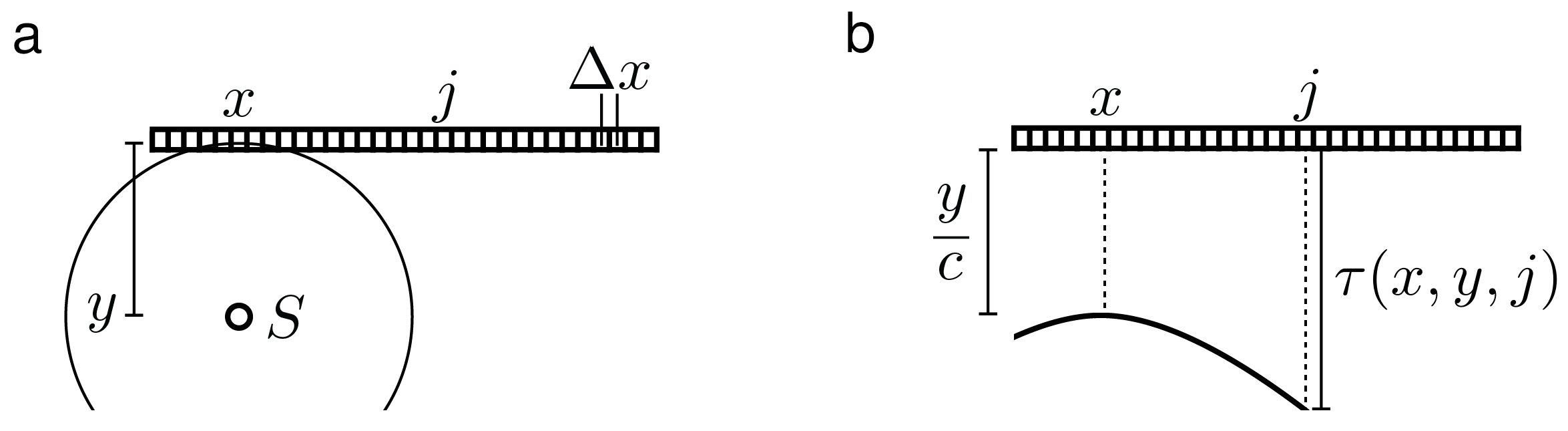
DAS beamforming is the most common and widely used method for reconstructing photoacoustic and ultrasonic images in real-time applications [2,4]. The first step in beamforming an image is to calculate the delays at which a signal originating at some depth y and lateral position x arrives at each of the elements of the transducer. We assume to this end spherical waves coming from the positions we want to reconstruct. Furthermore, we consider a linear transducer consisting of N elements spaced with a distance $\Delta x$ and a spatially constant speed of sound c.

As illustrated in Figure 1, the delay $\tau$ after which a wave originating at lateral position x at a depth y arrives at the element j is:

$$\tau (x,y,j)=\frac{\sqrt{y^2+\left(\right|x-{j·\Delta x\left|\right)}^2}}{c}$$

(1)

The DAS algorithm proceeds by summing up the delayed signals of one position $(x,y)$. We call the signal response measured by transducer element j, at a time $\tau$, $S(j,\tau )$. For a reconstructed pixel at position $(x,y)$, the beamformed signal $S_{\mathrm{DAS}}$ is therefore:

$$S_{\mathrm{DAS}}(x,y)=\sum _{j=1}^{N}S(j,\tau (x,y,j))·A_x\left(j\right)$$

(2)

where $0\le A_x\left(j\right)\le 1$ is an apodization function, which can be used to reduce side lobes and similar beamforming related artifacts, usually by weighting the transducer elements near x stronger than those far away [10].

The complexity of the algorithm can be approximated to be proportional to the number of summations, and is therefore $\mathcal{O}\left(N\right)$ for DAS.

2.2. Delay Multiply and Sum Beamforming

The DMAS algorithm as proposed by Matrone et al. [4] improves on DAS by relating each signal response on each transducer to a single signal position by summing over the products of all non-identical combinations of responses. This has the intention of amplifying actual source signals and reducing noise. To retain linear units, the signed square root of the sums is taken to be the beamformer response. The correlation matrix $M_{nm}(x,y)$ of the signals of the transducer elements n and m, delayed for a signal at lateral position x at depth y, is introduced:

$$M_{nm}(x,y)=S(n,\tau (x,y,n))·A_x\left(n\right)·S(m,\tau (x,y,m))·A_x\left(m\right)$$

(3)

The reconstructed signal $S_{\mathrm{DMAS}}(x,y)$ is then defined as:

$$S_{\mathrm{DMAS}}(x,y)=\sum _{n=1}^{N-1}\sum _{m=n+1}^N\mathrm{sign}\left(M_{nm}(x,y)\right)\sqrt{\left|M_{nm}(x,y)\right|}$$

(4)

While $M_{nm}(x,y)$ is always positive in an ideal tissue and the absence of noise, $\mathrm{sign}\left(M_{nm}(x,y)\right)$ is introduced in the equation to reduce the mean calculated value for noise and artifacts.

The number of summations necessary to determine $S_{\mathrm{DMAS}}$ is $\frac{N^2-N}{2}$. Therefore, in view of N being negligible against $N^2$, computational complexity can be concluded to be $\mathcal{O}\left(N^2\right)$ for DMAS.

2.3. Signed Delay Multiply and Sum Beamforming

In previous DMAS implementations [4], it was necessary to post-process the image after beamforming by using a bandpass filter, as the loss of the sign introduces an additional low frequency component to the actual signal, which is suppressed using the bandpass filter. Unlike in ultrasound imaging, photoacoustic signals usually have a broad acoustic spectrum and therefore contain low acoustic frequencies. These signal contributions will be filtered as well, which may lead to a suppression of important signal components.

In our implementation, we overcome this issue by keeping the sign of the original signal which is equivalent to integrating $\mathrm{sign}\left(S_{\mathrm{DAS}}\right)$ into Equation (4)

$$S_{\mathrm{sDMAS}}(x,y)=\mathrm{sign}\left(S_{\mathrm{DAS}}(x,y)\right)·S_{\mathrm{DMAS}}(x,y)$$

(5)

Keeping the sign of the original signal allows us to apply sDMAS for multispectral PAT application, as shown in the following paragraph.

Here, the number of summations necessary to determine $S_{\mathrm{sDMAS}}$ differs from the case of DMAS only in the N operations for the DAS coefficient; therefore, the number of necessary summations is $\frac{N^2+N}{2}$. Even so, the summations for DAS require far less operations than those for DMAS; either way, we can approximate the complexity of sDMAS to be $\mathcal{O}\left(N^2\right)$, the same as for DMAS.

2.4. Linearity of Beamforming Algorithms

Spectral unmixing of multispectral photoacoustic signals assumes linearity of those signals to the underlying absorption coefficient. While this assumption usually breaks down due to fluence effects, we can still assure that we do not introduce further errors in our estimation through the beamforming algorithm. To show that a beamforming algorithm reconstructs a signal $S_{\mathrm{BF}}(x,y,\lambda )$ linear to the originating signal $S_0(x,y,\lambda )$, we need to show that

$$S_{\mathrm{BF}}(x,y,\lambda )=C(x,y)·S_0(x,y,\lambda )$$

(6)

where $C(x,y)$ has to be a real number, independent of $\lambda$, for any given position $(x,y)$. In the following, we show that this is the case for DAS but not for DMAS, and how we can remedy this by introducing sDMAS.

Whenever a PA signal originating at position $(x,y)$ arrives at transducer element j, the sound wave traveled a distance $d(x,y,j)=c·\tau (x,y,j)$. The signal will have experienced signal attenuation. This acoustic attenuation in a homogeneous medium is $e^{-\alpha \left(\omega \right)d}$, where $\alpha \left(\omega \right)$ is the sound attenuation coefficient dependent on sound frequency $\omega$ and medium. The acoustic signals generated in the tissue during PA image acquisition depend on the optical properties of the tissue and are wavelength dependent. Let $S_0(x,y,\lambda )$ denote the signal that originates as a spherical wave in a sufficiently homogeneous medium at a position $(x,y)$ in response to a laser pulse of wavelength $\lambda$. Then, the resulting attenuated signal $S(j,d(x,y,j),\lambda )$ arriving at transducer element j can be expressed as follows:

$$S(j,d(x,y,j),\lambda )=e^{-\alpha \left(\omega \right)·c·\tau (x,y,j)}·S_0(x,y,\lambda )$$

(7)

In the following paragraphs, we examine the DAS, DMAS and sDMAS algorithms to see how their reconstructions depend on the original signal $S_0$.

2.4.1. Linearity of DAS

From the definition of the DAS beamformed signal (Equation (2)), we directly find linearity for $S_{\mathrm{DAS}}$ after introducing signal attenuation (Equation (7)) and $\lambda$ explicitly.

$$\begin{array}{cc}\hfill S_{\mathrm{DAS}}(x,y,\lambda )& =\sum _{j=1}^N\left(A_x\left(j\right)·e^{-\alpha \left(\omega \right)·c·\tau (x,y,j)}\right)·S_0(x,y,\lambda )\hfill \\ & =C_{\mathrm{DAS}}(x,y)·S_0(x,y,\lambda )\hfill \end{array}$$

(8)

2.4.2. Linearity of DMAS

Using the definition of the DMAS beamformed signal (Equation (4)), we need to consider signal attenuation (Equation (7)) in $M_{nm}(x,y)$, extended for $\lambda$.

$$\begin{array}{cc}\hfill S_{\mathrm{DMAS}}(x,y,\lambda )=& \sum _{n=1}^{N-1}\sum _{m=n+1}^N\mathrm{sign}\left(M_{nm}(x,y,\lambda )\right)\sqrt{\left|M_{nm}(x,y,\lambda )\right|}\hfill \\ \hfill \mathrm{with}{M}_{nm}(x,y,\lambda )=& A_x\left(n\right)A_x\left(m\right)·e^{-\alpha \left(\omega \right)·c·\left(\tau \right(x,y,n)+\tau (x,y,m\left)\right)}·S_0{(x,y,\lambda )}^2\hfill \end{array}$$

(9)

From this expression of $M_{nm}(x,y,\lambda )$m, we see that its sign has to be $+1$, considering $A_x\left(j\right)\ge 0$.

$$\begin{array}{cc}\hfill S_{\mathrm{DMAS}}(x,y,\lambda )=& \sum _{n=1}^{N-1}\sum _{m=n+1}^N\left(\sqrt{A_x\left(n\right)A_x\left(m\right)}·e^{-\frac{1}{2}\alpha \left(\omega \right)·c·(\tau (x,y,n)+\tau (x,y,m))}·\left|S_0(x,y,\lambda )\right|\right)\hfill \\ \hfill =& C_{\mathrm{DMAS}}(x,y)·\left|S_0(x,y,\lambda )\right|\hfill \end{array}$$

(10)

which means that, in DMAS beamforming, we lose the original sign of the signal.

2.4.3. Linearity of sDMAS

We aim to recover this lost sign with sDMAS (Equation (5)) by introducing the sign of $S_{\mathrm{DAS}}$ into DMAS

$$\begin{array}{cc}\hfill S_{\mathrm{sDMAS}}(x,y,\lambda )=& \mathrm{sign}\left(S_{\mathrm{DAS}}(x,y,\lambda )\right)·S_{\mathrm{DMAS}}(x,y,\lambda )\hfill \\ \hfill =& \mathrm{sign}\left(S_{\mathrm{DAS}}(x,y,\lambda )\right)·C_{\mathrm{DMAS}}(x,y)·\left|S_0(x,y,\lambda )\right|\hfill \end{array}$$

(11)

from which we can restore the sign of $S_0$ lost in DMAS, because all other terms in $S_{\mathrm{DAS}}$ (Equation (8)) are positive ($A_x\left(j\right)\ge 0$ and $e^r\ge 0$ because r is a real number).

$$\begin{array}{cc}\hfill S_{\mathrm{sDMAS}}(x,y,\lambda )=& \mathrm{sign}\left(C_{\mathrm{DAS}}(x,y)\right)·C_{\mathrm{DMAS}}(x,y)·\mathrm{sign}\left(S_0(x,y,\lambda )\right)·\left|S_0(x,y,\lambda )\right|\hfill \\ \hfill =& C_{\mathrm{sDMAS}}(x,y)·S_0(x,y,\lambda )\hfill \end{array}$$

(12)

Note that we did not explicitly model noise $N(x,y,\lambda )$ corresponding to the measured signals $S(j,d(x,y,j),\lambda )$ as we assume $S_0(x,y,\lambda )\gg N(x,y,\lambda )$ for the source signals of interest. If the original signal is too small—on a noise equivalent level—linearity cannot be ensured. In the absence of noise, the sign of $S_{\mathrm{DMAS}}$ is always positive for an emerging signal $S_0$, which means that the sign of the original signal is lost through the DMAS double summation process. In contrast, the sign of the original signal is not lost in sDMAS, because we inserted the factor $\mathrm{sign}\left(S_{\mathrm{DAS}}\right)$ thereby eliminating the need for further post-processing with a bandpass filter. Other than that, both beamforming algorithms can be regarded as proportional to the original signal in each beamformed position $(x,y)$. This is regardless of choice in apodization function (as long as $A_x\left(j\right)\ge 0$) but assuming the same acoustic spectrum of the source. For a spectroscopic PA application of DMAS, the acoustic spectrum $\omega$ has to be independent of PA excitation wavelength but can and will depend on the tissue under examination [11].

2.5. Implementation of Beamforming Algorithms

Our implementation of the beamforming algorithms running on a CPU has been multithreaded, but the attainable speed is nevertheless limited. We therefore added implementations of DAS, DMAS and sDMAS using the GPU through the Open Computing Language (OpenCL) [12], which enables us to get increased performance through the massive parallelization of the beamforming algorithms. Delays $\tau (i,j,y)$ for the whole image are computed for a given speed of sound c and up to a maximum scan depth and saved in a persistent GPU buffer. Whenever relevant beamforming parameters change a renewed calculation of the delay buffer is needed. The number of transducer elements which are used for the calculation of a pixel is determined by the sensitive angle, therefore the apodization is also computed beforehand by a separate OpenCL kernel and saved in a persistent buffer. The actual beamforming kernel uses the previously computed buffers to sum over the needed input values according to DAS or sDMAS. In doing so, the main performance limitation is the memory access time on the GPU. Furthermore, we use $A_x\left(j\right)=1,$ for all x and j for the calculation of $\mathrm{sign}\left(S_{\mathrm{DAS}}\right)$, as apodization mainly increases SNR, but the sign of actual signals remains unaffected. Therefore, to reduce computational cost, we refrain here from using an apodization function.

In contrast to the original DMAS formulation, sDMAS does not rely on a bandpass filter as integral part of the beamforming process, which increases performance, as bandpass filters rely on two computationally intensive Fourier transforms. Nevertheless, we provide a bandpass filter as an optional processing step for our implementations of DAS, DMAS and sDMAS as it can reduce noise and artifacts. Our bandpass implementation performs first a Fourier transform of the beamformed image in depth direction using the Fast Fourier Transform (FFT) implementation of the Insight Imaging Toolkit (ITK), then multiplies the resulting image with a Tukey window which can be adjusted to select the desired band of frequencies and gives the option to smoothly set the boundaries of that band to zero [13]. Afterwards, an inverse FFT is applied. The ITK FFT implementation runs on CPU exclusively. Regarding apodization, our MITK implementation supports boxcar, Hanning, and Hamming.

3. Experiments and Results

The purpose of our experiments was to characterize the sDMAS beamforming algorithm in vitro and apply it in vivo for qualitative validation. The first experiment (Section 3.1) characterizes sDMAS beamforming in a controlled in vitro setting and shows both its real-time capability and the linearity. The second experiment (Section 3.2) comprises in vivo measurements on a healthy human volunteer to estimate blood oxygenation (${\mathrm{sO}}_2$) with varying beamformers.

In our setup, raw PA data acquisition is performed using MITK with the DiPhAS US system (Fraunhofer IBMT, St. Ingbert, Germany) and a 128-element linear US transducer operating on a center frequency of 7.5 MHz (L7-Xtech, Vermon, Tours, France). The light from a fast tuning OPO laser (Phocus Mobile, Opotek, Carlsbad, CA, USA) is delivered via a custom fiber bundle to the probe and into the tissue or phantom. A pulse energy of up to 40 mJ at a pulse repetition rate of 20 Hz is delivered over a surface of 2 cm${}^2$ to avoid tissue damage [14]. After the data acquisition, beamforming is performed with the MITK PA image processing plugin [15].

3.1. Beamforming Characterization

The phantom used to characterize the performance of our sDMAS implementation in comparison to DAS and DMAS consists of diluted milk as background medium and a methylene blue solution in silicone tubing with an inner diameter of 1 mm spaced 5 mm apart both vertically and horizontally. To achieve a reduced scattering comparable with tissue (${\mu }_{\mathrm{s}}^{\prime }\approx 15{\mathrm{cm}}^{-1}$ in the near infrared range) [16], the optical properties of concentrated (10% fat) milk and methylene blue were measured by a spectroscopic method [17] and then diluted to yield the desired optical properties, as shown in Figure 2c. The wavelength of the acquisition was varied between 700 and 800 nm to generate PA signals corresponding to a range of absorption coefficients ${\mu }_{\mathrm{a}}$ between 21 and 1.4 cm${}^{-1}$.

Before our characterization experiment, we imaged tubing filled only with water, using the same wavelength sequence to ensure that there was no PA signal contribution by the tubing itself. In these measurements we did not see any PA signal above a noise equivalent level. The characterization phantom was then filled with the diluted methylene blue and measured at a fixed position, as shown in Figure 2a. For each wavelength $n=100$ measurements were performed. Beamforming of raw data from the 128-element transducer was performed to 256 beamformed lines with 2048 samples and up to a depth of 3.8 cm. The speed of sound for that reconstruction was set to 1474 m s${}^{-1}$ as calculated using the corresponding US measurement. Beamforming was performed with with DAS, DMAS and sDMAS using both Hanning and boxcar apodization and with or without a subsequent bandpass filter. When a Tukey bandpass filter was used, it was always applied after beamforming and set to $\alpha =0.5$ with a nominal range from 0 to 10 MHz. B-Mode images were formed by a Hilbert transform based envelope detection and subsequent down-sampling to a $0.15$ mm equal spacing.

A section of the B-Mode images from the phantom which corresponds to ${\mu }_{\mathrm{a}}=8.5$ cm${}^{-1}$ is shown in Figure 3. Bandpass filtered (F) images are shown in the second row. To quantify the improvement in image quality when using sDMAS, we use the Contrast-to-Noise Ratio (CNR) defined as in [18]:

$$\mathrm{CNR}=20·{\log }_{10}\left(\frac{\langle S\rangle -\langle N\rangle }{\sigma \left(N\right)}\right)\mathrm{in}\mathrm{db}$$

(13)

with $\langle S\rangle$ being the mean signal intensity in a region of interest, $\langle N\rangle$ the mean noise intensity and $\sigma \left(N\right)$ the standard deviation of the noise in the adjacent background, as highlighted in Figure 3.

We determine $\langle S\rangle$ from the area highlighted as a white box in Figure 3 and $\langle N\rangle$ as well as $\sigma \left(N\right)$ from the corresponding two black boxes. The increases in CNR using sDMAS over DAS are averaged over $n=100$ and three depths (8, 13 and 18 mm—the three tube sections shown in the figure). As shown in

Table 1. Increase in CNR using sDMAS in different variants (columns) compared to DAS in different variants (rows) in db for ${\mu }_{\mathrm{a}}=8.5{\mathrm{cm}}^{-1}$. Box and Hann denotes if box car or Hanning apodization is compared. F denotes the use of a bandpass filter. For instance, the sDMAS algorithm with boxcar apodization and no bandpass filter (sDMAS, Box, -) on average yielded an improvement of 8 db in CNR over the DAS algorithm with boxcar apodization and using a bandpass filter (DAS, Box, F). CNRs are averaged over $n=100$ slices and three signals in depths of 8 mm to 18 mm. The increases in CNR over the three structures in different depths had standard deviations of 2 db.

			sDMAS
			Box		Hann
			F	−	F	−
DAS	Box	F	9	8	11	9
		−	9	7	11	9
	Hann	F	6	4	8	6
		−	6	5	8	6

, when apodization and bandpass filter are the same for both algorithms, CNR using sDMAS beamforming is consistently at least twice the CNR as when using DAS beamforming (>6 db). In addition, sDMAS improved over DAS regardless of apodization and bandpass for our settings. Sections of B-Mode images with boxcar apodization are shown in Figure 3, which also shows that sDMAS does not suffer from artifacts due to the low frequency term usually introduced in DMAS beamforming. The bandpass filter is therefore an optional step in sDMAS beamforming. The increase in CNR had a depth dependence, with the CNR increasing an average of 1 db more for the structure at 13 mm depth, and having a higher standard deviation at higher depths. In additionl as shown in

Table 2. CNR of DAS, DMAS and sDMAS in db for ${\mu }_{\mathrm{a}}=8.5{\mathrm{cm}}^{-1}$. CNRs are averaged over $n=100$ slices and listed for three signal positions. The CNRs for depths 8 mm and 13 mm had a standard deviation of $\approx 1$ db. For the depth of 18 mm the standard deviation was $\approx 1.5$ db.

	DAS				F-DMAS		sDMAS
	Box		Hann		Box	Hann	Box		Hann
Depth	F	−	F	−			F	−	F	−
8 mm	5	5	8	7	10	11	12	10	14	11
13 mm	4	5	8	7	12	14	14	13	17	15
18 mm	$-3$	$-2$	0	0	6	8	8	6	10	8

, the experiments suggest a $2$ db increase in CNR using F-sDMAS over F-DMAS and a similar CNR when comparing sDMAS to F-DMAS.

The runtimes of the sDMAS and DAS algorithms, as listed in

Table 3. Runtime of our DAS and sDMAS implementations, processing one frame. The standard deviations of the runtimes are each smaller than 5% of the listed means. Choice of apodization had no impact on the runtime. The Tukey window bandpass as well as the B-Mode envelope detection were exclusively performed on CPU.

	DAS		sDMAS		Bandpass	B-Mode
Lines	CPU	GPU	CPU	GPU	CPU	CPU
128	29 ms	6 ms	502 ms	33 ms	9 ms	5 ms
256	58 ms	18 ms	990 ms	63 ms	18 ms	10 ms

, were measured on the characterization phantom dataset with $n=1300$ recorded frames and for a reconstruction depth of 3.9 cm. The reconstruction was performed running MITK on a Ubuntu 18.04 operating system using a i7-5960X CPU (Intel, Santa Clara, CA, USA) and a GeForce GTX 970 GPU (Nvidia, Santa Clara, CA, USA). As the complexity of the DMAS and sDMAS algorithms is the same, the computational performance of DMAS has not been compared to sDMAS and DAS here explicitly.

In Figure 4, we plot the dependence of the signal intensity in the B-Mode images of the beamformed signals on the absorption coefficient of the methylene blue source in the tubing. We did this for the same three tubes as shown in Figure 3 using DAS and sDMAS with a boxcar apodization. A linear fit worked well for the three sources regardless of beamformer. Due to the lower noise level, using sDMAS beamforming, sDMAS has a smaller offset to the x-axis.

3.2. Blood Oxygenation Estimation

To demonstrate the increased quality of blood oxygenation estimation when using sDMAS instead of DAS, we recorded raw PA data of the radial artery and accompanying vein of a healthy human volunteer at five wavelengths in the near infrared. While a good ground truth for blood oxygenation is not easily obtained, in a healthy human, arterial blood is expected to have no less than 90% blood oxygenation [19], which we use as a qualitative reference. Based on the work of Luke et al. [20] and considering the power spectrum of our laser source, we altered our wavelength sequence from an equidistant spacing towards wavelengths with optimal differences between absorption of oxygenated and deoxygenated hemoglobin. The acquisition wavelength sequence was measured by a spectrometer (HR2000+, Ocean Optics, Dunedin, New Zealand) as $(722,756,831,907,943)$ nm with an accuracy of $1.5$ nm. The acquired raw PA data were corrected for fluctuations in laser pulse energy and then beamformed using the DAS and sDMAS beamforming algorithms.

Spectral unmixing was performed using the non-negative constrained least squares solver scipy.optimize.nnls [21] on sets of five beamformed images, yielding abundances for hemoglobin and deoxygenated hemoglobin by fitting the spectra of the two chromophores to the five measured wavelengths in each pixel. The unmixing algorithm was implemented for CPU only, as its performance was not critical. Figure 5 shows a F-DAS and F-sDMAS beamformed example image recorded at an excitation wavelength of 831 nm. Sections of the radial artery and accompanying vein were identified by a vascular surgeon in the US image live stream of the acquisition system. The unmixing results for oxygenated (${\mathrm{HbO}}_2$) and deoxygenated hemoglobin (Hb) were used to calculate blood oxygenation and total hemoglobin (THb):

$${\mathrm{sO}}_2=\frac{{\mathrm{HbO}}_2}{\mathrm{Hb}+{\mathrm{HbO}}_2},\mathrm{THb}=\mathrm{Hb}+{\mathrm{HbO}}_2.$$

(14)

${\mathrm{sO}}_2$ is visualized by masking the results for low values of $\mathrm{THb}$.

The median blood oxygenations ${\mathrm{sO}}_2$ were averaged over $n=84$ beamformed B-Mode images for both F-DAS and F-sDMAS. Using F-DAS, this yielded an estimation of arterial blood oxygenation ${\mathrm{S}}_{\mathrm{a}}{\mathrm{O}}_2^{\mathrm{DAS}}=71\%\pm 6\%$ while the same unmixing on F-sDMAS yielded ${\mathrm{S}}_{\mathrm{a}}{\mathrm{O}}_2^{\mathrm{sDMAS}}=89\pm 6\%$. The estimation of venous blood oxygenation yielded ${\mathrm{S}}_{\mathrm{v}}{\mathrm{O}}_2^{\mathrm{DAS}}=44\%\pm 7\%$ and ${\mathrm{S}}_{\mathrm{v}}{\mathrm{O}}_2^{\mathrm{sDMAS}}=37\pm 8\%$.

4. Discussion

We presented a variant of the (F-)DMAS algorithm termed sDMAS that preserves linearity in the original signal response while increasing image quality. We implemented the sDMAS algorithm within MITK to be easily accessible and open-source to be easily reproducible and to address the lack of such resources in the field. A user manual for the software can be found here http://docs.mitk.org/nightly and demo installation packages with a sample of the raw data here http://mitk.org/wiki/Photoacoustics. We also provide reference DAS, DMAS implementations and bandpass filtering and include envelope detection algorithms for B-Mode imaging. Our results clearly show that our implementation is real-time capable (for frame rates of 20 Hz at which our imaging system operates), although there is a limit for the achievable image resolution when using consumer GPUs, as we did. Image quality was clearly improved using (F-)sDMAS compared to (F-)DAS. Due to this increase in CNR, we could also show that sDMAS B-Mode images are not only linear to the absorption coefficient of a source but also have a lower noise component than DAS, which systematically skews the spectral unmixing of DAS beamformed images more than for DMAS. This is finally illustrated in vivo on a healthy human volunteer’s radial artery and accompanying vein. Although we are missing a reliable reference measurement, the spectral unmixing results of the arterial blood oxygenation for sDMAS ($89\%$) are in closer agreement with the literature [19] than the ${\mathrm{S}}_{\mathrm{a}}{\mathrm{O}}_2$ values using F-DAS, which estimated it as $71\%$, which is definitely too low for a healthy human. While this suggests that sDMAS results are more easily quantified in functional terms and can more accurately estimate quantities such as blood oxygenation, it is far from conclusive and, as it is only a qualitative result, further research is needed. The reconstructed images still contain artifacts and noise that might be reduced further using other beamforming methods such as Minimum Variance (MV) beamforming [10], Double stage DMAS [3] or further modifications of DMAS such as the introduction of MV into DMAS [22]. They are however non-linear and computationally expensive. Therefore, they are currently not usable for real-time multispectral applications. However, further study of those methods and appropriate extensions and implementations might give insight into their applicability to multispectral PA imaging. Other issues such as wavelength dependent fluence effects [23], or limited views of PA sensor arrays cannot be solved by a beamforming algorithm alone and will impact functional PA imaging independent of the beamformer.

In conclusion, the presented sDMAS algorithm offers a superior image quality compared to DAS and preserves linearity in the original signal on the same level as DAS, which makes it suitable for spectroscopic PA applications. Furthermore, sDMAS can be performed in real-time and is as such usable in a clinical setting.

References

- Griffiths, L.; Jim, C. An alternative approach to linearly constrained adaptive beamforming. IEEE Trans. Antennas Propag. 1982, 30, 27–34. [Google Scholar] [CrossRef]
- Kim, J.; Park, S.; Jung, Y.; Chang, S.; Park, J.; Zhang, Y.; Lovell, J.F.; Kim, C. Programmable real-time clinical photoacoustic and ultrasound imaging system. Sci. Rep. 2016, 6. [Google Scholar] [CrossRef] [PubMed]
- Mozaffarzadeh, M.; Mahloojifar, A.; Orooji, M.; Adabi, S.; Nasiriavanaki, M. Double Stage Delay Multiply and Sum Beamforming Algorithm: Application to Linear-Array Photoacoustic Imaging. IEEE Trans. Biomed. Eng. 2017, 65, 31–42. [Google Scholar] [CrossRef] [PubMed]
- Matrone, G.; Savoia, A.S.; Caliano, G.; Magenes, G. The Delay Multiply and Sum Beamforming Algorithm in Ultrasound B-Mode Medical Imaging. IEEE Trans. Med. Imag. 2015, 34, 940–949. [Google Scholar] [CrossRef] [PubMed]
- Park, J.; Jeon, S.; Meng, J.; Song, L.; Lee, J.S.; Kim, C. Delay-multiply-and-sum-based synthetic aperture focusing in photoacoustic microscopy. J. Biomed. Opt. 2016, 21. [Google Scholar] [CrossRef] [PubMed]
- Matrone, G.; Ramalli, A.; Savoia, A.S.; Tortoli, P.; Magenes, G. High Frame-Rate, High Resolution Ultrasound Imaging with Multi-Line Transmission and Filtered-Delay Multiply and Sum Beamforming. IEEE Trans. Med. Imag. 2017, 36, 478–486. [Google Scholar] [CrossRef] [PubMed]
- Alshaya, A.; Harput, S.; Moubark, A.M.; Cowell, D.M.; McLaughlan, J.; Freear, S. Spatial resolution and contrast enhancement in photoacoustic imaging with filter delay multiply and sum beamforming technique. In Proceedings of the 2016 IEEE International Ultrasonics Symposium (IUS), Tours, France, 18–21 September 2016; pp. 1–4. [Google Scholar]
- Treeby, B.E.; Zhang, E.Z.; Cox, B.T. Photoacoustic tomography in absorbing acoustic media using time reversal. Inverse Prob. 2010, 26. [Google Scholar] [CrossRef]
- Nolden, M.; Zelzer, S.; Seitel, A.; Wald, D.; Müller, M.; Franz, A.M.; Maleike, D.; Fangerau, M.; Baumhauer, M.; Maier-Hein, L.; et al. The Medical Imaging Interaction Toolkit: Challenges and advances. Int. J. Comput. Assist. Radiol. Surg. 2013, 8, 607–620. [Google Scholar] [CrossRef] [PubMed]
- Holfort, I.K.; Gran, F.; Jensen, J.A. Broadband minimum variance beamforming for ultrasound imaging. IEEE Trans. Ultrason. Ferroelectr. Freq. Control 2009, 56, 314–325. [Google Scholar] [CrossRef] [PubMed] [Green Version]
- Xu, G.; Dar, I.A.; Tao, C.; Liu, X.; Deng, C.X.; Wang, X. Photoacoustic spectrum analysis for microstructure characterization in biological tissue: A feasibility study. Appl. Phys. Lett. 2012, 101. [Google Scholar] [CrossRef] [PubMed]
- Tompson, J.; Schlachter, K. An introduction to the opencl programming model. Pers. Educ. 2012, 49, 777–780. [Google Scholar]
- Harris, F.J. On the use of windows for harmonic analysis with the discrete Fourier transform. Proc. IEEE 1978, 66, 51–83. [Google Scholar] [CrossRef] [Green Version]
- Laser Institute of America. American National Standard for Safe Use of Lasers; Laser Institute of America: Orlando, FL, USA, 2007. [Google Scholar]
- Kirchner, T.; Sattler, F.; Dinkelacker, S.; Goch, C.J.; Gröhl, J.; Nolden, M.; Maier-Hein, L. MITK/MITK: sDMAS-2018.07. 2018. Available online: https://zenodo.org/record/1303376#.W7_9blL3McU (accessed on 11 September 2018). [CrossRef]
- Jacques, S.L. Optical properties of biological tissues: A review. Phys. Med. Biol. 2013, 58. [Google Scholar] [CrossRef]
- Flock, S.T.; Jacques, S.L.; Wilson, B.C.; Star, W.M.; van Gemert, M.J.C. Optical properties of intralipid: A phantom medium for light propagation studies. Lasers Surg. Med. 1992, 12, 510–519. [Google Scholar] [CrossRef] [PubMed]
- Welvaert, M.; Rosseel, Y. On the Definition of Signal-To-Noise Ratio and Contrast-To-Noise Ratio for fMRI Data. PLoS ONE 2013, 8, 1–10. [Google Scholar] [CrossRef] [PubMed] [Green Version]
- Zander, R. The oxygen status of arterial human blood. Scand. J. Clin. Lab. Investig. 1990, 50, 187–196. [Google Scholar] [CrossRef]
- Luke, G.P.; Nam, S.Y.; Emelianov, S.Y. Optical wavelength selection for improved spectroscopic photoacoustic imaging. Photoacoustics 2013, 1, 36–42. [Google Scholar] [CrossRef] [PubMed]
- Lawson, C.L.; Hanson, R.J. Solving Least Squares Problems; SIAM: Bangkok, Thailand, 1995. [Google Scholar]
- Mozaffarzadeh, M.; Mahloojifar, A.; Orooji, M.; Kratkiewicz, K.; Adabi, S.; Nasiriavanaki, M. Linear-array photoacoustic imaging using minimum variance-based delay multiply and sum adaptive beamforming algorithm. J. Biomed. Opt. 2018, 23. [Google Scholar] [CrossRef] [PubMed]
- Kirchner, T.; Gröhl, J.; Maier-Hein, L. Context encoding enables machine learning-based quantitative photoacoustics. J. Biomed. Opt. 2018, 23, 056008. [Google Scholar] [CrossRef] [PubMed] [Green Version]
Figure 1.
(a) Illustration of a signal S originating at depth y and lateral position x relative to a transducer array with example element j and propagating as a spherical acoustic wave with speed c; (b) Illustration of the same scenario in the time domain of pressure recorded in the transducer array (radio frequency (rf) data), where denotes the propagation time of that signal S.
Figure 2.
The characterization phantom, consisting of (a) an array of silicone tubing filled with diluted methylene blue and placed inside (b) a tank filled with diluted milk. (c) The methylene blue in the tubing was diluted to yield absorption coefficients as encountered in blood in the near infrared range (the overlaid dots are the wavelengths of the acquisition sequences). The milk was diluted to yield a reduced scattering coefficient consistent with tissue.
Figure 3.
Visualization of B-Mode PA images with logarithmic compression using DAS, DMAS and sDMAS beamforming in the first row, with an additional bandpass filter (F) applied in the second row. The PA signals from the upper and lower boundaries of the tubes are visible with a distance of 1 mm. For the purpose of ascertaining a CNR ratio as defined in Equation (13), the white box indicates the signal S and the black boxes the corresponding noise N. These regions are identical for all algorithms. The images shown are a representative example, beamformed using a boxcar apodization using an acquisition wavelength corresponding to an absorption coefficient of cm inside the tubing.
Figure 4.
Comparison of the signal intensities dependence on the absorption coefficient. The maximum signal intensities in B-Mode images beamformed with DAS and sDMAS using boxcar apodization are averaged over images for three sources. Linear fits are plotted alongside with the measured data. Both DAS and sDMAS have a proportional relation to the sources absorption coefficient when accounting for an additive noise term.
Figure 5.
The radial artery and accompanying vein of a healthy human volunteer. Representative B-Mode images recorded at an acquisition wavelength of 831 nm are shown in the top row. Beamforming was performed using Hanning apodization and the images where postprocessed with a bandpass filter (F). In the second row, blood oxygenation () is visualized. Only values with high total hemoglobin as determined by the spectral unmixing are shown. The dashed green box marks the artery and the dotted line the accompanying vein as identified by a consulting physician; both are annotated with the median oxygenation within these boxes.