The Ascendency of Numerical Methods in Lens Design


Optical Systems Design, Inc., East Boothbay, ME 04544, USA
J. Imaging 2018, 4(12), 137; https://doi.org/10.3390/jimaging4120137
Submission received: 23 October 2018
/
Revised: 19 November 2018
/
Accepted: 19 November 2018
/
Published: 24 November 2018
(This article belongs to the Special Issue Computation and Analysis of Imaging Aberrations)
Abstract
:Advancement in physics often results from analyzing numerical data and then creating a theoretical model that can explain and predict those data. In the field of lens design, the reverse is true: longstanding theoretical understanding is being overtaken by more powerful numerical methods.
1. Introduction
As a student, walking through the halls of the physics department at the Massachusetts Institute of Technology (MIT), I saw a sign on a door that read “Numerical Methods”. On a table were stacks of computer printouts, the products of early batch-mode mainframes. I learned they were calculations of nuclear cross sections, tables of numbers filling whole pages, the stacks about a foot high. “Who is ever going to read those printouts?” I wondered. I suspect that the physics is better understood now, and a theoretical approach can answer the questions they were then investigating numerically. In that field, theory has likely replaced number crunching. What about in the field of optics?
Today, as I examine any of the textbooks on lens design [1,2,3,4,5,6,7] I see pages of mathematics and ask, “Who is ever going to read all those equations?” And what good would it do if they did?
This brings up a fundamental question: Should one read them, study them for a lifetime and become so expert that the solution to a lens design problem can be predicted by exercising that knowledge? This was the practice of many experts of the past and is still a widely held view today; but is it valid?
Recent developments suggest otherwise. It is now possible to simply enter the requirements into a powerful computer program (Appendix A) and in a matter of minutes obtain a design that is considerably better than those produced by the experts of an older generation. This fact makes some people uncomfortable, as well it should—but one must embrace the technology of today and not get distracted by nostalgia for an earlier era.
The underlying problem in lens design is to find an arrangement of lens elements that yields an image in an accessible location with the required degree of resolution, transmission, and so on. Reduced to basics, there are two overriding questions: Is the image sharp, and is it in the right place? Calculating the answers to these questions numerically has historically been so labor intensive that recourse to theory often seemed justified. That is less true today.
I note that studying the classic texts is still worthwhile however—although not for the mathematics. There is a whole lot of practical knowledge there, advice on material selection, mounting, tolerances, and more—topics that every practicing lens designer should be familiar with. The computer cannot decide broad issues of this nature, and you must still come up with a first-order solution before you can send those data to the computer. The rest can be left to the machine.
2. Theory vs. Number Crunching
There have long been two schools of lens design, theorists and number crunchers [8]. Even the old masters were at odds on this issue. In Germany, we find luminaries like Petzval (1807–1891) and Abbe (1840–1905) who insisted that a design must be finalized by numerical ray tracing, however laborious, before anyone touched a piece of glass. The job could take months of calculations by a team of assistants. In England on the other hand, Hastings (1848–1932) and Taylor (1862–1943) applied theoretical tools, namely third-order Seidel theory, to devise a lens prescription analytically, fully aware that the result was only a crude approximation of what they were after. Then they would grind and polish that third-order design, measure the image errors, and iterate. That effort also required much time. (I note that the polished lens was in effect an excellent analog computer, capable of tracing rays at the speed of light. In today’s terms, it was the programming of that computer that took so much time.) Each school thought the other misguided.
Today, lens design software invariably attempts to minimize a merit function (MF), which is usually defined as the sum of the squares of a set of defects of various types. These may include image blur size, distortion, and whatever mechanical properties one would like to control in a particular way. Once the MF is suitably defined, finding a design with the lowest practical value becomes an exercise in number crunching, with the mathematics built into the software.
The authors of recent textbooks on lens design invariably instruct the reader to first work up a third-order solution by hand before submitting it to computer optimization. Even that idea is also now obsolete, in my opinion.
3. Classical Attempts
It is instructive to page through some of those textbooks, where one finds passages yielding insights into how a certain aberration can be reduced by a certain type or combination of elements, with examples and theory to prove it. But there is a serious shortcoming to that approach: Granted that a particular insight might be fruitful when applied to a given problem, one would also like the process to work for other problems, and each requires its own insight. Even the best masters in the field cannot master so broad a field.
The culmination of this theoretical approach is found in a classic text by Cox [9], where one finds over 600 pages of dense algebra. In sympathy with the author, who was trying to develop a theory sufficiently better than the third-order to be comprehensive, one must admire the result, an opus that is a monument to human dedication. But I submit that nobody is going to wade through 600 pages of algebra when they want to design a lens. In short, I argue that the theoretical approach has collapsed under its own weight. One simply cannot, in spite of generations of mathematical genius, design lenses according to a set of algebraic statements. So where are we now?
4. Modern Developments
Perhaps the Germans were right all along, only the technology was lacking. Imagine tracing hundreds or thousands of rays with log tables, or a Marchand calculator! The labor required was staggering. I quote Kingslake (1903–2003):
“…nobody ever traced a skew ray before about 1950 except as a kind of tour-de-force to prove that it was possible…”
“When someone applied for a position in our department at Kodak, I would ask him if he could contemplate pressing the buttons of a desk calculator for the next 40 years, and if he said ‘yes’, I would hire him.”
Can anything be done to relieve the tedium, to make lens design a practical endeavor, attractive to today’s students, accustomed to instant gratification on their smart phones? That has been my goal during the 50 years I have worked on the problem.
The result of this labor seems to be a resounding success, and it shows the power of number crunching, as I will describe below. I attribute the success of this new paradigm to two developments:
- development of the PSD III algorithm for minimizing a merit function; and,
- a binary search technique applied to global optimization.
The PSD III algorithm [10] is an improvement over the classic damped-least-squares (DLS) method of minimizing a merit function. The mathematics of that method is quite simple. It involves finding the derivatives of every operand in the merit function (a score whose value would be zero if the lens were perfect) with respect to the design variables (radii, thicknesses, etc.), and then solving for the set of variables that reduces the value of that MF. A linear solution would be simple to calculate but wildly inaccurate since the problem is very nonlinear. Therefore, a “damping factor”, D, is added to the diagonal of the Jacobian matrix used to calculate the change vector, reducing the magnitude of the latter and (one hopes) keeping it within the region of approximate linearity; then iterating, over and over. Although it works, this method is often painfully slow.
Instead, the PSD III method anticipates the effect of higher-order derivatives by comparing the first derivatives from one iteration to the next. This process assigns a different value of D to each variable, as explained in Reference [10].
The results are stunning. Whereas classic DLS applies the same D to each variable, the PSD III method finds values that differ, from one variable to the next, by as much as 14 orders of magnitude. Clearly, DLS is a very poor approximation to that result, which accounts for its very slow convergence.
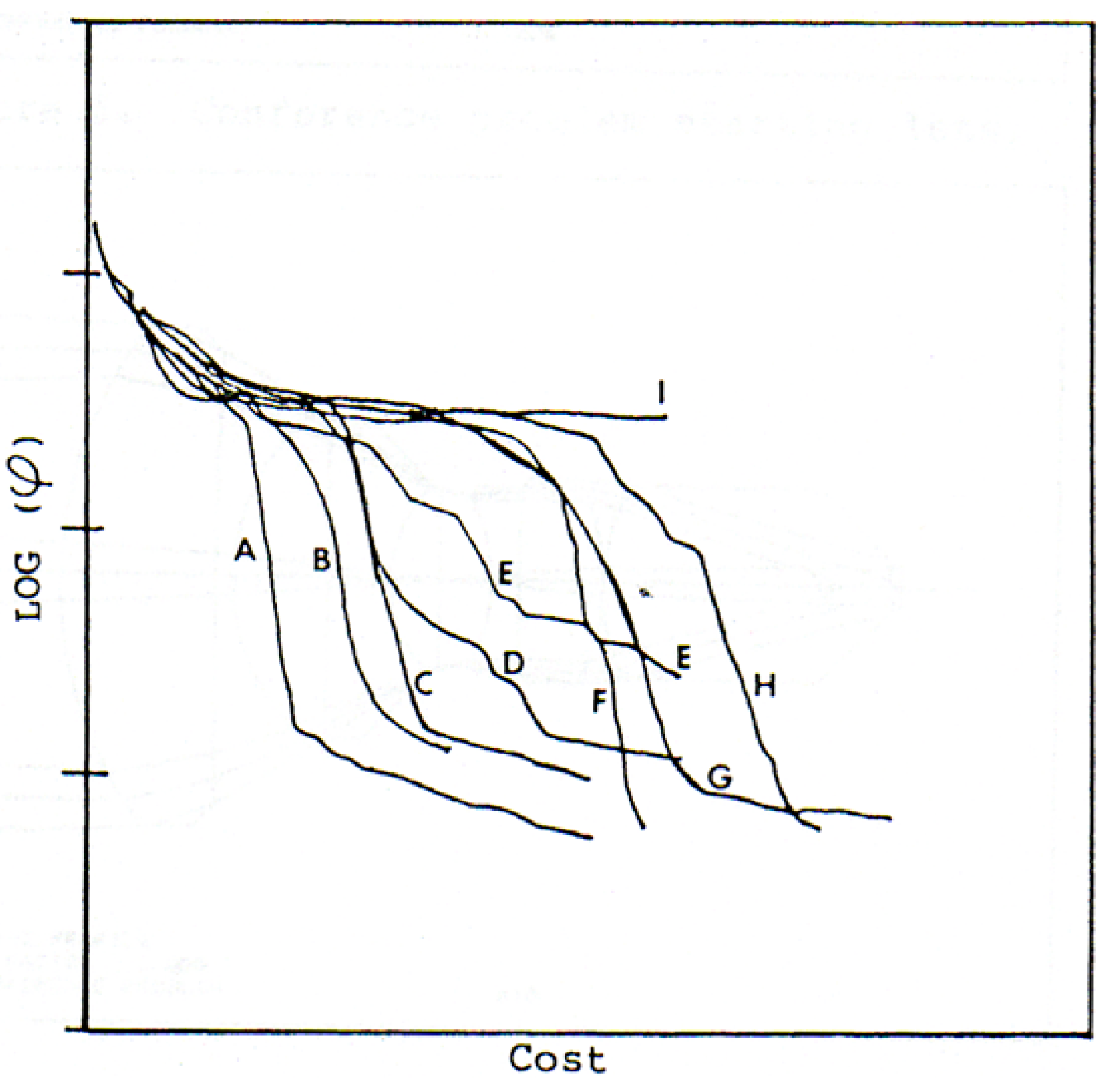
Figure 1 shows a comparison of the convergence rates of several optimization algorithms when designing a triplet lens. The PSD III method is in curve A, and curve I is DLS. (The other curves refer to other algorithms that have been tested [11]). The merit function is given by φ, and the cost is the elapsed time to get that value. Few technical fields experience an improvement of this magnitude at one stroke. I am still amazed by the results.
This figure shows that, for the DLS method (curve I), achieving a low value of the MF (which would be lower on the plot) one must go a great distance to the right, since that curve has a very small slope. That translates into a great deal of time spent making countless very small improvements. For years, that slow rate of convergence has been the bottleneck of the whole industry. The PSD III method has broken that bottleneck.
5. Global Optimization
Much effort has been expended by the industry on so-called “global optimization” methods. In principle, the approach can be very simple: make a mesh of nodes, where every radius, thickness, and so on takes on each of a set of values in turn, and optimize each case. Some designers report evaluating a network of perhaps 200,000 nodes and, given an infinite amount of time, this approach can indeed find the best of all lens constructions, but we can do better.
The second development that contributes to the success of this new paradigm is the binary search method used to find the optimum solution [12]. This concept models the lens design landscape as a mountain range, with peaks and valleys all over the place. The best lens solution is in the lowest valley. So how do you find it? If you are in a valley, you cannot see if there is a lower one somewhere else.
But if you are at the top of the highest mountain, you can see all the valleys in the area, and that is the clue we need. The mountaintop corresponds to a lens with all plane-parallel surfaces. The binary search algorithm then assigns a weak power to each element according to a binary number, where 0 is a negative element and 1 is positive. By examining all values of that binary number, one examines all combinations of element powers. The only quantities still to be defined are what that power should be and what thicknesses and airspaces to assign to the elements; those are input parameters to the algorithm. With this method, a five-element lens has only 32 combinations of powers, which is far more tractable than evaluating 200,000, and the results are gratifying.
(We note that this is actually an old idea. Brixner [13] applied this logic a generation ago, running very long jobs on a mainframe computer. He was on the right track, but computer technology was not up to the task, and optimization was still DLS.)
Let us examine the results of applying this algorithm to some classical lens constructions and compare the results with what was accomplished by yesterday’s experts.
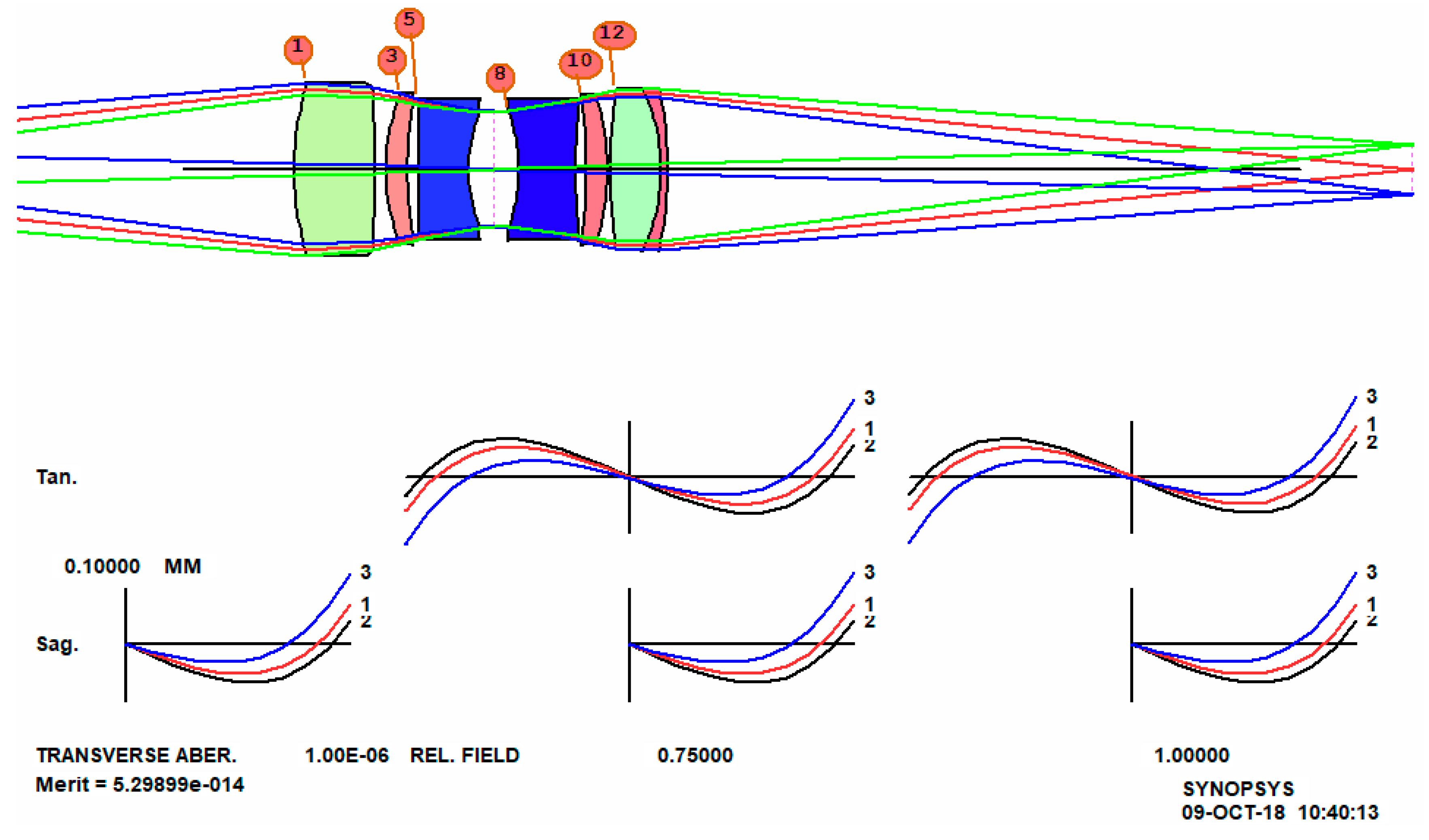
5.1. Unity-Magnification Double-Gauss
This is a classic design, the example taken from Kingslake and Johnson [1] (p. 372), shown in Figure 2. Let us see what our new algorithm can do on this problem. We will use a feature called Design SEARCH (DSEARCH), an option in the SYNthesis of Optical SYStems (SYNOPSYS) program. Here is the input (Appendix B):
In the above input file, we first define the system parameters, object coordinates, wavelengths, and units. Then the GOALS section specifies the number of elements, first-order targets, and fields to correct, asks for an annealing stage, and directs the program to use the quick mode. This mode runs two optimizations on the candidates, the first with a very simple MF consisting of third- and fifth-order aberrations plus three real rays. This executes very quickly, since little ray tracing is involved. The winners of this stage are then subjected to a rigorous optimization, with grids of real rays at the requested fields (0.0, 0.75, and 1.0). The SPECIAL AANT section defines additional entries we wish to go into the MF, in this case controlling edge and center thicknesses and requiring the Gaussian image height to equal the object height, with a sign change. That gives us the desired 1:1 imaging.
In these examples, we elect to correct image errors by reducing the geometric size of the spot at each field point. The software can also reduce optical path difference errors (OPD), a feature useful for lenses whose performance must be close to the diffraction limit, and it can even control the difference in the OPD at separated points in the entrance pupil, which has the effect of maximizing the diffraction MTF at a given spatial frequency. As computer technology advances, the software keeps pace, adding new features as new possibilities are developed.
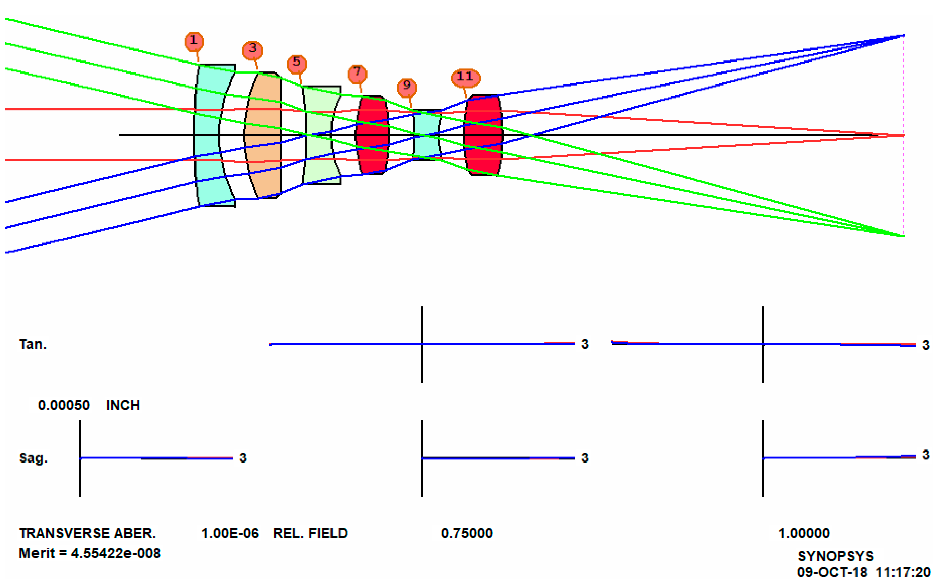
This job runs in 87.7 s, on our 8-core hyperthreaded PC, and the results are shown in Figure 3.
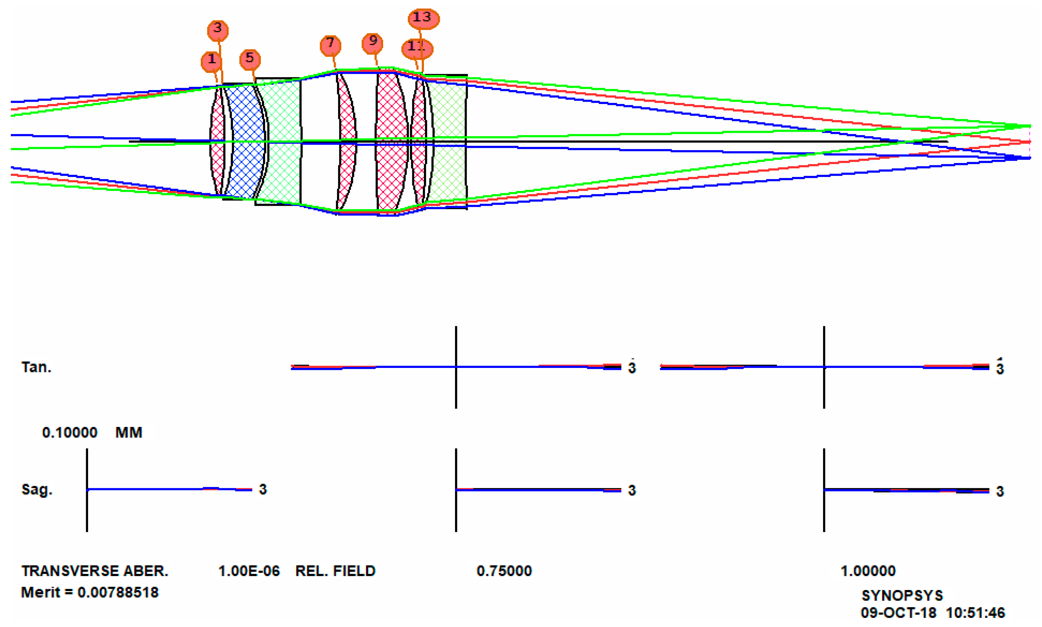
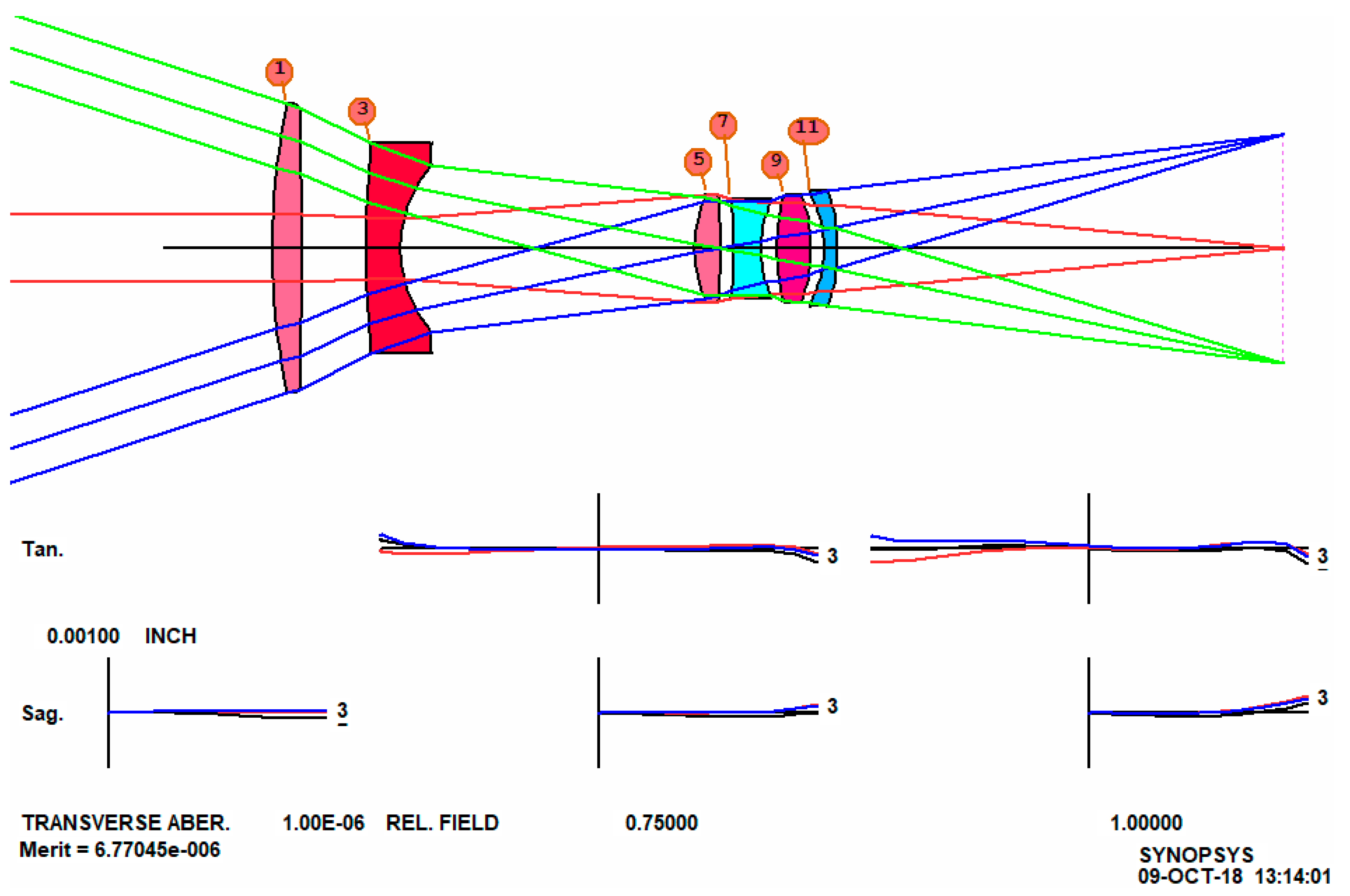
The cross-hatch pattern indicates that the design at this stage uses model glasses, and the next step is to replace them with real ones. We run an optimization MACro that DSEARCH has created, and then run the Automatic Real GLASS option (ARGLASS), specifying the Schott catalog. The result, after about 30 s more, is shown in Figure 4. Clearly, this design is vastly better than the classic version, even though it does not resemble the double-Gauss form anymore. In less than two minutes, we have a design far better than what an expert could produce using profound theoretical knowledge a generation ago.
An interesting feature of these new tools arises from the annealing stage of optimization, a process that alters the design parameters by a small amount and reoptimizes, over and over. Due to the chaotic nature of the lens design landscape, any small change in the initial conditions sends the program to a different solution region. Therefore, if we run the same job again, with the same input, we often get a rather different lens. Usually the quality is about the same, and if we run it several times, we get a choice of solutions. This too is an improvement over classical methods, since once the old masters succeeded in obtaining a satisfactory design, it is unlikely they would start over and try to find an even better one. However, now we can easily evaluate several excellent lenses and select the one we like best. Chaos in lens design is discussed more fully by Dilworth [14].
5.2. Six-Element Camera Lens
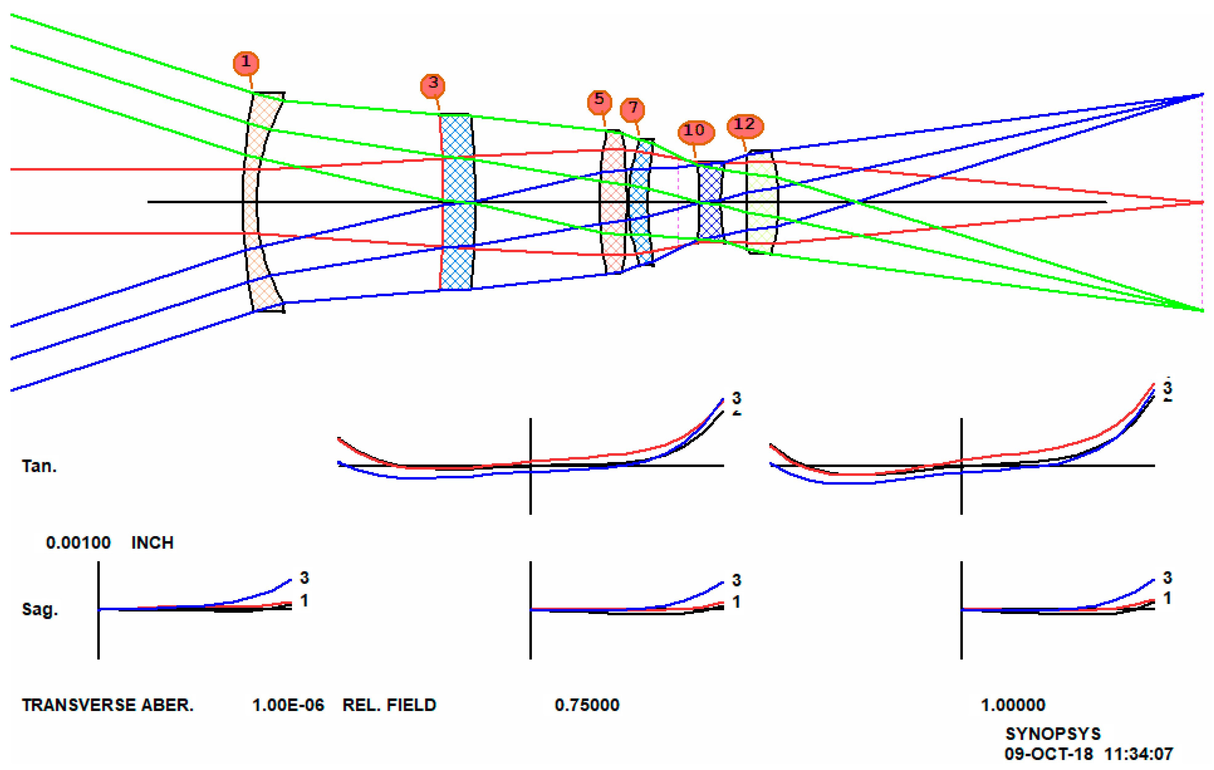
Our second example is taken from Cox, number 3-87, patent number 2892381, shown in Figure 5. This is an excellent design, with about one wave of lateral color. (We have used model glasses here, since the reference does not give the glass types and there are no catalog glasses with just those values.)
This looks like a more difficult problem. What can DSEARCH do with this one? Here is the input file (Appendix C).
The result, with real glass, is shown in Figure 6. Again, it does not resemble the classic form, but is far superior. There is a lesson there; the old masters often started with a well-known form, in this case the triplet, hoping its symmetry would yield some advantage for correcting aberrations. However, it is not likely they would have thought of the configuration found by DSEARCH. We were able to get these results in just over one minute by pure number crunching. We suspect that the original designer (Baker) invested far more time—and would probably be very impressed with these new results.
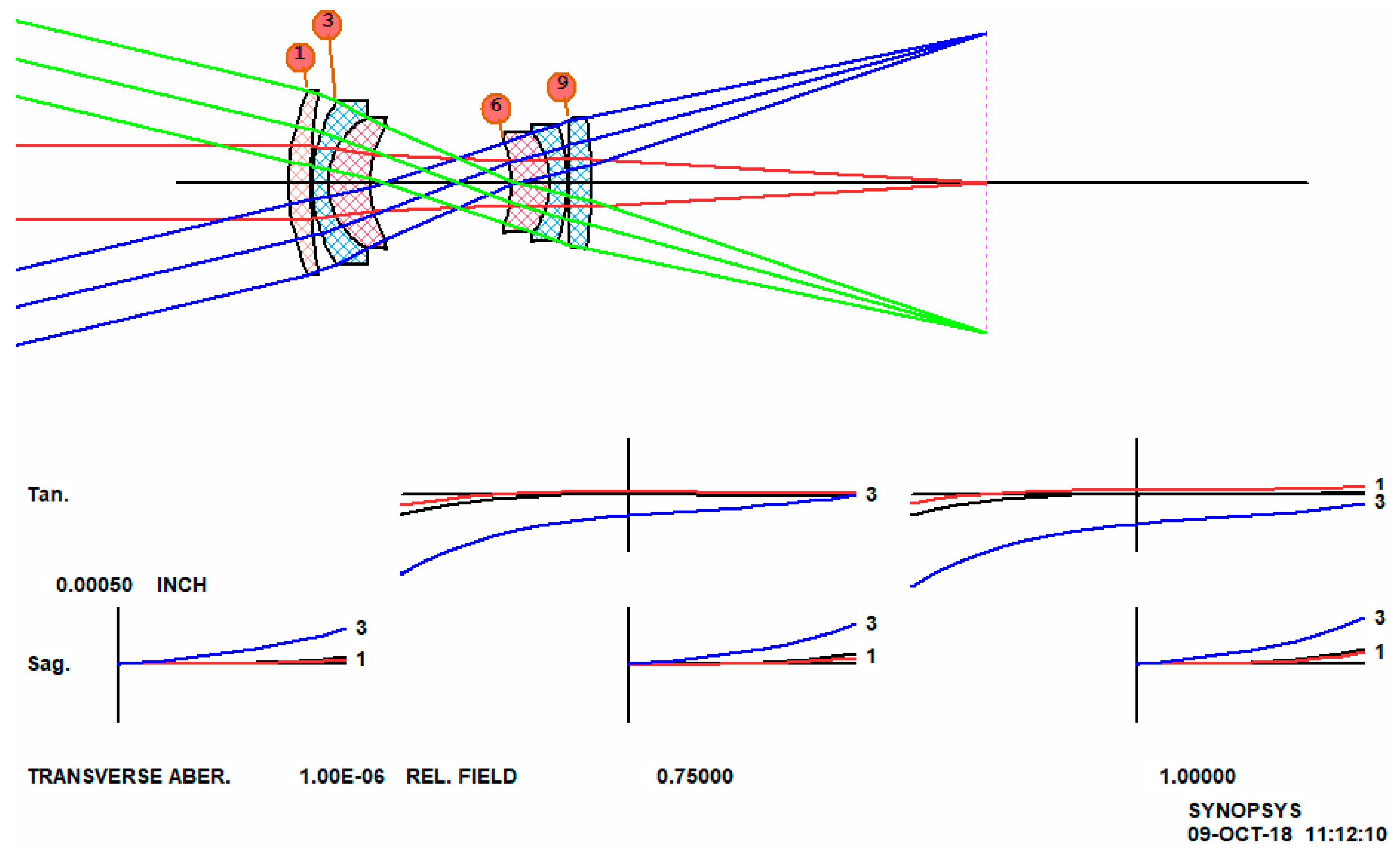
5.3. Inverse Telephoto Lens
This example is also taken from Cox, number 7—14, patent 2959100. It is a reasonably good design, as shown in Figure 7. The input for DSEARCH has an extra requirement in the SPECIAL AANT section, since the lens was designed for low distortion and we want to control that as well (Appendix D).
DSEARCH returns the lens in Figure 8, also better than the patented lens designed by an expert.
Once again, we see that numerical methods are far superior to the best that an expert designer could do a generation ago.
But wait, suppose we decide those elements are too thick. The solution is simple, just change the ACC monitor (automatic center-thickness control) in the SPECIAL AANT section so they stay below 0.1 inches, as in the patent, and run the job again. The result is almost identical, except the elements are thinner. The program has options to control almost anything in the lens, a vital requirement for when one is addressing a problem with numerical methods.
5.4. Other Methods
We have shown how the design search algorithm (DSEARCH) can find solutions better and faster than can a human expert, even those with a lifetime of experience. But it is not the only new technique that replaces theory with number crunching.
Let us try running the last example with a different feature [15], one that employs an idea originally by Bociort [16] called the saddle-point method. This method does not use either a grid of designs or a binary search. Instead, it modifies an existing lens by adding a thin shell at a selected surface. The shell does not change the paths of rays but adds six new degrees of freedom. The program tries every surface within a specified range and optimizes each attempt. Then it selects the best and begins again, adding a new element to that design, and so on until the desired number of elements is reached.
Here is the input for SPBUILD (saddle-point build) (Appendix E):
In a few minutes this input returns the lens in Figure 9, fitted with real glass as before.
Here is yet another way to employ number crunching to explore the design space. Note that neither this method nor the binary search method of DSEARCH uses any of the classic theoretical tools. The work is done via numerical methods alone, since the laws of optics have been encoded in the software.
Although the saddle-point method can build up an entire lens from nothing, as we have seen, it is most useful when one already has a design that is close to the desired goals and would like to find the best place to insert an additional element. At this point, an expert would likely look at how the third-order aberrations build up through the lens and using his deep knowledge of theory would try to predict the optimum location. But another feature does the same job much better and faster than can a human, no matter how skillful. This also uses the saddle-point concept and an example will be shown in the next section.
5.5. Zoom Lenses
Thus far, these examples have all been fixed-focus lenses. Can number crunching also produce quality zoom lenses?
The question came up when a colleague sent me nine pages of hand calculations for a zoom lens. He was using classical methods and knew what he was doing—but I viewed this as another case where it would be nice to make the computer do all the work. The result was a feature called ZSEARCH [17]. The example below shows that although number crunching does the lion’s share of the work, a skillful human designer still has an important role to play.
We will design a 13-element zoom lens with a 30:1 zoom ratio. Not an easy job, especially since, as with the previous examples, we do not give the program any starting design. To speed things up, we start with 11 elements, which means there are 2048 cases to analyze utilizing the binary search method. This of course takes much longer than the previous examples—but it is still much faster than doing the work by hand. This will be the input for ZSEARCH (Appendix F):
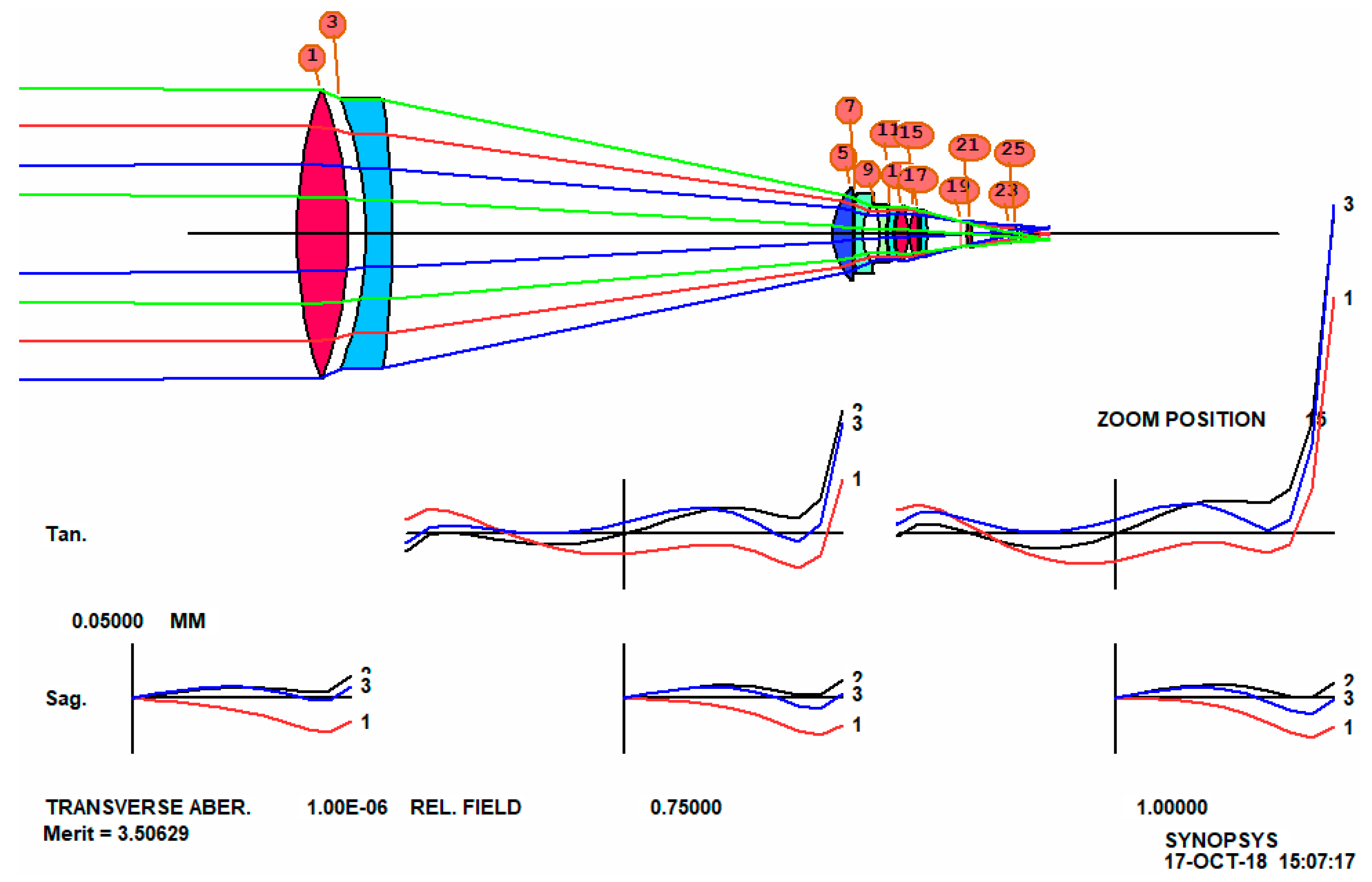
This runs for about 26 min and produces a lens that is tolerably well corrected at all seven of the zoom positions we requested, as shown in Figure 10. Now we will improve this lens.
When we examine the performance over 100 zooms, things are not so good, and there are overlapping elements in one place, which is not surprising for so wide a range and so few zooms corrected. However, there are tools for these problems too. We ask the program to define 15 zoom positions.
CAM 15 SET
And then reoptimize and anneal. Now the lens is much better, but some elements are too thin at the center or edge, and we need yet more clearance between zoom groups. We modify the MF requirements to better control center and edge clearances, and also declare the stop surface a real stop, so the program finds the real chief ray by iteration (instead of using the default paraxial pupil calculation).
Here we are illustrating the new paradigm for lens design: use the search tools to find a good candidate configuration, optimize it, and then modify the MF as new problems are discovered; this is where the designer’s skill comes in. The process usually works, and if not, then do the same with some of the other ten configurations that were returned by the search program. And running the search program once more often returns an additional ten possibilities.
When reoptimized, the lens is improved, as shown in Figure 11.
It appears that we need more than the 11 elements we started with, so now we use another number-crunching tool, automatic element insertion (AEI). This tool applies the saddle-point technique to each element to find the best place to insert a new one.
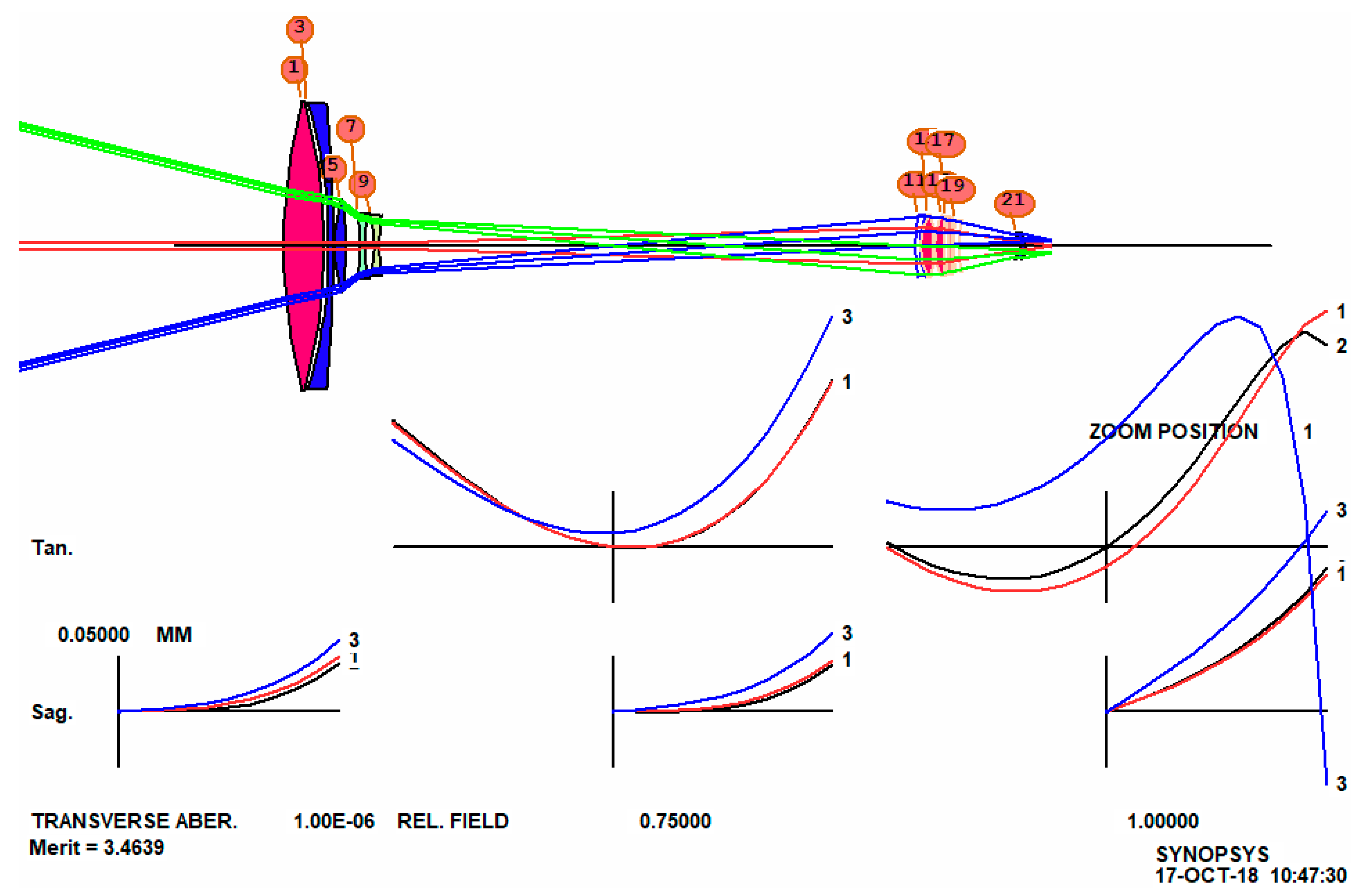
We add the line AEI 7 1 123 0 0 0 50 10 to the optimization MACro and run it again. The lens is further improved, as shown in Figure 12.
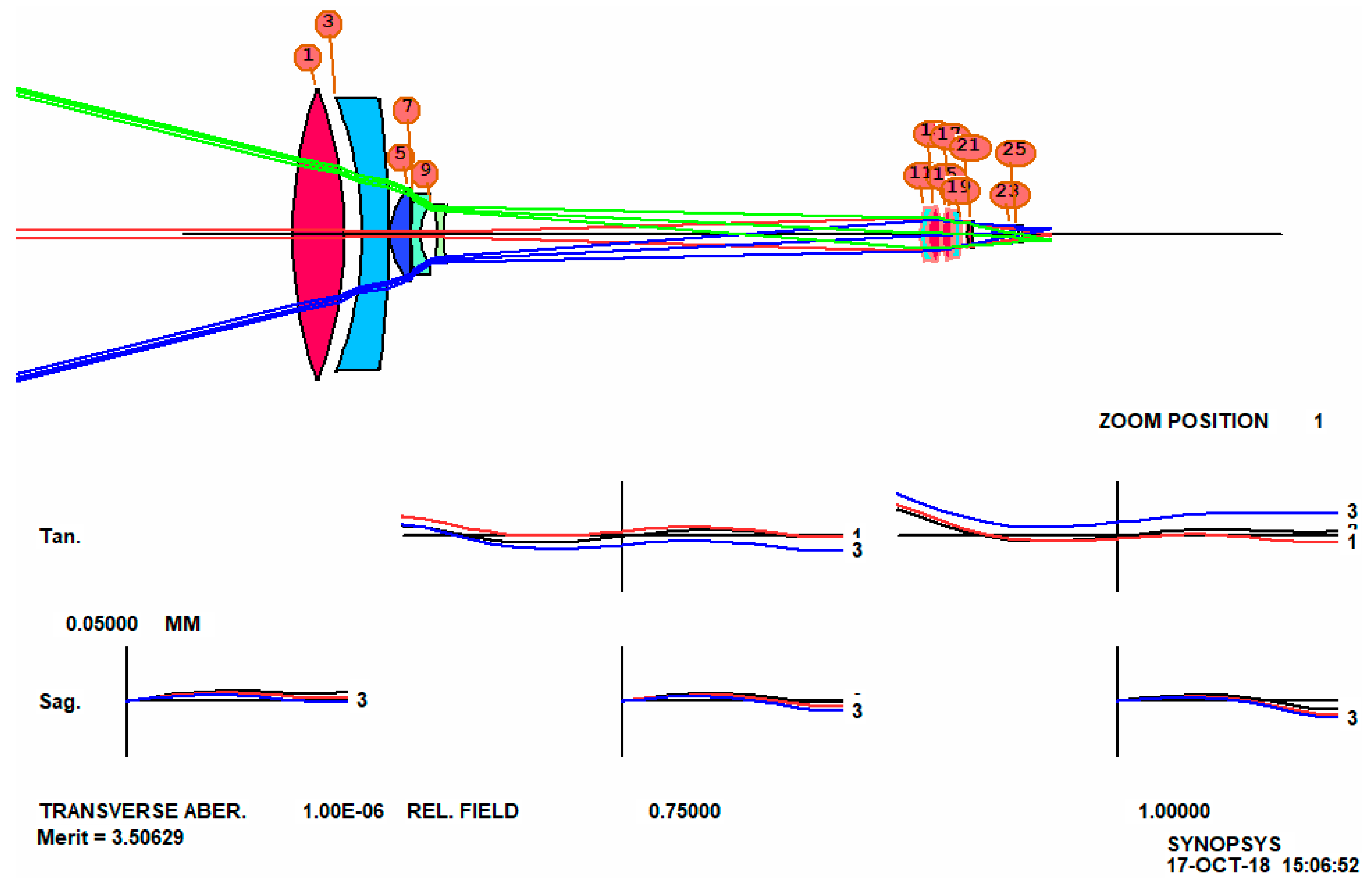
Although numerical methods are powerful, human insight is still important. We note that the largest aberration in the MF is now the requirement to keep lens thicknesses less than one inch, a target added by default by ZSEARCH. But the first element is a large lens, and to correct lateral color it must be allowed to acquire whatever power it needs, and more power means greater thickness. Therefore, we modify the MF, letting the thickness grow. We also add a requirement that the diameter/thickness ratio should be greater than 7.0, which will increase the thickness of those elements that are currently too thin, such as element number 2. Then we run AEI once more, adding one more element. The result is shown in Figure 13. Figure 14 shows the same lens in zoom 15, the long focal length setting. This looks like an excellent design.
Other zoom positions are even better than the extremes shown here. Now we check the performance over the zoom range, using a piecewise cubic interpolation option, and find we have an excellent zoom lens indeed. With these tools, we have in fact been able to go as far as a 90:1 zoom lens, with three moving groups.
It appears that these number crunching tools work very well, and in half a day we have designed a zoom lens that would have required many days or weeks of preliminary layout work using older theoretical methods.
6. Conclusions
We have been surprised how, in many cases, these numerical tools have been able to correct even secondary color, simply by varying the model glass parameters. An older designer once insisted that doing so was impossible without using exotic materials such as calcite. He was wrong, but demonstrating that fact had to wait for the development of these new tools (“Secondary color” refers to the difference in focus between a central wavelength and the longest and shortest. That is historically much harder to control than primary color, which is the difference between just the latter two).
It should be clear that, for these examples, numerical methods (SYNOPSYS, DSEARCH, ZSEARCH, ARGLASS, SPBUILD, and AEI are trademarks of Optical Systems Design, Inc.) vastly outperform the work of expert designers from the last generation. Some of those experts embrace this new technology, while others see it as a threat. I think we should all step back, evaluate the technology carefully, and use its power whenever the problem can be addressed in that way. The younger generation will likely have no qualms about embracing it with enthusiasm.
Funding
This research received no external funding.
Conflicts of Interest
The author declares no conflicts of interest.
Appendix A
The software used in this exercise is SYNOPSYS™ (Optical Systems Design, Inc., East Boothbay, Maine, USA), a product of Optical Systems Design, Inc. Information may be found at www.osdoptics.com.
Appendix B
| CCW | ! CLEAR COMMAND WINDOW |
| CORE 14 | ! AUTHORIZE 14 CORES |
| TIME | ! START A TIMER |
| DSEARCH 1 QUIET | ! RUN DESEARCH |
| SYSTEM | ! BEGIN SYSTEM SPECS |
| ID DSEARCH DG_7 | ! LENS IDENTIFICATION |
| OBA 157.9075 5 17 | ! FINITE OBJECT PARAMETERS |
| WAVL 0.6563 0.5876 0.4861 | ! USE THESE WAVELENGTHS |
| UNITS MM | ! LENS UNITS ARE MM |
| END | ! END OF SYSTEM SECTION |
| GOALS | ! DECLARE DESIGN GOALS |
| ELEMENTS 7 | ! ALLOW 7 ELEMENTS |
| FNUM 4.88 1 | ! TARGET F/NUMBER |
| BACK 157 .01 | ! BACK FOCUS DISTANCE |
| TOTL 80 .01 | ! CELL LENGTH |
| STOP MIDDLE | ! PUT THE STOP IN THE MIDDLE |
| STOP FREE | ! AND LET IT MOVE AROUND |
| RT 0.5 | ! MEDIUM APERTURE WEIGHTING |
| FOV 0.0 0.75 1.0 0.0 0.0 | ! CORRECT AT THREE FIELDS |
| FWT 5.0 3.0 1.0 1.0 1.0 | ! WITH THESE WEIGHTS |
| NPASS 44 | ! 44 OPTIMIZATION CYCLES WHEN DONE |
| ANNEAL 200 20 Q 44 | ! ANNEAL EACH CASE |
| COLORS 3 | ! CORRECT AT THREE COLORS |
| SNAPSHOT 1 | ! MONITOR PROGRESS ON SKETCHPAD DISPLAY |
| TRACK | ! MONITOR PROGRESS |
| QUICK 44 44 | ! USE QUICK METHOD FIRST |
| END | ! END OF GOALS SECTION |
| SPECIAL PANT | ! EXTRA PARAMETERS IF NEEDED |
| END | |
| SPECIAL AANT | ! EXTRA OPERANDS IF NEEDED |
| AEC 1 1 1 | ! AUTO EDGE THICKNESS MONITOR |
| ACC 10 .1 1 | ! AUTO CENTER THICKNESS MONITOR |
| ACM 3 1 1 | ! MINIMUM CENTER THICKNESS MONITOR |
| M -5 1 A GIHT | ! TARGET ON GAUSSIAN IMAGE HEIGHT |
| END | ! END OF DSEARCH INPUT |
| GO | ! RUN DSEARCH |
| TIME | ! SEE HOW LONG THE RUN TOOK |
Appendix C
TIME
CORE 14
DSEARCH 4 QUIET
SYSTEM
ID DSEARCH 3-87
OBB 0 13.5 .04
WAVL 0.6563 0.5876 0.4861
UNITS INCH
END
GOALS
ELEMENTS 6
FNUM 8.32
BACK .631 .01
TOTL .485 .01
STOP MIDDLE
STOP FREE
RT 0.5
FOV 0.0 0.75 1.0 0.0 0.0
FWT 5.0 3.0 1.0 1.0 1.0
NPASS 44
ANNEAL 200 20 Q
COLORS 3
SNAPSHOT 10
TRACK
QUICK 44 44
END
SPECIAL PANT
END
SPECIAL AANT
END
GO
TIME
Appendix D
CORE 14
TIME
DSEARCH 1 QUIET
SYSTEM
ID DSEARCH 7-14
OBB 0 18 0.1
WAVL 0.6563 0.5876 0.4861
UNITS INCH
END
GOALS
ELEMENTS 6
FNUM 5.2
BACK 1.31 .01
TOTL 1.664 .01
STOP MIDDLE
STOP FREE
RT 0.5
FOV 0.0 0.75 1.0 0.0 0.0
FWT 5.0 3.0 1.0 1.0 1.0
NPASS 44
ANNEAL 200 20 Q
COLORS 3
SNAPSHOT 10
QUICK 44 44
END
SPECIAL PANT
END
SPECIAL AANT
ACC .25 1 .1
M 0 1 A P YA 1
S GIHT
END
GO
TIME
Appendix E
SPBUILD 1 QUIET
SYSTEM
ID SPB_7-14
OBB 0 18 0.1
WAVL 0.6563 0.5876 0.4861
UNITS INCH
END
GOALS
ELEMENTS 6
FNUM 5.2
BACK 1.31 0.01
TOTL 1.664 .01
STOP MIDDLE
STOP FREE
RT 0.5
FOV 0.0 0.75 1.0 0.0 0.0
FWT 5.0 3.0 1.0 1.0 1.0
NPASS 44
ANNEAL 200 20 Q
SNAPSHOT 10
TRACK
END
SPECIAL AANT
ACC .1 1 .1
M 0 1 A P YA 1
S GIHT
END
GO
Appendix F
LOG ! to keep track of things later
ON 98
TIME ! to see how long this run took
CORE 14
ZSEARCH 3 QUIET ! save results in library location 3
SYSTEM
ID ZSEARCH TEST
OBB 0 14 3 ! infinite object, 14 degrees semi field, 2.85 mm semi
! aperture. This defines the wide-field object
UNI MM
WAVL CDF
END
GOALS
ZOOMS 7
GROUPS 2 3 4 2 ! lens has four groups with 11 elements altogether
ZGROUP 0 Z Z 0 ! and groups 2 and 3 will zoom
ZFOCUS 5000 4 90 5 ! also correct range focus at 5 meters
FINAL ! declare the desired object at the last zoom position,
! which is the narrow field zoom
OBB 0 0.4666 90
ZSPACE NONLIN 1.7 ! other zoom objects will be nonlinearly spaced between the
! first and last
APS 19 ! put the stop on the first side of the last group
DELAY OFF
GIHT 5 5 10 ! the image height is 5 mm for all zooms, with a weight of 10.
BACK 20 .1 ! the back focus is 20 mm and will vary. A target will be
! added to the merit function with a low weight.
COLOR M ! correct all defined colors
ANNEAL 50 10 Q ! anneal the lens as it is optimized in both modes
QUICK 40 40 ! 40 passes in quick mode, 40 in real-ray mode
ASTART 22
TSTART 12
END
SPECIAL PANT
CUL 1.75
FUL 1.75
END
SPECIAL AANT
ACA 55 1 1 ! monitor rays to keep away from the critical angle.
AEC 2 1 1
ACM 4 1 1
ACC 35 1 1
LUL 600 .1 10 A TOTL
END
GO ! start ZSEARCH
TIME ! see how long the run took.
References
- Kingslake, R.; Johnson, R.B. Lens Design Fundamentals; Academic Press: Bellingham, WA, USA, 2010. [Google Scholar]
- Geary, J.M. Introduction to Lens Design; Willmann-Bell: Richmond, VA, USA, 2011. [Google Scholar]
- Dilworth, D.C. SYNOPSYS Supplement to Joseph M Gary’s Introduction to Lens Design; Willmann-Bell: Richmond, VA, USA, 2013. [Google Scholar]
- Smith, G.H. Practical Computer-Aided Lens Design; Willmann-Bell: Richmond, VA, USA, 2007. [Google Scholar]
- Laiken, M. Lens Design; Marcel Dekker: New York, NY, USA, 1991. [Google Scholar]
- O’Shea, D.C. Elements of Modern Optical Design; Wiley: New York, NY, USA, 1985. [Google Scholar]
- Kingslake, R. Lens Design Fundamentals; Academic Press: New York, NY, USA, 1978. [Google Scholar]
- Dilworth, D.C.; Shafer, D. Man versus machine: A lens design challenge. In Proceedings of the SPIE Optical Engineering + Applications, San Diego, CA, USA, 25 September 2013. [Google Scholar]
- Cox, A. A System of Optical Design; Focal: Waltham, MA, USA, 1964. [Google Scholar]
- Dilworth, D.C. Improved Convergence with the pseudo-second-derivative (PSD) Optimization Method. SPIE 1983, 399, 159–166. [Google Scholar]
- Dilworth, D.C. Automatic Lens Optimization: Recent Improvements. SPIE 1986, 554, 191–196. [Google Scholar]
- Dilworth, D.C. New Tools for the Lens Designer. SPIE 2008, 7060, 70600B. [Google Scholar]
- Berlyn Brixner's Research While Affiliated with Los Alamos National Laboratory and Other Places. Available online: https://www.researchgate.net/scientific-contributions/2039750632_BERLYN_BRIXNER (accessed on 21 November 2018).
- Dilworth, D.C. Lens Design: Automatic and Quasi-Autonomous Computational Methods and Techniques; IOPscience: Bristol, UK, 2018. [Google Scholar]
- Dilworth, D.C. Novel global optimization algorithms: Binary construction and the saddle-point method. In Proceedings of the SPIE Optical Engineering + Applications, San Diego, CA, USA, 11 October 2012. [Google Scholar]
- Saddle Points Reveal Essential Properties of the Merit-function Landscape. Available online: http://spie.org/newsroom/1352-saddle-points-reveal-essential-properties-of-the-merit-function-landscape?SSO=1 (accessed on 24 November 2008).
- Dilworth, D.C. A zoom lens from scratch: The case for number crunching. In Proceedings of the SPIE Optical Engineering + Applications, San Diego, CA, USA, 27 September 2016. [Google Scholar]
Figure 1.
Comparison of convergence rates for several algorithms. Curve A is for PSD III, and curve I is classic damped-least-squares (DLS).
Figure 1.
Comparison of convergence rates for several algorithms. Curve A is for PSD III, and curve I is classic damped-least-squares (DLS).

Figure 2.
Unity-magnification double-Gauss objective, from the literature.

Figure 3.
Results from running DSEARCH on the double-Gauss problem.

Figure 4.
Final design for the double-Gauss problem, with real glass replacing the glass models.

Figure 5.
Design 3-87 from Cox.

Figure 6.
DSEARCH results for the camera lens.

Figure 7.
Design 7-14 from Cox.

Figure 8.
DSEARCH solution to the inverse telephoto lens problem.

Figure 9.
Saddle-point build (SPBUILD) solution to the inverse telephoto problem.

Figure 10.
First results for the 30X zoom lens problem.

Figure 11.
30X zoom optimized with modified targets.

Figure 12.
Zoom lens with element added by automatic element insertion (AEI).

Figure 13.
Zoom lens with thicknesses adjusted by the software, in zoom 1.

Figure 14.
Zoom lens at zoom 15.

© 2018 by the author. Licensee MDPI, Basel, Switzerland. This article is an open access article distributed under the terms and conditions of the Creative Commons Attribution (CC BY) license (http://creativecommons.org/licenses/by/4.0/).
Share and Cite
MDPI and ACS Style
Dilworth, D.C. The Ascendency of Numerical Methods in Lens Design. J. Imaging 2018, 4, 137. https://doi.org/10.3390/jimaging4120137
AMA Style
Dilworth DC. The Ascendency of Numerical Methods in Lens Design. Journal of Imaging. 2018; 4(12):137. https://doi.org/10.3390/jimaging4120137
Chicago/Turabian StyleDilworth, Donald C. 2018. "The Ascendency of Numerical Methods in Lens Design" Journal of Imaging 4, no. 12: 137. https://doi.org/10.3390/jimaging4120137
Note that from the first issue of 2016, this journal uses article numbers instead of page numbers. See further details here.