Analytical Study of Colour Spaces for Plant Pixel Detection

Abstract

Segmentation of regions of interest is an important pre-processing step in many colour image analysis procedures. Similarly, segmentation of plant objects in digital images is an important preprocessing step for effective phenotyping by image analysis. In this paper, we present results of a statistical analysis to establish the respective abilities of different colour space representations to detect plant pixels and separate them from background pixels. Our hypothesis is that the colour space representation for which the separation of the distributions representing object and background pixels is maximized is the best for the detection of plant pixels. The two pixel classes are modelled by Gaussian Mixture Models (GMMs). In our statistical modelling we make no prior assumptions on the number of Gaussians employed. Instead, a constant bandwidth mean-shift filter is used to cluster the data with the number of clusters, and hence the number of Gaussians, being automatically determined. We have analysed the following representative colour spaces: $RGB$, $rgb$, $HSV$, $Ycbcr$ and $CIE$-$Lab$. We have analysed the colour space features from a two-class variance ratio perspective and compared the results of our model with this metric. The dataset for our empirical study consisted of 378 digital images (and their manual segmentations) of a variety of plant species: Arabidopsis, tobacco, wheat, and rye grass, imaged under different lighting conditions, in either indoor or outdoor environments, and with either controlled or uncontrolled backgrounds. We have found that the best segmentation of plants is found using $HSV$ colour space. This is supported by measures of Earth Mover Distance (EMD) of the GMM distributions of plant and background pixels.

1. Introduction

Compared with the growing interest in plant phenotyping using computer vision and image analysis, plant phenotyping by visual inspection is slow and subjective, relying as it does on human evaluation. Two of the aims of digital imaging and image analysis are (a) the removal of any degree of subjectivity associated with an individual human’s perception, and (b) the expedition of the analysis procedure. This is especially important for the high throughput assessment of the phenotypic manifestations of genetic expressions in plants.

Another and particular application of digital imaging in an agricultural setting is the detection and identification of weeds for the purpose of spot spraying of herbicide. Spot spraying, as opposed to blanket spraying, is more economical and environmentally less detrimental. It is worth considering that successful application of spot spraying may also depend on weed size (volume of herbicide) as well as weed identification (type of herbicide). Consequently, being able to estimate weed volume or biomass by 3D reconstruction from digital images is potentially beneficial. In [1], An et al. presented a novel method that used plant segmentation from images for 3D plant morphology quantification and phenotyping. Plant segmentation was used by An et al. in [2] to measure phenotypic traits such as leaf length and rosette area in 2D images. Plant pixel detection by a Gaussian Mixture Model (GMM) was used by Kovalchuk et al. in [3] for the automatic detection of plot canopy coverage and analysis of different genotypes. Thus, it can be noted that an important basic precursor to both detection, identification and 3D reconstruction [4,5] is the process of plant segmentation. That is, the binary classification of pixels into plant and non-plant groups.

There are many approaches to segmentation. These fall into one of two camps: supervised or unsupervised segmentation [4,6]. However, active contours or level sets and fuzzy logic can also be used for object segmentation [7,8]. All these different methods of segmentation will benefit from the study presented in this paper. A colour space which enhances the ability to separate plant pixels from non-plant pixels will improve the performance of any segmentation method based on colour.

Many segmentation methods are based on colour distinction. To achieve optimal plant segmentation, however, the natural question to first pose is which colour space is the more effective for the detection of plant pixels? Is there a suitable transformation of {Red Green Blue} ($RGB$) colour space to a representation that will make plant pixel detection more accurate and more reliable? Can a suitable representation be found that will improve the degree to which plant pixel detection is independent of illumination condition? Does the contrast between plant and background naturally get enhanced in certain colour space irrespective of illumination condition? These are some of the questions we address in this paper. Similar questions have been raised and answered for skin pixel segmentation [9,10,11], shadow and traffic object detection [12,13,14] and image segmentation by graph cut [15,16]. It has been shown in [17] that the choice of colour space does influence object recognition.

A related study seeking to improve plant segmentation by colour analysis was carried out by Golzarian et al. [18] using colour indices. Colour indices, individually however, do not provide a complete representation of a colour space. Individual indices are scalar-valued variables obtained by a linear manipulation of the components of the three dimensional colour space vector of a pixel. The individual colour indices considered by Golzarian et al. [18] were g, $DGR$, $EGI$, $MEGI$, $NDI$, $Hue$, and the hue channel of $HSV$ colour space. Their results showed that hue achieved the least amount of type $II$ error with a small loss of plant pixel. Our results and conclusions differ somewhat. We attribute the difference in conclusions to the fact that our study is more encompassing as our larger dataset includes a greater number of lighting conditions and a larger number of plant species. Thus, in contrast to Golzarian et al.’s findings, our results show that $HSV$ is overall best suited for segmentation of plants under the majority of lighting conditions. An important aspect which has not been addressed in this study is how color balancing would affect the plant pixel detection. Color balancing was shown in [19] to affect texture classification studies.

This paper is organized as follows. In Section 2.1 we introduce briefly the different colour spaces we experimented with and their mathematical relationship to each other. Then, in Section 2.2 we outline our method for discriminating pixels into one of two classes using GMMs and evaluating the separability of the classes by computing their class distance using Earth Mover Distance (EMD) and variance ratios. EMD [20] has a long history for use in image processing and analysis. Rubner et al. used EMD on cluster signature of images for image retrieval and for object tracking by Zhao et al. in [21] and by Kumar et al. in [22]. The details of our dataset are provided in Section 2.3. We present our results and discuss those in Section 3, and finally conclude the paper with summary comments in Section 4.

2. Methods

2.1. Colour Representation

Colour spaces allow for different representations of intensity and colour information in colour images. Past research activities on colour representation, psycho-visual perception of colour, video signal transmission and computer graphics have given rise to many colour spaces having different desirable properties. Here, we briefly review the five well-known colour spaces $RGB$, $rgb$, $HSV$, $Ycbcr$ and $CIE$-$Lab$ that we shall utilize and we summarize how they are related to the common $RGB$ colour space. A consideration of less well-known spaces such as the colour derivative spaces, as described in Gevers et al. [23], and opponent colour space as mentioned in [24] by Gevers and Stokman, could be made the subject of subsequent study.

2.1.1. $RGB$

Red, green and blue are the familiar primary colours and it is now accepted that their different practical combinations are capable of generating almost all possible colour shades. This colour space has been the basis for the design of $CRT$s, television and computer screens. Most still cameras and scanners save their images in this colour space. However, the high correlation between channels as well as the mixing of chrominance and luminance information makes $RGB$ space a sub-optimal choice for colour-based detection schemes.

2.1.2. Normalized $rgb$

$$r=\frac{R}{R+G+B},g=\frac{G}{R+G+B},b=\frac{B}{R+G+B}$$

(1)

This is a colour space in which intensity information is normalized, which in turn leads to a reduced dependence on the luminance information. The normalization property, however, introduces a redundancy amongst the three components. For instance, no additional information is available in b since $b=1-r-g$. In such a case, the components, r and g, are referred to as pure colours due to the absence of a dependence on the brightness of the source $RGB$. A mention of $rg$ space can also be found in [23].

2.1.3. $HSV$

This colour space specifies any colour in terms of three quantities: Hue, Saturation, and Value. It was introduced to satisfy user need to specify colour properties numerically. Hue defines the dominant colour of a pixel, Saturation measures the colourfulness of a pixel in proportion to its brightness, and Value is related to colour luminance. $HSV$ is non-linearly related to $RGB$ via the following set of equations

$$\begin{array}{ccc}\hfill H& =& \left\{\begin{array}{cc}\theta \hfill & \mathit{if}\mathit{B}\le \mathit{G},\hfill \\ 2\pi -\theta \hfill & \mathit{if}\mathit{B}>\mathit{G}.\hfill \end{array}\right.\hfill \\ & & \hfill \mathit{where}\theta =co{s}^{-1}\frac{1/2\left[\right(R-G)+(R-B\left)\right]}{{[{(R-G)}^2+(R-B)(G-B)]}^{1/2}}\\ \hfill S& =& 1-\frac{3}{R+G+B}\left[min(R,G,B)\right]\hfill \\ \hfill V& =& 1/3(R+G+B)\hfill \end{array}$$

(2)

A polar co-ordinate representation of $HSV$ results in a cyclic colour space. $HSV$ colour space was recently used for adaptive skin classification in [25]. This colour space is similar to the colour space representations, $HIS$, $HLS$, and $HCI$.

2.1.4. $Ycbcr$

This colour space is utilized in most image compression standards such as $JPEG$, $H.261$, $MPEG$, and television studios (video cameras also usually save in this format). Pixel intensity is represented by Y luminance, computed as a weighted sum of $RGB$ values; the matrix of weights which transforms the $RGB$ pixel value to $Ycbcr$ is given in Equation (3). The chrominance component of the pixel information is contained in the $cb$ and $cr$ channels. The colour space is characterized by a simple but explicit separation of luminance and chrominance components. It is similar to $YIQ$ and $YUV$ color spaces and linearly related to $RGB$ as follows

$$\left[\begin{array}{c}Y\\ cr\\ cb\end{array}\right]=\left[\begin{array}{ccc}0.299& 0.587& 0.114\\ 0.711& -0.587& -0.114\\ -0.299& -0.587& 0.886\end{array}\right]\times \left[\begin{array}{c}R\\ G\\ B\end{array}\right]$$

(3)

where the matrix elements are fixed.

2.1.5. CIE-Lab

This colour space, originally proposed by G. Wyszecki [26], to approximate perceptually-uniform colour space information has been standardized by the Commission Internationale de L’ Eclairage ($CIE$). By "perceptually-uniform” one means that it was designed to approximate human vision. The L-channel contains information about pixel intensity/brightness, while a and b store the colour information. The $CIE$-$Lab$ colour space is non-linearly related to $CIE$-$XYZ$.

The $RGB$ to $Lab$ conversion is achieved by a transformation , $\mathbf{M}$: $\left[\begin{array}{c}L\\ a\\ b\end{array}\right]=\mathbf{M}\left[\begin{array}{c}R\\ G\\ B\end{array}\right]$. Standard methods exist for specifying the transformation $\mathbf{M}$ when the co-ordinates of the $RGB$ system and reference white has been specified. One such $\mathbf{M}$ has been used in [14] for $sRGB$, $D65$ device-dependent colour space. Related colour spaces are $CIE$-$LUV$ and $CIE$-$LCH$. More details of the different colour spaces could be found in [27].

2.2. Evaluation of Colour Space Representations

To evaluate the suitability of a colour space representation for the detection of plant pixels, we differentiate background from foreground pixels based on their relative position within a GMM which has been constructed using the respective colour space information possessed by the pixels. The Gaussian Mixture Model is a function of a random variable, $\mathbf{z}$, which in our case is the feature vector comprising the information contained in the three pixel colour channels:

$$gmm(\mathbf{z},\mathit{\varphi })=\sum _{k=1}^K{w}_{k}g(\mathbf{z}:{\mathit{\mu }}_k,{\mathbf{\Sigma }}_k)$$

(4)

The model parameter set $\mathit{\varphi }$ is the set ${\{w_k,{\mathit{\mu }}_k,{\mathbf{\Sigma }}_k\}}_{k=1}^K$ where K is the number of Gaussian distributions in $gmm$ and each g is of the form

$$g(\mathbf{z}:{\mathit{\mu }}_k,{\mathbf{\Sigma }}_k)=\frac{1}{\sqrt{2\pi }{\mathbf{\Sigma }}_k}exp\left(-\frac{1}{2}{\left(\frac{\parallel \mathbf{z}-{\mathit{\mu }}_k\parallel }{{\mathbf{\Sigma }}_k}\right)}^2\right).$$

(5)

In applying the GMM using the expectation maximization (EM) algorithm, there arises the fundamental problem of how to predetermine the number of Gaussian functions to include in the GMM. We ameliorate this problem by using a mean-shift algorithm to cluster both the background pixel and foreground plant pixel data. The same fixed bandwidth is used to cluster both sets of pixel data. Each cluster is then modelled as a Gaussian distribution with a diagonal co-variance matrix,

$${\mathbf{\Sigma }}_k=\left[\begin{array}{ccc}{\sigma }_{11}& 0& 0\\ 0& {\sigma }_{22}& 0\\ 0& 0& {\sigma }_{33}\end{array}\right].$$

(6)

This is utilized to reduce computational load at the cost of an insignificant loss of accuracy. We denote the background GMM be $gm{m}_{bg}$ and foreground plant pixel GMM be $gm{m}_{fg}$. A distance function based on Earth Mover Distance (EMD) is used as a measure of the distance between $gm{m}_{bg}$ and $gm{m}_{fg}$. The EMD can be considered as a measure of dissimilarity between two multi-dimensional distributions. The greater the EMD between two distributions the more dissimilar they are. It was used by Rubner et al. in [28] for colour- and texture-based image retrieval. It was also employed by Kumar and Dick in [22] to track targets in an image sequence. In the present case, we apply the EMD measure to the multi-dimensional Gaussian mixture distributions that correspond, respectively, to background and foreground/plant pixel colour in a given colour space. We then consider the relative success of the EMD-based clustering in the different colour spaces to compare the effectiveness of the spaces. The greater the EMD value between the background and foreground GMMs in a given colour space, the better is that colour space for separating plant pixel from non-plant pixel. Using an EMD as a quantifier we aim to discover in which colour space the distance between the two distributions is maximal. We then explore how this distance varies with plant type and imaging condition.

Computing the EMD is based on a solution of the transportation problem [29]. In our case the two distributions are the two GMMs corresponding to the two classes of plant pixel and background pixel:

$$\begin{array}{l}gm{m}_{bg}=\sum _{l=1}^L{w}_{l}g(\mathbf{z}:{\mathit{\mu }}_l,{\mathbf{\Sigma }}_l)and\\ gm{m}_{fg}=\sum _{k=1}^K{w}_{k}g(\mathbf{z}:{\mathit{\mu }}_k,{\mathbf{\Sigma }}_k).\end{array}$$

(7)

Here, $gm{m}_{bg}$ has L Gaussian in its model and $gm{m}_{fg}$ has K. To compute the EMD between them, L need not be equal to K.

2.2.1. EMD on GMMs

In this section we provide an overview of the use of EMD as a measure of separation/distance between two GMM distributions. Let the two distributions, $gm{m}_{bg}$ and $gm{m}_{fg}$, be characterized by their weights, means, and variances, ${(w_l,{\mathit{\mu }}_l,{\mathbf{\Sigma }}_l)}_{l=1}^L$ and ${(w_k,{\mathit{\mu }}_k,{\mathbf{\Sigma }}_k)}_{k=1}^K$. The EMD is used to compute the distance between these cluster signatures. Cluster signatures are characterised by weights; a signature differs from a distribution in the sense that the weights are not normalized. Also, cluster signatures do not have a cluster spread associated with them, since the GMMs have variances associated with each Gaussian. In our case the weights $w_k\{k=1...K\}$ are normalized, i.e., ${\sum }_{k=1}^K{w}_k=1$. EMD can also be used to compute the dissimilarity between unnormalized cluster signatures. However, in our application the weights are normalized. The EMD is defined in terms of an optimal flow $f_{kl}$ which minimizes the following

$$EMD(gm{m}_{fg},gm{m}_{bg})=\sum _{k=1}^K\sum _{l=1}^L{f}_{kl}{d}_{kl},$$

(8)

where $d_{lk}=D(g(\mathbf{z}:{\mathit{\mu }}_k,{\mathbf{\Sigma }}_k),g(\mathbf{z}:{\mathit{\mu }}_l,{\mathbf{\Sigma }}_l))$ is a measure of dissimilarity/distance between Gaussians $g(\mathbf{z}:{\mathit{\mu }}_k,{\mathbf{\Sigma }}_k)$ and $g(\mathbf{z}:{\mathit{\mu }}_l,{\mathbf{\Sigma }}_l)$, and is also referred to as ground distance (GD). The computed flow after an optimization process satisfies the following constraints

$$\begin{array}{ccc}\hfill f_{kl}& \ge & 0,\mathit{for}1\le l\le L,1\le k\le K\hfill \\ \hfill \sum _{l=1}^L{f}_{kl}& \le & w_k,\mathit{for}1\le k\le K\hfill \\ \hfill \sum _{k=1}^K{f}_{kl}& \le & w_l,\mathit{for}1\le l\le L\hfill \\ \sum _{k=1}^K\sum _{l=1}^L{f}_{kl}& =& min(\sum _{k=1}^K{w}_k,\sum _{l=1}^L{w}_l)=1\hfill \end{array}$$

(9)

The formulation of EMD is slightly different when the weights are not normalized. For computing the ground distance $d_{lk}$ we need a distance measure between two Gaussians $g(\mathbf{z}:{\mathit{\mu }}_l,{\mathbf{\Sigma }}_l)$ and $g(\mathbf{z}:{\mathit{\mu }}_k,{\mathbf{\Sigma }}_k)$. We propose here to use a modified Mahalanobis distance to compute the ground distance $d_{lk}$ between Gaussians l and k:

$$d_{lk}={({\mathit{\mu }}_l-{\mathit{\mu }}_k)}^T{[({\mathbf{\Sigma }}_l+{\mathbf{\Sigma }}_k)/2]}^{-1}({\mathit{\mu }}_l-{\mathit{\mu }}_k).$$

(10)

The Mahalanobis distance, formally introduced by P.C. Mahalanobis in [30], is a measure of similarity/difference of a multivariate data point $\mathbf{z}=(z_1,z_2,...,z_N)$ with a known Gaussian distribution in the same dimension

$$D_M\left(\mathbf{z}\right)=\sqrt{{(\mathbf{z}-\mathit{\mu })}^T{\mathbf{\Sigma }}^{-1}(\mathbf{z}-\mathit{\mu })}$$

(11)

This distance is different from Euclidean distance in that it scales down the distance by the standard deviation of the distribution. The intuition behind this distance is that the distance of a data point to a normal distribution is inversely proportional to the latter’s spread. This is an important concept in cluster analysis. The distance of a data point to a cluster is not just the Euclidean distance of the data point to the cluster centre. It also depends inversely on the spread of the cluster. The same intuitive notion extends to the distance between two Gaussians, as suggested by the distance function in Equation (10). The distance between two Gaussians with similar differences in mean values increases as their standard deviation decreases. A problem with the distance function in Equation (10) is that it becomes unbounded as the variance of the Gaussian goes to zero. However, this phenomena is of theoretical interest only, since for real life data sets it is seldom necessary to model something with a zero variance normal distribution. Furthermore, a zero variance normal distribution has no physical meaning. Other distance functions like Bhattacharyya distance, Hellinger distance, Kulback Leibler etc., could also have been modified to formulate a distance function between two multivariate Gaussians and in future studies we will consider this aspect of the problem.

2.2.2. Two-Class Variance Ratio

To study the discriminative power of different colour spaces with respect to segmenting plant pixels from background pixels, we compare the results of the present approach to results of augmented variance ratio (AVR). AVR has been used for feature ranking and as a preprocessing step in feature subset selection [31,32], and for online selection of discriminative feature tracking [33]. AVR is defined as the ratio of the inter-class variance to the intra-class variance of features. We use this variance ratio to measure the power of different colour spaces to discriminate plant pixel from background pixel. It is well known that linear discriminant analysis (LDA) and the variance ratio are inappropriate for separating multi-modal class distributions. The plant pixel colours and background pixel colours are generally multi-model. Therefore, we use the log-likelihood ratio, a non-linear transformation, to transform the features of a pixel i

$$L\left(i\right)=log\frac{max\left(pp\right(i),\delta )}{max\left(bg\right(i),\delta )}$$

(12)

The parameter $\delta$ is set to a small value, e.g., 0.001, to avoid creating a divergence (divide by zero or logarithm of zero). The vectors $pp\left(i\right)$ and $bg\left(i\right)$ are the class-conditional probability distributions (normalized histograms) of plant and background pixels, respectively, learnt from a training data set. This log-likelihood ratio transforms the class distributions into a uni-modal form, making the use of the variance ratio appropriate for measuring the discriminative power of the colour space feature. The variance of $L\left(i\right)$ for class $pp\left(i\right)$ is

$$\begin{array}{lll}var(L;pp)& =& E\left[L^2\left(i\right)\right]-{\left(E\left[L\left(i\right)\right]\right)}^2\\ & =& \sum _{i}pp\left(i\right)L^2\left(i\right)-{\left[\sum _{i}pp\left(i\right)L\left(i\right)\right]}^2\end{array}$$

(13)

Similarly, the variance ratio for the background class is

$$var(L;bg)=\sum _{i}bg\left(i\right)L^2\left(i\right)-{\left[\sum _{i}bg\left(i\right)L\left(i\right)\right]}^2$$

(14)

The variance ratio now is

$$VR(L;pp,bg)=\frac{var(L;(pp+bg)/2)}{var(L;pp)+var(L;bg)}$$

(15)

The denominator ensures that the colour space for which the within-class variance is smaller will be more discriminative, while the numerator favours the feature space in which the between-class variance is larger.

2.3. Dataset and Experiments

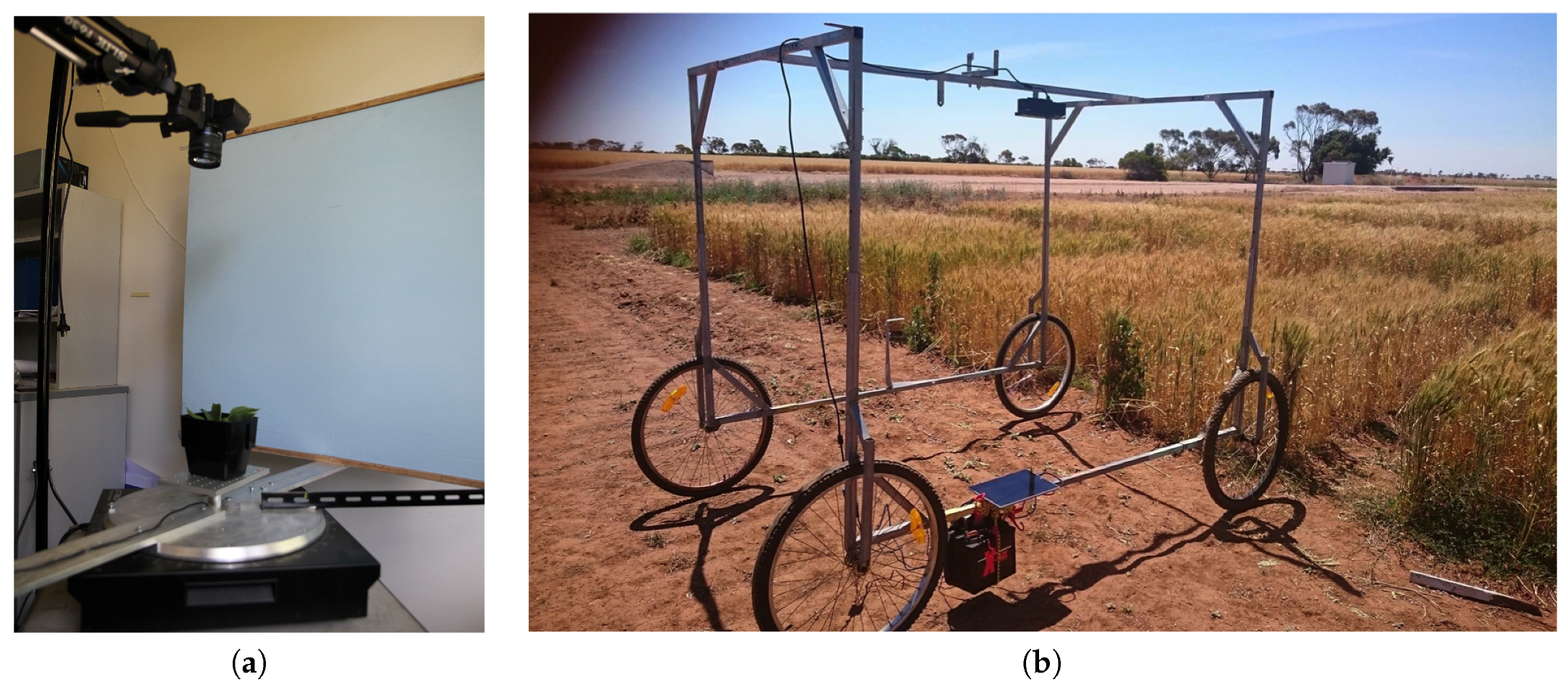
The data set contains images of Arabidopsis and tobacco plants grown in growth chambers which have been taken under controlled lighting conditions. A distinct subset of the data set consists of wheat and rye grass images which have been taken in the field and thus subject to different lighting conditions. Figure 1 shows the two imaging platforms used for imaging some of the plants used in this study. The platform on the left is for imaging indoor plants while the platform on the right is for imaging outdoor plants. After imaging, the plant regions were manually selected and segmented for this study. Arabidopsis images have two types of backgrounds: one black and one red. Plant images were taken both indoors and outdoors in order to capture as great a variety of illumination and background conditions as possible. The complete data set comprises 378 images.

For segmentation of images in different colour spaces we used mean-shift clustering and region fusion. We selected the cluster related to leaves in a semi-supervised way and undertook a two-pass mean-shift clustering. The first pass was to determine the leaf area and separate it from the background. The second pass was to cluster individual leaves and separate them into different leaf areas. Different sets of parameters were used for the two passes of the clustering algorithm as described in [6].

3. Results

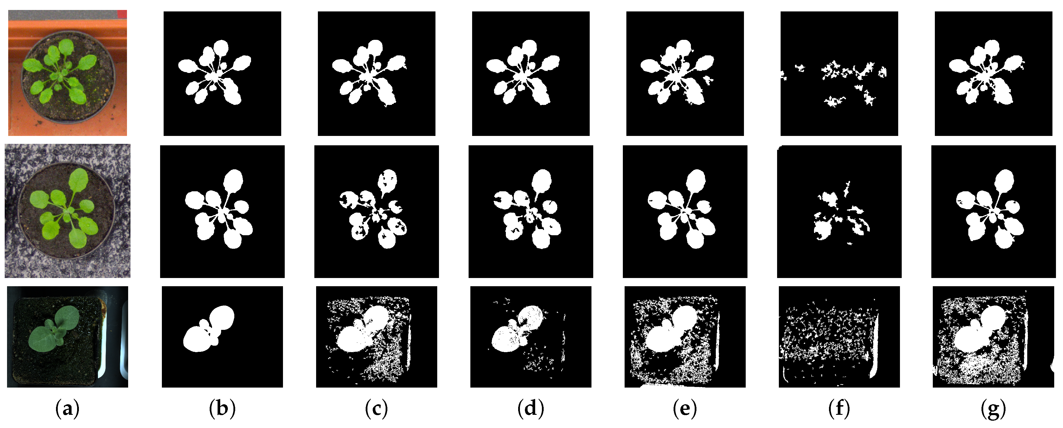
The results of applying the proposed EMD measure, Equation (8), on the GMMs of foreground and background pixels from training data are shown in

Table 1. Table for different plant types and the computed Earth Mover Distance (EMD) on the Gaussian Mixture Models (GMM) models in different colour spaces and their comparison with variance ratio in different colour spaces. EMD based distance are higher for $HSV$ on both plant types, where as variance ratios are higher for normalized $rgb$ colour space.

Plant Type	Colour Space	EMD Distance	Variance Ratio
Arabidopsis	$RGB$	282.46	1.17
	$HSV$	847.24	1.09
	$CIE$-$Lab$	246.14	2.19
	$nrgb$	264.67	2.23
	$YCbCr$	155.01	1.67
Tobacco	$RGB$	228.65	0.76
	$HSV$	1389.56	0.99
	$CIE$-$Lab$	415.17	0.43
	$nrgb$	347.63	1.11
	$YCbCr$	235.15	0.47

and

Table 2. Table for different imaging senarios for same plant type. Their computed EMDs on the GMM models in different colour spaces and their comparsion with variance ratio in different colour spaces. EMD based distance are higher for $HSV$ on both background types, where as variance ratios are higher for normalized $rgb$ colour space for contrasting red background and $CIE$-$Lab$ for the black background.

Background Type	Colour Space	EMD Distance	Variance Ratio
Contrasting Green-Red	$RGB$	230.36	1.07
	$HSV$	401.81	0.78
	$CIE$-$Lab$	182.77	1.77
	$nrgb$	39.43	1.88
	$YCbCr$	178.47	1.57
	$RGB$	282.16	1.27
	$HSV$	404.70	2.13
Green-Black	$CIE$-$Lab$	272.88	9.17
	$nrgb$	257.87	2.24
	$YCbCr$	181.57	3.62

. These tables also show the variance ratios given by Equation (15) for the two classes of pixels in different colour channels. The $HSV$ colour space had the highest scoring of all systems in terms of EMD distance. There appears to be no clear uniformally high performer amongst the different colour spaces, in terms of variance ratio. The segmentation results shown in Figure 2 and in

Table 3. Percentage foreground background segmentation results in the different colour spaces for there different datasets. A1’s are Arabidopsis plants with a red background, A2’s are Arabidopsis plants with black background and A3’s are tobacoo plants imaged in controlled growth chambers.

Plant type	Percentage Foreground Background Segmentation
	$\mathit{RGB}$	$\mathit{HSV}$	$\mathit{CIE}$-$\mathit{Lab}$	$\mathit{rgb}$	$\mathit{YCbCr}$
A1	96.32 %	96.67%	93.40%	10.87%	94.25%
A2	90.53%	98.51%	95.54%	49.69%	97.83%
A3	64.8%	89.6%	57.23%	19.56%	51.79%

show that segmentation based on the HSV colour space was nevertheless superior in two out of three different scenarios. Table 3 shows that segmentation in terms of percentages using the FGBGDice code provided by the LSC challenge dataset. Finally, we show the segmentation results for the test data set in $CIE$-$Lab$ colour space. The reason for using the $CIE$-$Lab$ colour space for this comparison is that this colour space was recommended by the authors of [6].

The segmentation results of separating plant leaves from the background obtained on the test dataset for Arabidopsis images were quite reasonable, achieving mean values of 0.9215 with a standard deviation of 0.0282 on A1 test images (see

Table 4. Overall plant and leaf segmention results using the method of mean-shift clustering as described in Section 2.3.

Plant Type	Plant Segmentation		Leaf Segmentation
	Mean	Std	Mean	Std
A1	92.14%	2.82 %	47.14%	11.14%
A2	93.31%	2.41 %	55.16%	13.15%
A3	76.52%	35.32%	34.03%	22.35%

) and a mean of 0.93313 with a standard deviation of 0.0241 for test images of A2 (see Table 4). Set A1 are Arabidopsis plants with red background imaged indoors under controlled lighting conditions. Set A2 comprised images of Arabidopsis plants with black background also imaged indoors. Set A3 was composed of images of tobacco plants at different stages of development. Some errors in plant and background segmentation were mainly due to the presence of green moss on the background soil. The leaf segmentation results were not as good as the plant segmentation results as the algorithm was designed mainly for background-foreground segmentation. The results can be improved with the use of shape priors for leaf segmentation. The accuracy of plant segmentation for the tobacco test data set was quite poor, which could have resulted for one of two reasons. Firstly, the colours of some of the tobacco plant leaves in the test data set were quite different from what was typically found in the training data set. Secondly, the illumination present in the tobacco images was not as intense as that applied to the Arabidopsis plants. Consequently, some of the darker regions of the tobacco plants have been classified as background.

Plant pixel detection and segmentation is certainly affected by the choice of the colour space being used for image analysis. Hence, the choice of colour space should be given careful consideration for plant phenotyping purposes. In this study where we considered and analysed five different colour spaces, better plant pixel detection was achieved using the $HSV$ colour space for almost all plant types and under different illumination conditions. This can be attributed to the fact that $HSV$ is a perceptual colour space. Usually, best results of detection and segmentation are obtained in perceptual colour spaces. This outcome is supported by Golzarian et al.’s study in [18], where the authors obtained the least amount of type $II$ error with a small loss of plant pixels. However, here we have shown that the segmentation in $HSV$ colour space gives better results under a greater variety of illumination conditions and for a greater range of plant species.

4. Conclusions

In this paper we have presented a method for dynamically selecting the suitability of a feature space (colour space in this case) for segmenting plant pixels in digital images which have both classes of plant pixels and background pixels modelled by Gaussian Mixture Models. For the data set of plants imaged under controlled lighting conditions, the proposed method of colour space selection seems to be more effective than the variance ratio method. The $HSV$ colour space clearly performs better for tobacco plants and is one of the higher quality segmentation performers for Arabidopsis plant images under two different scenarios. This conclusion extends to plants imaged either in field-like conditions where no lighting control is possible, or close to field-like conditions where there is a mix of ambient and controlled lighting. It is well known that the choice colour space influences the performance of image analysis, and the use of perceptual spaces generally provide more satisfying results, whatever database is being considered. Our experimental results on plant pixel detection under different illumination condition supports this prevalent hypothesis. In addition, the separability analysis based on EMD of GMMs for different colour spaces reveals the same phenomena. Our use of different distance functions to measure the separation of Gaussian distributions, and hence $GMMs$, has the added benefit of providing better analytical understanding of the results on which our conclusion is based. In future work we would like to experiment with how color balancing [19] affects the segmentation and detection of plant pixels.

References

- An, N.; Welch, S.M.; Markelz, R.C.; Baker, R.L.; Palmer, C.M.; Ta, J.; Maloof, J.N.; Weinig, C. Quantifying time-series of leaf morphology using 2D and 3D photogrammetry methods for high-throughput plant phenotyping. Comput. Electr. Agric. 2017, 135, 222–232. [Google Scholar] [CrossRef]
- An, N.; Palmer, C.M.; Baker, R.L.; Markelz, R.C.; Ta, J.; Covington, M.F.; Maloof, J.N.; Welch, S.M.; Weinig, C. Plant high-throughput phenotyping using photogrammetry and imaging techniques to measure leaf length and rosette area. Comput. Electr. Agric. 2016, 127, 376–394. [Google Scholar] [CrossRef]
- Kovalchuk, N.; Laga, H.; Cai, J.; Kumar, P.; Parent, B.; Lu, Z.; Miklavcic, S.J.; Haefele, S.M. Phenotyping of plants in competitive but controlled environments: A study of drought response in transgenic wheat. Funct. Plant Biol. 2016, 44, 290–301. [Google Scholar] [CrossRef]
- Kumar, P.; Cai, J.; Miklavcic, S.J. High-throughput 3D modelling of plants for phenotypic analysis. In Proceedings of the 27th Conference on Image and Vision Computing New Zealand; ACM: New York, NY, USA, 2012; pp. 301–306. [Google Scholar]
- Kumar, P.; Connor, J.N.; Miklavcic, S.J. High-throughput 3D reconstruction of plant shoots for phenotyping. In Proceedings of the 2014 13th International Conference on Automation Robotics and Computer Vision (ICARCV), Singapore, 10–12 December 2014. [Google Scholar]
- Comaniciu, D.; Meer, P. Mean Shift: A robust approach toward feature space analysis. IEEE Trans. Pattern Anal. Mach. Intell. 2002, 24, 603–619. [Google Scholar] [CrossRef]
- Golzarian, M.R.; Cai, J.; Frick, R.A.; Miklavcic, S.J. Segmentation of cereal plant images using level set methods, a comparative study. Int. J. Inf. Electr. Eng. 2011, 1, 72–78. [Google Scholar] [CrossRef]
- Valliammal, N.; Geethalakshmi, S.N. A novel approach for plant leaf image segmentation using fuzzy clustering. Int. J. Comput. Appl. 2012, 44, 10–20. [Google Scholar] [CrossRef]
- Phung, S.L.; Bouzerdoum, A.; Chai, D. Skin segmentation using color pixel classification: Analysis and comparison. IEEE Trans. Pattern Anal. Mach. Intell. 2005, 27, 148–154. [Google Scholar] [CrossRef] [PubMed]
- Jones, M.J.; Rehg, J.M. Statistical color models with application to skin detection. J. Comput. Vis. 2002, 46, 81–96. [Google Scholar] [CrossRef]
- Vezhnevets, V.; Sazonov, V.; Andreeva, A. A survey on pixel-based skin color detection techniques. Proc. Graph. 2003, 3, 85–92. [Google Scholar]
- Prati, A.; Mikić, I.; Trivedi, M.M.; Cucchiara, R. Detecting moving shadows: Formulation, algorithms and evaluation. IEEE Trans. Pattern Anal. Mach. Intell. 2003, 25, 918–923. [Google Scholar] [CrossRef]
- Fleyeh, H. Color detection and segmentation for road and traffic signs. Cybern. Intell. Syst. 2004, 2, 809–814. [Google Scholar]
- Kumar, P.; Sengupta, K.; Lee, A. A comparative study of different color spaces for foreground and shadow detection for traffic monitoring system. In Proceedings of the The IEEE 5th International Conference onIntelligent Transportation Systems, Singapore, 6 September 2002; pp. 100–105. [Google Scholar]
- Khattab, D.; Ebied, H.M.; Hussein, A.S.; Tolba, M.F. Color image segmentation based on different color space models using automatic GrabCut. Sci. World J. 2014, 127, 1–10. [Google Scholar] [CrossRef] [PubMed]
- Wang, X.; Hansch, R.; Ma, L.; Hellwich, O. Comparison of different color spaces for image segmentation using Graph-Cut. In Proceedings of the International Conference on Computer Vision Theory and Applications (VISAPP), Lisbon, Portugal, 5–8 January 2014; pp. 301–308. [Google Scholar]
- Muselet, D.; Macaire, L. Combining color and spatial information for object recognition across illumination changes. Pattern Recognit. Lett. 2007, 28, 1176–1185. [Google Scholar] [CrossRef]
- Golzarian, M.R.; Lee, M.K.; Desbiolles, J.M.A. Evaluation of color indices for improved segmentation of plant images. Trans. ASABE 2012, 55, 261–273. [Google Scholar] [CrossRef]
- Bianco, S.; Cusano, C.; Napoletano, P.; Schettini, R. Improving CNN-Based Texture Classification by Color Balancing. J. Imaging 2017, 3, 33. [Google Scholar] [CrossRef]
- Levina, E.; Bickel, P. The earth mover distance is the Mallows distance: Some insights from statistics. In Proceedings of the IEEE International Conference on Computer Vision, Vancouver, BC, Canada, 7–14 July 2001; Volume 2, pp. 251–256. [Google Scholar]
- Zhao, Q.; Brennan, S.; Tao, H. Differential EMD tracking. In Proceedings of the IEEE International Conference on Computer Vision, Rio de Janeiro, Brazil, 14–21 October 2007; pp. 1–8. [Google Scholar]
- Kumar, P.; Dick, A. Adaptive earth mover distance-based Bayesian multi-target tracking. Comput. Vis. IET 2013, 7, 246–257. [Google Scholar] [CrossRef]
- Gevers, T.; Weijer, J.V.D.; Stokman, H. Color Feature Detection: An Overview; Color Image Processing: Methods and Applications; CRC Press: Boca Raton, FL, USA, 2006. [Google Scholar]
- Gevers, T.; Stokman, H. Robust histogram construction from color invariants for object recognition. IEEE Trans. Pattern Anal. Mach. Intell. 2004, 26, 113–118. [Google Scholar] [CrossRef] [PubMed]
- Bianco, S.; Gasparini, F.; Schettini, R. Adaptive Skin Classification Using Face and Body Detection. IEEE Trans. Image Process. 2015, 24, 4756–4765. [Google Scholar] [CrossRef] [PubMed]
- Wyszecki, G.; Stiles, W.S. Color Science: Concepts and Methods, Quantitative Data and Formulae; Wiley: Hoboken, NJ, USA, 2000; Chapter 6. [Google Scholar]
- Busin, L.; Vandenbroucke, N.; Macaire, L. Color spaces and image segmentation. Adv. Imaging Electr. Phys. 2009, 151, 65–168. [Google Scholar]
- Rubner, Y.; Tomasi, C.; Guibas, L.J. The earth mover distance as a metric for image retrieval. Int. J. Comput. Vis. 2000, 40, 99–121. [Google Scholar] [CrossRef]
- Hitchcock, F.L. The distribution of a product from several sources to numerous localities. J. Math. Phys. 1941, 20, 224–230. [Google Scholar] [CrossRef]
- Mahalanobis, P.C. On the generalised distance in statistics. Proc. Natl. Inst. Sci. India 1936, 2, 49–55. [Google Scholar]
- Liu, Y.; Schmidt, K.L.; Cohn, J.F.; Mitra, S. Facial asymmetry quantification for expression invariant human identification. Comput. Vis. Image Underst. 2003, 91, 138–159. [Google Scholar] [CrossRef]
- Liu, Y.; Teverovskiy, L.; Carmichael, O.; Kikinis, R.; Shenton, M.; Carter, C.; Stenger, V.; Davis, S.; Aizenstein, H.; Becker, J.; et al. Discriminative MR image feature analysis for automatic schizophrenia and Alzheimer’s disease classification. In Medical Image Computing and Computer-Assisted Intervention—MICCAI 2004; Barillot, C., Haynor, D., Hellier, P., Eds.; Springer: Berlin/Heidelberg, Germany, 2004; Volume 3216, pp. 393–401. [Google Scholar]
- Collins, R.T.; Liu, Y.; Leordeanu, M. Online selection of discriminative tracking features. IEEE Trans. Pattern Anal. Mach. Intell. 2005, 27, 1631–1643. [Google Scholar] [CrossRef] [PubMed]
Figure 1.
This figure shows the two imaging platforms we have build in house for imaging plants. (a) is the platform for imaging plants indoor and (b) is the platform for imaging outdoor plants growing in field conditions.
Figure 2.
This figure shows the results of segmentation using the method of mean-shift clustering, used in the paper, for different colour spaces. Image in column (a) are the original images of Arabidopsis and Tobacco plants. One set of Arabidopsis plant has a contrasting red background and the other has black background. The images in column (b) are the ground truth segmentation results. The ground truth segmentation were generated by manual labelling of the image data. In columns (c–g) are the segmentation in different colour spaces , , -, normalized , and , respectively.