Edge-Based and Prediction-Based Transformations for Lossless Image Compression


Abstract
:1. Introduction
- (1)
- Providing a framework for ETEC method as a combination of JBE and entropy coding, and then evaluating its effectiveness for compressing a wide range of pixelated images.
- (2)
- Developing a new algorithm termed as PTEC by combining the aspects of hierarchical prediction approach, JBE method, and entropy coding.
- (3)
- Comparing the proposed ETEC and PTEC schemes with the existing compression techniques for a number of pixelated and non-pixelated standard images.
2. Existing Image Compression Techniques
3. Proposed Algorithms
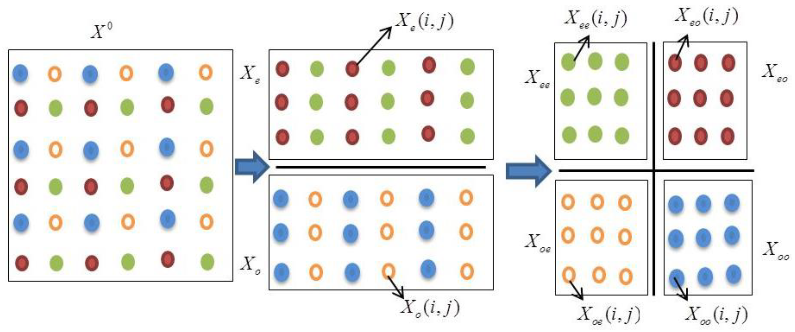
3.1. ETEC
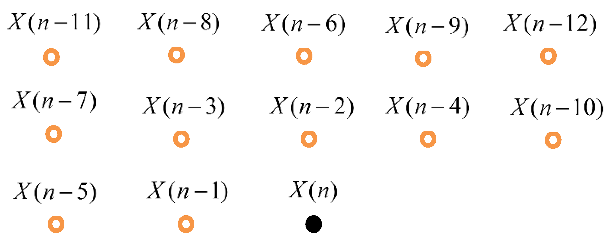
3.2. PTEC
4. Results and Discussion
5. Conclusions
Author Contributions
Funding
Acknowledgments
Conflicts of Interest
References
- Koc, B.; Arnavut, Z.; Kocak, H. Lossless compression of dithered images. IEEE Photonics J. 2013, 5, 6800508. [Google Scholar] [CrossRef]
- Jain, A.K. Image data compression: A review. Proc. IEEE 1981, 69, 349–389. [Google Scholar] [CrossRef]
- Kim, S.; Cho, N.I. Hierarchical prediction and context adaptive coding for lossless color image compression. IEEE Trans. Image Process. 2014, 23, 445–449. [Google Scholar] [CrossRef] [PubMed]
- Kabir, M.A.; Khan, M.A.M.; Islam, M.T.; Hossain, M.L.; Mitul, A.F. Image compression using lifting based wavelet transform coupled with SPIHT algorithm. In Proceedings of the 2nd International Conference on Informatics, Electronics & Vision, Dhaka, Bangladesh, 17–18 May 2013. [Google Scholar]
- Alzahir, S.; Borici, A. An innovative lossless compression method for discrete-color images. IEEE Trans. Image Process. 2015, 24, 44–56. [Google Scholar] [CrossRef] [PubMed]
- Mondal, M.R.H.; Armstrong, J. Analysis of the effect of vignetting on MIMO optical wireless systems using spatial OFDM. J. Lightwave Technol. 2014, 32, 922–929. [Google Scholar] [CrossRef]
- Mondal, M.R.H.; Panta, K. Performance analysis of spatial OFDM for pixelated optical wireless systems. Trans. Emerg. Telecommun. Technol. 2017, 28, e2948. [Google Scholar] [CrossRef]
- Perli, S.D.; Ahmed, N.; Katabi, D. PixNet: Interference-free wireless links using LCD-camera pairs. In Proceedings of the 16th Annual International Conference on Mobile Computing and Networking (MOBICOM), Chicago, IL, USA, 20–24 September 2010. [Google Scholar]
- Shantagiri, P.V.; Saravanan, K.N. Pixel size reduction loss-less image compression algorithm. Int. J. Comput. Sci. Inf. Technol. 2013, 5, 87. [Google Scholar] [CrossRef]
- Ambadekar, S.; Gandhi, K.; Nagaria, J.; Shah, R. Advanced data compression using J-bit Algorithm. Int. J. Sci. Res. 2015, 4, 1366–1368. [Google Scholar]
- Suarjaya, A.D. A new algorithm for data compression optimization. Int. J. Adv. Comput. Sci. Appl. 2012, 3, 14–17. [Google Scholar]
- Al-Azawi, S.; Boussakta, S.; Yakovlev, A. Image compression algorithms using intensity based adaptive quantization coding. Am. J. Eng. Appl. Sci. 2011, 4, 504–512. [Google Scholar]
- Mandyam, G.; Ahmed, N.; Magotra, N. Lossless Image Compression Using the Discrete Cosine Transform. J. Vis. Commun. Image Represent. 1997, 8, 21–26. [Google Scholar] [CrossRef]
- Munteanu, A.; Cornelis, J.; Cristea, P. Wavelet-Based Lossless Compression of Coronary Angiographic Images. IEEE Trans. Med. Imaging 1999, 18, 272–281. [Google Scholar] [CrossRef] [PubMed]
- Taujuddin, N.S.A.M.; Ibrahim, R.; Sari, S. Progressive pixel to pixel evaluation to obtain hard and smooth region for image compression. In Proceedings of the 6th International Conference on Intelligent Systems, Modeling and Simulation, Kuala Lumpur, Malaysia, 9–12 February 2015. [Google Scholar]
- Oh, H.; Bilgin, A.; Marcellin, M.W. Visually Lossless Encoding for JPEG2000. IEEE Trans. Image Process. 2013, 22, 189–201. [Google Scholar] [PubMed]
- Yea, S.; Pearlman, W.A. A Wavelet-Based Two-Stage Near-Lossless Coder. IEEE Trans. Image Process. 2006, 15, 3488–3500. [Google Scholar] [CrossRef] [PubMed]
- Usevitch, B.E. A Tutorial on Modern Lossy Wavelet Image Compression: Foundations of JPEG 2000. IEEE Signal Process. Mag. 2001, 18, 22–35. [Google Scholar] [CrossRef]
- Weinberger, M.J.; Seroussi, G.; Sapiro, G. The LOCO-I Lossless Image Compression Algorithm: Principles and Standardization into JPEG-LS. IEEE Trans. Image Process. 2000, 9, 1309–1324. [Google Scholar] [CrossRef] [PubMed]
- Santos, L.; Lopez, S.; Callico, G.M.; Lopez, J.F.; Sarmiento, R. Performance Evaluation of the H.264/AVC Video Coding Standard for Lossy Hyperspectral Image Compression. IEEE J. Sel. Top. Appl. Earth Obs. Remote Sens. 2012, 5, 451–461. [Google Scholar] [CrossRef]
- Al-Khafaji, G.; Rajab, M.A. Lossless and Lossy Polynomial Image Compression. OSR J. Comput. Eng. 2016, 18, 56–62. [Google Scholar] [CrossRef]
- Wu, X. Lossless Compression of Continuous-Tone Images via Context Selection, Quantization, and Modeling. IEEE Trans. Image Process. 1997, 6, 656–664. [Google Scholar] [PubMed]
- Said, A.; Pearlman, W.A. An Image Multiresolution Representation for Lossless and Lossy Compression. IEEE Trans. Image Process. 1996, 5, 1303–1310. [Google Scholar] [CrossRef] [PubMed]
- Li, X.; Orchard, M.T. Edge-Directed Prediction for Lossless Compression of Natural Images. IEEE Trans. Image Process. 2001, 10, 813–817. [Google Scholar]
- Abo-Zahhad, M.; Gharieb, R.R.; Ahmed, S.M.; Abd-Ellah, M.K. Huffman Image Compression Incorporating DPCM and DWT. J. Signal Inf. Process. 2015, 6, 123–135. [Google Scholar] [CrossRef]
- Lohitha, P.; Ramashri, T. Color Image Compression Using Hierarchical Prediction of Pixels. Int. J. Adv. Comput. Electron. Technol. 2015, 2, 99–102. [Google Scholar]
- Wu, H.; Sun, X.; Yang, J.; Zeng, W.; Wu, F. Lossless Compression of JPEG Coded Photo Collections. IEEE Trans. Image Process. 2016, 25, 2684–2696. [Google Scholar] [CrossRef] [PubMed]
- Kaur, M.; Garg, E.U. Lossless Text Data Compression Algorithm Using Modified Huffman Algorithm. Int. J. Adv. Res. Comput. Sci. Softw. Eng. 2015, 5, 1273–1276. [Google Scholar]
- Rao, D.; Kamath, G.; Arpitha, K.J. Difference based Non-linear Fractal Image Compression. Int. J. Comput. Appl. 2011, 30, 41–44. [Google Scholar]
- Oshri, E.; Shelly, N.; Mitchell, H.B. Interpolative three-level block truncation coding algorithm. Electron. Lett. 1993, 29, 1267–1268. [Google Scholar] [CrossRef]
- Tan, Y.H.; Yeo, C.; Li, Z. Residual DPCM for lossless coding in HEVC. In Proceedings of the 2013 IEEE International Conference on Acoustics, Speech and Signal Processing, Vancouver, BC, Canada, 26–31 May 2013; pp. 2021–2025. [Google Scholar]
- Sanchez, V.; Aulí-Llinàs, F.; Serra-Sagristà, J. DPCM-Based Edge Prediction for Lossless Screen Content Coding in HEVC. IEEE J. Emerg. Sel. Top. Circuits Syst. 2016, 6, 497–507. [Google Scholar] [CrossRef]
- Lainema, J.; Bossen, F.; Han, W.J.; Min, J.; Ugur, K. Intra Coding of the HEVC Standard. IEEE Trans. Circuits Syst. Video Technol. 2012, 22, 1792–1801. [Google Scholar] [CrossRef]
- Sanchez, V.; Aulí-Llinàs, F.; Serra-Sagristà, J. Piecewise Mapping in HEVC Lossless Intra-Prediction Coding. IEEE Trans. Image Process. 2016, 25, 4004–4017. [Google Scholar] [CrossRef] [PubMed]
- Hernández-Cabronero, M.; Marcellin, M.W.; Blanes, I.; Serra-Sagristà, J. Lossless Compression of Color Filter Array Mosaic Images with Visualization via JPEG 2000. IEEE Trans. Multimedia 2018, 20, 257–270. [Google Scholar] [CrossRef]
- Taubman, D.S.; Marcellin, M.W. JPEG2000: Standard for interactive imaging. Proc. IEEE 2002, 90, 1336–1357. [Google Scholar] [CrossRef]
- Egilmez, H.E.; Said, A.; Chao, Y.H.; Ortega, A. Graph-based transforms for inter predicted video coding. In Proceedings of the 2015 IEEE International Conference on Image Processing (ICIP), Quebec City, QC, Canada, 27–30 September 2015; pp. 3992–3996. [Google Scholar]
- Hranilovic, S.; Kschischang, F.R. A pixelated MIMO wireless optical communication system. IEEE J. Sel. Top. Quantum Electron. 2006, 12, 859–874. [Google Scholar] [CrossRef]
- Kabir, M.A.; Mondal, M.R.H. Edge-based Transformation and Entropy Coding for Lossless Image Compression. In Proceedings of the International Conference on Electrical, Computer and Communication Engineering (ECCE), Cox’s Bazar, Bangladesh, 16–18 February 2017; pp. 717–722. [Google Scholar]
- Huffman, D. A method for the construction of minimum redundancy codes. Proc. IRE 1952, 40, 1098–1101. [Google Scholar] [CrossRef]
- Miaou, S.-G.; Chen, S.-T.; Chao, S.-N. Wavelet-based Lossy-to-lossless Medical Image Compression using Dynamic VQ and SPIHT Coding. Biomed. Eng. Appl. Basis Commun. 2003, 15, 235–242. [Google Scholar] [CrossRef]
- Tomar, R.R.S.; Jain, K. Lossless Image Compression Using Differential Pulse Code Modulation and Its Application. Int. J. Signal Process. Image Process. Pattern Recognit. 2016, 9, 197–202. [Google Scholar] [CrossRef]
- Chen, Y.-Y.; Tai, S.-C. Embedded Medical Image Compression using DCT based Subband Decomposition and Modified SPIHT Data Organization. In Proceedings of the IEEE Symposium on Bioinformatics and Bioengineering, Taichung, Taiwan, 21–21 May 2004; pp. 167–175. [Google Scholar]
- Sharma, M. Compression using Huffman Coding. Int. J. Comput. Sci. Netw. Secur. 2010, 10, 133–141. [Google Scholar]
- Salomon, D. A Concise Introduction to Data Compression; Springer: London, UK, 2008. [Google Scholar]
- Wallpaperswide. Available online: http://wallpaperswide.com/pixelate-wallpapers.html (accessed on 23 April 2018).
- Freepik. Available online: https://www.freepik.com/free-photo/pixelated-image_946034.htm (accessed on 23 April 2018).
- Famed Pixelated Paintings. Available online: https://www.trendhunter.com/trends/digitzed-classic-paintings (accessed on 23 April 2018).
- Pixabay. Available online: https://pixabay.com/en/pattern-super-mario-pixel-art-block-1929506/ (accessed on 23 April 2018).
- Image Processing Place. Available online: http://www.imageprocessingplace.com/root_files_V3/image_databases.htm (accessed on 23 April 2018).
- Computational Imaging and Visual Image Processing. Available online: https://www.io.csic.es/PagsPers/JPortilla/image-processing/bls-gsm/63-test-images (accessed on 23 April 2018).
- Wikimedia Commons: Sprgelenkli. Available online: https://commons.wikimedia.org/wiki/File:Sprgelenkli131107.jpg#filelinks (accessed on 23 April 2018).
- Wikimedia Commons: Putamen. Available online: https://commons.wikimedia.org/wiki/File:Putamen.jpg (accessed on 23 April 2018).
- Wikimedia Commons: MRI Glioma 28 Yr Old Male. Available online: https://commons.wikimedia.org/wiki/File:MRI_glioma_28_yr_old_male.JPG (accessed on 23 April 2018).


| Ref. No. | Prediction Based | Wavelet Based | Pixel Difference Based | DCT | Entropy Coding | Image Encoder/Transformer | Image Type | Hierarchical Approach |
|---|---|---|---|---|---|---|---|---|
| [1] | Yes | No | No | No | Yes | PDT | Dithering | No |
| [3] | Yes | No | No | No | Yes | No | Continuous | Yes |
| [5] | No | No | No | No | Yes | Row-column reduction encoding | Map images | No |
| [9] | No | No | No | No | Yes | LZW | Continuous | No |
| [11] | No | No | No | No | Yes | J bit encoding | Continuous | No |
| [12] | No | Yes | No | No | No | AQC | Continuous | No |
| [13] | No | No | Yes | Yes | Yes | No | Continuous | No |
| [14] | No | Yes | No | No | No | Modified EZW | Continuous | No |
| [15] | No | Yes | No | No | No | No | All | No |
| [16] | No | Yes | No | No | No | No | Color | No |
| [17] | No | Yes | No | No | Yes | No | Continuous | No |
| [19] | Yes | No | No | No | Yes | No | Continuous | No |
| [20] | Yes | No | No | No | No | H.264/AVC | Hyper-spectral | No |
| [21] | Yes | No | No | No | Yes | Taylor series | Continuous | No |
| [22] | Yes | No | No | No | Yes | AQC | Continuous | Yes |
| [23] | Yes | No | Yes | No | Yes | S+P transform | Continuous | No |
| [24] | Yes | No | No | No | No | LS based | Natural | No |
| [25] | Yes | Yes | No | No | Yes | No | Medical image | No |
| [26] | Yes | Yes | No | No | No | Color transform | Color | Yes |
| [27] | Yes | No | No | Yes | Yes | Geometric, photometric transformation | JPEG image | No |
| [28] | No | No | No | No | Yes | Dynamic bit reduction | Continuous | No |
| [29] | No | No | Block diff | No | No | No | Fractal | No |
| [30] | No | No | No | No | No | AQC (3-level) | Continuous | No |
| [31] | Yes | No | No | Yes | Yes | residual coding | All | No |
| [32] | Yes | No | No | No | No | residual coding | All | No |
| [33] | Yes | No | No | No | No | residual coding | All | No |
| [34] | Yes | No | No | No | Yes | residual coding | All | No |
| [35] | Yes | Yes | No | No | Yes | residual coding | All | No |
| [36] | Yes | Yes | No | No | Yes | Embedded block coding | All | No |
| [37] | Yes | No | No | No | Yes | Graph based transforms | All | No |
| Tested Image Name | JPEG-LS | Le Gall 5/3 + SPIHT (Subblock) | ETEC (Arithmetic) | PTEC | DPCM | |||||
|---|---|---|---|---|---|---|---|---|---|---|
| Bits/Pixel | CR | Bits/Pixel | CR | Bits/Pixel | CR | Bits/Pixel | CR | Bits/Pixel | CR | |
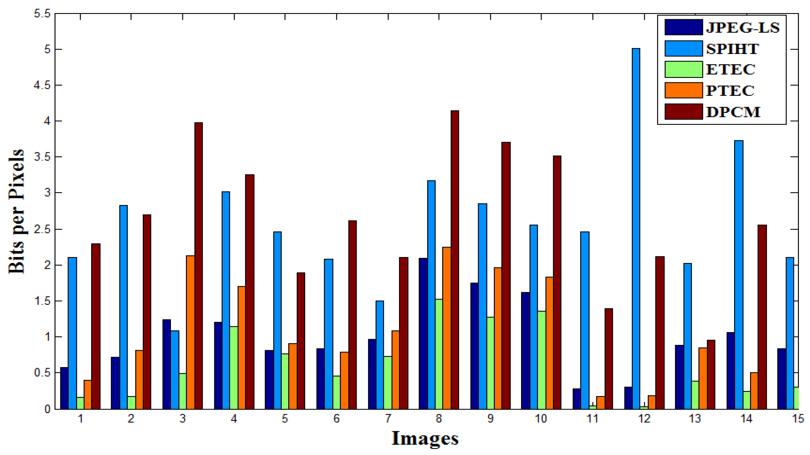
| 1 | 0.573 | 13.95 | 2.105 | 3.8 | 0.162 | 49.52 | 0.393 | 20.35 | 2.29 | 3.49 |
| 2 | 0.715 | 11.19 | 2.822 | 2.84 | 0.176 | 45.42 | 0.812 | 9.85 | 2.70 | 2.96 |
| 3 | 1.236 | 6.47 | 1.084 | 7.38 | 0.493 | 16.23 | 2.128 | 3.76 | 3.98 | 2.01 |
| 4 | 1.202 | 6.65 | 3.021 | 2.65 | 1.145 | 6.98 | 1.702 | 4.70 | 3.25 | 2.46 |
| 5 | 0.814 | 9.83 | 2.465 | 3.25 | 0.764 | 10.48 | 0.905 | 8.84 | 1.89 | 4.22 |
| 6 | 0.834 | 9.59 | 2.085 | 3.84 | 0.457 | 17.52 | 0.783 | 10.22 | 2.61 | 3.06 |
| 7 | 0.964 | 8.3 | 1.495 | 5.35 | 0.734 | 10.9 | 1.08 | 7.41 | 2.10 | 3.81 |
| 8 | 2.098 | 3.81 | 3.172 | 2.52 | 1.527 | 5.24 | 2.241 | 3.57 | 4.14 | 1.93 |
| 9 | 1.744 | 4.58 | 2.846 | 2.81 | 1.271 | 6.29 | 1.956 | 4.09 | 3.70 | 2.16 |
| 10 | 1.618 | 4.94 | 2.555 | 3.13 | 1.36 | 5.88 | 1.831 | 4.37 | 3.52 | 2.27 |
| 11 | 0.282 | 28.4 | 2.462 | 3.25 | 0.046 | 175 | 0.166 | 48.21 | 1.39 | 5.72 |
| 12 | 0.297 | 26.98 | 5.01 | 1.59 | 0.027 | 297 | 0.183 | 43.65 | 2.11 | 3.79 |
| 13 | 0.879 | 9.09 | 2.017 | 3.97 | 0.385 | 20.77 | 0.843 | 9.49 | 0.96 | 8.31 |
| 14 | 1.055 | 7.58 | 3.724 | 2.15 | 0.241 | 33.24 | 0.502 | 15.94 | 2.56 | 3.12 |
| 15 | 0.836 | 9.56 | 2.105 | 3.8 | 0.299 | 26.73 | 0.592 | 13.52 | 2.17 | 3.68 |
| 16 | 1.612 | 4.96 | 2.695 | 2.97 | 1.703 | 4.70 | 1.751 | 4.57 | 2.465 | 3.25 |
| 17 | 2.279 | 3.51 | 4.662 | 1.72 | 2.396 | 3.34 | 2.312 | 3.46 | 3.714 | 2.15 |
| 18 | 2.265 | 3.53 | 3.295 | 2.43 | 2.209 | 3.62 | 2.281 | 3.51 | 4.020 | 1.99 |
| 19 | 1.723 | 4.64 | 2.536 | 3.15 | 1.509 | 5.30 | 1.699 | 4.71 | 3.173 | 2.52 |
| 20 | 2.838 | 2.82 | 3.669 | 2.18 | 2.422 | 3.30 | 2.689 | 2.98 | 4.348 | 1.84 |
| 21 | 0.713 | 11.23 | 2.172 | 3.68 | 0.713 | 11.23 | 1.117 | 7.16 | 3.030 | 2.64 |
| 22 | 0.094 | 85.47 | 1.623 | 4.93 | 0.094 | 85.47 | 0.305 | 26.24 | 1.774 | 4.51 |
| 23 | 0.778 | 10.28 | 2.462 | 3.25 | 0.254 | 31.51 | 0.783 | 10.22 | 3.237 | 2.47 |
| 24 | 1.588 | 5.04 | 3.827 | 2.09 | 1.865 | 4.29 | 1.599 | 5.00 | 3.030 | 2.64 |
| 25 | 1.539 | 5.20 | 2.963 | 2.70 | 1.594 | 5.02 | 1.597 | 5.01 | 1.770 | 4.52 |
| 26 | 1.398 | 5.72 | 2.669 | 3.00 | 0.948 | 8.44 | 1.377 | 5.81 | 2.180 | 3.67 |
| 27 | 1.590 | 5.03 | 3.499 | 2.29 | 1.608 | 4.98 | 1.594 | 5.02 | 1.932 | 4.14 |
| 28 | 0.683 | 11.72 | 2.492 | 3.21 | 0.087 | 92.28 | 0.914 | 8.75 | 1.946 | 4.11 |
| 29 | 1.750 | 4.57 | 2.724 | 2.94 | 1.264 | 6.33 | 1.729 | 4.63 | 3.721 | 2.15 |
| 30 | 1.678 | 4.77 | 2.617 | 3.06 | 1.376 | 5.81 | 1.633 | 4.90 | 3.540 | 2.26 |
| 31 | 1.468 | 5.45 | 2.006 | 3.99 | 1.931 | 4.14 | 1.882 | 4.25 | 4.494 | 1.78 |
| 32 | 2.900 | 2.76 | 3.724 | 2.15 | 3.067 | 2.61 | 3.030 | 2.64 | 4.571 | 1.75 |
| 33 | 0.422 | 18.95 | 1.868 | 4.28 | 0.025 | 326.28 | 0.086 | 92.55 | 1.460 | 5.48 |
| 34 | 1.257 | 6.36 | 2.346 | 3.41 | 0.766 | 10.45 | 1.192 | 6.71 | 2.606 | 3.07 |
| 35 | 0.876 | 9.14 | 2.075 | 3.86 | 0.803 | 9.96 | 0.872 | 9.17 | 1.843 | 4.34 |
| 36 | 1.198 | 6.68 | 2.271 | 3.52 | 1.118 | 7.16 | 1.236 | 6.47 | 2.410 | 3.32 |
| 37 | 1.586 | 5.04 | 2.759 | 2.90 | 1.630 | 4.91 | 1.590 | 5.03 | 3.053 | 2.62 |
| 38 | 1.714 | 4.67 | 2.756 | 2.90 | 3.101 | 2.58 | 2.920 | 2.74 | 4.908 | 1.63 |
| 39 | 1.965 | 4.07 | 2.985 | 2.68 | 1.889 | 4.23 | 1.961 | 4.08 | 4.020 | 1.99 |
| 40 | 1.701 | 4.70 | 3.105 | 2.58 | 1.727 | 4.63 | 1.766 | 4.53 | 3.478 | 2.30 |
| 41 | 0.990 | 8.08 | 2.466 | 3.24 | 0.847 | 9.44 | 0.986 | 8.11 | 2.540 | 3.15 |
| 42 | 1.510 | 5.30 | 2.630 | 3.04 | 1.180 | 6.78 | 1.594 | 5.02 | 3.376 | 2.37 |
| 43 | 1.078 | 7.42 | 2.525 | 3.17 | 0.742 | 10.79 | 1.077 | 7.43 | 2.508 | 3.19 |
| 44 | 1.135 | 7.05 | 2.522 | 3.17 | 0.832 | 9.62 | 1.105 | 7.24 | 2.581 | 3.10 |
| 45 | 0.988 | 8.09 | 2.298 | 3.48 | 0.608 | 13.16 | 0.974 | 8.21 | 2.410 | 3.32 |
| 46 | 0.944 | 8.48 | 2.321 | 3.45 | 0.601 | 13.31 | 0.905 | 8.84 | 2.332 | 3.43 |
| 47 | 1.560 | 5.13 | 3.189 | 2.51 | 1.242 | 6.44 | 1.610 | 4.97 | 3.463 | 2.31 |
| 48 | 1.428 | 5.60 | 2.889 | 2.77 | 1.141 | 7.01 | 1.518 | 5.27 | 3.125 | 2.56 |
| 49 | 1.792 | 4.46 | 3.197 | 2.50 | 1.924 | 4.16 | 1.900 | 4.21 | 3.419 | 2.34 |
| 50 | 1.261 | 6.34 | 2.362 | 3.39 | 0.903 | 8.86 | 1.252 | 6.39 | 2.888 | 2.77 |
| Average | 0.836 | 9.264 | 2.105 | 3.178 | 0.299 | 29.39 | 0.592 | 10.28 | 2.17 | 3.09 |
| Tested Image No. | JPEG-LS | Le Gall 5/3 + SPIHT (Subblock) | ETEC (Arithmetic) | PTEC | DPCM | |||||
|---|---|---|---|---|---|---|---|---|---|---|
| Saving % | Time (s) | Saving % | Time (s) | Saving % | Time (s) | Saving % | Time (s) | Saving % | Time (s) | |
| 1 | 92.83 | 295 | 73.68 | 20.8 | 97.98 | 134.5 | 95.09 | 22.93 | 71.33 | 31.5 |
| 2 | 91.06 | 309 | 64.79 | 16.7 | 97.8 | 133.65 | 89.85 | 28.35 | 66.23 | 35.05 |
| 3 | 84.54 | 495 | 86.45 | 38.5 | 93.84 | 126.74 | 73.40 | 49.21 | 50.24 | 48.23 |
| 4 | 84.96 | 751 | 62.26 | 18.72 | 85.69 | 92.12 | 78.72 | 30.42 | 59.39 | 29.26 |
| 5 | 89.83 | 389 | 69.23 | 17.52 | 90.46 | 78.63 | 88.69 | 20.82 | 76.32 | 19.64 |
| 6 | 89.57 | 501 | 73.96 | 14.94 | 94.29 | 74.13 | 90.22 | 19.31 | 67.32 | 25.25 |
| 7 | 87.95 | 405 | 81.31 | 7.25 | 90.83 | 43.01 | 86.50 | 17.92 | 73.76 | 17.44 |
| 8 | 73.75 | 235 | 60.32 | 3.55 | 80.91 | 3.76 | 71.99 | 9.9 | 48.18 | 9.34 |
| 9 | 78.2 | 246 | 64.41 | 3.61 | 84.12 | 3.66 | 75.55 | 7.02 | 53.81 | 8.66 |
| 10 | 79.76 | 247 | 68.05 | 3.40 | 83.00 | 3.57 | 77.12 | 8.23 | 56.00 | 7.95 |
| 11 | 96.48 | 114 | 69.23 | 2.34 | 99.43 | 16.18 | 97.93 | 5.53 | 82.51 | 9.17 |
| 12 | 96.29 | 92 | 37.3 | 7.44 | 99.66 | 16.03 | 97.71 | 5.57 | 73.63 | 12.75 |
| 13 | 89.01 | 840 | 74.81 | 24.84 | 95.19 | 164.5 | 89.46 | 15.01 | 87.97 | 7.26 |
| 14 | 86.82 | 862 | 53.49 | 34.5 | 96.99 | 221.58 | 93.73 | 44.17 | 67.95 | 38.56 |
| 15 | 91.47 | 407 | 68.85 | 21.22 | 98.92 | 93.44 | 92.60 | 3.14 | 72.84 | 45.29 |
| 16 | 79.84 | 788 | 66.31 | 18.71 | 78.71 | 98.08 | 78.12 | 20.82 | 69.19 | 15.67 |
| 17 | 71.51 | 779 | 41.72 | 25.15 | 70.05 | 102.80 | 71.10 | 35.04 | 53.57 | 28.52 |
| 18 | 71.69 | 180 | 58.81 | 2.49 | 72.39 | 2.77 | 71.49 | 4.8 | 49.75 | 4.23 |
| 19 | 78.47 | 196 | 68.29 | 2.76 | 81.14 | 2.70 | 78.77 | 5.09 | 60.33 | 4.35 |
| 20 | 64.53 | 277 | 54.14 | 3.79 | 69.73 | 4.68 | 66.39 | 5.61 | 82.17 | 3.60 |
| 21 | 85.23 | 149 | 72.85 | 2.17 | 86.03 | 1.26 | 86.03 | 3.89 | 62.12 | 2.78 |
| 22 | 94.85 | 625 | 79.71 | 25.72 | 98.83 | 255.55 | 96.19 | 39.48 | 77.83 | 33.47 |
| 23 | 90.27 | 360 | 69.22 | 11.10 | 96.83 | 31.93 | 90.21 | 12.72 | 59.54 | 9.52 |
| 24 | 80.16 | 370 | 52.16 | 11.24 | 76.68 | 23.60 | 80.02 | 5.57 | 62.12 | 3.75 |
| 25 | 82.52 | 833 | 66.63 | 18.71 | 88.15 | 95.19 | 82.79 | 25.75 | 72.75 | 22.43 |
| 26 | 80.76 | 1130 | 62.96 | 24.16 | 80.08 | 137.40 | 80.04 | 38.19 | 77.88 | 31.36 |
| 27 | 80.12 | 1152 | 56.27 | 27.60 | 79.90 | 142.31 | 80.08 | 39.71 | 75.85 | 35.09 |
| 28 | 91.46 | 407 | 68.85 | 21.22 | 98.92 | 93.44 | 88.57 | 27.05 | 75.67 | 23.68 |
| 29 | 78.13 | 234 | 65.96 | 3.21 | 84.20 | 3.40 | 78.39 | 5.47 | 53.49 | 3.39 |
| 30 | 81.64 | 291 | 74.92 | 4.89 | 75.86 | 4.64 | 76.47 | 7.52 | 43.82 | 23.5 |
| 31 | 63.75 | 326 | 53.45 | 3.86 | 61.66 | 8.09 | 62.12 | 6.85 | 42.86 | 31.52 |
| 32 | 79.02 | 173 | 67.29 | 2.43 | 82.80 | 2.41 | 79.59 | 4.09 | 55.75 | 6.15 |
| 33 | 94.72 | 118 | 76.65 | 6.98 | 99.69 | 16.48 | 98.92 | 11.32 | 81.75 | 5.43 |
| 34 | 84.28 | 1600 | 70.68 | 35.25 | 90.43 | 27.98 | 85.10 | 43.52 | 67.43 | 11.27 |
| 35 | 89.05 | 784 | 74.07 | 22.64 | 89.96 | 121.54 | 89.09 | 29.46 | 76.96 | 18.32 |
| 36 | 85.03 | 170 | 71.61 | 3.32 | 86.03 | 3.34 | 84.54 | 5.09 | 69.88 | 3.05 |
| 37 | 80.18 | 118 | 65.51 | 1.92 | 79.63 | 2.18 | 80.12 | 3.71 | 61.83 | 2.54 |
| 38 | 78.57 | 174 | 65.55 | 1.78 | 61.24 | 2.66 | 63.50 | 3.15 | 38.65 | 2.71 |
| 39 | 75.44 | 567 | 62.69 | 6.93 | 76.38 | 14.65 | 75.49 | 9.37 | 49.75 | 8.52 |
| 40 | 78.74 | 723 | 61.19 | 10.65 | 78.41 | 22.53 | 77.92 | 15.80 | 56.52 | 12.63 |
| 41 | 87.62 | 390 | 69.18 | 9.91 | 89.41 | 21.68 | 87.67 | 15.24 | 68.25 | 13.04 |
| 42 | 81.13 | 275 | 67.13 | 3.63 | 85.25 | 4.00 | 80.08 | 5.40 | 57.81 | 3.96 |
| 43 | 86.53 | 966 | 68.43 | 23.45 | 90.73 | 65.22 | 86.54 | 29.43 | 68.65 | 23.79 |
| 44 | 85.81 | 914 | 68.47 | 24.47 | 89.60 | 121.80 | 86.19 | 32.26 | 67.74 | 25.64 |
| 45 | 87.65 | 922 | 71.28 | 22.10 | 92.40 | 131.33 | 87.82 | 32.04 | 69.88 | 25.54 |
| 46 | 88.21 | 859 | 70.99 | 22.34 | 92.49 | 133.39 | 88.69 | 31.47 | 70.85 | 24.98 |
| 47 | 80.50 | 602 | 60.14 | 9.10 | 84.47 | 18.17 | 79.88 | 13.85 | 56.71 | 11.07 |
| 48 | 82.15 | 673 | 63.89 | 11.30 | 85.73 | 24.07 | 81.02 | 18.90 | 60.94 | 14.00 |
| 49 | 77.60 | 1254 | 60.03 | 20.83 | 75.95 | 119.82 | 76.25 | 27.27 | 57.26 | 21.77 |
| 50 | 84.24 | 717 | 70.47 | 13.68 | 88.71 | 62.66 | 84.35 | 17.86 | 63.90 | 14.45 |
| Average | 83.48 | 526 | 66.11 | 13.90 | 86.15 | 62.58 | 82.76 | 18.406 | 64.54 | 17.42 |
| Tested Image No. | JPEG-LS | Le Gall 5/3 + SPIHT (Subblock) | ETEC (Arithmetic) | PTEC | DPCM | |||||
|---|---|---|---|---|---|---|---|---|---|---|
| Bits/Pixel | CR | Bits/Pixel | CR | Bits/Pixel | CR | Bits/Pixel | CR | Bits/Pixel | CR | |
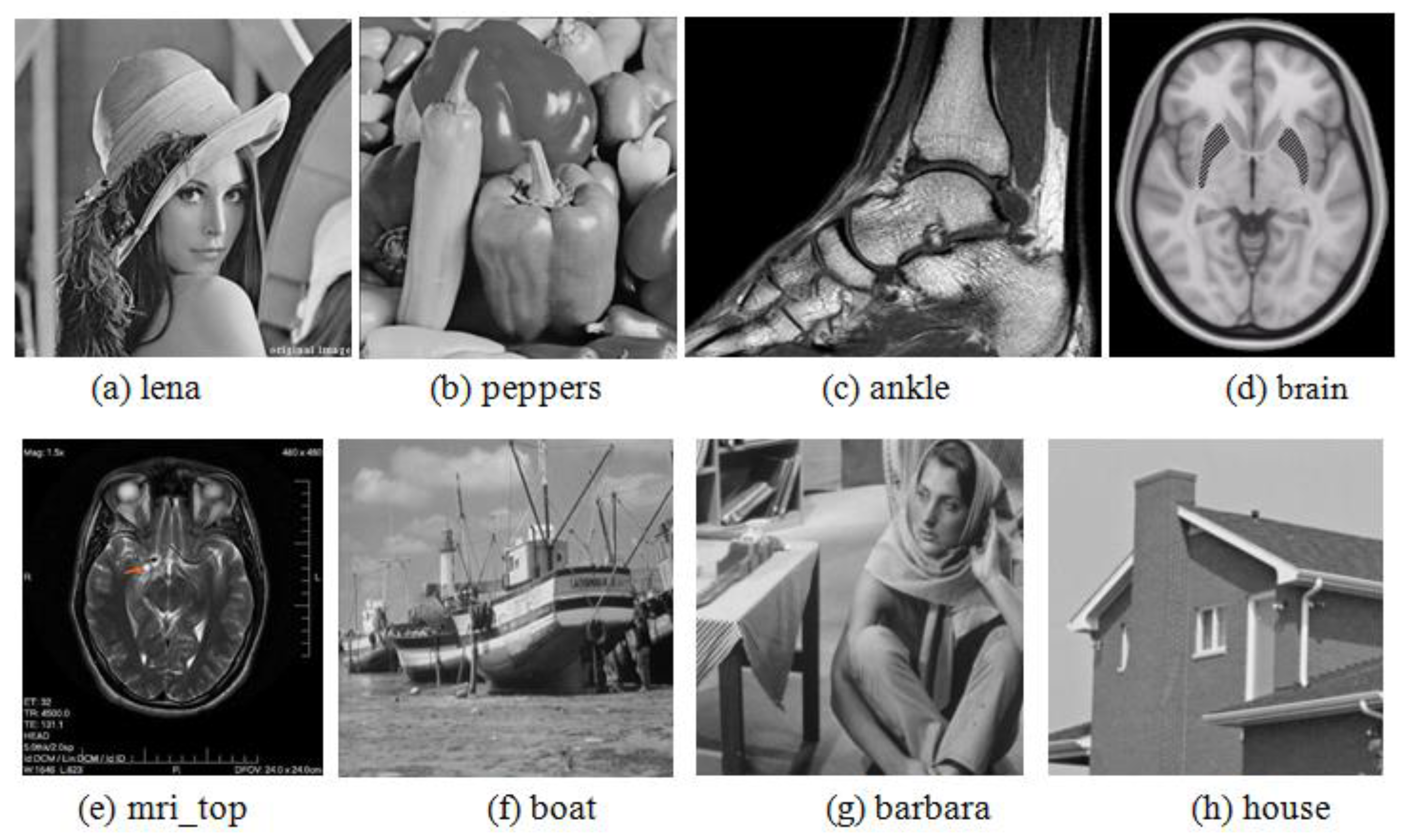
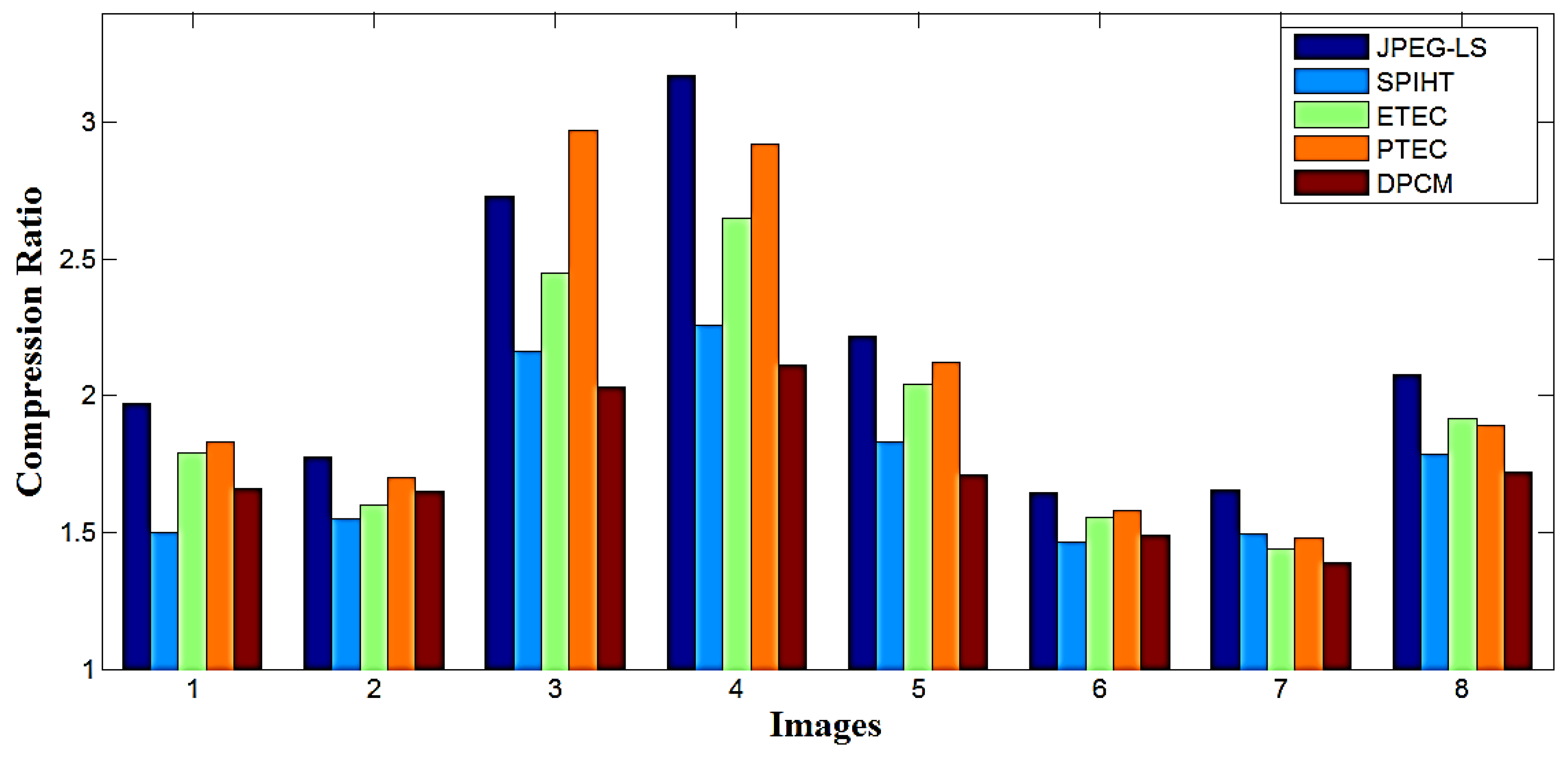
| lena | 4.0567 | 1.972 | 5.3404 | 1.498 | 4.464 | 1.792 | 4.364 | 1.83 | 4.81 | 1.66 |
| peppers | 4.5050 | 1.775 | 5.1543 | 1.552 | 4.998 | 1.601 | 4.704 | 1.70 | 4.84 | 1.65 |
| ankle | 2.93 | 2.73 | 3.704 | 2.16 | 3.265 | 2.45 | 2.694 | 2.97 | 3.940 | 2.03 |
| brain | 2.52 | 3.17 | 3.54 | 2.26 | 3.019 | 2.65 | 2.74 | 2.92 | 3.791 | 2.11 |
| mri_top | 3.60 | 2.22 | 4.372 | 1.83 | 3.922 | 2.04 | 3.774 | 2.12 | 4.678 | 1.71 |
| boat | 4.8618 | 1.645 | 5.4581 | 1.465 | 5.15 | 1.553 | 5.067 | 1.58 | 5.35 | 1.49 |
| barbara | 4.8280 | 1.657 | 5.3452 | 1.496 | 5.559 | 1.439 | 5.402 | 1.48 | 5.74 | 1.39 |
| house | 3.8535 | 2.076 | 4.4817 | 1.785 | 4.176 | 1.915 | 4.227 | 1.89 | 4.64 | 1.72 |
| Average | 3.89 | 2.16 | 4.67 | 1.76 | 4.32 | 1.93 | 4.12 | 2.06 | 4.72 | 1.72 |
| Tested Image No. | JPEG-LS | Le Gall 5/3 + SPIHT (Subblock) | ETEC (Arithmetic) | PTEC | DPCM | |||||
|---|---|---|---|---|---|---|---|---|---|---|
| Saving % | Time (s) | Saving % | Time (s) | Saving % | Time (s) | Saving % | Time (s) | Saving % | Time (s) | |
| lena | 49.29 | 2934 | 33.24 | 59.7 | 44.2 | 330.26 | 45.451 | 97.16 | 39.92 | 53.70 |
| peppers | 43.69 | 1705 | 35.57 | 76.27 | 37.527 | 390.89 | 41.197 | 104.6 | 39.52 | 54.87 |
| ankle | 63.37 | 1548.7 | 53.70 | 22.13 | 59.18 | 398.25 | 66.33 | 37.63 | 50.74 | 27.29 |
| brain | 68.45 | 1761.67 | 55.75 | 36.62 | 62.26 | 500.39 | 65.75 | 61.43 | 52.61 | 29.94 |
| mri_top | 54.95 | 1941.48 | 45.36 | 34.25 | 50.98 | 393.27 | 52.83 | 62.12 | 41.52 | 33.76 |
| boat | 39.23 | 3352 | 31.77 | 58.19 | 35.625 | 397 | 36.665 | 106.3 | 33.03 | 60.86 |
| barbara | 39.65 | 4037 | 33.18 | 50.70 | 30.517 | 355.47 | 32.473 | 109.1 | 28.22 | 72.41 |
| house | 51.83 | 955 | 43.98 | 9.7 | 47.794 | 14.13 | 47.163 | 17.6 | 41.96 | 15.01 |
| Average | 51.30 | 2279.36 | 41.57 | 43.45 | 46.01 | 347.44 | 48.48 | 74.50 | 40.85 | 43.48 |
© 2018 by the authors. Licensee MDPI, Basel, Switzerland. This article is an open access article distributed under the terms and conditions of the Creative Commons Attribution (CC BY) license (http://creativecommons.org/licenses/by/4.0/).
Share and Cite
Kabir, M.A.; Mondal, M.R.H. Edge-Based and Prediction-Based Transformations for Lossless Image Compression. J. Imaging 2018, 4, 64. https://doi.org/10.3390/jimaging4050064
Kabir MA, Mondal MRH. Edge-Based and Prediction-Based Transformations for Lossless Image Compression. Journal of Imaging. 2018; 4(5):64. https://doi.org/10.3390/jimaging4050064
Chicago/Turabian StyleKabir, Md. Ahasan, and M. Rubaiyat Hossain Mondal. 2018. "Edge-Based and Prediction-Based Transformations for Lossless Image Compression" Journal of Imaging 4, no. 5: 64. https://doi.org/10.3390/jimaging4050064