LaBGen-P-Semantic: A First Step for Leveraging Semantic Segmentation in Background Generation

Abstract

Given a video sequence acquired from a fixed camera, the stationary background generation problem consists of generating a unique image estimating the stationary background of the sequence. During the IEEE Scene Background Modeling Contest (SBMC) organized in 2016, we presented the LaBGen-P method. In short, this method relies on a motion detection algorithm for selecting, for each pixel location, a given amount of pixel intensities that are most likely static by keeping the ones with the smallest quantities of motion. These quantities are estimated by aggregating the motion scores returned by the motion detection algorithm in the spatial neighborhood of the pixel. After this selection process, the background image is then generated by blending the selected intensities with a median filter. In our previous works, we showed that using a temporally-memoryless motion detection, detecting motion between two frames without relying on additional temporal information, leads our method to achieve the best performance. In this work, we go one step further by developing LaBGen-P-Semantic, a variant of LaBGen-P, the motion detection step of which is built on the current frame only by using semantic segmentation. For this purpose, two intra-frame motion detection algorithms, detecting motion from a unique frame, are presented and compared. Our experiments, carried out on the Scene Background Initialization (SBI) and SceneBackgroundModeling.NET (SBMnet) datasets, show that leveraging semantic segmentation improves the robustness against intermittent motions, background motions and very short video sequences, which are among the main challenges in the background generation field. Moreover, our results confirm that using an intra-frame motion detection is an appropriate choice for our method and paves the way for more techniques based on semantic segmentation.

1. Introduction

Given a video sequence acquired from a fixed camera, the stationary background generation problem (also known as background initialization, background estimation, background extraction or background reconstruction) consists of generating a unique image estimating the stationary background of the sequence (i.e., the set of objects that are motionless from beginning to end). The generation of a background image is helpful for many computer vision tasks including video surveillance, segmentation, compression, inpainting, privacy protection and computational photography [1].

Estimating the stationary background of a given video sequence is challenging in real-world conditions. For instance, a simple method such as the pixel-wise temporal median filter fails at generating a clean background image when the background is occluded by foreground objects more than half of the time. To tackle the different difficulties occurring in complex scenes (e.g., intermittent motions, camera jitter, illumination changes, shadows, etc.), more sophisticated methods have emerged over the years (see [1,2,3] for some comprehensive surveys on this topic). Among these methods, we have presented LaBGen [4,5], which was ranked number one during the Scene Background Modeling and Initialization (SBMI) workshop in 2015 (http://sbmi2015.na.icar.cnr.it) and the IEEE Scene Background Modeling Contest (SBMC) in 2016 (http://pione.dinf.usherbrooke.ca/sbmc2016); and LaBGen-P [6], an improvement to LaBGen (http://www.telecom.ulg.ac.be/labgen). To summarize the principles in short, LaBGen-P relies on a motion detection algorithm for selecting, for each pixel location, a given amount of pixel intensities that are most likely static by keeping the ones with the smallest quantities of motion. The quantities of motion are estimated by aggregating the motion scores returned by the motion detection algorithm in the spatial neighborhood of the pixel. After this selection process, the background image is then generated by blending the selected intensities with a median filter.

In a previous work, we have shown experimentally that, using a temporally-memoryless motion detection, detecting motion between two frames without relying on additional temporal information (e.g., by using the frame difference, or an optical flow) enables our background generation methods to achieve the best average performance [7]. In addition, we led an experiment suggesting that, as long as we increase the amount of temporal memory used by a simple motion detector, the average performance of our methods decreases. This observation motivates us to deepen the question of temporally-memoryless motion detections for background generation.

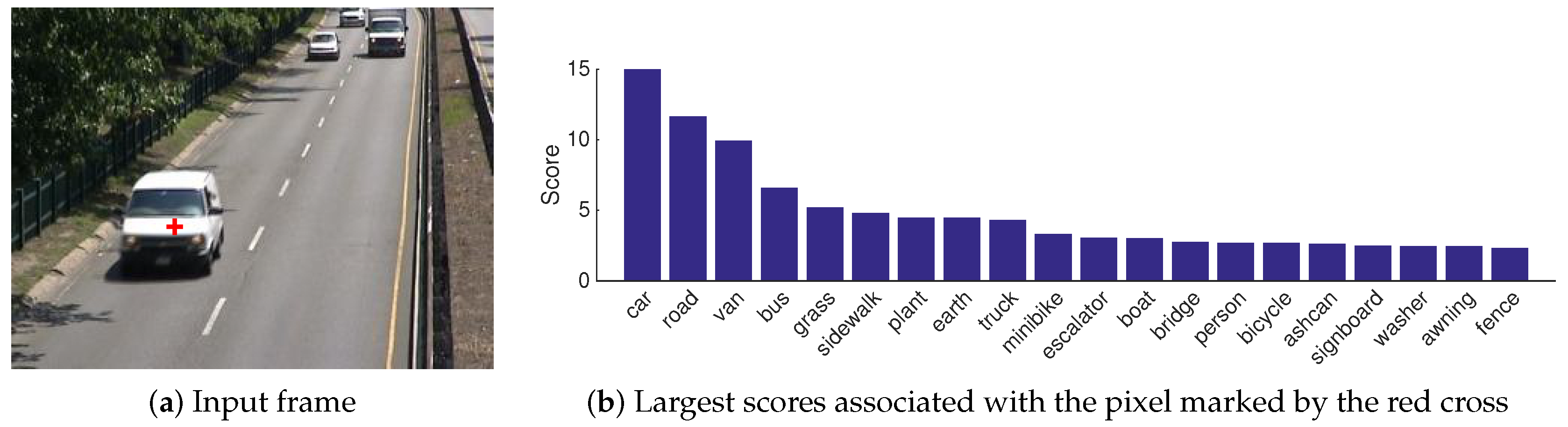
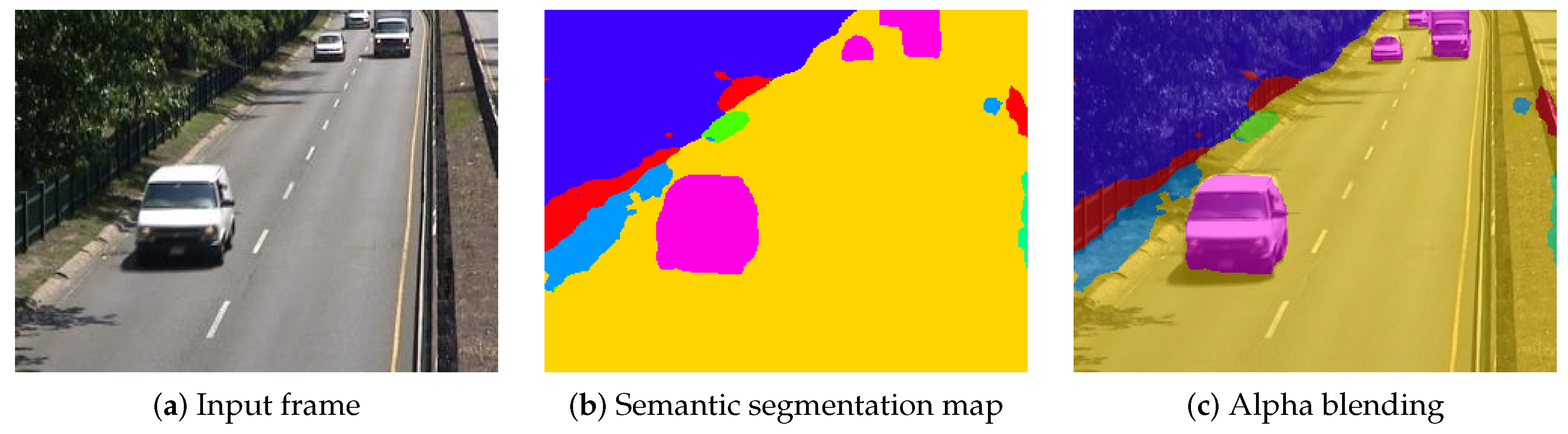
In 2017, Braham et al. introduced a new paradigm for motion detection combining a background subtraction algorithm to an intra-frame motion detection algorithm built on the current frame only by using semantic segmentation [8]. A semantic segmentation algorithm (also known as object segmentation, scene parsing and scene labeling) is trained to recognize a restricted set of objects from spatial features and returns a vector of scores for each pixel of a given frame. In such a vector, each score is associated with a specific object class and quantifies the membership to this class (see Figure 1). When the vector of scores is replaced by the name of the object class with the largest score, one obtains semantic segmentation maps, indicating for each pixel the object depicted by its intensity (see Figure 2). To perform an intra-frame motion detection, after mapping the vector of scores to a vector of probabilities, Braham et al. suggest to aggregate the resulting probabilities by summing the ones associated with object classes that one considers as belonging to the foreground.

With the rise of deep learning in recent years, semantic segmentation algorithms have reached impressive accuracies on complex datasets (see http://sceneparsing.csail.mit.edu). Furthermore, by relying on spatial features only, we believe that using semantic segmentation for background generation can improve, in addition to the global performance, the robustness against intermittent motion misdetections, which is one of the main challenges in the field [3]. Therefore, in this paper, we describe how to leverage semantic segmentation for background generation in a variant of LaBGen-P, called LaBGen-P-Semantic. For this purpose, we replace the mechanism of aggregation of probabilities of Braham et al. by incorporating it in a Bayesian framework and propose two different intra-frame motion detection algorithms built upon semantic segmentation and based on different hypotheses.

The paper is organized as follows. Section 2 details the principles of LaBGen-P. Section 3 presents our two new intra-frame motion detection algorithms leveraging semantic segmentation and how they are included in LaBGen-P-Semantic. Section 4 describes our experiments and discusses our results. Finally, Section 5 concludes this paper.

2. The LaBGen-P Stationary Background Generation Method

Given an input video sequence composed of $T>1$ frames $F^1,F^2,\dots ,F^T$, with a width $w>0$ and a height $h>0$, LaBGen-P [6] generates an image of size $w\times h$, estimating the stationary background $B$ of this sequence. LaBGen-P, which is an improvement of the original LaBGen method [4,5], is comprised of four steps. First, the motion detection step computes, for each pixel, a motion score by leveraging a motion detection algorithm (see Section 2.1). Then, the estimation step refines the result of the previous one by computing quantities of motion combining the motion scores spatially (see Section 2.2). Once the estimation step is done, the selection step builds, for each pixel location, a subset of a given amount of pixel intensities whose pixels are associated with the smallest quantities of motion (see Section 2.3). Finally, the generation step produces the background image by combining the pixel intensities selected in the different subsets built during the selection step. This combination is performed by applying a median filter on the pixel intensities selected in the subsets (see Section 2.4). Thus, unlike a traditional median filter combining all pixel intensities encountered over time, LaBGen-P combines only the ones that most likely belong to the background. The four steps of LaBGen-P are detailed hereafter.

2.1. Step 1: Motion Detection Step

In order to get quantities of motion, it is necessary to detect motion first. For this purpose, we challenged the contribution of several background subtraction algorithms with LaBGen [5], the method on which LaBGen-P is based. For a given frame $F^t$, with $t=2,3,\dots ,T$, they provide a segmentation map indicating which pixels belong to the foreground by using a classification process based on the comparison between a background model and the frame $F^t$. The background model can be based either on statistics [10], subspace learning [11], robust decomposition into low-rank plus sparse matrices [12], or tensors [13], or fuzzy models [14] (see [15] for a comprehensive review on background subtraction). Note that the first frame is skipped as no motion information can be extracted from a unique frame when (spatio-)temporal features are used. According to our previous experiments [5], the frame difference algorithm provides the most adequate motion detection, and it outperforms other, more complex, background subtraction algorithms. Therefore, we decided to use this algorithm in LaBGen-P. For a given pixel, it returns a motion score by computing the absolute difference of pixel intensities between the current and previous frames. Let $p_{x,y}^t$, with $x=0,1,\dots ,w-1$ and $y=0,1,\dots ,h-1$, the pixel at position $\left(x,y\right)$ in frame $F^t$; $I_{x,y}^t$ the intensity of this pixel; and $m_{x,y}^t$ the motion score associated with this pixel, it follows that:

$$m_{x,y}^t=\left|I_{x,y}^t-I_{x,y}^{t-1}\right|.$$

(1)

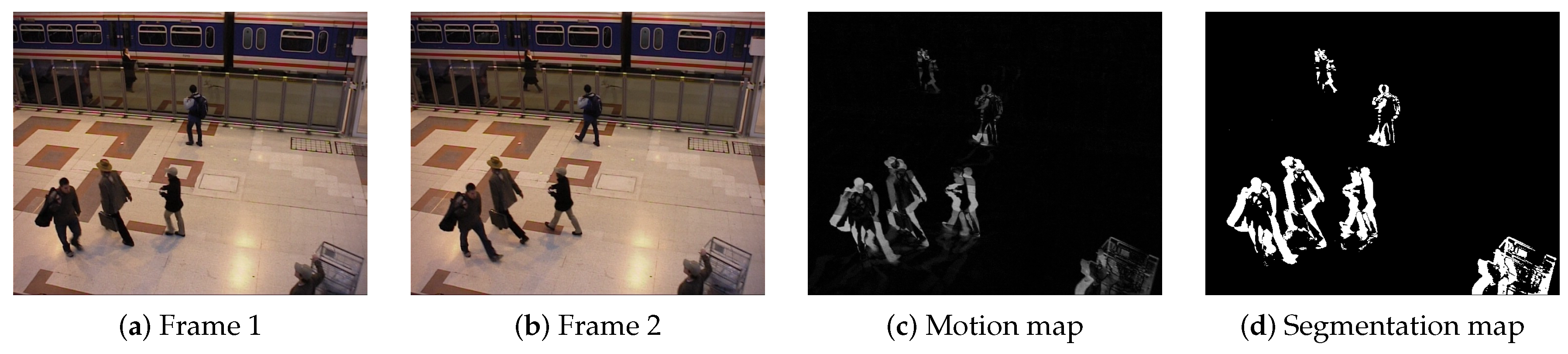
To get a binary classification indicating whether the pixel $p_{x,y}^t$ belongs to the foreground in frame $F^t$, a hard threshold must be applied on the motion score $m_{x,y}^t$. Instead of leveraging segmentation maps, we leverage motion maps in LaBGen-P. A motion map $m_{}^t$ provides the motion scores associated with the pixels in a frame $F^t$. Working with motion maps avoids the need to find a correct hard threshold and enables the method to capture some shades about observed motions. The difference between a segmentation map and a motion map is illustrated in Figure 3.

2.2. Step 2: Estimation Step

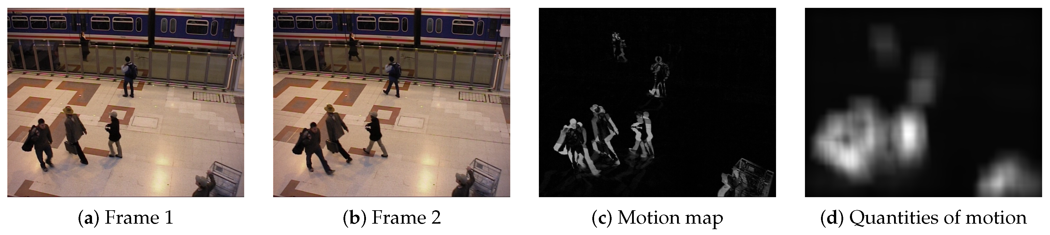
Instead of relying only on temporal information for motion detection, LaBGen-P refines the motion scores computed during the previous step by estimating a quantity of motion $q_{x,y}^t$ for each pixel $p_{x,y}^t$ in frame $F^t$, with $t=2,3,\dots ,T$. Specifically, a quantity of motion $q_{x,y}^t$ is estimated spatially by aggregating the motion scores available in the local neighborhood of pixel $p_{x,y}^t$. The need for such an estimation can be illustrated with a simple example. With an algorithm such as the frame difference, the inside of a moving object is detected as stationary, unlike its edges (this phenomenon can be observed in the motion map of Figure 3). Thus, if quantities of motion were equivalent to motion scores (if $q_{x,y}^t=m_{x,y}^t)$, the pixels within a moving object should be considered as background candidates since their quantities of motion would be near or equal to zero. To avoid such a behavior, a quantity of motion $q_{x,y}^t$ is estimated as follows.

Let ${\mathsf{\Psi }}_{x,y}$ be a set of pixel positions inside a rectangular window around $\left(x,y\right)$. Given a frame $F^t$, the quantity of motion $q_{x,y}^t$ associated with the pixel $p_{x,y}^t$ aggregates the motion scores of the pixels whose positions are included in the set ${\mathsf{\Psi }}_{x,y}$ by summing them:

$$q_{x,y}^t=\sum _{\left(x^{\prime },y^{\prime }\right)\in {\mathsf{\Psi }}_{x,y}}{m}_{x^{\prime },y^{\prime }}^t.$$

(2)

The size of the rectangular window is determined by an odd value W, which is a function of the dimensions w and h of the input video sequence, and a parameter $\mathcal{N}\in {\mathbb{N}}^{*}$. More precisely, the parameter $\mathcal{N}$ divides the minimum dimension of the input video sequence such that:

$$W=1+2⌊\frac{min\left(w,h\right)}{2\mathcal{N}}⌋.$$

(3)

Note that $\mathcal{N}=\infty$ is a special case in which the estimation step is ignored and, thus, where a quantity of motion $q_{x,y}^t$ is equal to the motion score $m_{x,y}^t$.

When a square window of dimensions $W\times W$ can be centered on pixel position $\left(x,y\right)$ without exceeding the borders of the image plane, the positions inside this window are included into the set ${\mathsf{\Psi }}_{x,y}$. On the contrary, the boundaries of the window are modified to consider only the positions that are not outside the limits of the image plane. Thus, the set ${\mathsf{\Psi }}_{x,y}$ is defined as follows:

$${\mathsf{\Psi }}_{x,y}=\left\{\left(x^{\prime },y^{\prime }\right)\left|\begin{array}{cc}{x}^{\prime }\le min\left(x+⌊W/2⌋,w-1\right)\hfill & \bigwedge \\ x^{\prime }\ge max\left(x-⌊W/2⌋,0\right)\hfill & \bigwedge \\ y^{\prime }\le min\left(y+⌊W/2⌋,h-1\right)\hfill & \bigwedge \\ y^{\prime }\ge max\left(y-⌊W/2⌋,0\right)\hfill \end{array}\right.\right\}.$$

(4)

The difference between motion scores and quantities of motion is illustrated in Figure 4.

Finally, it should be noted that, when implemented, the computation of the quantities of motion can be sped up by using summed area tables [16]. After an initialization phase whose complexity is $\mathcal{O}\left(wh\right)$, a summed area table enables one to compute any quantity of motion in a constant time $\mathcal{O}\left(1\right)$, regardless of the position and size of the window being used.

2.3. Step 3: Selection Step

Once the quantities of motion are computed, the purpose of the selection step is to filter out the pixel intensities depicting moving objects over time. In other words, LaBGen-P builds, for each pixel position $\left(x,y\right)$, a subset ${\mathsf{\Omega }}_{x,y}^{}$ of maximum $\mathcal{S}\in {\mathbb{N}}^{*}$ intensities among the set of candidates $\left\{I_{x,y}^2,I_{x,y}^3,\dots ,I_{x,y}^T\right\}$, according to the quantities of motion $q_{x,y}^2,q_{x,y}^3,\dots ,q_{x,y}^T$.

The selection step builds the subset ${\mathsf{\Omega }}_{x,y}^{}$ iteratively. The subset of pixel intensities selected after processing the frame $F^t$ is referred to as ${\mathsf{\Omega }}_{x,y}^t$. When the cardinality of the subset ${\mathsf{\Omega }}_{x,y}^{t-1}$ is less than the parameter $\mathcal{S}$, the pixel intensity $I_{x,y}^t$ is automatically added into ${\mathsf{\Omega }}_{x,y}^t$. Otherwise, $I_{x,y}^t$ is added into ${\mathsf{\Omega }}_{x,y}^t$ when the quantity of motion $q_{x,y}^t$ is less than at least one quantity of motion associated with a pixel whose intensity is selected in ${\mathsf{\Omega }}_{x,y}^{t-1}$. In this case, to keep the cardinality of ${\mathsf{\Omega }}_{x,y}^t$ equal to the parameter $\mathcal{S}$, the pixel intensity $I_{x,y}^{\beta }$ selected in ${\mathsf{\Omega }}_{x,y}^{t-1}$, and whose pixel is associated with the largest quantity of motion $q_{x,y}^{\beta }$, is removed from ${\mathsf{\Omega }}_{x,y}^t$. With such a rule, the intensities whose pixels are considered in motion are iteratively replaced with ones whose pixels are considered as belonging to the background of the input video sequence. Note that if two or more intensities selected in ${\mathsf{\Omega }}_{x,y}^{t-1}$ are associated with pixels sharing the quantity of motion $q_{x,y}^{\beta }$, the oldest selection is discarded. The selection step is summarized in the following equation:

$${\mathsf{\Omega }}_{x,y}^t=\left\{\begin{array}{cc}\varnothing \hfill & \mathrm{for}t=1,\hfill \\ {\mathsf{\Omega }}_{x,y}^{t-1}\cup \left\{I_{x,y}^t\right\}\hfill & \mathrm{for}t=2,3,\dots ,\mathcal{S}+1,\hfill \\ {\mathsf{\Omega }}_{x,y}^{t-1}\cup \left\{I_{x,y}^t\right\}\setminus \left\{I_{x,y}^{\beta }\right\}\hfill & \mathrm{if}t>\mathcal{S}+1\bigwedge q_{x,y}^t\le q_{x,y}^{\beta },\hfill \\ {\mathsf{\Omega }}_{x,y}^{t-1}\hfill & \mathrm{otherwise}.\hfill \end{array}\right.$$

(5)

After processing the last frame $F^T$, the selection step is completed. Consequently, the final subset of pixel intensities ${\mathsf{\Omega }}_{x,y}^{}$ corresponding to pixel position $\left(x,y\right)$ is defined as follows:

$${\mathsf{\Omega }}_{x,y}^{}={\mathsf{\Omega }}_{x,y}^T.$$

(6)

2.4. Step 4: Generation Step

After the selection step, the final step aims at generating the background image returned by LaBGen-P. Its principle is to combine, for each pixel position, the intensities selected in the corresponding subset of pixel intensities using a channel-wise median filter. Depending on the application, a first estimate of the background image might be required as soon as possible. Thus, the generation step can be run either in an online or offline mode, whose principles are the following:

• Online mode: A background image $B_{}^t$ is generated after the processing of each frame $F^t$, starting from the second one. Consequently, the channel-wise median filter is applied on each intermediate subset of intensities ${\mathsf{\Omega }}_{x,y}^t$. Thus, the background intensity $B_{x,y}^t$ corresponding to pixel position $\left(x,y\right)$ after the processing of frame $F^t$ is generated as follows:

  $$B_{x,y}^t=median\left({\mathsf{\Omega }}_{x,y}^t\right).$$

  (7)
• Offline mode: A unique background image $B_{}^{}=B_{}^T$ is generated after processing the final frame $F^T$. The background intensity $B_{x,y}^{}$ corresponding to pixel position $\left(x,y\right)$ is generated as follows:

  $$B_{x,y}^{}=median\left({\mathsf{\Omega }}_{x,y}^{}\right).$$

  (8)
  Even though only the subset of intensities ${\mathsf{\Omega }}_{x,y}^{}$ is used in this mode, building all intermediate subsets ${\mathsf{\Omega }}_{x,y}^t$, with $t=2,3,\dots ,T-1$, in the estimation step is necessary to build ${\mathsf{\Omega }}_{x,y}^{}$ iteratively. Note that using the offline mode offers a better computational performance as the generation step is applied only after a unique frame. In return, one has to wait for the end of the processing of the whole input video sequence to get a background estimate.

3. LaBGen-P-Semantic: The First Background Generation Method Leveraging Semantics

Hereafter, we present LaBGen-P-Semantic, a variant of LaBGen-P (see Section 2) leveraging semantic segmentation in the motion detection step. We consider a semantic segmentation algorithm trained to recognize N distinct object classes $\left[1\right],\left[2\right],\dots ,\left[N\right]$, and returning a N-dimensional vector of scores ${\mathbf{s}}_{x,y}^t=\left[s_{x,y}^t\left(1\right),s_{x,y}^t\left(2\right),\dots ,s_{x,y}^t\left(N\right)\right]$ for a given pixel $p_{x,y}^t$. Specifically, a value $s_{x,y}^t\left(i\right)\in \mathbb{R}$, for each $i=1,2,\dots ,N$, provides the score that the object depicted in $p_{x,y}^t$ is $0_i$. The problem with relying on such an algorithm for detecting motion is to figure out how to get a unique motion score $m_{x,y}^t$ from the vector of scores ${\mathbf{s}}_{x,y}^t$. First, it is common to map the vector of scores ${\mathbf{s}}_{x,y}^t$ to a vector ${\mathbf{u}}_{x,y}^t=\left[u_{x,y}^t\left(1\right),u_{x,y}^t\left(2\right),\dots ,u_{x,y}^t\left(N\right)\right]$ by using the softmax function:

$${\mathbf{u}}_{x,y}^t=softmax\left({\mathbf{s}}_{x,y}^t\right)=\frac{1}{{\sum }_{i=1}^N{e}^{s_{x,y}^t\left(i\right)}}·\left[{\displaystyle e^{s_{x,y}^t\left(1\right)}},{\displaystyle e^{s_{x,y}^t\left(2\right)}},\dots ,{\displaystyle e^{s_{x,y}^t\left(N\right)}}\right],$$

(9)

which ensures that the values ${\mathbf{u}}_{x,y}^t$ are inside the $\left[0,1\right]$ interval and their sum is equal to one. Subsequently, a value $u_{x,y}^t\left(i\right)$ can be interpreted as a probability of belonging to the associated object class . Then, to get the motion score $m_{x,y}^t$, Braham et al. suggest to compute the probability that $p_{x,y}^t$ belongs to the foreground by combining with a sum the probabilities in ${\mathbf{u}}_{x,y}^t$ that one considers associated with objects in motion [8]. However, in addition to the fact that one has to choose manually which object classes correspond to foreground objects, the combination of probabilities proposed by Braham et al. can be done more accurately using a Bayesian framework. More precisely, we introduce the following ideas:

• Two new intra-frame methods, based on different hypotheses, to get a motion score $m_{x,y}^t$ from a vector of scores ${\mathbf{s}}_{x,y}^t$. The first, referred to as the complete vector (CV) method, estimates the probability that $p_{x,y}^t$ belongs to the foreground, given the complete vector of scores ${\mathbf{s}}_{x,y}^t$, using a Bayesian framework. The second, referred to as the most probable (MP) method, estimates the same probability, given the most probable object class (i.e., the object class with the largest score in ${\mathbf{s}}_{x,y}^t$).
• Along with our two methods, we provide a solution to estimate the probability to observe foreground, given an object class, from a dataset of video sequences provided with a motion ground-truth (i.e., a set of annotations indicating for each pixel whether it belongs to the foreground or background).

Note that, as no temporal feature is used in the motion detection step of LaBGen-P-Semantic, it is not necessary to skip the first frame of the input video sequence.

3.1. Motion Score Estimation from the Complete Vector of Scores

For any pixel $p_{}^{}$, let ${\mathbf{s}}_{}^{}\in {\mathbb{R}}^N$ be a vector of scores returned by a semantic segmentation algorithm; $\mathbf{S}$ be a N-dimensional random vector whose possible outcomes are ${\mathbb{R}}^N$; G be a random variable whose possible outcomes are $\left\{\mathrm{bg},\mathrm{fg}\right\}$ such that $G=\mathrm{bg}$ (resp. $G=\mathrm{fg}$) means that $p_{}^{}$ belongs to the background (resp. foreground); and O be a random variable whose possible outcomes are $\left\{\left[1\right],\left[2\right],\dots ,\left[N\right]\right\}$ such that $O=o_i$ means that the real object class associated with $p$ is . In LaBGen-P-Semantic, when leveraging the complete vector (CV) method, we define the motion score $m$ associated with a pixel $p$ as the probability $P\left(G=\mathrm{fg}\left|\mathbf{S}=\mathbf{s}\right.\right)$ that $p$ belongs to the foreground, given its corresponding vector of scores $\mathbf{s}$. Thus, we have:

$$\begin{array}{cc}\hfill m_{}^{}=P\left(G=\mathrm{fg}\left|\mathbf{S}=\mathbf{s}\right.\right)& =\sum _{i=1}^{N}P\left(G=\mathrm{fg},O=o_i\left|\mathbf{S}=\mathbf{s}\right.\right)\hfill \\ & =\sum _{i=1}^{{}^N}P\left(G=\mathrm{fg}\left|\mathbf{S}=\mathbf{s},O=o_i\right.\right)·P\left(O=\left|\mathbf{S}=\mathbf{s}\right.\right).\hfill \end{array}$$

(10)

In order to go further, it is necessary to discuss the relationship between the random vector $\mathbf{S}$ and the random variable G, conditional on the knowledge of the random variable O. Let us consider the case in which the real object class o is a car. Clearly, as the input of the semantic segmentation algorithm is an image, the returned vector of scores $\mathbf{s}$ may depend on the whole content of the image. Thus, $\mathbf{s}$ may depend not only on the appearance of the car, but also on the surrounding objects.

• The appearance depends on the type of car (shape, color), on the relative orientation of the car with respect to the camera, on the lighting conditions, and so on. Because the type of car could influence $\mathbf{s}$, the random vector $\mathbf{S}$ and variable G may be dependent, even when the real object class o is known: a very old car is more likely to be in a museum and, therefore, motionless. However, we believe that such particular cases are rare, so that neglecting this kind of relationship between $\mathbf{S}$ and G is reasonable. Moreover, this difficulty is related to a particular semantic segmentation algorithm as it originates from the fact that all types of cars are within the same object class.
• Concerning the surrounding objects, it is clear that the probability for an object to be a car is higher when the object is on a road than on a boat, and the probability for a car to move when it is on a road is higher than when it is on a boat. However, there is no evidence that the surrounding elements highly influence the contents of $\mathbf{s}$ for the considered object.

Considering these arguments, we use the following approximation:

$$P\left(G=\mathrm{fg}\left|\mathbf{S}=\mathbf{s},O=o_i\right.\right)\simeq P\left(G=\mathrm{fg}\left|O=o_i\right.\right),$$

(11)

and consequently, we have the following important probability that a pixel belongs to the foreground, given a vector of scores $\mathbf{s}$:

$$P\left(G=\mathrm{fg}\left|\mathbf{S}=\mathbf{s}\right.\right)=\sum _{i=1}^{N}P\left(G=\mathrm{fg}\left|O=o_i\right.\right)·P\left(O=o_i\left|\mathbf{S}=\mathbf{s}\right.\right).$$

(12)

The probability $P\left(O=o_i\left|\mathbf{S}=\mathbf{s}\right.\right)$ that the real object class of $p$ is $o_i$, given the vector of scores $\mathbf{s}$, is the $i-\mathrm{th}$ element of the vector $softmax\left(\mathbf{s}\right)$. Regarding the probability $P\left(G=\mathrm{fg}\left|O=o_i\right.\right)$ that $p$ belongs to the foreground, given that its real object class is $o_i$, we have:

$$P\left(G=\mathrm{fg}\left|O=o_i\right.\right)=\frac{P\left(G=\mathrm{fg},O=o_i\right)}{P\left(O=o_i\right)},$$

(13)

and both probabilities appearing at the right-hand side of Equation (13) can be estimated from a given video sequence $\gamma$ provided with a motion ground-truth. For estimating the probability $P\left(G=\mathrm{fg},O=o_i\right)$ that a pixel $p$ in $\gamma$ belongs to the foreground and the object class , we compute the ratio between the sum of the probabilities $P\left(O=o_i\left|\mathbf{S}=\mathbf{s}\right.\right)$ associated with the pixels belonging to the foreground according to the motion ground-truth and the number of pixels $\left|\gamma \right|$ in $\gamma$. Thus, by denoting the Kronecker delta by $\delta$, we have the following estimator:

$$P\left(G=\mathrm{fg},O=o_i\right)\simeq \frac{1}{\left|\gamma \right|}\sum _{p_{}^{\prime }\in \gamma }\delta \left(G,\mathrm{fg}\right)·P\left(O=o_i\left|\mathbf{S}=\mathbf{s}\right.\right).$$

(14)

For approximating the probability $P\left(O=o_i\right)$ that a pixel $p$ in the video sequence $\gamma$ belongs to the object class , we compute the ratio between the sum of the probabilities $P\left(O=o_i\left|\mathbf{S}=\mathbf{s}\right.\right)$ of all pixels in the video sequence $\gamma$ and the number of pixels $\left|\gamma \right|$ in $\gamma$. Thus, we have the following estimator:

$$P\left(O=o_i\right)\simeq \frac{1}{\left|\gamma \right|}\sum _{p_{}^{\prime }\in \gamma }P\left(O=o_i\left|\mathbf{S}=\mathbf{s}\right.\right).$$

(15)

Applying the estimators given in Equations (14) and (15), on a given video sequence $\gamma$, should be well suited for a scene-specific background generation (i.e., a background generation dedicated to video sequences captured in conditions similar to the ones of $\gamma$). However, for a universal background generation (i.e., a background generation that should perform as best as possible when applied on any video sequence), these probabilities should be estimated on a large dataset of video sequences. In theory, this dataset should be representative of all the conditions in which a video sequence could be captured in the real-world. Although such a dataset does not exist in practice, one can combine the probabilities estimated on various video sequences from a given dataset $\mathsf{\Gamma }$. If we consider that all the video sequences of $\mathsf{\Gamma }$ are equally important, we can estimate, for a given object class $o_i$, the probability $P\left(G=\mathrm{fg},O=o_i\right)$ (resp. $P\left(O=o_i\right)$) by taking the mean of the scene-specific estimator given in Equation (14) (resp. Equation (15)) applied on each individual video sequence of $\mathsf{\Gamma }$. Thus, by denoting the number of video sequences in the dataset $\mathsf{\Gamma }$ by $\left|\mathsf{\Gamma }\right|$, we can define universal estimators as follows:

$$\begin{array}{cc}\hfill P\left(G=\mathrm{fg},O=o_i\right)& \simeq \frac{1}{\left|\mathsf{\Gamma }\right|}\sum _{{\gamma }^{\prime }\in \mathsf{\Gamma }}\frac{1}{\left|{\gamma }^{\prime }\right|}\sum _{p_{}^{\prime }\in {\gamma }^{\prime }}\delta \left(G,\mathrm{fg}\right)·P\left(O=o_i\left|\mathbf{S}=\mathbf{s}\right.\right),\hfill \end{array}$$

(16)

$$\begin{array}{cc}\hfill P\left(O=o_i\right)& \simeq \frac{1}{\left|\mathsf{\Gamma }\right|}\sum _{{\gamma }^{\prime }\in \mathsf{\Gamma }}\frac{1}{\left|{\gamma }^{\prime }\right|}\sum _{p_{}^{\prime }\in {\gamma }^{\prime }}P\left(O=o_i\left|\mathbf{S}=\mathbf{s}\right.\right).\hfill \end{array}$$

(17)

For the sake of simplifying the notations in the following text, the CV method used with scene-specific (resp. universal) estimators will be referred to as CV+S (resp. CV+U).

3.2. Motion Score Estimation from the Most Probable Object Class

For any pixel $p$, let $\widehat{o}$ be the most probable object class. In other words, $\widehat{o}$ is the object class with the largest score in $\mathbf{s}$:

$$\widehat{o}=o_i:\underset{i}{argmax}{\mathbf{s}}_{}^{}\left(i\right),$$

(18)

and let $\widehat{O}$ be a random variable whose possible outcomes are $\left\{\left[1\right],\left[2\right],\dots ,\left[N\right]\right\}$ such that $\widehat{O}=o_i$ means that the most probable object class $\widehat{o}$ of $p$ is $o_i$. In the most probable (MP) method, we made the strong assumption that the probability that $p$ belongs to the foreground, given its corresponding vector of scores $\mathbf{s}$, is equal to the same probability, given its most probable object class $\widehat{o}$, that is:

$$P\left(G=\mathrm{fg}\left|\mathbf{S}={\mathbf{s}}_{}^{}\right.\right)\simeq P\left(G=\mathrm{fg}\left|\widehat{O}=\widehat{o}\right.\right).$$

(19)

The probability $P\left(G=\mathrm{fg}\left|\widehat{O}=o_i\right.\right)$ that $p$ belongs to the foreground, given that its most probable object class $\widehat{o}=o_i$, can be written as follows:

$$P\left(G=\mathrm{fg}\left|\widehat{O}=o_i\right.\right)=\frac{P\left(G=\mathrm{fg},\widehat{O}=o_i\right)}{P\left(\widehat{O}=o_i\right)}.$$

(20)

As for the CV method, detailed in Section 3.1, we provide scene-specific estimators for the probabilities appearing at the right-hand side of Equation (20). Given a video sequence $\gamma$, we estimate the probability $P\left(G=\mathrm{fg},\widehat{O}=o_i\right)$ that a pixel $p$ in $\gamma$ belongs to the foreground and that its most probable object class $\widehat{o}=o_i$, we compute the ratio between the number of pixels belonging to the foreground according to the motion ground-truth and whose most probable object class $\widehat{o}=o_i$ and the number of pixels $\left|\gamma \right|$ in $\gamma$. Thus, by denoting the Kronecker delta by $\delta$, we have the following scene-specific estimator:

$$P\left(G=\mathrm{fg},\widehat{O}=o_i\right)\simeq \frac{1}{\left|\gamma \right|}\sum _{p_{}^{\prime }\in \gamma }\delta \left(G,\mathrm{fg}\right)·\delta \left(\widehat{O},o_i\right).$$

(21)

For approximating the probability $P\left(\widehat{O}=o_i\right)$ that the most probable object class $\widehat{o}$ of a pixel $p$ in the video sequence $\gamma$ is $o_i$, we compute the ratio between the number of pixels whose most probable object class $\widehat{o}=o_i$ and the number of pixels $\left|\gamma \right|$ in $\gamma$. Thus, we have the following scene-specific estimator:

$$P\left(\widehat{O}=o_i\right)\simeq \frac{1}{\left|\gamma \right|}\sum _{p_{}^{\prime }\in \gamma }\delta \left(\widehat{O},o_i\right).$$

(22)

When an object class is never the most probable object class in the whole video sequence $\gamma$, the probability $P\left(G=\mathrm{fg}\left|\widehat{O}=o_i\right.\right)$ cannot be estimated. Therefore, we suggest setting it to the prior probability that a pixel belongs to the foreground in $\gamma$.

As for the CV method, if we consider that the video sequences issued from a dataset $\mathsf{\Gamma }$ are equally important, we can get universal estimators by computing the mean of the scene-specific estimators applied on each individual video sequence of $\mathsf{\Gamma }$. Thus, by denoting the number of video sequences in the dataset $\mathsf{\Gamma }$ by $\left|\mathsf{\Gamma }\right|$, we can define universal estimators as follows:

$$\begin{array}{cc}\hfill P\left(G=\mathrm{fg},\widehat{O}=o_i\right)& \simeq \frac{1}{\left|\mathsf{\Gamma }\right|}\sum _{{\gamma }^{\prime }\in \mathsf{\Gamma }}\frac{1}{\left|{\gamma }^{\prime }\right|}\sum _{p_{}^{\prime }\in {\gamma }^{\prime }}\delta \left(G,\mathrm{fg}\right)·\delta \left(\widehat{O},o_i\right),\hfill \end{array}$$

(23)

$$\begin{array}{cc}\hfill P\left(\widehat{O}=o_i\right)& \simeq \frac{1}{\left|\mathsf{\Gamma }\right|}\sum _{{\gamma }^{\prime }\in \mathsf{\Gamma }}\frac{1}{\left|{\gamma }^{\prime }\right|}\sum _{p_{}^{\prime }\in {\gamma }^{\prime }}\delta \left(\widehat{O},o_i\right).\hfill \end{array}$$

(24)

As for the scene-specific case, when an object class is never the most probable object class in the whole dataset $\mathsf{\Gamma }$, we suggest setting $P\left(G=\mathrm{fg}\left|\widehat{O}=o_i\right.\right)$ to the prior probability that a pixel belongs to the foreground in $\mathsf{\Gamma }$.

For the sake of simplifying the notations in the following text, the MP method used with scene-specific (resp. universal) estimators will be referred to as MP+S (resp. MP+U).

4. Experiments

In this section, we present the experimental setup used for our experiments (described in Section 4.1). These experiments consist of showing how we applied the estimators discussed in the previous section on a given dataset of video sequences (see Section 4.2), comparing the CV and MP methods (see Section 4.3), assessing the performance of LaBGen-P-Semantic on a large dataset by highlighting its strengths and weaknesses (see Section 4.4), and study the stability of this performance by giving some hints on how to fine-tune the parameters for a specific video sequence (see Section 4.5).

4.1. Experimental Setup

Our experimental setup consists of 1 semantic segmentation algorithm, 3 datasets and 6 evaluation metrics. For the semantic segmentation, we use Pyramid Scene Parsing Network (PSPNet) [9], a pyramidal algorithm whose implementation by its authors is publicly available (https://github.com/hszhao/PSPNet), along with a model trained on the ADE20K dataset (http://groups.csail.mit.edu/vision/datasets/ADE20K) [17,18] to recognize 150 different objects. As is, the algorithm needs an input image whose dimensions are $473\times 473$ and provides an output of the same dimensions. Consequently, our input images are resized to $473\times 473$ using a Lanczos resampling (which is an arbitrary choice), and the outputs provided by the PSPNet are resized to the original dimensions using a nearest-neighbor interpolation to avoid the appearance of new values.

Regarding the datasets, we consider the following ones, whose main characteristics are summarized in

Table 1. Main characteristics of the datasets considered in our experimental setup. For each dataset (1st column), we provide the number of sequences (2nd column) and categories (3rd column) and the availability of ground-truth background images (4th column) and motion ground-truths (5th column). The symbol “-” indicates that the given information is not relevant for our experiments.

Dataset	Sequences	Categories	Background GT	Motion GT
SBMnet [3]	79	8	✔	✔
			(for 13 sequences)	(can be found for 53)
SBI [19]	14	✘	✔	✔
				(made in [20])
SBI+SBMnet-GT	26	-	✔	-
	13 (SBMnet) + 13 (SBI)
Universal training dataset	60	-	-	✔
	53 (SBMnet) + 7 (SBI)
SBMnet ∩ SBI	7	-	✔	✔
			(6 from SBI)
SBMnet ∩ SBI+SBMnet-GT	19	-	✔	-
			(6 from SBI)

:

• SceneBackgroundModeling.NET (SBMnet; http://scenebackgroundmodeling.net) [3]: This gathers 79 video sequences composed of 6–9370 frames and whose dimensions vary from $240\times 240$–$800\times 600$. They are scattered though 8 categories, a category being associated with a specific challenge: “Basic”, “Intermittent Motion”, “Clutter”, “Jitter”, “Illumination Changes”, “Background Motion”, “Very Long” and “Very Short”. The ground-truth is provided for only 13 sequences distributed among the categories. For an evaluation using the complete dataset, one has to send its results on a web platform, which, in addition to computing the evaluation metrics, aims at maintaining a public ranking of background generation methods.
• Scene Background Initialization (SBI; http://sbmi2015.na.icar.cnr.it/SBIdataset.html) [19]: This gathers 14 video sequences made up of 6–740 frames and whose dimensions vary from $144\times 144$–$800\times 600$. Unlike SBMnet, the sequences of SBI are all provided with a ground-truth background image. Note that 7 video sequences are common to SBI and SBMnet: “Board”, “Candela_m1.10”, “CaVignal”, “Foliage”, “HumanBody2”, “People&Foliage” and “Toscana”.
• SBI+SBMnet-GT: In order to get the largest dataset of video sequences provided with a ground-truth background image, we simultaneously consider the video sequences of SBMnet provided with the ground-truth and the ones of SBI (excluding “Board”, whose ground-truth is available in both datasets). This special set of 26 video sequences (13 from SBMnet and 13 from SBI, with 6 that are also in SBMnet) will be referred to as the SBI+SBMnet-GT dataset.
• Universal training dataset: To apply our universal estimators, we need a motion ground-truth indicating which pixels belong to the foreground. Even though motion ground-truths are not provided with datasets related to the background generation field, we managed to find motion annotations for some of the SBMnet and SBI video sequences.
  Several video sequences of SBMnet are available in other datasets, which are mostly associated with background subtraction challenges. Thus, we managed to gather motion ground-truths from the original datasets for 53 of 79 video sequences. Some of these motion ground-truths have been processed since frame reduction and/or cropping operations were applied on the SBMnet version of their corresponding video sequence. Note that a large majority of motion ground-truths is formatted according to the ChangeDetection.NET (CDnet) format [21,22]. Specifically, in addition to being labeled as belonging either to the foreground or background, a pixel can be labeled as a shadow, impossible to classify or outside the region of interest.
  Concerning the SBI dataset, Wang et al. provided for all video sequences a motion ground-truth produced with a CNN-based semi-interactive method [20]. In addition to the 53 SBMnet video sequences for which we managed to find motion ground-truths, we consider only the 7 SBI video sequences that are not shared with SBMnet. This set of 60 (53 + 7) video sequences, along with their corresponding motion ground-truth will be referred to as the universal training dataset.

To assess our results quantitatively, we consider the evaluation metrics suggested in [19]. The ones to be minimized (resp. maximized) are followed by the symbol ↓ (resp. ↑):

• Average gray-level error (AGE, ↓, $\in \left[0,255\right]$): average of the absolute difference between the luminance values of an input and a ground-truth background image.
• Percentage of error pixels (pEPs, ↓, in %): percentage of pixels whose absolute difference of luminance values between an input and a ground-truth background image is larger than 20.
• Percentage of clustered error pixels (pCEPs, ↓, in %): percentage of error pixels whose 4-connected neighbors are also error pixels according to pEPs.
• Multi-scale structural similarity index (MS-SSIM, ↑, $\in \left[-1,1\right]$) [23]: pyramidal version of the structural similarity index (SSIM), which measures the change of structural information for approximating the perceived distortion between an input and a ground-truth background image. The SSIM measure is based on the assumption that the human visual system is adapted to extract structural information from the viewing field [24].
• Peak signal to noise ratio (PSNR, ↑, in dB): it is defined by the following equation, with $\mathrm{MSE}$ being the mean squared error:

  $$\mathrm{PSNR}=10{log}_{10}{\displaystyle \frac{{255}^2}{\mathrm{MSE}}}\mathrm{dB}.$$

  (25)
• Color image quality measure (CQM, ↑, in dB) [25]: combination of per-channel PSNRs computed on an approximated reversible RGB to YUV transformation.

Note that, since there is no evaluation methodology for assessing online background generation methods available in the literature, LaBGen-P-Semantic is always used in the offline mode in the following experiments.

4.2. Application of the Estimators

To leverage the PSPNet semantic segmentation algorithm in LaBGen-P-Semantic, we need to apply for each object class $o_i$, with $i=1,2,\dots ,150$, the estimators described in Section 3.1 to obtain the probabilities $P\left(G=\mathrm{fg}\left|O=o_i\right.\right)$ of the CV method and the estimators described in Section 3.2 to obtain the probabilities $P\left(G=\mathrm{fg}\left|\widehat{O}=o_i\right.\right)$ of the MP method. Applying these estimators requires:

• A training video sequence provided with a motion ground-truth for the scene-specific estimators.
• A dataset of such video sequences, as large and representative of the real-world as possible, for the universal estimators.
• The vector of scores returned by PSPNet for each pixel in the video sequences of the training dataset. The knowledge of the most probable object classes is sufficient for the MP estimators.

Consequently, our universal estimators are applied on the universal training dataset. In the implementation of those estimators, as the CDnet format provides more than just the background or foreground labels, we consider shadows as belonging to the background and ignore pixels impossible to classify or outside the region of interest. As an illustration of the result of universal estimations,

Table 2. Result of the MP universal estimators applied on the universal training dataset processed by PSPNet. For each object class $o_i$, we give the name in the column “Object”, the probability $P\left(G=\mathrm{fg}\left|\widehat{O}=o_i\right.\right)$ in the column “P” and the number of pixels whose most probable object class is $o_i$ in the column “$\left|p_{}^{}\right|$”. The probabilities of at least $0.5$ are in bold.

Object	P	$\left|{\mathit{p}}_{}^{}\right|$	Object	P	$\left|{\mathit{p}}_{}^{}\right|$	Object	P	$\left|{\mathit{p}}_{}^{}\right|$
barrel	$\mathbf{1}.\mathbf{0000}$	229	vase	$0.1191$	64,945	floor	$0.0119$	692,516,995
toilet	$\mathbf{1.0000}$	1216	curtain	$0.1187$	576,979	monitor	$0.0113$	121,745
blanket	$\mathbf{0}.\mathbf{9972}$	3268	bicycle	$0.0943$	121,066	bed	$0.0113$	47,475
ottoman	$\mathbf{0}.\mathbf{9910}$	7704	painting	$0.0930$	5,221,976	field	$0.0112$	556,031
plaything	$\mathbf{0}.\mathbf{9692}$	141,170	sink	$0.0829$	150,386	pole	$0.0111$	1,938,557
fan	$\mathbf{0}.\mathbf{9448}$	347	river	$0.0817$	264,941	step	$0.0107$	6070
tower	$\mathbf{0}.\mathbf{9446}$	2608	mirror	$0.0783$	17,050,284	cabinet	$0.0103$	6,919,138
pillow	$\mathbf{0}.\mathbf{9375}$	16	case	$0.0749$	1,178,259	road	$0.0101$	303,326,231
truck	$\mathbf{0}.\mathbf{9299}$	467,985	counter	$0.0656$	268,319	windowpane	$0.0097$	13,890,350
bag	$\mathbf{0}.\mathbf{8869}$	1,135,277	seat	$0.0609$	4,098,086	grandstand	$0.0093$	2,354,843
sconce	$\mathbf{0}.\mathbf{8690}$	27,871	lamp	$0.0583$	362,771	grass	$0.0081$	22,630,677
bus	$\mathbf{0}.\mathbf{8590}$	311,982	washer	$0.0559$	21,636	blind	$0.0075$	85,026
ball	$\mathbf{0}.\mathbf{8511}$	70,287	runway	$0.0499$	77,137	water	$0.0059$	24,823,194
person	$\mathbf{0}.\mathbf{8257}$	134,152,198	plate	$0.0470$	4862	booth	$0.0056$	373,955
traffic light	$\mathbf{0}.\mathbf{7869}$	6403	escalator	$0.0466$	1,744,085	hill	$0.0044$	122,589
boat	$\mathbf{0}.\mathbf{7277}$	1,114,323	base	$0.0462$	7,840,733	table	$0.0041$	5,375,958
sculpture	$\mathbf{0}.\mathbf{7206}$	376,879	fence	$0.0450$	10,031,657	refrigerator	$0.0032$	65,061
microwave	$\mathbf{0}.\mathbf{7060}$	1793	ashcan	$0.0435$	2,036,851	bulletin board	$0.0030$	2,031,323
ship	$\mathbf{0}.\mathbf{6477}$	24,139	box	$0.0433$	55,702,183	desk	$0.0025$	21,227,639
airplane	$\mathbf{0}.\mathbf{6465}$	43,314	food	$0.0414$	11,594	railing	$0.0017$	15,610,594
tray	$\mathbf{0}.\mathbf{5607}$	32,230	basket	$0.0409$	31,777	path	$0.0016$	293,258
flag	$\mathbf{0}.\mathbf{5464}$	39,355	conveyer belt	$0.0405$	628,771	pot	$0.0015$	355,237
van	$\mathbf{0}.\mathbf{5408}$	1,342,081	building	$0.0398$	167,956,405	stairway	$0.0012$	994,290
minibike	$\mathbf{0}.\mathbf{5369}$	18,806	computer	$0.0366$	6,958,428	sand	$0.0006$	796,415
cushion	$\mathbf{0}.\mathbf{5114}$	1,568,774	wall	$0.0361$	1,109,638,501	television	$0.0005$	1,939,717
car	$\mathbf{0}.\mathbf{5090}$	24,511,746	lake	$0.0319$	10,272	chest of drawers	$0.0004$	7,586,777
flower	$0.4644$	919,044	swivel chair	$0.0317$	564,579	shelf	$0.0003$	26,638,839
chandelier	$0.4384$	6265	tree	$0.0303$	144,037,610	bannister	$0.0002$	778,884
animal	$0.4372$	426,393	sea	$0.0292$	345,077	pier	$0.0000$	8814
signboard	$0.3988$	11,488,355	clock	$0.0292$	23,843	hood	$0.0000$	113
tank	$0.3859$	8492	streetlight	$0.0269$	35,315	oven	$0.0000$	49,380
tent	$0.3702$	194,742	palm	$0.0267$	1,831,650	swimming pool	$0.0000$	1,767,585
armchair	$0.3565$	387,787	bridge	$0.0264$	646,579	canopy	$0.0000$	750
towel	$0.3478$	145,877	sidewalk	$0.0261$	30,737,151	stage	$0.0000$	9537
trade name	$0.2929$	284,467	sky	$0.0258$	14,141,894	land	$0.0000$	22
screen	$0.2796$	3189	stool	$0.0221$	7502	arcade machine	$0.0000$	52
plant	$0.2715$	71,642,620	stairs	$0.0221$	72,947	countertop	$0.0000$	2619
glass	$0.2018$	91,069	ceiling	$0.0219$	59,792,355	coffee table	$0.0000$	29,170
awning	$0.1962$	26,312	sofa	$0.0211$	29,893,141	bookcase	$0.0000$	268
house	$0.1821$	5636	light	$0.0210$	838,444	pool table	$0.0000$	4266
bathtub	$0.1798$	33,153	bench	$0.0206$	329,276	rug	$0.0000$	10,300
bar	$0.1789$	893,190	mountain	$0.0198$	48,916,336	radiator	-	0
bottle	$0.1741$	118,313	fountain	$0.0179$	2,554,931	shower	-	0
column	$0.1737$	31,374	wardrobe	$0.0176$	74,702	dishwasher	-	0
apparel	$0.1729$	511,132	book	$0.0168$	4,312,650	cradle	-	0
rock	$0.1554$	583,174	stove	$0.0159$	271,253	buffet	-	0
skyscraper	$0.1526$	13,417	chair	$0.0143$	7,061,521	dirt track	-	0
waterfall	$0.1319$	2,015,304	door	$0.0142$	36,383,787	hovel	-	0
poster	$0.1224$	1,648,714	earth	$0.0126$	53,211,792	kitchen island	-	0
vase	$0.1191$	64,945	CRT screen	$0.0126$	412,979	screen door	-	0

provides the probabilities $P\left(G=\mathrm{fg}\left|\widehat{O}=o_i\right.\right)$ obtained by applying the MP universal estimators (see Equations (23) and (24)) on the universal training dataset. One can observe that, although most of the object classes that are most likely to belong to the foreground are not surprising (e.g., person; vehicles such as: airplane, boat, bus, car, minibike, truck, van, etc.), other ones are unexpected (e.g., toilet, tower, sculpture, etc.). This highlights the fact that the universal estimators compensate the classification errors made by PSPNet (which are unfortunately unquantifiable since no semantic ground-truth is available for the universal training dataset) for detecting motion on the video sequences of the universal training dataset.

Furthermore, one can observe that the probabilities associated with a few object classes are counter-intuitive or hard to determine. For example, some objects such as boxes or bicycles are, most of the time, observed motionless in the universal training dataset, but they could be in motion, as well. This is an intrinsic limitation of the probability estimation process depending on a dataset tailored for motion detection. Thus, even though the probabilities obtained from our estimators should be universal enough for the datasets of our experimental setup (see Section 4.1), they could be improved if they were estimated from a more accurate semantic segmentation algorithm on a larger dataset.

Note that, although we could apply scene-specific estimators on each individual video sequence of the universal training dataset, we applied them on the video sequences of the SBI dataset only, as explained in the next section.

4.3. Comparison of the CV and MP Methods with Universal and Scene-Specific Estimators

This section aims at comparing, in similar conditions, the CV and MP methods used with universal and scene-specific estimators (see Section 3), in order to know their characteristics. For this purpose, we consider SBI as it is the only dataset of our experimental setup (see Section 4.1) for which we have both a ground-truth background image and motion ground-truth for all the video sequences. Thus, after applying the scene-specific estimators on each individual SBI video sequence, we optimized the parameters of LaBGen-P-Semantic with the two methods and two estimators. Precisely, we obtained four optimal sets of parameters $\mathcal{N}$ and $\mathcal{S}$ by maximizing the CQM score averaged over the almost complete SBI dataset (putting apart the very short video sequence Toscana) for each combination of methods and estimators. The parameter values being explored to find the optimal sets are $\mathcal{N}=1,2,\dots ,50,\infty$ (that determines the size of the window used for the spatial aggregation of the motion scores performed during the estimation step) and $\mathcal{S}=1,2,\dots ,201$ (the number of pixel intensities selected in each pixel position during the selection step).

Table 3. Average performance of LaBGen-P-Semantic, measured by the CQM, with CV+U, CV+S, MP+U and MP+S. Each column provides the best set of parameters $\mathcal{N}$ and $\mathcal{S}$ for a given combination of methods and estimators. For a given set of parameters, each row provides the average CQM score of a given method. The best average CQM score reached with a given set of parameters is in bold and with the CV (resp. MP) method is in blue (resp. red).

		Best Parameter Sets
Average CQM ↑		CV+U		CV+S		MP+U		MP+S
		$\mathcal{N}=\mathbf{43}$	$\mathcal{S}=\mathbf{94}$	$\mathcal{N}=\mathbf{1}$	$\mathcal{S}=\mathbf{42}$	$\mathcal{N}=\mathbf{1}$	$\mathcal{S}=\mathbf{48}$	$\mathcal{N}=\mathbf{1}$	$\mathcal{S}=\mathbf{54}$
Method	CV+U	$34.1356$		$33.6932$		$33.8508$		$33.1893$
	CV+S	$\mathbf{36}.\mathbf{6552}$		$\mathbf{36}.\mathbf{9663}$		$\mathbf{36}.\mathbf{8952}$		$\mathbf{36}.\mathbf{5239}$
	MP+U	$32.9081$		$33.3753$		$33.5372$		$33.1257$
	MP+S	$35.2960$		$36.3784$		$36.4490$		$36.4883$

reports the average CQM scores reached by LaBGen-P-Semantic using the CV and MP methods used with universal and scene-specific estimators for each optimal set of parameters. One can observe that, regardless of the parameters $\mathcal{N}$ and $\mathcal{S}$ being considered, using scene-specific estimators always improves the average performance of LaBGen-P-Semantic. Moreover, regardless the estimator being used, the CV method slightly improves the average performance of LaBGen-P-Semantic compared to the one reached using the MP method, with a minimum (resp. maximum, mean) CQM increase of $0.0356$ (resp. $1.3592$, $0.5439$) dB. This observation confirms the hypothesis made in Equation (19). As a reminder, this hypothesis asserts that the probability that a pixel belongs to the foreground, given the most probable object class, is equal to the same probability, given a vector of scores. Thus, LaBGen-P-Semantic can rely on vectors of scores, as well as semantic segmentation maps for background generation (with, obviously, a preference for vectors of scores). More generally, if we denote by ${\mathrm{A}}_1\succ {\mathrm{A}}_2$ the fact that LaBGen-P-Semantic with a motion detection algorithm ${\mathrm{A}}_1$ achieves a better average performance than with an algorithm ${\mathrm{A}}_2$, then we have, regardless of the set of parameters being considered:

$$\mathrm{CV}+\mathrm{S}\succ \mathrm{MP}+\mathrm{S}\succ \mathrm{CV}+\mathrm{U}\succ \mathrm{MP}+\mathrm{U}.$$

(26)

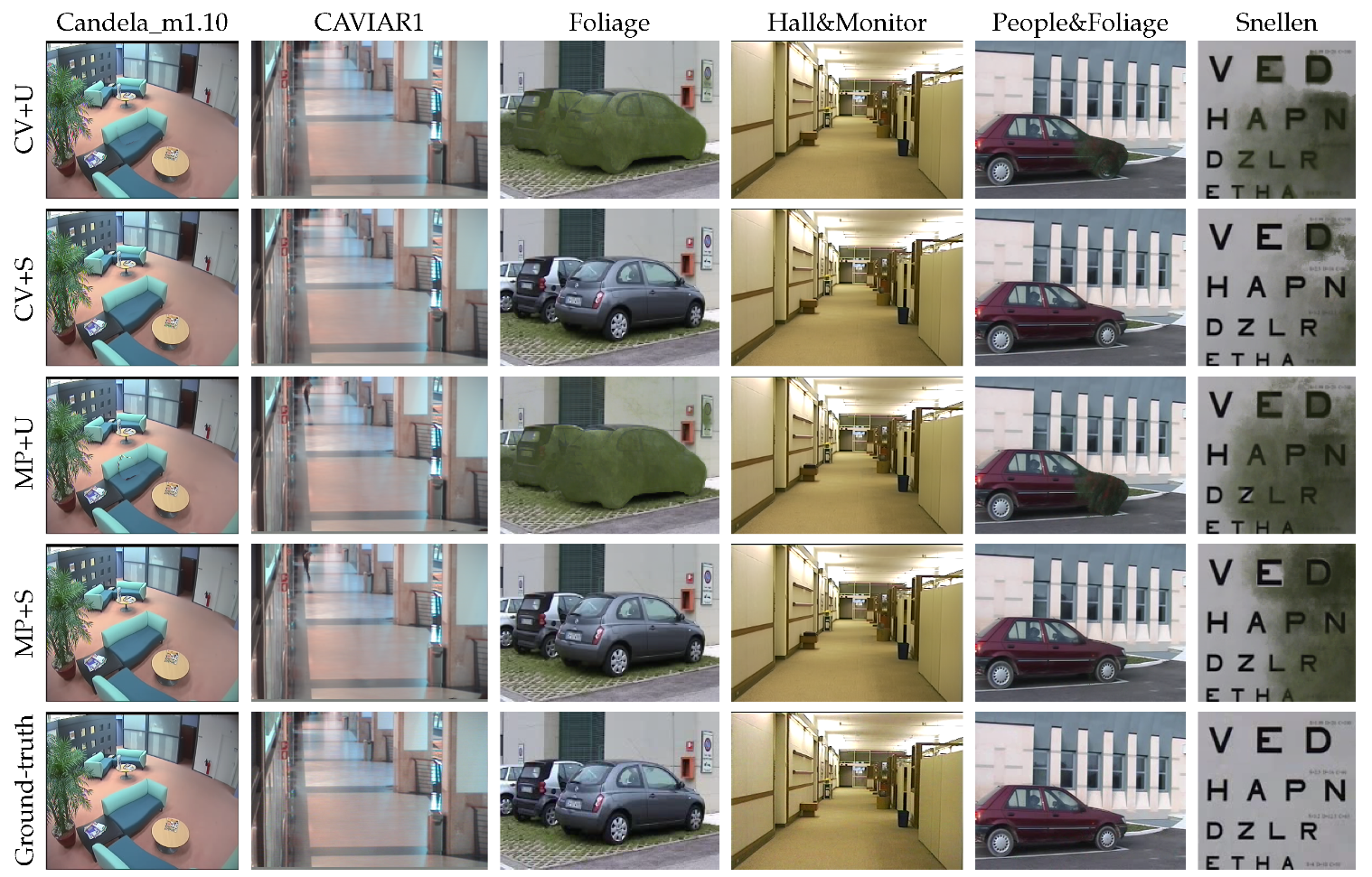
Figure 5 provides some background images generated by LaBGen-P-Semantic for each combination of methods and estimators for some SBI sequences. One can observe that, given a category of estimators, the difference between the backgrounds generated when using the CV and MP methods is barely noticeable. In “Foliage”, that is a video sequence in which parked cars are occluded by waving leaves, it is interesting to observe that the color of the leaves remains in front of the cars. Such a phenomenon can be explained by the fact that the probabilities $P\left(G=\mathrm{fg}\left|O=o_i\right.\right)$ obtained with the universal estimators are larger when $O=\mathrm{car}$ than when $O=\mathrm{plant}$. Thus, when observing the leaves, LaBGen-P-Semantic considers that there is less motion than when it observes the cars and selects the pixel intensities of the leaves.

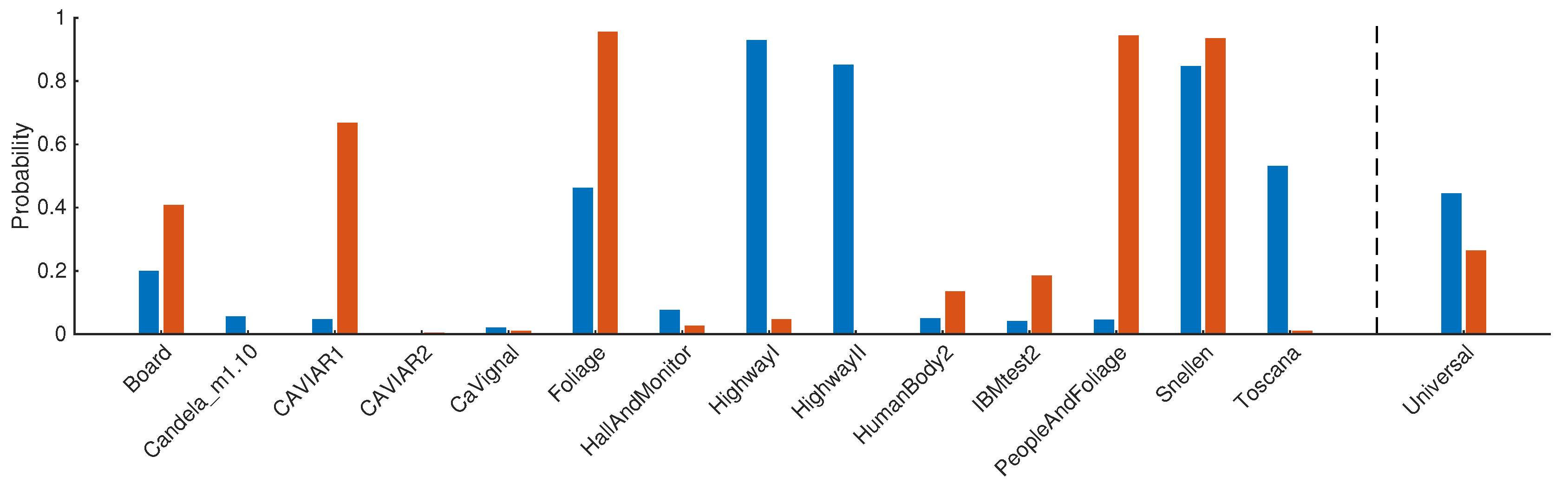
Figure 6 provides, for each video sequence of the SBI dataset, the probabilities $P\left(G=\mathrm{fg}\left|O=o_i\right.\right)$ with $O=\mathrm{car}$ and $O=\mathrm{plant}$ obtained using the CV scene-specific estimators. The probabilities obtained with the universal estimators applied on the universal training dataset are given, as well. One can observe that, depending on the video sequence, the probabilities when $O=\mathrm{car}$ should be less or larger than when $O=\mathrm{plant}$. The video sequence “Foliage” requires a probability $P\left(G=\mathrm{fg}\left|O=o_i\right.\right)$ larger when $O=\mathrm{plant}$ than when $O=\mathrm{car}$, which is not the case when the universal estimators are used. Although these observations reveal a current limitation of our universal estimators, resulting from the fact that the probabilities $P\left(G=\mathrm{fg}\left|O=o_i\right.\right)$ are similar and static for any video sequence, we show in the next experiment that LaBGen-P-Semantic with CV+U and MP+U achieves a state-of-the-art performance on a large dataset.

4.4. Performance Evaluation

In order to perform a comprehensive evaluation of LaBGen-P-Semantic on a large dataset and compare its average performance to other background generation methods, we applied our method on the SBMnet dataset. As we do not have enough data to apply scene-specific estimators on all the sequences of this dataset (see Section 4.1), we assess LaBGen-P-Semantic with CV+U and MP+U only. For this purpose, we find the set of parameters $\mathcal{N}\in \left\{1,2\dots ,50,\infty \right\}$ and $\mathcal{S}\in \left\{1,2,\dots ,201\right\}$ of LaBGen-P-Semantic with CV+U, which maximizes the CQM score averaged over the almost complete SBI+SBMnet-GT dataset (putting apart the very short video sequences). Using this dataset enables us to optimize the parameters of LaBGen-P-Semantic on the largest collection of video sequences for which ground-truth background images are available. It turns out that we obtained an average CQM score of $32.2311$dB with $\mathcal{N}=3$ and $\mathcal{S}=90$. Note that we reduce the parameter $\mathcal{S}$ to a specific parameter value ${\mathcal{S}}_{\mathrm{short}}=4$ for the very short sequences. Thus, we suggest the following default set of parameters for LaBGen-P-Semantic:

$${\left(\mathcal{N},\mathcal{S},{\mathcal{S}}_{\mathrm{short}}\right)}_{\mathrm{default}}=\left(3,90,4\right).$$

(27)

After applying LaBGen-P-Semantic with CV+U (resp. MP+U) and the default set of parameters on the complete SBMnet dataset (that shares, according to Table 1, 19 video sequences with SBI+SBMnet-GT), we submitted the results to the SBMnet web platform (http://scenebackgroundmodeling.net) and got the results presented in

Table 4. Top 10 reported on the SBMnet website 6 May 2018 in which the performance achieved by LaBGen-P-Semantic with CV+U is inserted (in red). “A. R.” stands for average ranking.

Method	A. R. Across	Average	Average	Average	Average	Average	Average	Average
	Categories ↓	Ranking ↓	AGE ↓	pEPs ↓	pCEPs ↓	MS-SSIM ↑	PSNR ↑	CQM ↑
LaBGen-OF [7]	$4.88$	$2.17$	$6.1897$	$5.66\%$	$2.32\%$	$0.9412$	$29.8957$	$30.7006$
MSCL [26]	$5.25$	$1.17$	$5.9545$	$5.24\%$	$1.71\%$	$0.9410$	$30.8952$	$31.7049$
BEWiS [27]	$6.50$	$4.33$	$6.7094$	$5.92\%$	$2.66\%$	$0.9282$	$28.7728$	$29.6342$
LaBGen [5]	$8.38$	$5.00$	$6.7090$	$6.31\%$	$2.65\%$	$0.9266$	$28.6396$	$29.4668$
LaBGen-P-Semantic (CV+U)	$8.38$	$7.67$	$7.3890$	$7.61\%$	$3.57\%$	$0.9267$	$28.5050$	$29.3829$
LaBGen-P [6]	$9.25$	$6.67$	$7.0738$	$7.06\%$	$3.19\%$	$0.9278$	$28.4660$	$29.3196$
Temporal median	$9.63$	$12.67$	$8.2761$	$9.84\%$	$5.46\%$	$0.9130$	$27.5364$	$28.4434$
SC-SOBS-C4 [28]	$10.63$	$9.00$	$7.5183$	$7.11\%$	$2.42\%$	$0.9160$	$27.6533$	$28.5601$
MAGRPCA [29]	$10.63$	$10.33$	$8.3132$	$9.94\%$	$5.67\%$	$0.9401$	$28.4556$	$29.3152$
TMFG [30]	$10.88$	$15.67$	$9.4020$	$10.51\%$	$5.66\%$	$0.9043$	$27.1347$	$28.0530$
Photomontage [31]	$11.88$	$7.67$	$7.1950$	$6.86\%$	$2.57\%$	$0.9189$	$28.0113$	$28.8719$

(resp.

Table 5. Top 10 reported on the SBMnet website 6 May 2018 in which the performance achieved by LaBGen-P-Semantic with MP+U is inserted (in red). “A. R.” stands for average ranking.

Method	A. R. Across	Average	Average	Average	Average	Average	Average	Average
	Categories ↓	Ranking ↓	AGE ↓	pEPs ↓	pCEPs ↓	MS-SSIM ↑	PSNR ↑	CQM ↑
LaBGen-OF [7]	$4.88$	$2.17$	$6.1897$	$5.66\%$	$2.32\%$	$0.9412$	$29.8957$	$30.7006$
MSCL [26]	$5.25$	$1.17$	$5.9545$	$5.24\%$	$1.71\%$	$0.9410$	$30.8952$	$31.7049$
BEWiS [27]	$6.63$	$4.33$	$6.7094$	$5.92\%$	$2.66\%$	$0.9282$	$28.7728$	$29.6342$
LaBGen [5]	$8.25$	$4.83$	$6.7090$	$6.31\%$	$2.65\%$	$0.9266$	$28.6396$	$29.4668$
LaBGen-P-Semantic (MP+U)	$8.75$	$9.17$	$7.9731$	$8.20\%$	$3.94\%$	$0.9212$	$28.3234$	$29.1992$
LaBGen-P [6]	$9.13$	$6.33$	$7.0738$	$7.06\%$	$3.19\%$	$0.9278$	$28.4660$	$29.3196$
Temporal median	$9.63$	$12.67$	$8.2761$	$9.84\%$	$5.46\%$	$0.9130$	$27.5364$	$28.4434$
MAGRPCA [29]	$10.63$	$10.00$	$8.3132$	$9.94\%$	$5.67\%$	$0.9401$	$28.4556$	$29.3152$
SC-SOBS-C4 [28]	$10.75$	$8.83$	$7.5183$	$7.11\%$	$2.42\%$	$0.9160$	$27.6533$	$28.5601$
TMFG [30]	$10.88$	$15.67$	$9.4020$	$10.51\%$	$5.66\%$	$0.9043$	$27.1347$	$28.0530$
Photomontage [31]	$11.88$	$7.67$	$7.1950$	$6.86\%$	$2.57\%$	$0.9189$	$28.0113$	$28.8719$

). Although the average ranking disagrees, the average ranking across categories considers that both evaluated methods improves the original LaBGen-P.

If we take a look at the ranking per category in

Table 6. Average ranking and CQM per category, reported on the SBMnet website, of LaBGen-P and LaBGen-P-Semantic with CV+U and MP+U. The best ranks and scores are indicated in bold, and the categories in which LaBGen-P-Semantic is ranked first on the SBMnet website are indicated in column “1st”. The results were submitted 6 May 2018.

		Average Ranking ↓				Average CQM ↑
Category	1st	CV+U	LaBGen-P	MP+U	LaBGen-P	CV+U	MP+U	LaBGen-P
Basic		$\mathbf{6}.\mathbf{33}$	$6.67$	$7.33$	$\mathbf{6}.\mathbf{50}$	$33.5776$	$33.5317$	$\mathbf{33}.\mathbf{8797}$
Intermittent Motion	✔	$\mathbf{1}.\mathbf{33}$	$3.83$	$\mathbf{2}.\mathbf{33}$	$3.83$	$\mathbf{33}.\mathbf{5830}$	$32.8462$	$32.7260$
Clutter		$\mathbf{5}.\mathbf{83}$	$9.33$	$\mathbf{5}.\mathbf{83}$	$9.33$	$\mathbf{30}.\mathbf{7288}$	$30.6027$	$29.1305$
Jitter		$8.83$	$\mathbf{6}.\mathbf{67}$	$9.83$	$\mathbf{6}.\mathbf{67}$	$26.0662$	$25.8366$	$\mathbf{26}.\mathbf{2834}$
Illumination Changes		$21.33$	$\mathbf{9}.\mathbf{17}$	$23.50$	$\mathbf{9}.\mathbf{17}$	$22.3803$	$21.6238$	$\mathbf{26}.\mathbf{3522}$
Background Motion	✔	$\mathbf{1}.\mathbf{00}$	$12.33$	$\mathbf{1}.\mathbf{00}$	$12.33$	$28.0108$	$\mathbf{28}.\mathbf{1119}$	$26.5748$
Very Long		$22.67$	$\mathbf{17}.\mathbf{50}$	$21.50$	$\mathbf{17}.\mathbf{83}$	$28.6867$	$\mathbf{29}.\mathbf{3482}$	$29.1409$
Very Short	✔	$\mathbf{1}.\mathbf{33}$	$11.33$	$\mathbf{1}.\mathbf{67}$	$11.33$	$\mathbf{32}.\mathbf{0297}$	$31.6927$	$30.4694$

, LaBGen-P-Semantic with CV+U (resp. MP+U) is ranked above LaBGen-P for 5 (resp. 4) categories over 8. With no surprise, LaBGen-P-Semantic becomes first in the “Intermittent Motion” category, the second method being RMR [32] with a rank of $3.67$ (resp. $3.50$) when the performance achieved with CV+U (resp. MP+U) is inserted. It is clear that leveraging semantic segmentation, which does not rely on temporal information, enables our method to improve the robustness against the inclusion of objects subject to intermittent motions in the background. Unlike traditional motion detection algorithms, the ones based on semantic segmentation are not sensible to bootstrapping and have no difficulty detecting a stopped object. Regarding the “Background Motion” category, LaBGen-P-Semantic becomes first, as well, thus preceding TMFG [30], which has a rank of $2.50$ when the performances of both methods are inserted. If we take the example of shimmering water, a motion detection based on semantic segmentation will have no difficulties detecting it as belonging to the background, while several traditional motion detection algorithms will produce many false motion positive classifications. Last, but not least, LaBGen-P-Semantic is also ranked first for the “Very Short” category, the second method being Photomontage [31] with a rank of $2.83$. This can be explained by the fact that leveraging semantic segmentation improves motion detection when abrupt transitions occur in a video sequence. Note that Table 6 shows that the main weaknesses of LaBGen-P-Semantic are illumination changes and camera jitter. This is due to the fact that there is still no intrinsic mechanism in LaBGen-P-Semantic to handle such events. Those observations are confirmed by the CQM scores also reported in Table 6.

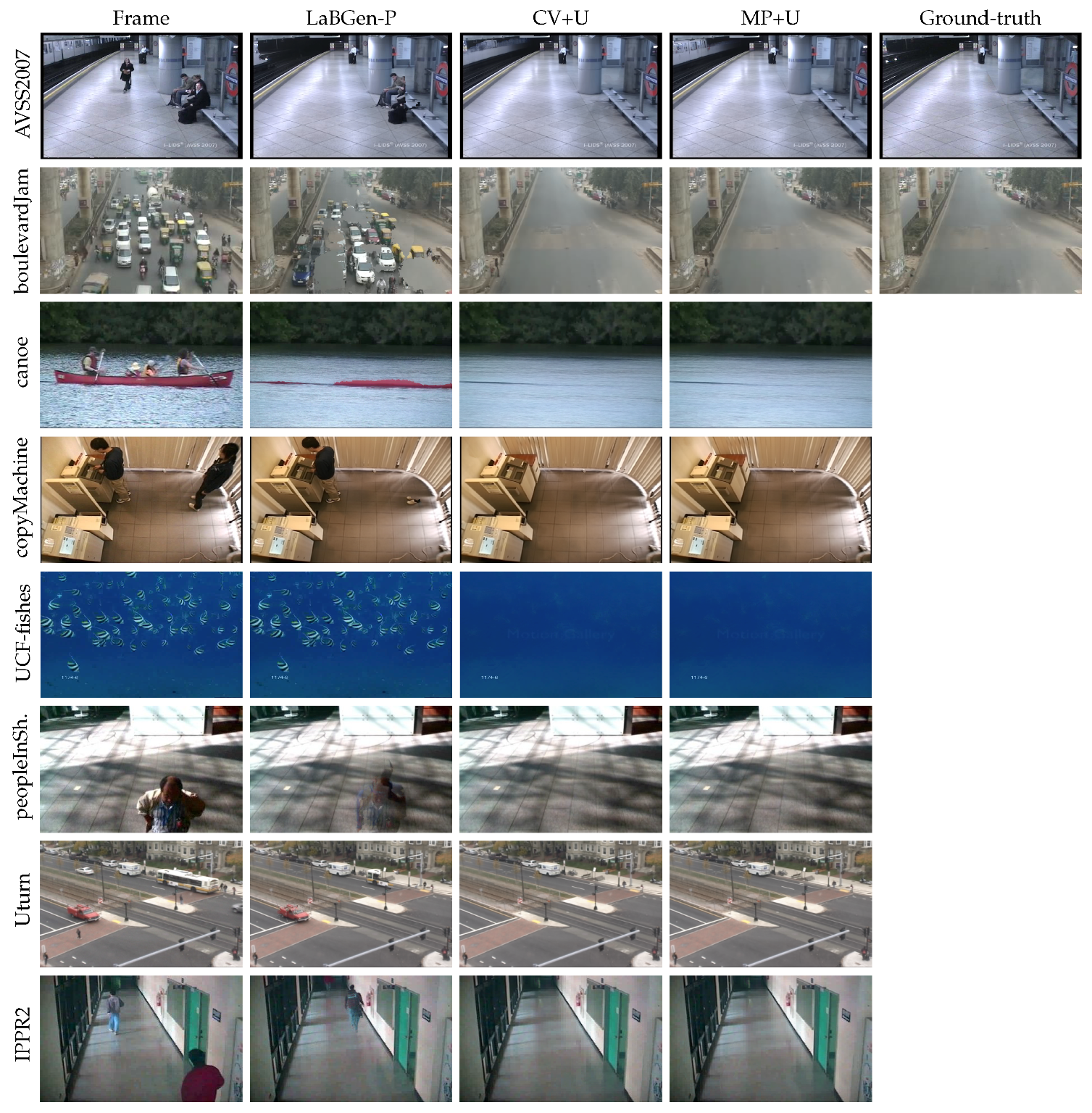
Finally, Figure 7 shows some SBMnet video sequences for which LaBGen-P-Semantic brought major improvements compared to LaBGen-P. Although those improvements are almost flawless, there are sometimes imperfections due to some limitations of the PSPNet algorithm that we observed during our experiments. First, obviously, this semantic segmentation algorithm cannot correctly segment objects that it never observed during its training. For instance, in “AVSS2007”, even though the persons on the bench are perfectly removed by LaBGen-P-Semantic, the metro, which is an object unknown by PSPNet, is still there. Second, the PSPNet algorithm has some intrinsic difficulties in segmenting very small objects. In some sequences, pedestrians are depicted by a few pixels, which can be difficult to interpret, even for the human eye. In “boulevardJam”, some pixel intensities depicting pedestrians are still present in the bottom-left corner of the generated background. Last, but not least, the PSPNet algorithm is not able to properly segment objects straddling the border of the image, such as a car leaving the scene. However, while leveraging semantic segmentation is not a perfect solution for background generation, our results show that we get state-of-the-art performances.

4.5. Performance Stability

For a user-specific video, there might be the need to fine-tune the parameters, subjectively, to produce the most suitable background image generated by LaBGen-P-Semantic. In such a situation, the default set of parameters given in Equation (27) might not suffice, and one could be interested in finding another set of parameters. In this section, we study the variation of performance with respect to the values given to our parameters. Following this study, we give some hints about the procedure to find new parameter values.

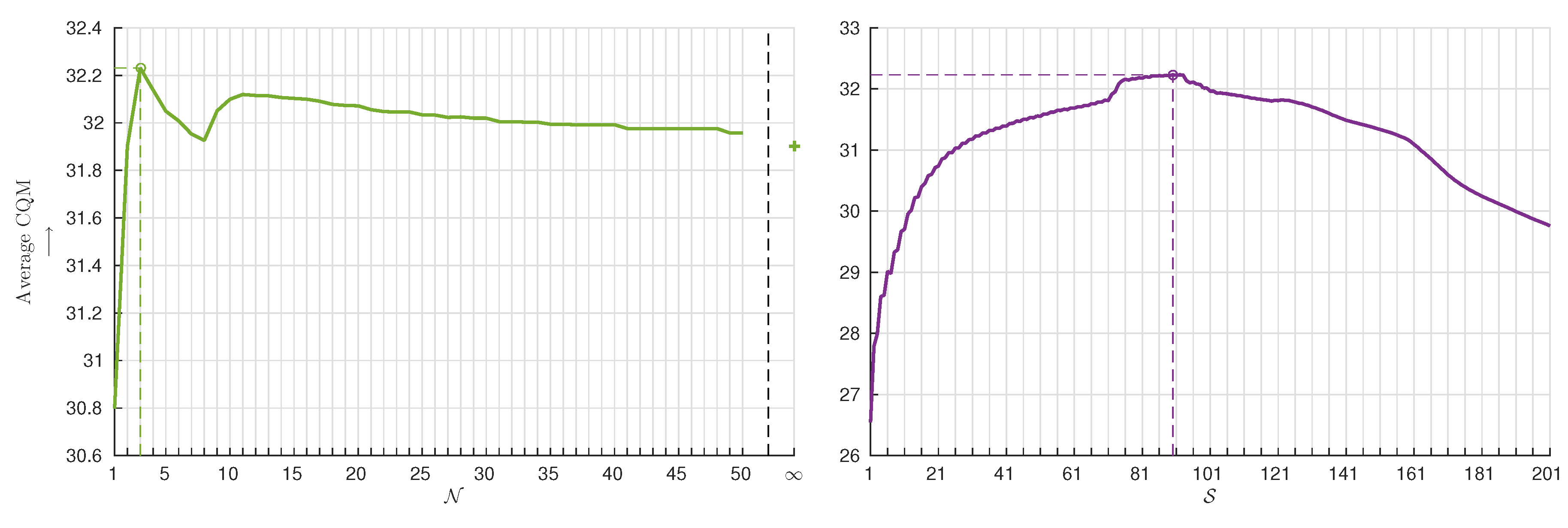
Figure 8 shows the performance stability, measured by the CQM, of LaBGen-P-Semantic with CV+U on the SBI+SBMnet-GT dataset. The parameters $\mathcal{N}$ and $\mathcal{S}$ vary around the default set of parameters proposed in Equation (27) ($\mathcal{N}=3$ and $\mathcal{S}=90$). Starting from the optimum, the average performance quickly decreases when the parameter $\mathcal{N}$ of the estimation step (see Section 2.2) drops. The case of $\mathcal{N}=1$, meaning that the size of the window used to aggregate motion scores is the smallest dimension of the input video sequence, is the worst regarding the associated CQM of $\simeq 30.8$dB. Furthermore, the average performance quickly decreases when $\mathcal{N}$ is increased from the optimum until $\mathcal{N}=8$. For $\mathcal{N}\in \left\{9,10,11\right\}$, the average performance increases. Afterwards, that is for $\mathcal{N}$ ranging from 12 to infinity, the performance slowly decreases. Thus, in situations where the default value for $\mathcal{N}$ seems not to be suitable, one should try to start finding an appropriate $\mathcal{N}$ from a large value and decrease it progressively.

Regarding the parameter $\mathcal{S}$ of the selection step (see Section 2.3), the average performance remains stable for $\mathcal{S}\in \left\{75,\dots ,94\right\}$. Outside this range, the average CQM score decreases faster when $\mathcal{S}$ tends to 1 than when it increases. The case of $\mathcal{S}=1$, meaning that a unique intensity is selected in each pixel location, is the worst given the associated CQM of $\simeq 26.5$dB. Note that an inappropriate value of $\mathcal{S}$ is more penalizing than an inappropriate value of $\mathcal{N}$. In conclusion, when the default value for $\mathcal{S}$ seems not to be appropriate, one should start by taking a large value of $\mathcal{S}$ and reduce it progressively, as we would do for finding $\mathcal{N}$.

5. Conclusions

In this paper, we presented LaBGen-P-Semantic, a background generation method, based on LaBGen-P, leveraging semantic segmentation in its motion detection step. Moreover, we presented two intra-frame methods for estimating motion from a semantic segmentation algorithm: CV, which computes, for a given pixel, the probability of observing an object belonging to the foreground, given the associated vector of scores; and MP, which is based on the hypothesis that computing the same probability, given the associated most probable object class, is similar. Computing those probabilities requires prior knowledge, which can be automatically estimated from a video sequence, or a dataset of video sequences. This estimation is made either with scene-specific estimators, enabling one to detect motion in video sequences captured in conditions similar to the processed video sequence; or universal estimators, enabling one to detect motion as well as possible in any video sequence.

Our experiments showed that, although the average performance achieved by LaBGen-P-Semantic with the MP method is slightly below the one with the CV method, our hypothesis is correct regarding the small gap between both. Thus, one is able to apply LaBGen-P-Semantic from a complete vector of scores or from semantic segmentation maps. Furthermore, using scene-specific estimators improves the average performance of LaBGen-P-Semantic compared to using universal ones. This can be explained by the fact that considering that an object belongs to the foreground depends on the content of the video sequence being processed. For instance, cars parked in a parking lot should be considered motionless, while cars on a highway should be considered in motion. Such considerations cannot be handled by leveraging the semantic segmentation alone.

In further experiments, we also showed that when evaluated on the large SBMnet dataset, LaBGen-P-Semantic with both CV+U and MP+U significantly improves LaBGen-P in several categories. Specifically, LaBGen-P-Semantic is ranked first among all the methods submitted to the SBMnet web platform in the “Intermittent Motion”, “Background Motion” and “Very Short” categories. Unlike traditional motion detection algorithms, leveraging semantic segmentation enables our method to avoid the inclusion of objects subject to intermittent motions in the background, the production of false motion positives due to a dynamic background and an inaccurate motion detection when abrupt transitions occur between consecutive frames. However, even though our results are not flawless in all categories, our first try at leveraging semantic segmentation for background generation confirms that using intra-frame motion detection is an appropriate choice for our method and paves the way for more methods based on semantic segmentation.

References

- Maddalena, L.; Petrosino, A. Background Model Initialization for Static Cameras. In Background Modeling and Foreground Detection for Video Surveillance; Chapman and Hall/CRC: Boca Raton, FL, USA, 2014; Chapter 3; pp. 114–129. [Google Scholar]
- Bouwmans, T.; Maddalena, L.; Petrosino, A. Scene Background Initialization: A Taxonomy. Pattern Recognit. Lett. 2017, 96, 3–11. [Google Scholar] [CrossRef]
- Jodoin, P.M.; Maddalena, L.; Petrosino, A.; Wang, Y. Extensive Benchmark and Survey of Modeling Methods for Scene Background Initialization. IEEE Trans. Image Process. 2017, 26, 5244–5256. [Google Scholar] [CrossRef] [PubMed]
- Laugraud, B.; Piérard, S.; Braham, M.; Van Droogenbroeck, M. Simple median-based method for stationary background generation using background subtraction algorithms. In Proceedings of the International Conference on Image Analysis and Processing (ICIAP), Workshop on Scene Background Modeling and Initialization (SBMI), Genoa, Italy, 7–11 September 2015; Lecture Notes in Computer Science. Springer: Berlin, Germany, 2015; Volume 9281, pp. 477–484. [Google Scholar]
- Laugraud, B.; Piérard, S.; Van Droogenbroeck, M. LaBGen: A method based on motion detection for generating the background of a scene. Pattern Recognit. Lett. 2017, 96, 12–21. [Google Scholar] [CrossRef] [Green Version]
- Laugraud, B.; Piérard, S.; Van Droogenbroeck, M. LaBGen-P: A Pixel-Level Stationary Background Generation Method Based on LaBGen. In Proceedings of the 23rd International Conference on IEEE International Conference on Pattern Recognition (ICPR), Cancún, Mexico, 4–8 December 2016; pp. 107–113. [Google Scholar]
- Laugraud, B.; Van Droogenbroeck, M. Is a Memoryless Motion Detection Truly Relevant for Background Generation with LaBGen? In Proceedings of the International Conference on Advanced Concepts for Intelligent Vision Systems (ACIVS), Antwerp, Belgium, 18–21 September 2017; Lecture Notes in Computer Science. Springer: Berlin, Germany, 2017; Volume 10617, pp. 443–454. [Google Scholar]
- Braham, M.; Piérard, S.; Van Droogenbroeck, M. Semantic Background Subtraction. In Proceedings of the IEEE International Conference on Image Processing (ICIP), Beijing, China, 17–20 September 2017; pp. 4552–4556. [Google Scholar]
- Zhao, H.; Shi, J.; Qi, X.; Wang, X.; Jia, J. Pyramid Scene Parsing Network. In Proceedings of the IEEE International Conference on Computer Vision and Pattern Recognition (CVPR), Honolulu, HI, USA, 21–26 July 2017; pp. 6230–6239. [Google Scholar]
- Bouwmans, T. Recent Advanced Statistical Background Modeling for Foreground Detection—A Systematic Survey. Recent Pat. Comput. Sci. 2011, 4, 147–176. [Google Scholar]
- Bouwmans, T. Subspace Learning for Background Modeling: A Survey. Recent Pat. Comput. Sci. 2009, 2, 223–234. [Google Scholar] [CrossRef]
- Bouwmans, T.; Sobral, A.; Javed, S.; Jung, S.K.; Zahzah, E.H. Decomposition into low-rank plus additive matrices for background/foreground separation: A review for a comparative evaluation with a large-scale dataset. Comput. Sci. Rev. 2017, 23, 1–71. [Google Scholar] [CrossRef] [Green Version]
- Sobral, A.; Javed, S.; Jung, S.K.; Bouwmans, T.; Zahzah, E.H. Online Stochastic Tensor Decomposition for Background Subtraction in Multispectral Video Sequences. In Proceedings of the International Conference on Computer Vision Workshops (ICCV Workshops), Santiago, Chile, 11–18 December 2015; pp. 946–953. [Google Scholar]
- Bouwmans, T. Background Subtraction for Visual Surveillance: A Fuzzy Approach. In Handbook on Soft Computing for Video Surveillance; Pal, S.K., Petrosino, A., Maddalena, L., Eds.; Taylor and Francis Group: Abingdon, UK, 2012; Chapter 5; pp. 103–138. [Google Scholar]
- Bouwmans, T. Traditional and recent approaches in background modeling for foreground detection: An overview. Comput. Sci. Rev. 2014, 11–12, 31–66. [Google Scholar] [CrossRef]
- Crow, F. Summed-area tables for texture mapping. In Proceedings of the 11th Annual Conference on Computer Graphics and Interactive Techniques SIGGRAPH, Minneapolis, MN, USA, 23–27 July 1984; Computer Graphics. ACM: New York, NY, USA, 1984; Volume 18, pp. 207–212. [Google Scholar]
- Zhou, B.; Zhao, H.; Puig, X.; Fidler, S.; Barriuso, A.; Torralba, A. Semantic understanding of scenes through the ADE20K dataset. arXiv 2016, arXiv:arXiv:1608.05442. [Google Scholar]
- Zhou, B.; Zhao, H.; Puig, X.; Fidler, S.; Barriuso, A.; Torralba, A. Scene Parsing through ADE20K Dataset. In Proceedings of the IEEE International Conference on Computer Vision and Pattern Recognition (CVPR), Honolulu, HI, USA, 21–26 July 2017; pp. 5122–5130. [Google Scholar]
- Maddalena, L.; Petrosino, A. Towards Benchmarking Scene Background Initialization. In Proceedings of the International Conference on Image Analysis and Processing Workshops (ICIAP Workshops), Genova, Italy, 7–11 September 2015; Volume 9281, pp. 469–476. [Google Scholar]
- Wang, Y.; Luo, Z.; Jodoin, P.M. Interactive Deep Learning Method for Segmenting Moving Objects. Pattern Recognit. Lett. 2017, 96, 66–75. [Google Scholar] [CrossRef]
- Goyette, N.; Jodoin, P.M.; Porikli, F.; Konrad, J.; Ishwar, P. changedetection.net: A New Change Detection Benchmark Dataset. In Proceedings of the IEEE International Conference on Computer Vision and Pattern Recognition Workshops (CVPRW), Providence, RI, USA, 16–21 June 2012. [Google Scholar]
- Wang, Y.; Jodoin, P.M.; Porikli, F.; Konrad, J.; Benezeth, Y.; Ishwar, P. CDnet 2014: An Expanded Change Detection Benchmark Dataset. In Proceedings of the IEEE International Conference on Computer Vision and Pattern Recognition Workshops (CVPRW), Columbus, OH, USA, 23–28 June 2014; pp. 393–400. [Google Scholar]
- Wang, Z.; Simoncelli, E.P.; Bovik, A.C. Multiscale structural similarity for image quality assessment. In Proceedings of the Asilomar Conference on Signals, Systems and Computers, Pacific Grove, CA, USA, 9–12 November 2003; Volume 2, pp. 1398–1402. [Google Scholar]
- Wang, Z.; Bovik, A.C.; Sheikh, H.R.; Simoncelli, E.P. Image quality assessment: From error visibility to structural similarity. IEEE Trans. Image Process. 2004, 13, 600–612. [Google Scholar] [CrossRef] [PubMed]
- Yalman, Y.; Ertürk, I. A new color image quality measure based on YUV transformation and PSNR for human vision system. Turk. J. Electr. Eng. Comput. Sci. 2013, 21, 603–613. [Google Scholar]
- Javed, S.; Mahmood, A.; Bouwmans, T.; Jung, S.K. Background-Foreground Modeling Based on Spatiotemporal Sparse Subspace Clustering. IEEE Trans. Image Process. 2017, 26, 5840–5854. [Google Scholar] [CrossRef] [PubMed]
- De Gregorio, M.; Giordano, M. Background estimation by weightless neural networks. Pattern Recognit. Lett. 2017, 96, 55–65. [Google Scholar] [CrossRef]
- Maddalena, L.; Petrosino, A. Extracting a Background Image by a Multi-modal Scene Background Model. In Proceedings of the 23rd International Conference on IEEE International Conference on Pattern Recognition (ICPR), Cancún, Mexico, 4–8 December 2016; pp. 143–148. [Google Scholar]
- Javed, S.; Mahmmod, A.; Bouwmans, T.; Jung, S.K. Motion-Aware Graph Regularized RPCA for Background Modeling of Complex Scene. In Proceedings of the IEEE International Conference on Pattern Recognition (ICPR), Cancún, Mexico, 4–8 December 2016; pp. 120–125. [Google Scholar]
- Liu, W.; Cai, Y.; Zhang, M.; Li, H.; Gu, H. Scene Background Estimation Based on Temporal Median Filter with Gaussian Filtering. In Proceedings of the IEEE International Conference on Pattern Recognition (ICPR), Cancún, Mexico, 4–8 December 2016; pp. 132–136. [Google Scholar]
- Agarwala, A.; Dontcheva, M.; Agrawala, M.; Drucker, S.; Colburn, A.; Curless, B.; Salesin, D.; Cohen, M. Interactive Digital Photomontage. ACM Trans. Graph. 2004, 23, 294–302. [Google Scholar] [CrossRef]
- Ortego, D.; SanMiguel, J.M.; Martínez, J.M. Rejection based multipath reconstruction for background estimation in video sequences with stationary objects. Comput. Vis. Image Underst. 2016, 147, 23–37. [Google Scholar] [CrossRef]
Figure 1.
Example of a pixel marked by a red cross in the white car of the image (a) along with its 20 over 150 largest scores (b) returned by the PSPNet algorithm [9] (see Section 4.1).
Figure 2.
Example of a frame (a) along with its semantic segmentation map (b) returned by the PSPNet algorithm [9] (see Section 4.1) and an alpha blending of both (c). The labels are: road ■, grass ■, sidewalk ■, earth ■, plant ■, car ■ and fence ■.
Figure 3.
Illustration of the difference between a motion map and a segmentation map. The absolute difference of pixel intensities between frames (a) and (b) results in the motion map (c). Producing the segmentation map (d) requires finding an appropriate hard threshold (set to 25 for the example) and prevents knowing how large the difference of pixel intensities is.
Figure 4.
Illustration of the difference between motion scores and quantities of motion. The absolute difference of pixel intensities between frames (a) and (b) results in the motion map (c). The estimation step applied on this motion map for is displayed in (d). For the purpose of visualization, the quantities of motion in (d) have been normalized with respect to the largest quantity in the frame.
Figure 5.
Backgrounds generated by LaBGen-P-Semantic with and for the video sequences of the SBI dataset with CV+U (1st row), CV+S (2nd row), MP+U (3rd row) and MP+S (4th row). We provide generated backgrounds, along with the corresponding ground-truth (5th row), only for video sequences in which differences are noticeable.
Figure 6.
Probabilities with ■, and ■ , obtained using the CV scene-specific estimators for each sequence of the SBI dataset and the CV universal estimators applied on the universal training dataset (see Section 4.2).
Figure 7.
Visual results showing some major improvements brought by LaBGen-P-Semantic with CV+U and MP+U on some SBMnet video sequences. A random frame of the input video sequence along with the ground-truth (when available) are also provided.
Figure 8.
Average performance of LaBGen-P-Semantic with CV+U on the SBI+SBMnet-GT dataset when the parameters and vary around the default set of parameters proposed in Equation (27). The best average performance is indicated by a circle.