Adaptive Multi-Scale Entropy Fusion De-Hazing Based on Fractional Order

Abstract

This paper describes a proposed fractional filter-based multi-scale underwater and hazy image enhancement algorithm. The proposed system combines a modified global contrast operator with fractional order-based multi-scale filters used to generate several images, which are fused based on entropy and standard deviation. The multi-scale-global enhancement technique enables fully adaptive and controlled color correction and contrast enhancement without over exposure of highlights when processing hazy and underwater images. This in addition to the illumination/reflectance estimation coupled with global and local contrast enhancement. The proposed algorithm is also compared with the most recent available state-of-the-art multi-scale fusion de-hazing algorithm. Experimental comparisons indicate that the proposed approach yields a better edge and contrast enhancement results without a halo effect, without color degradation, and is faster and more adaptive than all other algorithms from the literature.

1. Introduction

Hazy and underwater images share similar characteristics in terms of reduced visibility and low contrast due to the nature of image formation [1,2]. Several single image-based enhancement and restoration models and algorithms have been proposed to solve this problem [1,2]. However, they work with varying degrees of success at the cost of increased structural and computational complexity. Furthermore, color correction combined with these highly complex de-hazing algorithms have been used to restore underwater images. However, there are relatively few digital hardware realizations and reduced real-time prospects for such schemes due to a high computational cost.

In this work, we propose a fractional order-based algorithm for the enhancement of hazy and underwater images. The algorithm performs color correction and multiscale spatial filter-based localized enhancement. We compare results with other algorithms from the literature and show that the proposed system is effective with the fastest execution time.

The paper is outlined as follows. The Section 2 provides the background, motivation, and key contributions of the proposed system. Section 3 presents the proposed algorithms for both underwater and hazy image enhancement in addition to solutions to problems and modifications. Section 4 presents and compares the results (obtained using the proposed system) to other algorithms from the literature. The Section 5 explicitly compares the proposed approach against a recent algorithm from the literature, which further strengthens the justification of the proposed scheme. The Section 6 presents the conclusion.

2. Materials and Methods

2.1. Underwater Image Processing Algorithms

Underwater image processing algorithms can be classified as either restoration, enhancement, or color correction and illumination of normalization-based approaches [2] and range from medium to high computational and structural complexity. The restoration-based algorithms incorporate de-blurring and de-hazing processes using either Weiner [3] deconvolution or dark channel prior (DCP)-based techniques, respectively [2]. Examples include algorithms by Galdran et al. [4], Li et al. [5], Guo [6], Zhao et al. [7], Chiang and Chen [8], Wen et al. [9], Serikawa and Lu [10], Carlevaris-Bianco et al. [11], and Chiang et al. [12]. Conversely, the enhancement-based algorithms do not employ any models derived from physical phenomena or prior image information [2]. They utilize statistical/histogram-based or logarithmic contrast enhancement/stretching and color correction techniques in their formulation. Examples include works by Iqbal et al. [13], Ghani and Isa [14], Fu et al. [15], Gouinaud et al. [16], Bazeille et al. [17], Chambah et al. [18], Torres-Mendez and Dudek [19], Ahlen et al. [20,21], Petit et al. [22], Bianco et al. [23], Prabhakar et al. [24], Lu et al. [25], and Li et al. [5]. Recently, entropy and gradient optimized underwater image processing algorithms based on partial differential equations were developed [26,27] and they yielded effective and automated enhancement surpassing results from previous algorithms.

The illumination normalization-based algorithms attempt to resolve uneven lighting issues in the acquired underwater image scenes. The algorithms in this class include works by Prabhakar et al. [24], Garcia et al. [28], Rzhanov et al. [29], Singh et al. [30], and Fu et al. [15].

2.2. Hazy Image Processing Algorithms

Hazy image processing also deals with visibility restoration of image scenes degraded by weather conditions and can be multi-image or single-image based solutions [31]. Furthermore, hazy image processing algorithms can also be classified as either restoration or enhancement-based schemes. In the restoration-based hazy image processing, the de-hazing process is based on the hazy image formation model [31]. The objective is, therefore, meant to obtain the de-hazed image from the input hazy image. The algorithms in this class include the popular DCP method by He et al. [32], which has been adopted and modified in various forms and a review of several DCP-based methods can be found in Reference [1].

Other schemes include works based on segmentation [33,34,35], fusion [36,37], geometry [38], Weighted Least Squares [39], variational [37,40,41,42], and regularization approaches [34] using sparse priors [43], other boundary constraints [44], biological retina-based model [45], and multi-scale convolutional neural networks [46]. The enhancement-based hazy image processing method is based on directly obtaining the by-product of radiance scene recovery through visibility restoration by contrast enhancement/maximization. The algorithms in this category utilize contrast limited adaptive histogram equalization (CLAHE), histogram specification (HS) [47], and Retinex [48,49,50]. Additionally, some of these algorithms combine dark channel priors and transmission map extraction with contrast enhancement for refinement. However, consistently good results are not guaranteed since some images will depict color fading/distortion and darkening of regions in addition to over-enhancement of sky/homogeneous regions. Thus, some threshold and segmentation-based algorithms [33,34,35,51] have been developed to solve the peculiar problems of these algorithms. Furthermore, recently developed algorithms using partial differential equations (PDEs) and gradient metric-based optimization were developed [52,53] to avoid the usage of DCP-based stages and multiple (and manual adjustment of) parameters. Recently, an Artificial Multiple-Exposure Image Fusion (AMEF) de-hazing algorithm was proposed by Galdran [54], which represents the current state-of-the-art technology.

Other recent algorithms utilize hybrid methods, deep learning, and convolutional neural network architectures for de-hazing and include works by References [55,56,57,58,59,60,61,62,63,64,65,66,67,68,69,70,71,72,73].

Physical methods depend on prior image information obtained by capturing the image scenes at different times under varying conditions using physical hardware/optical equipment such as cameras and lighting rigs [2]. They may also incorporate multi-image processing schemes for either hazy or underwater images. However, consistently good results are not assured due to the unpredictable nature of weather and aquatic medium conditions. In addition, the cost of such hardware imaging systems is prohibitive and are usually not universally applicable. Such schemes are fully listed and described in work by Li et al. [5]. Single-image-based software implementations offer the best outcome when factors such as cost, time, replicability, and convenience are considered since they do not necessarily require prior knowledge of the environment or an image acquisition process for operation [2,5]. Thus, the scope of this work is limited to single-image-based enhancement of both hazy and underwater images.

The primary motivation for this work is to develop fast, practical, and effective algorithms for underwater and hazy image enhancement that are amenable to hardware implementation for real-time operation.

2.3. Key Contributions and Features of a Proposed Scheme

The key contributions and features of this work include:

• A modified global contrast enhancement and a multi-scale illumination/reflectance model-based algorithm using fractional order calculus-based kernels.
• Relatively low-complexity underwater image enhancement algorithm utilizing color correction and contrast operators.
• Frequency-based approach to image de-hazing and underwater image enhancement using successive, simultaneous high frequency component augmentation and low frequency component reduction.
• Feasible hazy and underwater image enhancement algorithm for relatively easier hardware architecture implementation.
• Avoidance of the dark channel prior based stages and iterative schemes by utilizing combined multi-level convolution using fractional derivatives.

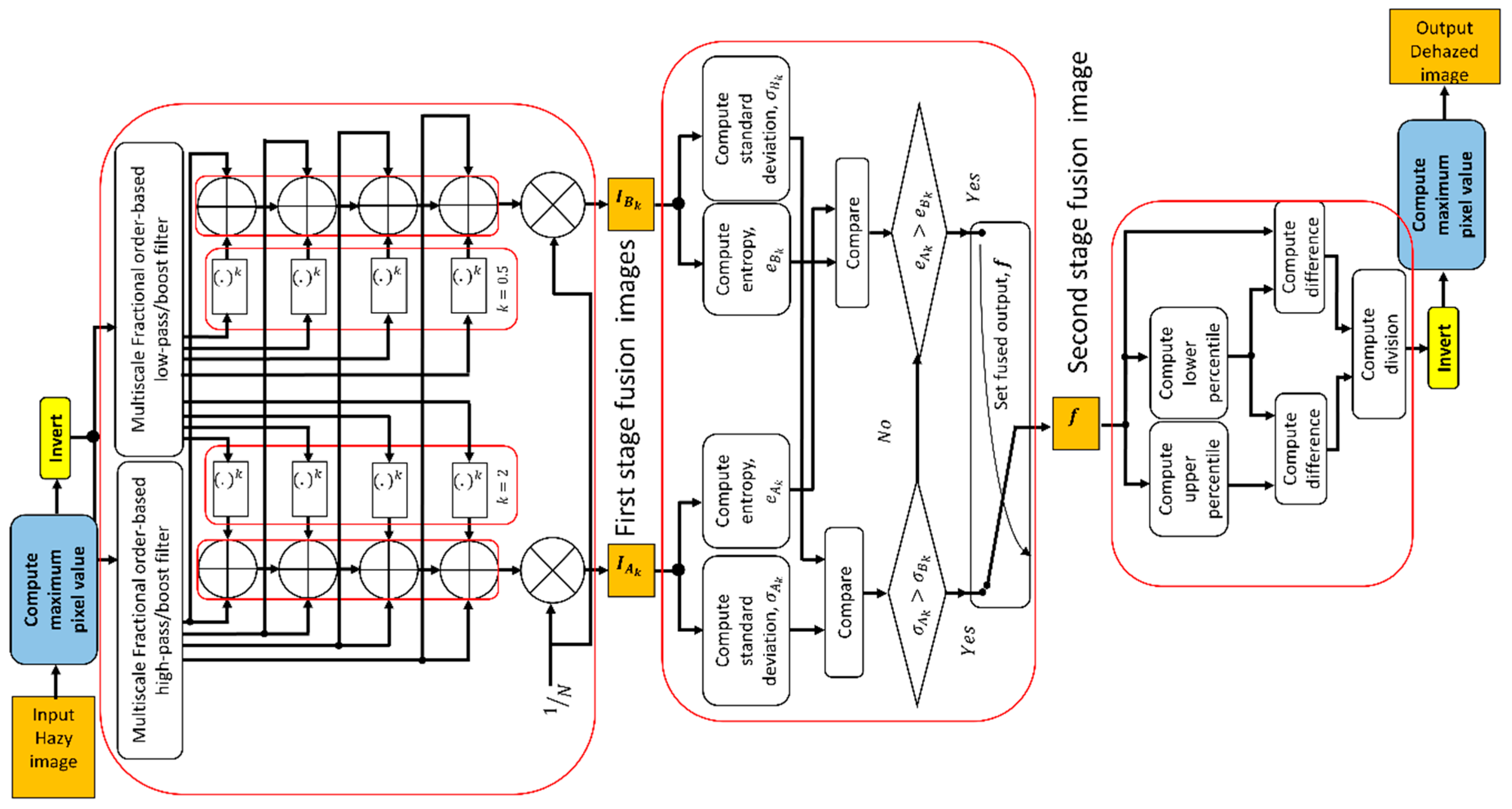
3. Proposed Algorithms

Underwater image enhancement usually involves some color correction/white balancing in addition to contrast enhancement process, which is usually a local/global operation. The first step for reducing the need for such involved local processing was to avoid the over-exposure of bright regions while enhancing the dark regions. Initial logarithmic solutions were ineffective and flattened the images in addition to fading colors. Thus, a new formulation for the global contrast operator had to be devised to achieve this objective. We present the modification and realization of the improved global contrast operator and spatial filter based system for processing underwater and hazy images. Furthermore, the simplified scheme using fractional calculus is presented in the form of spatial masks based on the Grunwald-Letnikov definition [74].

3.1. Selection and Modification of Global Contrast Operator

Previously, extensive experiments were conducted to determine effectiveness on several contrast stretching algorithms [26]. Due to the adjustable nature of the high and low values by modifying the percentiles, the contrast stretching (CS) algorithm appeared to be much more versatile than the other algorithms. However, it works best for faded low-contrast images but not so well for underwater images since it does not perform adequate color correction unless applied iteratively. Conversely, some of the other algorithms were too harsh and had no effect or minimal impact on most underwater images while others resulted in color bleeding. The selected algorithms such as the piecewise linear transform (PWL) [75] and the gain offset correction (GOC2) [76] were selected for incorporation into effective PDE-based formulations [26,27]. This was because some underwater images responded better to GOC2 (due to its mainly color correction ability) than to PWL (due to its generality) and vice versa. Thus, there is the need to develop a global contrast operator that would merge the advantages of both GOC2 and PWL while mitigating their weaknesses.

Since the linear contrast stretch (similar to the PWL and GOC2) does not utilize any edge enhancement features or region-based methods, it does not enhance noisy edge artefacts. However, several of these contrast stretching algorithms lead to oversaturation of already bright regions of the image (whitening out/over-exposure). This is in addition to a threshold effect when applied to images with bimodal histogram. The linear contrast stretching can be applied to both greyscale and color images with excellent results similar to the PWL. However, the PWL method also suffers from the threshold of images when there are distinct regions of dark and light intensity, which leads to whiting out of bright areas. This is because it truncates values at upper and lower limits to maximum and minimum possible pixel values in the image without taking into account pixels in those regions. The linear contrast stretch seeks to expand the range based on the surrounding pixels in the distribution.

Underwater image enhancement usually involves some color correction/white balancing in addition to contrast enhancement process, which is usually a local/global operation. The GOC2 algorithm adequately processed underwater images, which required mild color correction and contrast enhancement and, thus, avoided overexposure of highlights unlike most other tested contrast enhancement algorithms [26]. This necessitated the incorporation of a local contrast operator such as the CLAHE, which, even though effective, further added to the computational complexity of the algorithms and introduced additional parameters. The first step to reducing the need for such involved local processing was to avoid the over-exposure of bright regions while enhancing the dark regions. Initial logarithmic solutions were not effective and flattened the images in addition to fading colors. Thus, a new formulation for the global contrast operator had to be devised to achieve this objective.

3.1.1. Gain Offset Correction-Based Stretching (GOCS)

The expression for the GOC2 mapping function [76] is given as shown in Equation (1).

$$I_{o_{GOC2}}=\left[\frac{L-1}{I_{max}-I_{min}}\right]\left(I_i-I_{min}\right)$$

(1)

The contrast stretching function is given below.

$$I_{o_{CS}}=\left[\frac{I_{max}-I_{min}}{I_{high}-I_{low}}\right]\left(I_i-I_{low}\right)+I_{min}$$

(2)

In Equations (1) and (2), $I_{o_{GOC2}}$ and $I_{o_{CS}}$ are the enhanced images using GOC2 and CS respectively, $I_{max}$, $I_{min}$ are maximum and minimum pixel intensities in the input image, $I_i$, $L$ is the number of grey intensity levels ($L$ = 256 for unsigned integer, eight-bit-per-pixel (uint8, 8 bpp) image format) while $I_{low}$ and $I_{high}$ are the lower and upper percentiles of the image pixel intensity distribution normally set at 5% and 95%, respectively.

The faults of the GOC2 lie in the statistics such as maximum and minimum pixel intensity values utilized in its computation. Since an image, which is already utilizing its full dynamic range, will not be affected by such statistics, we needed to realize a more influential statistic. The contrast stretching operator utilizes lower and upper percentiles of the image intensity distribution for its computation. Consequently, the contrast stretching operator does not suffer over-exposure effects and performs adequate contrast enhancement. Conversely, the GOC2 performs sufficient color correction but minimal contrast enhancement. Thus, by replacing the maximum and minimum pixel intensity values with the upper and lower percentiles in the formulation, we can realize a new formula for the global contrast operation as seen in the equation below.

$$I_{o_{GOCS}}=\left[\frac{L-1}{I_{high}-I_{low}}\right]\left(I_i-I_{low}\right)$$

(3)

Initial experiments using the 5th and 95th percentiles led to some pixels being over-exposed and, as we widened the range between the percentiles, the results improved and, in some cases, settled on the 1st and 99th percentiles for the best results. Increasing the range to its maximum yields a result similar to GOC2, which is expected since the high and low percentiles now become the maximum and minimum pixel intensity values. The GOCS is related to the CS in the following form.

$$I_{o_{CS}}=I_{o_{GOCS}}\left(I_{max}-I_{min}\right)+I_{min}$$

(4)

3.2. Proposed Multi-Scale Local Contrast Operator

We present the development of the multi-scale algorithm for local contrast enhancement, which replaces the CLAHE used in previous work by drastically reducing complexity and run-time. The initial derivations of the illumination-reflectance estimation part of the algorithm using integer-based low-pass and high-pass filters can be found in previous work [2]. We focus on new aspects such as multi-scale, fractional order-based entropy and standard deviation guided enhancement.

3.2.1. Multi-Scale Fractional Order-Based Illumination/Reflectance Contrast Enhancement (Multi-fractional-IRCES)

The fractional derivative-based re-definitions for high-pass and low-pass filtering of arbitrary order $\alpha$ are obtained using the equations below.

$$I_{HPF}\left(x,y\right)=-{\nabla }^{\alpha }I\left(x,y\right)$$

(5)

and

$$I_{LPF}\left(x,y\right)={{\displaystyle \int }}_{\mathsf{\Omega }}^{}{I}_{HPF}\left(x,y\right)d\mathsf{\Omega }=-{{\displaystyle \int }}_{\mathsf{\Omega }}^{}{\nabla }^{\alpha }I\left(x,y\right)d\mathsf{\Omega }=I\left(x,y\right)+{\nabla }^{\alpha }I\left(x,y\right)$$

(6)

Leading to the expression using fractional order as seen in Equation (7) below.

$$I_e\left(x,y\right)=-{\nabla }^{\alpha }I\left(x,y\right)+{\left[I\left(x,y\right)+{\nabla }^{\alpha }I\left(x,y\right)\right]}^k$$

(7)

We further extend the application to hazy image enhancement as seen in the equations below.

$$U\left(x,y\right)=I_{max}-I\left(x,y\right)$$

(8)

$$U_e^{\alpha }\left(x,y\right)=-{\nabla }^{\alpha }U\left(x,y\right)+{\left[-{{\displaystyle \int }}_{\mathsf{\Omega }}^{}{\nabla }^{\alpha }U\left(x,y\right)d\mathsf{\Omega }\right]}^k$$

(9)

$$I_e^{\alpha }\left(x,y\right)=U_{e_{max}}^{\alpha }-U_e^{\alpha }\left(x,y\right)$$

(10)

In the expressions of Equations (5)–(10), $k$ is the power factor, $U\left(x,y\right)$ is the inverted image, $I_{max}$ is the maximum pixel intensity of the input image, $I\left(x,y\right)$, ${\nabla }^{\alpha }U\left(x,y\right)$ is the fractional derivative of the inverted image, and ${{\displaystyle \int }}_{\mathsf{\Omega }}^{}{\nabla }^{\alpha }U\left(x,y\right)d\mathsf{\Omega }$ denotes the fractional order integral. Additionally, $U_e^{\alpha }\left(x,y\right)$ is the enhanced inverted image using fractional order-based operations and $U_{e_{max}}^{\alpha }$ is the maximum pixel intensity of $U_e^{\alpha }\left(x,y\right)$ while $I_e^{\alpha }\left(x,y\right)$ is the de-hazed image using fractional order-based operations. Additionally, we wish to reduce the computational load of computing both the derivative and the integral especially in the fractional order-based version. Thus, we simple obtain the fractional integral of the input image and subtract it from the original image and multiply by the appropriate factor to obtain the fractional order derivative. This saves resources especially on digital hardware implementations since only one operator is utilized and re-used. This is easily expressed as the equations below.

$$I_{HPF}\left(x,y\right)=I\left(x,y\right)-I_{LPF}\left(x,y\right)$$

(11)

$$I_o\left(x,y\right)=\gamma \left[I\left(x,y\right)-I_{LPF}\left(x,y\right)\right]+{\left[I_{LPF}\left(x,y,t\right)\right]}^k$$

(12)

which gives the expressions using fractional order calculus as seen below.

$$I_o\left(x,y\right)=\gamma \left[I\left(x,y\right)-\left\{{{\displaystyle \int }}_{\mathsf{\Omega }}^{}{\nabla }^{\alpha }I\left(x,y\right)d\mathsf{\Omega }\right\}\right]+{\left[{{\displaystyle \int }}_{\mathsf{\Omega }}^{}{\nabla }^{\alpha }I\left(x,y\right)d\mathsf{\Omega }\right]}^k$$

(13)

The scheme for hazy image enhancement can also be updated accordingly without much effort. The central idea is that, by further decomposing a low-pass filtered image and enhancing the details at each level and recombining the results, we would obtain much finer local enhancement. Additionally, using the fractional order reduces or minimizes the issue of noise enhancement as high frequency components are amplified at each stage, which further reduces or minimizes the low frequency components at each stage. Since the haze is a low frequency phenomenon, we expect that such effects would be greatly reduced after processing without enhancing noise. The entropy and standard deviation measures are utilized to select the best outcome for the processed image in terms of the value of the exponent, k. The mathematical expressions for the algorithm are shown in Equations (14)–(20).

$$I_i\left(x,y\right)=I_{HPF}{}_i\left(x,y\right)+{\left[I_{LPF}{}_i\left(x,y\right)\right]}^k;i=0,1,\dots ,N-1$$

(14)

$$I_{A_k}\left(x,y\right)=\frac{1}{N}{\displaystyle \sum }_{i=0}^{N-1}{I}_i\left(x,y\right);k=2$$

(15)

$$I_{B_k}\left(x,y\right)=\frac{1}{N}{\displaystyle \sum }_{i=0}^{N-1}{I}_i\left(x,y\right);k=0.5$$

(16)

$$e_{A_k}=entropy\left(I_{A_k}\right);e_{B_k}=entropy\left(I_{B_k}\right)$$

(17)

$${\sigma }_{A_k}=std\left(I_{A_k}\right);{\sigma }_{B_k}=std\left(I_{B_k}\right)$$

(18)

$$\mathrm{f}\left(\mathrm{x},\mathrm{y}\right)=\{\begin{array}{c}{\mathrm{I}}_{{\mathrm{A}}_{\mathrm{k}}}\left(\mathrm{x},\mathrm{y}\right),|{\mathrm{e}}_{{\mathrm{A}}_{\mathrm{k}}}>{\mathrm{e}}_{{\mathrm{B}}_{\mathrm{k}}}\mathrm{or}{\mathsf{\sigma }}_{{\mathrm{A}}_{\mathrm{k}}}>{\mathsf{\sigma }}_{{\mathrm{B}}_{\mathrm{k}}}\\ {\mathrm{I}}_{{\mathrm{B}}_{\mathrm{k}}}\left(\mathrm{x},\mathrm{y}\right),|{\mathrm{e}}_{{\mathrm{A}}_{\mathrm{k}}}<{\mathrm{e}}_{{\mathrm{B}}_{\mathrm{k}}}\mathrm{or}{\mathsf{\sigma }}_{{\mathrm{A}}_{\mathrm{k}}}<{\mathsf{\sigma }}_{{\mathrm{B}}_{\mathrm{k}}}\end{array}$$

(19)

$$f_o\left(x,y\right)=GOCS\left[f\left(x,y\right)\right]$$

(20)

In Equation (14), $I_i\left(x,y\right)$ is the enhanced image at level $i$ and $N$ is the number of decomposition levels while $I_{HPF}{}_i\left(x,y\right)$ and $I_{LPF}{}_i\left(x,y\right)$ are high-pass and low-pass filtered images obtained at level $i$. Based on experiments, we set $N=5$. The obtained level images are then aggregated to obtain the final images $I_{A_k}$ or $I_{B_k}$ for the different values of the power factor and $k$ in Equations (15) and (16). The values for the power factor are chosen to be multiples of two (2) due to hardware design considerations to enable fast computation by bit shifting. This is explained by the fact that the value 0.5 is a multiple of 2 since 2ⁿ for n = −1; 2⁻¹ = ½ = 0.5 or 000.1. This is a right bit shift by one-bit position in binary logic for the binary representation of one (1) as 001.0. Conversely 2ⁿ for n = 1; 2¹ = 2, or 010.0. This makes the operation synthesizable for digital hardware realization since exponential operations become bit shifting operations, which are much faster.

The respective entropies ($e_{A_k}$, $e_{B_k}$) and standard deviations (${\sigma }_{A_k}$, ${\sigma }_{B_k}$) of the aggregated images are computed in Equations (17) and (18) and used to decide the best image outcome, $f\left(x,y\right)$ in Equation (19), which is then processed with the modified global contrast enhancement algorithm to obtain the final output image, $f_o\left(x,y\right),$ in Equation (20). This is based on the simultaneous multi-level high frequency component (edges and details) enhancement and multi-level low frequency component (haze) attenuation.

The diagram of the proposed algorithm for enhancement of both hazy and underwater images is shown in Figure 1. All processing operations are achieved with spatial filter kernels using fractional order-based calculus, which yields better results than the integer order in terms of balanced edge enhancement.

3.2.2. Preliminary Results

After testing several images, it was discovered that some images were better enhanced when using the 5th and 95th percentiles rather than the 1st and 99th percentiles. The representative images of these two groups include those unaffected by wide ranges while the other exhibits over-exposure for narrow ranges. This was partly the reason that the PWL approach was utilized in previous work [27]. Thus, one approach would be to devise a means of selecting the appropriate percentiles for these two groups of images. A simple compromise was to set the range between the 2nd and 98th percentiles. However, we would still be faced with the issue of outlier images, which resist color correction attempts. Thus, the need for the localized operator to aid in the detail recovery in the otherwise over-exposed regions when global contrast operations are performed.

3.3. Problems and Solutions

The initial developed scheme worked extremely well for underwater images and several hazy images. However, problems were observed in other hazy images. These issues included color fading, distortion, discoloration, image darkening, inadequate haze removal, and over-enhanced edges. Thus, we devised solutions to some of these problems. The color correction routine was omitted and the output, $f\left(x,y\right),$ was reformulated as Equation (21) below.

$$f\left(x,y\right)=\frac{I_{A_k}\left(x,y\right)+I_{B_k}\left(x,y\right)}{2}$$

(21)

This improved results and resolved color distortion in the affected hazy images. However, there was some color fading in RGB and HSI/HSV versions. Thus, we utilized the red-green-blue-intensity/value (RGB-IV) formulation [77] to improve the color rendition, which resulted in color enhancement but with dark images. We also investigated the use of CLAHE to improve local contrast, which results in drastic improvements. However, enhanced images also exhibited halo effects and color distortion, which persisted despite a combination with the multi-scale IRCES algorithm. Furthermore, there was drastic color loss/fading using CLAHE in addition to increased computational complexity, which defeats the initial objective of the proposed approach. Thus, alternatives were considered to resolve these issues.

Wavelet-based fusion of $I_{A_k}\left(x,y\right)$ and $I_{B_k}\left(x,y\right)$ using mean, minimum, or maximum configurations was implemented. Good results were observed in images with mostly a uniform haze. Conversely, sky regions were degraded in hazy images with uneven haze or considerable sky regions. Furthermore, dark bands and outlines were observed around edges in some processed images. Overall, image results were inconsistent using this scheme. Thus, we reformulated the multi-scale algorithm after extensive analysis.

Redundant frequencies, which were unnecessary in hazy image enhancement results, were observed. This was due to the nature of the generation of the two combined images. $I_{A_k}\left(x,y\right)$ and $I_{B_k}\left(x,y\right)$ lead to unbalanced contributions of frequency components. Constant variance of weights for both images and corresponding results led to inconsistent results. Thus, a more formalized, systematic approach was required. Based on the analysis of the Fourier Transform of the images, we require subtle enhancement of the high frequency components and a drastic reduction of the contributions of the low frequency components. This informed the reformulation of the multi-scale algorithm for hazy images as seen in Equation (22) below.

$$I\left(x,y\right)=U_{max}-U\left(x,y\right)$$

(22)

$$\left\{I_{LP{F}_i}\left(x,y\right),I_{HP{F}_i}\left(x,y\right)\right\}=decompose\left(I\left(x,y\right)\right)$$

(23)

$$S_{LP{F}_i}={\displaystyle \sum }_{x=0}^{N-1}{\displaystyle \sum }_{y=0}^{M-1}{I}_{LP{F}_i}\left(x,y\right)$$

(24)

$$S_{HP{F}_i}={\displaystyle \sum }_{x=0}^{N-1}{\displaystyle \sum }_{y=0}^{M-1}{I}_{HP{F}_i}\left(x,y\right)$$

(25)

$$S_{total}=S_{LP{F}_i}+S_{HP{F}_i}$$

(26)

$$p_{LP{F}_i}=\frac{S_{LP{F}_i}}{S_{total}};p_{HP{F}_i}=\frac{S_{HP{F}_i}}{S_{total}}$$

(27)

In Equations (22)–(27), $U\left(x,y\right)$ and $I\left(x,y\right)$ are the original and reversed hazy image, respectively, while $U_{max}$ is the maximum pixel intensity value of the image. $I_{LP{F}_i}\left(x,y\right)$, $I_{HP{F}_i}\left(x,y\right)$, $S_{LP{F}_i}$ and $S_{HP{F}_i}$ are the low-pass and high-pass filtered images of level (or scale) including i and their respective summations. The terms $S_{total}$, $p_{LP{F}_i}$, $p_{HP{F}_i}$ are the total sum and the percentage of low and high frequency components, respectively. In order to balance the high and low frequency components, we create new constants, $c_1$ and $c_2$, to be dependent on each other using the percentages.

$$c_1=\frac{1}{p_{LP{F}_i}};c_2=\frac{1}{c_1}$$

(28)

After evaluation of the two constants, we use the expression to obtain the enhanced level image as seen in Equation (29) below.

$$I_i\left(x,y\right)=c_1\left[I_{HPF}{}_i\left(x,y\right)\right]+{\left[I_{LPF}{}_i\left(x,y\right)\right]}^{c_2}$$

(29)

The level images are subsequently added to obtain the enhanced image, which is shown in Equation (30).

$$f\left(x,y\right)=\frac{1}{D-1}{\displaystyle \sum }_{i=0}^{D-1}{I}_i\left(x,y\right)$$

(30)

The de-hazed image, $U^{\prime }\left(x,y\right)$ is obtained by inverting the image as shown Equation (31).

$$U^{\prime }\left(x,y\right)=f_{max}-f\left(x,y\right)$$

(31)

Based on experiments, we set $c_1$ and $c_2$ as 1.21 and 0.8264, respectively, since they are always constant. These are the default values for balanced enhancement of high and low frequency components to avoid visual artefacts. However, the values may be increased or decreased gradually for maximum visual effect in certain images. This new formulation solves the edge over-enhancement, color distortion, and halo effect problem. The results are shown in Figure 2 for processed images using previous and improved configurations of PA (test images used were obtained from the University of Texas at Austin Laboratory for Image & Video Engineering (LIVE) dataset, which can be downloaded from the website: http://live.ece.utexas.edu/research/fog/fade_defade.html) [78]. Note the elimination of the color distortion and reduced degree of noise enhancement for images in Figure 2b when compared to Figure 2a.

The estimated computational complexity of the proposed approach is given as $O\left(NM{w}^{2}D\right)$ for D levels using the spatial window size and w of the fractional order-based filter for an image with N rows and M columns. Additionally, the algorithm can be speeded up by exploiting symmetric convolutional structures to reduce the number of multiplications and additions.

4. Results

We present the result comparisons of the proposed approach (PA) with other algorithms from the literature. We utilize metrics such as entropy (E), (relative) average gradient (RAG) [79], global contrast factor (GCF) [80], and colorfulness or color enhancement factor (CEF) [81] for underwater images. For hazy images, we utilize the RAG, ratio of visible edges, Qe [1], and saturation parameter/percentage of black or white pixels, and σ [1] to evaluate results. Higher values indicate better results for all the used metrics except for the saturation parameter metric where lower values imply improvement.

The hardware specifications of the computing platform are PC with Intel^® Core i7-6500U x64-based processor (Intel, Santa Clara, CA, USA) at 2.5 GHz/2.59 GHz, 12 GB RAM running 64-bit OS (Microsoft^® Windows™ 10 Home, Redmond, Washington, WA, USA) and NVIDIA^® GeForce™ 940M GPU with a compute capability of 5.0 (NVIDIA, Santa Clara, CA, USA).

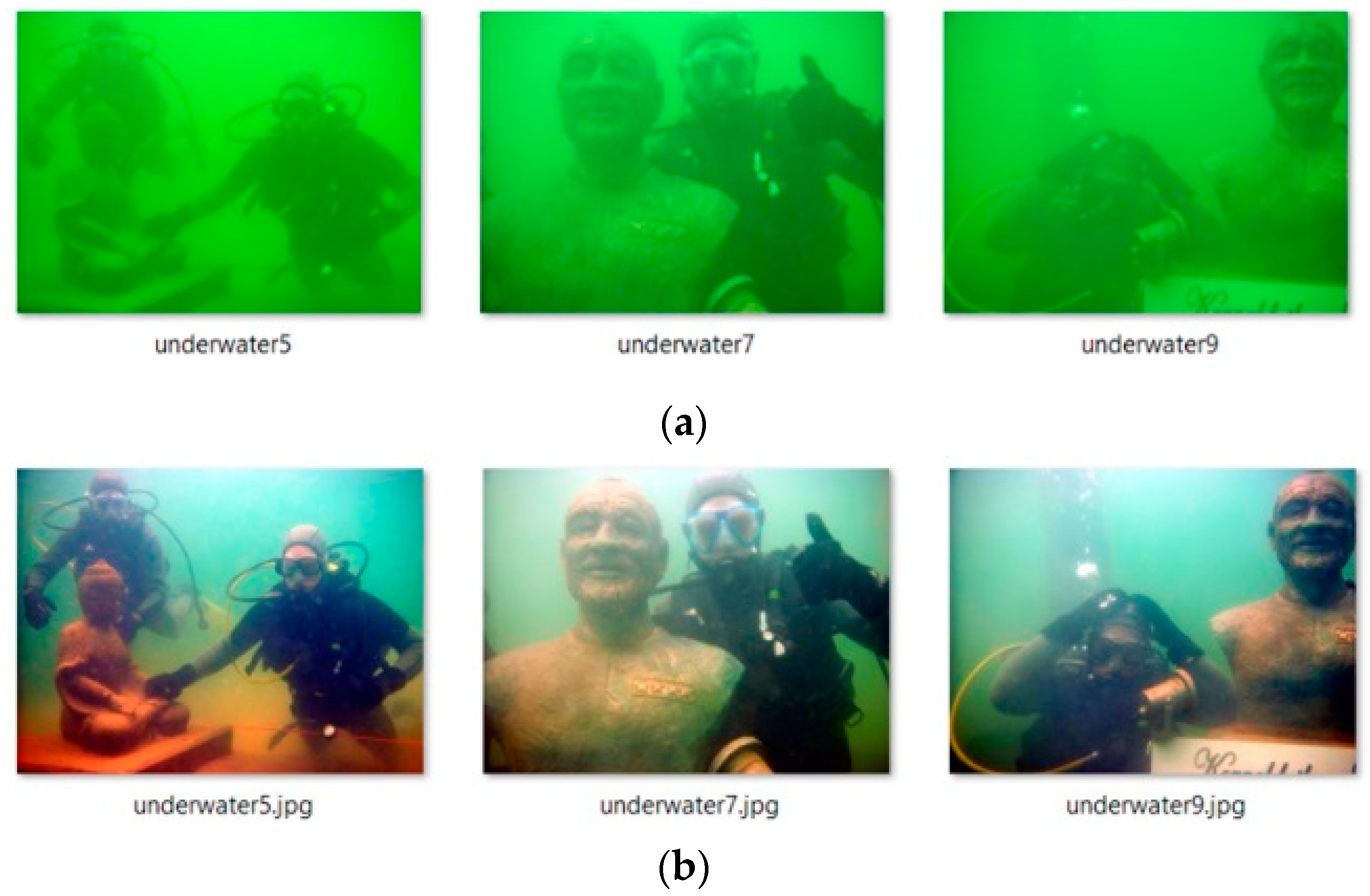
4.1. Underwater Images

4.1.1. Subjective Evaluation

Even though objective metrics have been used for underwater image enhancement and restoration evaluation, they were initially developed for images acquired on land. Thus, some measures have been developed for subjective evaluation of underwater images. These include the Underwater Color Image Quality Evaluation (UCIQE) metric proposed by Yang and Sowmya [82] and the underwater image quality metric (UIQM) [83]. However, the colorfulness parameter, which is utilized in this scenario, is incorporated into the UCIQE metric. The colorfulness and the color enhancement factor have high correlations with the subjective, human-based mean opinion score (MOS) [81]. Additionally, according to Reference [82], “CIELAB color space-based subjective evaluation indicates that sharpness and colorful factors are highly correlated with the subjective image quality perception.” Additionally, they note that “subjective quality metrics give the most reliable outcomes but are expensive, time-consuming, and impractical for real-time implementation and system integration” [82]. These real-time and integration concerns are the very objectives of the realization of the proposed algorithm.

As noted by El Khoury et al. [84], no single algorithm can yield the best or worst performance for all images. In addition, they state that color and sharpness are always utilized in de-hazing evaluation. Thus, the use of colorfulness, gradient, and sharpness measures are justified. More than 50 underwater images from the literature and the Internet were used in the experiment. Some duplications were permitted due to the varying resolutions and formats of some images since this is another challenge of underwater image evaluation. The images used are shown in Figure 3a while the enhanced images are shown in Figure 3b. The original images were obtained from the website: https://github.com/IsaacChanghau/ImageEnhanceViaFusion [85].

The high-boost filter configuration results in brighter images as opposed to using the high-pass filter configuration (HBFC). However, the contrast and edge enhancement using the high-boost filter version (HPFC) is slightly less when compared to the high-pass filter version. The global contrast operator was unmodified for all experiments. The PA performs well for a majority of the images except for images with non-overlapping color channel histograms.

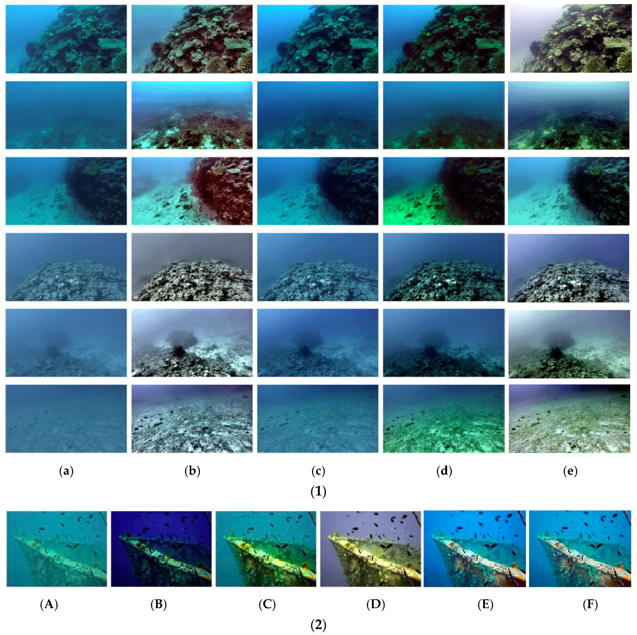
4.1.2. Comparison with Other Algorithms

In Figure 4, we use visual results from Reference [86], which is appended with the visual results of PA using both HPFC and HBFC versions. For the video frames in Figure 4(1) from Reference [86], PA yields the sharpest detail, contrast enhancement, and color correction with the least color distortion when compared to the other methods apart from the method by Ancuti et al. [87] unlike Li et al. [88]. In Figure 4(2), PA yields the sharpest and best color corrected image when compared to results obtained by Emberton et al. [86,89] and Drews-Jr et al. [90]. This is verified in terms of the colorfulness metric used to compute the CEF, which closely correlates with the mean opinion score (MOS) based on the human subjective evaluation [81].

In Table 1, we verify the quality of the results of PA compared with the other algorithms using CEF, UCIQE, and UIQM. The bolded values indicate best results in all tables. The table shows that PA has the most consistent and highest values for the previously mentioned metrics. In Emberton et al. [86], it was claimed that the standard deviation of chroma, σ_c, correlates well with subjective evaluation. Thus, we replicate the table from Reference [86] and only select the σ_c and UCIQE values, which are also computed for the results obtained with PA. The results are shown in Table 1a. The contrast of the luminance (not shown) is consistently highest for PA even though it is not correlated with subjective evaluation and was omitted. Once more, PA yields the most consistent high scores for both metrics.

In Table 1b, PA yields the most colorful and enhanced image, which is shown by the CEF, UIQM, and UCIQE values. Though PA is not optimized as previous or contemporary methods, it is easily the fastest algorithm among the available implementations with acceptable visual outcomes. Furthermore, its multiple applications (alluded to in previous work) and real-time amenability compensates for its minimal impact on the underwater images with non-overlapping histograms. Furthermore, additional experiments showed that the HBFC and HPFC configurations work differently for various images. The percentiles of the global contrast enhancement function are fixed for all experiments to maintain consistency. Only the fractional order and gain are used to switch from HBFC to HPFC. However, the fractional order is kept constant to also maintain consistency. Thus, only the filter gain is the tuning parameter to switch between the two filter configurations.

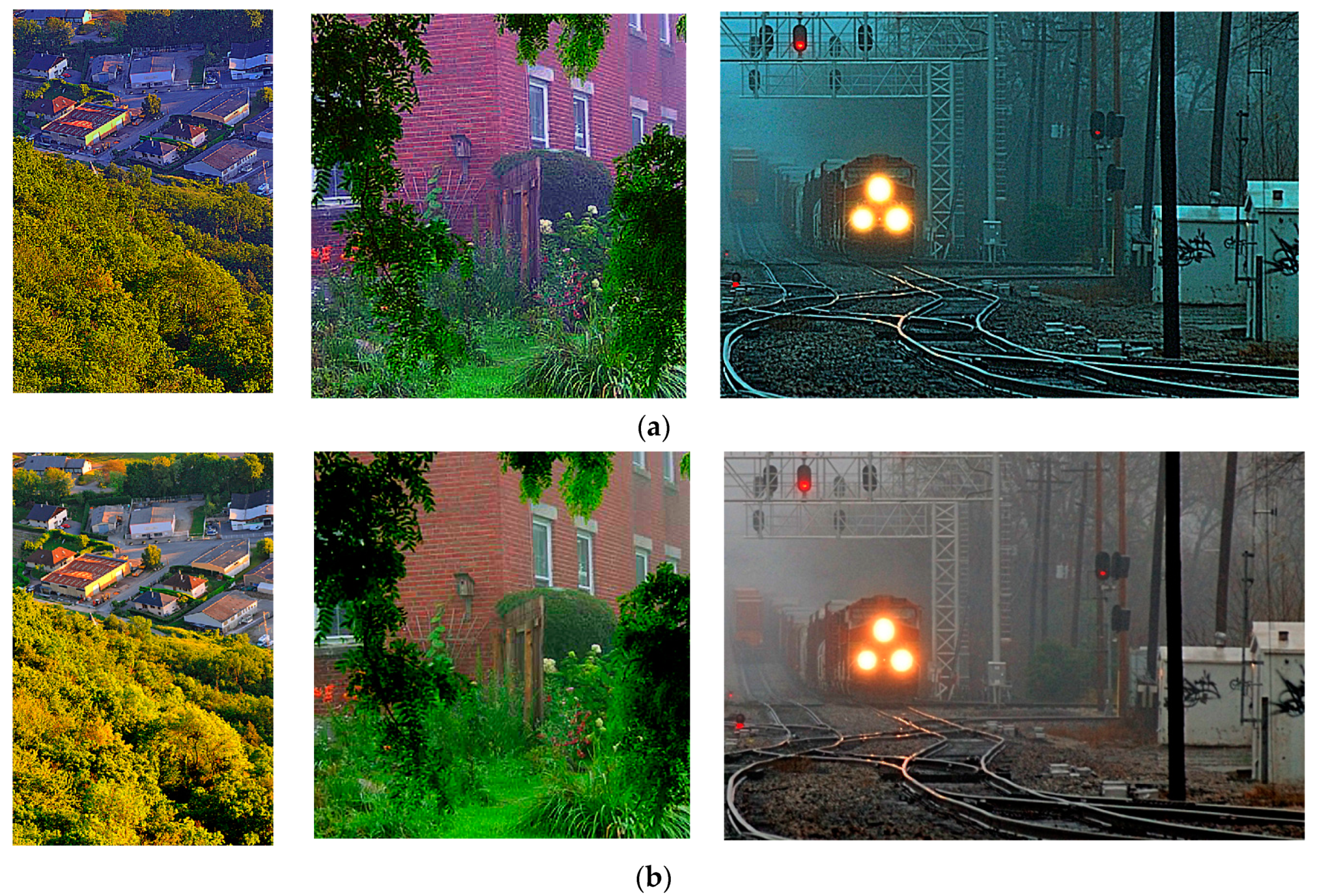
4.2. Hazy Image Enhancement Results

We compare PA against available de-hazing implementations with respective parameters, which is stated by the authors in their papers [53].

• DCP (standard and fast versions) by He, et al. [32]: constant coefficient, $\omega =0.95$, patch size, Ω = 15, regularization parameter, $\lambda =0.0001$ (standard version) and radius of guided filter, r = 24 (fast version).
• Color Attenuation Prior (CAP) by Zhu, et al. [91]: scattering coefficient, $\beta =0.95$ or 1; linear coefficients: ${\theta }_0=0.1893,{\theta }_1=1.0267,{\theta }_2=-1.2966$; transmission lower and upper bounds: $t_0=0.05$, $t_1=1$, regularization parameter, $\epsilon =0.001$.
• Multi-Scale Convolutional Neural Network by Ren et al. [46]: $\gamma =1.3$ for canyon image and $0.8\le \gamma \le 1.5$ for other images.
• Artificial Multi-Exposure-based Fusion (AMEF) by Galdran [54]: clip limit value, c as specified.
• PDE-Retinex set to the default parameters for minimal run-time: $\Delta t=0.25$, $k_{sat}=1.5$.
• PDE-IRCES set to the default parameters for minimal run-time: $\Delta t=0.25$.

The original method by He et al. took about a minimum of 30 s on the current platform for small images. Thus, we focused on the fast version using guided filters. We also present results and comparisons for hazy image contrast enhancement with algorithms from the literature using 53 real benchmark images employed in de-hazing experiments. In addition, the FRIDA3 dataset [92,93] consisting of left and right views of 66 synthetic images was also tested. The algorithms include Tarel and Hautiere [94], Dai et al. [95], Nishino et al. [96], He et al. [32], Galdran et al. [41], Wang and He [97], Zhu et al. [91], Ren et al. [46], Ju et al. [98], partial differential equation-based single scale Retinex GOC-CLAHE (PDE-GOC-SSR-CLAHE or PDE-Retinex) [52], PDE-IRCES [53], and PA. All test images (apart from FRIDA3) used were obtained from the University of Texas at Austin Laboratory for Image & Video Engineering (LIVE) dataset, which can be downloaded from the website: http://live.ece.utexas.edu/research/fog/fade_defade.html) [78]. More detailed and extensive results can be found in additional material [99,100].

Additionally, we present the numerical results for the available algorithm implementations compared with PA in

Table 2. RAG, ratio of visible edges, and saturation parameter values for images processed with He et al. [32], Zhu et al. [90], Ren et al., PDE-GOC-SSR-CLAHE [52], PDE-IRCES [53], and PA.

	Algos	He, et al. [32]	Zhu, et al. [91]	Ren et al. [46]	PDE-GOC-SSR-CLAHE [52]	PDE-IRCES [53]	PA
Images		(Ω = 0.95, w = 15, A = 240, r = 24)	β = 0.95,1; θ0 = 0.1893; θ1 = 1.0267; θ2 = −1.2966; Guided filter: 𝑟 = 60; 𝑡0 = 0.05; 𝑡1 = 1; 𝜀 = 0.001	𝛾 = 1.3 (canyon image) 0.8 ≤ 𝛾 ≤ 1.5 (others)	Δ𝑡 = 0.25; 𝑘𝑠𝑎𝑡 = 1.5	Δ𝑡 = 0.25
Tiananmen		1.8455 /0.9606 /0.1879	1.1866 /1.0041 /0.0814	1.5649 /0.8734 /0.1288	2.8225 /1.0386 /0.0625	2.3219 /1.1614 /0	4.4410 /1.4514 /0.1688
Cones		1.4977 /1.1478 /0.3878	0.9704 /1.0873 /0.2499	1.3818 /1.1042 /0.2956	2.7516 /1.1999 /0.2733	2.5881 /1.2064 /0	4.9702 /1.4620 /0.3142
City1		1.1914 /1.0332 /0.1336	0.9303 /1.0075 /0.2002	1.2989 /1.0232 /0.2002	1.7762 /1.1164 /0.0562	2.4080 /1.3458 /0.00375	3.8282 /1.4898 /0.1712
Canyon		1.7481 /1.1057 /0.3796	1.2880 /1.0679 /0.2412	1.4564 /1.0319 /0.0446	2.5408 /1.2070 /0.3103	2.5224 /1.19684 /0.00019	3.9892 /1.7903 /0.2412
Canon		3.2903 /1.0857 /0.3947	1.7127 /0.9089 /0.3198	2.6871 /1.0832 /0.3831	2.8059 /1.1188 /0.3947	2.8783 /1.3450 /0.00004	8.0224 /1.5785 /0.3942
Mountain		1.7105 /0.9348 /0.0787	1.2092 /0.9307 /0.0984	1.6005 /0.9784 /0.0074	2.7275 /1.0202 /0.0074	2.9827 /1.2977 /0.00007	6.5399 /1.5503 /0.0244
Brick House		1.2006 /0.9747 /0.1172	0.8597 /1.1395 /0.0730	1.2118 /1.0030 /0.1288	1.0836 /1.1135 /0.1021	1.4105 /1.2789 /0	3.0014 /1.3563 /0.0983
Pumpkins		1.5927 /0.9501 /0.1581	0.9311 /0.6726 /0.1333	1.4753 /0.9511 /0.1764	2.4539 /1.0361 /0.1516	2.2777 /1.1626 /0.0001	3.3553 /1.6469 /0.2329
Train		1.5206 /1.0090 /0.1664	0.9797 /1.0509 /0.3265	1.2036 /1.0203 /0.2412	1.5190 /1.1106 /0.3005	2.2569 /1.3589 /0.0038	4.3014 /1.5151 /0.2594
Toys		2.2566 /0.9712 /0.3840	1.6711 /1.0117 /0.2865	2.1568 /0.9576 /0.2827	2.9813 /1.1095 /0.3379	2.1367 /1.2887 /0.00002	4.2837 /1.5937 /0.3736

. The bolded values indicate the best results.

Results indicate that RAG and the ratio of visible edge values are the highest for PA, which was followed by PDE-GOC-SSR-CLAHE, He et al., and Ren et al. Thus, these two metrics indicate maximum edge enhancement corresponding to increased visibility and haze removal. The value of the Canon image yields the highest RAG value and the image result (not shown) depicted a drastic edge and detail enhancement.

The PA can also be configured to process only the intensity channel for hazy images using the HSI and HSV color spaces to avoid hue distortion. However, the algorithm was initially conceived in the RGB space to enable the processing of both underwater and hazy color images without a need for modification. We also present the runtimes of PA in comparison with the other approaches in

Table 3. Runtimes for hazy images processed with He et al. [32], Zhu et al. [91], Ren et al., AMEF, PDE-GOC-SSR-CLAHE [52], PDE-IRCES [53], and PA.

	Algos	He et al. [32]	Zhu et al. [91]	Ren et al. [46]	AMEF [54]	PDE-GOC-SSR-CLAHE [52]	PDE-IRCES [53]	PA
Images
Tiananmen (450 × 600)		1.253494	0.991586	2.362754	1.4088	3.530989	2.330879	0.480659
Cones (384 × 465)		0.850155	0.661314	1.651447	1.0506	2.381621	1.555098	0.268909
City1 (600 × 400)		1.094910	0.875287	2.070620	1.2709	3.203117	2.183417	0.283372
Canyon (600 × 450)		1.237655	0.972741	2.529734	1.5066	3.821395	2.306129	0.309343
Canon (525 × 600)		1.431257	1.135376	2.890541	1.6958	4.187972	2.717652	0.374638
Mountain (400 × 600)		1.129231	0.880835	2.358143	1.2985	3.158335	2.055685	0.360240
Brick house (711 × 693)		2.230871	1.667610	5.234674	2.3618	6.395965	4.385789	1.102332
Pumpkins (400 × 600)		1.125475	0.901815	2.253179	1.5018	3.152969	2.143529	0.407310
Train (400 × 600)		1.105757	0.849072	2.075004	1.2935	3.178277	1.995436	0.365481
Toys (360 × 500)		0.844945	0.657376	1.578068	1.0387	2.429651	1.545031	0.260878

and Figure 5 to further showcase the low computational complexity of the algorithm. The bolded values indicate the best results. Only the method by Ren et al. is fully optimized for GPU computation with PA and other algorithms using parallel computation where possible. Results indicate that PA is the fastest algorithm of all the compared ones. Furthermore, the revised formulation combined with the RGB-IV does not increase run-time considerably except for images with very large dimensions. Nevertheless, the run-time is still much less than the algorithms by He et al., Zhu et al., and Ren et al. The revised scheme is also much easier to implement in digital hardware than the earlier version due to spatial filter structures.

5. Visual Comparison of AMEF and PA and Discussion

The key components of the enhancement capability of AMEF are the CLAHE and Gamma Correction (GC) algorithm. Unlike the PDE-GOC-CLAHE, which included the CLAHE and minimized its negative effects [52], the AMEF does not possess such features. We directly compare and present a sample of visual results of the state-of-the-art AMEF with PA in Figure 6, Figure 7, Figure 8 and Figure 9. Based on visual observation, AMEF generally yields poor results without constant tuning of the clip limit, Figure 6c shows that PA can replicate the results of the AMEF by utilizing a high-boost filter with slightly better contrast than AMEF without CLAHE. Adding CLAHE to PA yields better results than AMEF with CLAHE.

The AMEF de-hazing algorithm yields images with halos and color distortion similar to or worse than the CLAHE-based or Retinex-based de-hazing algorithms, which is seen in the Brick house image in Figure 7b. The AMEF is mainly suited to images with thick haze as seen in the Train image in Figure 7b even though there is color fading. The Horses image was processed using c = 0.03 for AMEF and PA was processed using both filter settings, which is shown in Figure 8. This is one of the images where AMEF performs adequately even though any slight increase in c leads to heavy color distortion. Increasing the clip limit of the CLAHE in the AMEF leads to increased color distortion.

Additionally, the AMEF algorithm is neither optimized nor adaptive and requires constant tuning of this clip limit parameter to obtain the best results for each hazy image. This makes the AMEF algorithm impractical for effective batch (or real-time image de-hazing) processing since these issues were consistently observed using several benchmark hazy images. Ultimately, PA is much faster than the AMEF algorithm while yielding good enhancement results without halos, color degradation, or the need to constantly adjust parameters. Additionally, the AMEF is unable to enhance underwater images while PA effortlessly performs this operation, which is seen in Figure 9.

6. Conclusions

A fast, adaptive, and versatile multi-scale, fractional order-based hazy and underwater image enhancement algorithm with a relatively simplified structure suitable for hardware implementation has been proposed and developed. The earlier problems of the algorithm were addressed by automated balanced weighting of the filtered images used in the fusion process. The adherence to image entropy and standard deviation features coupled with global and local contrast enhancement ensures that visibility is greatly improved in the final result. Furthermore, comparisons with a recent state-of-the-art, multi-scale algorithm shows that the proposed approach is unmatched in several aspects such as speed, consistency, versatility, adaptability, and flexibility. Results show that the proposed scheme achieves the stated objectives and can be easily realized in hardware systems for fast image processing in challenging imaging environments.

References

1. Lee, S.; Yun, S.; Nam, J.H.; Won, C.S.; Jung, S.W. A review on dark channel prior based image dehazing algorithms. EURASIP J. Image Video Process. 2016, 2016, 1–23. [Google Scholar] [CrossRef]
2. Schettini, R.; Corchs, S. Underwater Image Processing: State of the Art of Smoothing and Image Enhancement Methods. EURASIP J. Adv. Signal Process. 2010, 2010, 1–14. [Google Scholar] [CrossRef]
3. Gibson, K.; Nguyen, T. Fast single image fog removal using the adaptive Wiener Filter. In Proceedings of the 2013 20th IEEE International Conference on Image Processing (ICIP), Melbourne, Australia, 15–18 September 2013. [Google Scholar]
4. Galdran, A.; Pardo, D.; Picón, A.; Alvarez-Gila, A. Automatic red-channel underwater image restoration. J. Vis. Commun. Image R. 2015, 26, 132–145. [Google Scholar] [CrossRef]
5. Li, C.; Guo, J.; Wang, B.; Cong, R.; Zhang, Y.; Wang, J. Single underwater image enhancement based on color cast removal and visibility restoration. J. Electron. Imaging 2016, 25, 1–15. [Google Scholar] [CrossRef]
6. Li, C.; Guo, J. Underwater image enhancement by dehazing and color correction. SPIE J. Electron. Imaging 2015, 24, 033023. [Google Scholar] [CrossRef]
7. Zhao, X.; Jin, T.; Qu, S. Deriving inherent optical properties from background color and underwater image enhancement. Ocean Eng. 2015, 94, 163–172. [Google Scholar] [CrossRef]
8. Chiang, J.; Chen, Y. Underwater image enhancement by wavelength compensation and dehazing. IEEE Trans. Image Process. 2012, 21, 1756–1769. [Google Scholar] [CrossRef] [PubMed]
9. Wen, H.; Tian, Y.; Huang, T.; Gao, W. Single underwater image enhancement with a new optical model. In Proceedings of the IEEE International Symposium on Conference on Circuits and Systems (ISCAS), Beijing, China, 19–23 May 2013. [Google Scholar]
10. Serikawa, S.; Lu, H. Underwater image dehazing using joint trilateral filter. Comput. Electr. Eng. 2014, 40, 41–50. [Google Scholar] [CrossRef]
11. Carlevaris-Bianco, N.; Mohan, A.; Eustice, R.M. Initial results in underwater single image dehazing. In Proceedings of the IEEE International Conference on Oceans, Seattle, WA, USA, 20–23 September 2010. [Google Scholar]
12. Chiang, J.Y.; Chen, Y.C.; Chen, Y.F. Underwater Image Enhancement: Using Wavelength Compensation and Image Dehazing (WCID). In International Conference on Advanced Concepts for Intelligent Vision Systems; Springer: Berlin/Heidelberg, Germany; Ghent, Belgium, 22–25 August 2011; pp. 372–383. [Google Scholar]
13. Iqbal, K.; Salam, R.A.; Osman, A.; Talib, A.Z. Underwater image enhancement using an integrated color model. IAENG Int. J. Comput. Sci. 2007, 34, 529–534. [Google Scholar]
14. Ghani, A.S.A.; Isa, N.A.M. Underwater image quality enhancement through integrated color model with Rayleigh distribution. Appl. Soft Comput. 2015, 27, 219–230. [Google Scholar] [CrossRef]
15. Fu, X.; Zhuang, P.; Huang, Y.; Liao, Y.; Zhang, X.P.; Ding, X. A retinex-based enhancing approach for single underwater image. In Proceedings of the International Conference on Image Processing (ICIP), Paris, France, 27–30 October 2014. [Google Scholar]
16. Gouinaud, H.; Gavet, Y.; Debayle, J.; Pinoli, J.C. Color Correction in the Framework of Color Logarithmic Image Processing. In Proceedings of the IEEE 7th International Symposium on Image and Signal Processing and Analysis (ISPA), Dubrovnik, Croatia, 4–6 September 2011. [Google Scholar]
17. Bazeille, S.; Quidu, I.; Jaulin, L.; Malkasse, J.P. Automatic underwater image pre-processing. In Proceedings of the Characterisation du Milieu Marin, CMM, Brest, France, 16–19 October 2006. [Google Scholar]
18. Chambah, M.; Semani, D.; Renouf, A.; Coutellemont, P.; Rizzi, A. Underwater Color Constancy: Enhancement of Automatic Live Fish Recognition. In Proceedings of the 16th Annual symposium on Electronic Imaging, San Jose, CA, USA, 18–22 January 2004. [Google Scholar]
19. Torres-Mendez, L.A.; Dudek, G. Color correction of underwater images for aquatic robot inspection. In Proceedings of the 5th International Workshop on Energy Minimization Methods in Computer Vision and Pattern Recognition (EMMCVPR ‘05), Saint Augustine, FL, USA, 9–11 November 2005. [Google Scholar]
20. Ahlen, J.; Sundgren, D.; Bengtsson, E. Application of underwater hyperspectral data for color correction purposes. Pattern Recognit. Image Anal. 2007, 17, 170–173. [Google Scholar] [CrossRef]
21. Ahlen, J. Colour Correction of Underwater Images Using Spectral Data. Ph.D. Thesis, Uppsala University, Uppsala, Sweden, 2005. [Google Scholar]
22. Petit, F.; Capelle-Laizé, A.S.; Carré, P. Underwater image enhancement by attenuation inversion with quaternions. In Proceedings of the IEEE International Conference on Acoustics, Speech and Signal Processing (ICASSP), Taipei, Taiwan, 19–24 April 2009. [Google Scholar]
23. Bianco, G.; Muzzupappa, M.; Bruno, F.; Garcia, R.; Neumann, L. A New Colour Correction Method For Underwater Imaging. In Proceedings of the International Archives of the Photogrammetry, Remote Sensing and Spatial Information Science, Piano di Sorrento, Italy, 16 April 2015. [Google Scholar]
24. Prabhakar, C.; Praveen, P.K. An Image Based Technique for Enhancement of Underwater Images. Int. J. Mach. Intel. 2011, 3, 217–224. [Google Scholar]
25. Lu, H.; Li, Y.; Zhang, L.; Serikawa, S. Contrast enhancement for images in turbid water. J. Opt. Soc. Am. 2015, 32, 886–893. [Google Scholar] [CrossRef] [PubMed]
26. Nnolim, U.A. Smoothing and enhancement algorithms for underwater images based on partial differential equations. SPIE J. Electron. Imaging 2017, 26, 1–21. [Google Scholar] [CrossRef]
27. Nnolim, U.A. Improved partial differential equation (PDE)-based enhancement for underwater images using local-global contrast operators and fuzzy homomorphic processes. IET Image Process. 2017, 11, 1059–1067. [Google Scholar] [CrossRef]
28. Garcia, R.; Nicosevici, T.; Cufi, X. On the way to solve lighting problems in underwater imaging. In Proceedings of the IEEE Oceans Conference Record, Biloxi, MI, USA, 29–31 October 2002. [Google Scholar]
29. Rzhanov, Y.; Linnett, L.M.; Forbes, R. Underwater video mosaicing for seabed mapping. In Proceedings of the IEEE International Conference on Image Processing, Vancouver, BC, Canada, 10–13 September 2000. [Google Scholar]
30. Singh, H.; Howland, J.; Yoerger, D.; Whitcomb, L. Quantitative photomosaicing of underwater imagery. In Proceedings of the IEEE Oceans Conference, Nice, France, 28 September–1 October 1998. [Google Scholar]
31. Fattal, R. Dehazing using Colour Lines. ACM Trans. Graphic. 2009, 28, 1–14. [Google Scholar]
32. He, K.; Sun, J.; Tang, X. Single Image Haze Removal Using Dark Channel Prior. IEEE Trans. Pattern Anal. Mach. Intel. (PAMI) 2010, 33, 2341–2353. [Google Scholar]
33. Fang, S.; Zhan, J.; Cao, Y.; Rao, R. Improved single image dehazing using segmentation. In Proceedings of the 17th IEEE International Conference on Image Processing (ICIP), Hong Kong, China, 26–29 September 2010. [Google Scholar]
34. Cui, T.; Tian, J.; Wang, E.; Tang, Y. Single image dehazing by latent region-segmentation based transmission estimation and weighted L1-norm regularisation. IET Image Process. 2017, 11, 145–154. [Google Scholar] [CrossRef]
35. Senthamilarasu, V.; Baskaran, A.; Kutty, K. A New Approach for Removing Haze from Images. In Proceedings of the International Conference on Image Processing, Computer Vision, and Pattern Recognition (IPCV), Brasov, Romania, 4–16 August 2014. [Google Scholar]
36. Ancuti, C.O.; Ancuti, C.; Bekaert, P. Effective single image dehazing by fusion. In Proceedings of the 17th IEEE International Conference on Image Processing (ICIP), Hong Kong, China, 26–29 September 2010. [Google Scholar]
37. Galdran, A.; Vazquez-Corral, J.; Pardo, D.; Bertalmio, M. Fusion-based Variational Image Dehazing. IEEE Signal Process. Lett. 2017, 24, 151–155. [Google Scholar] [CrossRef]
38. Carr, P.; Hartley, R. Improved Single Image Dehazing using Geometry. In Proceedings of the IEEE Digital Image Computing: Techniques and Applications, Melbourne, Australia, 1 December 2009. [Google Scholar]
39. Park, D.; Han, D.K.; Ko, H. Single image haze removal with WLS-based edge-preserving smoothing filter. In Proceedings of the IEEE International Conference on Acoustics, Speech and Signal Processing (ICASSP), Vancouver, VAN, Canada, 26–31 May 2013. [Google Scholar]
40. Galdran, A.; Vazquez-Corral, J.; Pardo, D.; Bertalmio, M.A. Variational Framework for Single Image Dehazing. In Computer Vision—ECCV 2014 Workshops; Springer: Zurich, Switzerland, 6–12 September 2014. [Google Scholar]
41. Galdran, A.; Vazquez-Corral, J.; Pardo, D.; Bertalmio, M. Enhanced Variational Image Dehazing. SIAM J. Imaging Sci. 2015, 8, 1519–1546. [Google Scholar] [CrossRef] [Green Version]
42. Liu, X.; Zeng, F.; Huang, Z.; Ji, Y. Single color image dehazing based on digital total variation filter with color transfer. In Proceedings of the 20th IEEE International Conference on Image Processing (ICIP), Melbourne, VIC, Australia, 15–18 September 2013. [Google Scholar]
43. Dong, X.M.; Hu, X.Y.; Peng, S.L.; Wang, D.C. Single color image dehazing using sparse priors. In Proceedings of the 17th IEEE International Conference on Image Processing (ICIP), Hong Kong, China, 26–29 September 2010. [Google Scholar]
44. Meng, G.; Wang, Y.; Duan, J.; Xiang, S.; Pan, C. Efficient Image Dehazing with Boundary Constraint and Contextual Regularization. In Proceedings of the IEEE International Conference on Computer Vision (ICCV), Sydney, Australia, 1–8 December 2013. [Google Scholar]
45. Zhang, X.S.; Gao, S.B.; Li, C.Y.; Li, Y.J. A Retina Inspired Model for Enhancing Visibility of Hazy Images. Front. Comput. Sci. 2015, 9, 1–13. [Google Scholar] [CrossRef] [PubMed]
46. Ren, W.; Liu, S.; Zhang, H.; Pan, J.; Cao, X.; Yang, M.H. Single Image Dehazing via Multi-Scale Convolutional Neural Networks. In Proceedings of the European Conference on Computer Vision 2016, Amsterdam, The Netherlands, 8 October 2016. [Google Scholar]
47. Yang, S.; Zhu, Q.; Wang, J.; Wu, D.; Xie, Y. An Improved Single Image Haze Removal Algorithm Based on Dark Channel Prior and Histogram Specification. In Proceedings of the 3rd International Conference on Multimedia Technology (ICMT), Brno, Czech Republic, 22 November 2013. [Google Scholar]
48. Guo, F.; Cai, Z.; Xie, B.; Tang, J. Automatic Image Haze Removal Based on Luminance Component. In Proceedings of the 6th International Conference on Wireless Communications Networking and Mobile Computing (WiCOM), Chengdu, China, 23–25 September 2010. [Google Scholar]
49. Nair, D.; Kumar, P.A.; Sankaran, P. An Effective Surround Filter for Image Dehazing. In Proceedings of the ICONIAAC 14, Amritapuri, India, 10–11 October 2014. [Google Scholar]
50. Xie, B.; Guo, F.; Cai, Z. Improved Single Image Dehazing Using Dark Channel Prior and Multi-scale Retinex. In Proceedings of the International Conference on Intelligent System Design and Engineering Application (ISDEA), Denver, CO, USA, 13–14 October 2010. [Google Scholar]
51. Nnolim, U.A. Sky Detection and Log Illumination Refinement for PDE-Based Hazy Image Contrast Enhancement. 2017. Available online: http://arxiv.org/pdf/1712.09775.pdf (accessed on December 2017).
52. Nnolim, U.A. Partial differential equation-based hazy image contrast enhancement. Comput. Electr. Eng. 2018, in press. [Google Scholar] [CrossRef]
53. Nnolim, U.A. Image de-hazing via gradient optimized adaptive forward-reverse flow-based partial differential equation. J. Circuit. Syst. Comp. 2018, accepted. [Google Scholar] [CrossRef]
54. Galdran, A. Artificial Multiple Exposure Image Dehazing. Signal Process. 2018, 149, 135–147. [Google Scholar] [CrossRef]
55. Zhu, M.; He, B.; Wu, Q. Single Image Dehazing Based on Dark Channel Prior and Energy Minimization. IEEE Signal Process. Lett. 2018, 25, 174–178. [Google Scholar] [CrossRef]
56. Shi, Z.; Zhu, M.; Xia, Z.; Zhao, M. Fast single-image dehazing method based on luminance dark prior. Int. J. Pattern Recognit. 2017, 31, 1754003. [Google Scholar] [CrossRef]
57. Yuan, X.; Ju, M.; Gu, Z.; Wang, S. An Effective and Robust Single Image Dehazing Method Using the Dark Channel Prior. Information 2017, 8, 57. [Google Scholar] [CrossRef]
58. Zhu, Y.; Tang, G.; Zhang, X.; Jiang, J.; Tian, Q. Haze removal method for natural restoration of images with sky. Neurocomputing 2018, 275, 499–510. [Google Scholar] [CrossRef]
59. Wang, X.; Ju, M.; Zhang, D. Automatic hazy image enhancement via haze distribution estimation. Adv. Mech. Eng. 2018, 10, 1687814018769485. [Google Scholar] [CrossRef]
60. Du, Y.; Li, X. Recursive Deep Residual Learning for Single Image Dehazing. In Proceedings of the IEEE Conference on Computer Vision and Pattern Recognition Workshops 2018, Salt Lake City, Utah, 18–22 June 2018. [Google Scholar]
61. Jiang, H.; Lu, N.; Yao, L.; Zhang, X. Single image dehazing for visible remote sensing based on tagged haze thickness maps. Remote Sens. Lett. 2018, 9, 627–635. [Google Scholar] [CrossRef]
62. Ju, M.Y.; Ding, C.; Zhang, D.Y.; Guo, Y.J. Gamma-Correction-Based Visibility Restoration for Single Hazy Images. IEEE Signal Process. Lett. 2018, 25, 1084–1088. [Google Scholar] [CrossRef]
63. Ki, S.; Sim, H.; Choi, J.S.; Seo, S.; Kim, S.; Kim, M. Fully End-to-End learning based Conditional Boundary Equilibrium GAN with Receptive Field Sizes Enlarged for Single Ultra-High Resolution Image Dehazing. In Proceedings of the IEEE Conference on Computer Vision and Pattern Recognition Workshops 2018, Salt Lake City, UT, USA, 18–22 June 2018. [Google Scholar]
64. Li, C.; Guo, J.; Porikli, F.; Fu, H.; Pang, Y. A Cascaded Convolutional Neural Network for Single Image Dehazing. IEEE Access. 2018, 6, 24877–24887. [Google Scholar] [CrossRef]
65. Li, R.; Pan, J.; Li, Z.; Tang, J. Single Image Dehazing via Conditional Generative Adversarial Network. Methods 2018, 3, 24. [Google Scholar]
66. Luan, Z.; Zeng, H.; Shang, Y.; Shao, Z.; Ding, H. Fast Video Dehazing Using Per-Pixel Minimum Adjustment. Math. Probl. Eng. 2018, 2018, 9241629. [Google Scholar] [CrossRef]
67. Mondal, R.; Santra, S.; Chanda, B. Image Dehazing by Joint Estimation of Transmittance and Airlight using Bi-Directional Consistency Loss Minimized FCN. In Proceedings of the IEEE Conference on Computer Vision and Pattern Recognition Workshops 2018, Salt Lake City, UT, USA, 18–22 June 2018. [Google Scholar]
68. Qin, M.; Xie, F.; Li, W.; Shi, Z.; Zhang, H. Dehazing for Multispectral Remote Sensing Images Based on a Convolutional Neural Network with the Residual Architecture. IEEE J. Sel. Top. Appl. Earth Observ. Remote Sens. 2018, 11, 1645–1655. [Google Scholar] [CrossRef]
69. Santra, S.; Mondal, R.; Chanda, B. Learning a Patch Quality Comparator for Single Image Dehazing. IEEE Trans. Image Process. 2018, 27, 4598–4607. [Google Scholar] [CrossRef] [PubMed]
70. Song, Y.; Li, J.; Wang, X.; Chen, X. Single Image Dehazing Using Ranking Convolutional Neural Network. IEEE Trans. Multimedia 2018, 20, 1548–1560. [Google Scholar] [CrossRef]
71. Zhang, H.; Sindagi, V.; Patel, V.M. Multi-scale Single Image Dehazing using Perceptual Pyramid Deep Network. In Proceedings of the IEEE Conference on Computer Vision and Pattern Recognition Workshops 2018, Salt Lake City, UT, USA, 18–22 June 2018. [Google Scholar]
72. Li, J.; Li, G.; Fan, H. Image Dehazing using Residual-based Deep CNN. IEEE Access 2018, 6, 26831–26842. [Google Scholar] [CrossRef]
73. Lu, J.; Li, N.; Zhang, S.; Yu, Z.; Zheng, H.; Zheng, B. Multi-scale adversarial network for underwater image restoration. Opt. Laser Technol. 2018, in press. [Google Scholar] [CrossRef]
74. Yang, Q.; Chen, D.; Zhao, T.; Chen, Y. Fractional calculus in image processing: A review. Fract. Calc. Appl. Anal. 2016, 19, 1222–1249. [Google Scholar] [CrossRef]
75. Patrascu, V. Image enhancement method using piecewise linear transforms. In Proceedings of the European Signal Processing Conference (EUSIPCO-2004), Vienna, Austria, 6–10 September 2004. [Google Scholar]
76. Baliga, A.B. Face Illumination Normalization with Shadow Consideration. Master’s Thesis, Carnegie Mellon University, Pittsburgh, PA, USA, May 2004. [Google Scholar]
77. Nnolim, U.A. An adaptive RGB colour enhancement formulation for Logarithmic Image Processing-based algorithms. Optik 2018, 154, 192–215. [Google Scholar] [CrossRef]
78. Laboratory for Image & Video Engineering (LIVE). Referenceless Prediction of Perceptual Fog Density and Perceptual Image Defogging. Available online: http://live.ece.utexas.edu/research/fog/fade_defade.html (accessed on 30 June 2018).
79. Shen, X.; Li, Q.; Tan, Y.; Shen, L. An Uneven Illumination Correction Algorithm for Optical Remote Sensing Images Covered with Thin Clouds. Remote Sens. 2015, 7, 11848–11862. [Google Scholar] [CrossRef] [Green Version]
80. Matkovic, K.; Neumann, L.; Neumann, A.; Psik, T.; Purgathofer, W. Global Contrast Factor-a New Approach to Image Contrast. In Proceedings of the 1st Eurographics Conference on Computational Aesthetics in Graphics, Visualization and Imaging, Girona, Spain, 18–20 May 2005. [Google Scholar]
81. Susstrunk, S.; Hasler, D. Measuring Colourfulness in Natural Images. In Proceedings of the IS&T/SPIE Electronic Imaging 2003: Human Vision and Electronic Imaging VIII, Santa Clara, California, CA, USA, 21–24 January 2003. [Google Scholar]
82. Yang, M.; Sowmya, A. An Underwater Color Image Quality Evaluation Metric. IEEE Trans. Image Process. 2015, 24, 6062–6071. [Google Scholar] [CrossRef] [PubMed]
83. Panetta, K.; Gao, C.; Agaian, S. Human-visual-system-inspired underwater image quality measures. IEEE J. Ocean Eng. 2016, 41, 541–551. [Google Scholar] [CrossRef]
84. El Khoury, J.; Le Moan, S.; Thomas, J.B.; Mansouri, A. Color and sharpness assessment of single image dehazing. Multimed. Tools Appl. 2018, 77, 15409–15430. [Google Scholar] [CrossRef]
85. Changhau, I. Underwater Image Enhance via Fusion (IsaacChanghau/ImageEnhanceViaFusion). Available online: https://github.com/IsaacChanghau/ImageEnhanceViaFusion (accessed on 30 July 2018).
86. Emberton, S.; Chittka, L.; Cavallaro, A. Underwater image and video dehazing with pure haze region segmentation. Comput. Vis. Image Und. 2018, 168, 145–156. [Google Scholar] [CrossRef] [Green Version]
87. Ancuti, C.; Ancuti, C.; Haber, T.; Bekaert, P. Enhancing underwater images and videos by fusion. In Proceedings of the IEEE Conference on Computer Vision and Pattern Recognition, Providence, Rhode Island, 16 June 2012. [Google Scholar]
88. Li, Z.; Tan, P.; Tan, R.T.; Zou, D.; Zhou, S.Z.; Cheong, L.F. Simultaneous video defogging and stereo reconstruction. In Proceedings of the IEEE Conferene on Computer Vision and Pattern Recognition, Boston, MA, USA, 7–12 June 2015. [Google Scholar]
89. Emberton, S.; Chittka, L.; Cavallaro, A. Hierarchical rank-based veiling light estimation for underwater dehazing. In Proceedings of the British Machine Vision Conference, Swansea, UK, 7–10 September 2015. [Google Scholar]
90. Drews-Jr, P.; Nascimento, E.; Moraes, F.; Botelho, S.; Campos, M.; Grande-Brazil, R.; Horizonte-Brazil, B. Transmission estimation in underwater single images. In Proceedings of the IEEE International Conference on Computer Vision Workshop, Sydney, NSW, Australia, 2–8 December 2013. [Google Scholar]
91. Zhu, Q.; Mai, J.; Shao, L.A. Fast Single Image Haze Removal Algorithm Using Color Attenuation Prior. IEEE Trans. Image Process. 2015, 24, 3522–3533. [Google Scholar] [PubMed]
92. Caraffa, L.; Tarel, J.P. Stereo Reconstruction and Contrast Restoration in Daytime Fog. In Proceedings of the 11th IEEE Asian Conference on Computer Vision (ACCV’12), Daejeon, Korea, 5–9 November 2012. [Google Scholar]
93. Tarel, J.P.; Cord, A.; Halmaoui, H.; Gruyer, D.; Hautiere, N. Improved Visibility of Road Scene Images under Heterogeneous Fog. In Proceedings of the IEEE Intelligent Vehicles Symposium (IV’10), San Diego, CA, USA, 21–24 June 2010. [Google Scholar]
94. Tarel, J.; Hautiere, N. Fast visibility restoration from a single color or gray level image. In Proceedings of the IEEE 12th International Conference on Computer Vision, Kyoto, Japan, 29 September–2 October 2009. [Google Scholar]
95. Dai, S.K.; Tarel, J.P. Adaptive Sky Detection and Preservation in Dehazing Algorithm. In Proceedings of the IEEE International Symposium on Intelligent Signal Processing and Communication Systems (ISPACS), Nusa Dua, Bali, Indonesia, 9–12 November 2015. [Google Scholar]
96. Nishino, K.; Kratz, L.; Lombardi, S. Bayesian Defogging. Int. J. Comput. Vis. 2012, 98, 263–278. [Google Scholar] [CrossRef]
97. Wang, W.; He, C. Depth and Reflection Total Variation for Single Image Dehazing. arXiv 2016, arXiv:1601.05994. [Google Scholar]
98. Ju, M.; Zhang, D.; Wang, X. Single image dehazing via an improved atmospheric scattering model. Vis. Comput. 2017, 33, 1613–1625. [Google Scholar] [CrossRef]
99. Nnolim, U.A. Adaptive multi-scale entropy fusion de-hazing based on fractional order. Preprints 2018. [Google Scholar] [CrossRef]
100. Nnolim, U.A. Fractional Multiscale Fusion-based De-hazing. Available online: https://arxiv.org/abs/1808.09697 (accessed on 29 August 2018).
Figure 1. Proposed algorithm (PA) for enhancing hazy and underwater images.
Jimaging 04 00108 g001
Figure 2. Processed images using (a) previous configuration (b) improved configuration of PA.
Jimaging 04 00108 g002
Figure 3. (a) Original underwater images processed with (b) PA (Source images obtained from [85]).
Jimaging 04 00108 g003
Figure 4. (1) Image results from Reference [86] (http://dx.doi.org/10.1016/j.cviu.2017.08.003; http://creativecommons.org/licenses/by/4.0/) amended with visual results of PA: (a) Original first video frames of sequences S1 to S6 (b) Ancuti et al. [87], (c) Li et al. [88], and (d) Emberton et al. [86]. (e) PA (HBFC) (f) PA (HPFC). (2) (A) Original image [4] processed with algorithms proposed by (B) Drews-jr et al. [90], (C) Emberton et al. [89], (D) Emberton et al. [86], (E) PA (HBFC), and (F) PA (HPF.C).
Jimaging 04 00108 g004
Figure 5. Runtime comparison of various algorithms using (a) 53 real and 66 synthetic (b) left and (c) right view hazy images.
Jimaging 04 00108 g005
Figure 6. (a) PA, (b) without GOCS, (c) using high-boost filter setting, (d) AMEF (c = 0.1), (e) AMEF (c = 0.01), and (f) AMEF without CLAHE.
Jimaging 04 00108 g006
Figure 7. (a) PA (high-boost) (b,c) PA (d) AMEF (c = 0.03) (e,f) AMEF (c = 0.1).
Jimaging 04 00108 g007
Figure 8. (a) PA, (b) with high-boost filter setting, (c) AMEF (c = 0.03), and (d) AMEF without CLAHE.
Jimaging 04 00108 g008
Figure 9. (a) Original underwater image processed with (b) AMEF (c = 0.1) (c,d) PA.
Jimaging 04 00108 g009