
Efficient Retrieval of Images with Irregular Patterns Using Morphological Image Analysis: Applications to Industrial and Healthcare Datasets


Abstract
:1. Introduction
- A novel ImR framework that uses the morphological features to retrieve images containing irregular patterns.
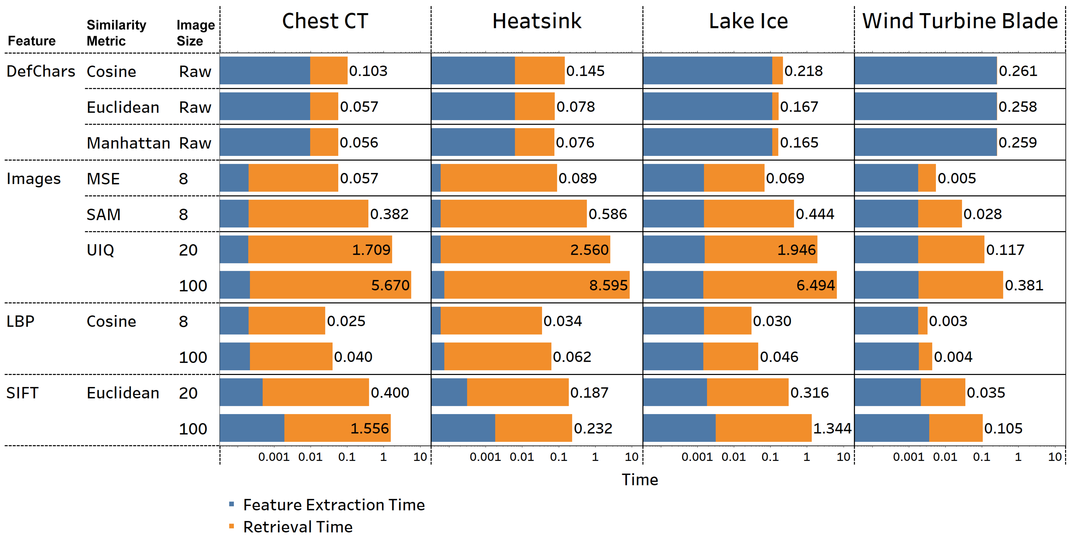
- Retrieval and time performance comparison of the proposed ImR framework using different features (i.e., the DefChars, LBP, SIFT, and resized images) across various datasets.
- An empirical comparison of the retrieval and time performance between the proposed ImR framework and a state-of-the-art DL-based ImR approach.
2. Related Works
2.1. Feature Extraction and Relevant Similarity Metrics for Retrieving Images
2.2. Recent Works to Retrieve Industrial and Healthcare Images with Irregular Patterns
3. Proposed Image Retrieval Framework
3.1. Repository Process
3.2. Retrieval Process
4. Experiment Methodology
4.1. Datasets
- The wind turbine blade dataset, provided by our industrial partner Railston & Co., Ltd., Nottingham, United Kingdom, contains 191 images with 304 irregular patterns across four classes (crack, void, erosion, and other). The images of wind turbine blade defects were captured during inspection; mask annotations were gathered from Zhang et al.’s experiment [31].
- The chest CT dataset was collected from Ter-Sarkisov’s [32] experiment and utilised to detect and classify the COVID-19 infection regions shown in chest CT scans. The chest CT dataset contains 750 images with 4665 irregular patterns across three classes (lung area, ground glass opacity, and consolidation), and the mask annotations were also provided in the dataset.
- The heatsink dataset was collected from Yang et al.’s experiment [33] and used to detect defects on the surfaces of gold-plated tungsten–copper alloy heatsinks. The heatsink dataset contains 1000 images, captured by an industrial camera, with 7007 irregular patterns and corresponding mask annotations across two classes (scratch and stain).
- The Photi-LakeIce (lake ice) dataset was collected from Prabha et al.’s [34] project and utilised to monitor the ice and snow on lakes by using AI techniques. The lake ice dataset contains 4017 images, captured by fixed-position webcams, with 5365 irregular patterns and corresponding mask annotations [34] across four classes (water, ice, snow, and clutter).
4.2. Feature Extraction Method for Image Retrieval
4.3. Similarity Metrics for Image Retrieval
4.3.1. Image-Based Similarity Metrics
4.3.2. Feature-Based Similarity Metrics
4.4. Methodology
- In the initial step (DefChar extraction module) of the experiment, feature sets are extracted:Feature set 1 contains the raw images that have been compressed into four different sizes (i.e., , , , ) with the dual goals of normalisation and acceleration of the retrieval process. Hence, feature set 1 has four subsets of features each corresponding to a different size.Feature set 2 contains DefChars extracted from raw images. Raw images should be utilised when extracting DefChars, due to information loss caused by image resizing.Feature sets 3 and 4 contain LBP and SIFT features extracted from each of the feature subsets described in feature set 1. The parameters of LBP were set to radius = 1, sample points = 8, and method = uniform, following the recommendations by Rahillda et al. [82] based on their experimental results. The SIFT parameters used in this experiment were set according to the guidelines by Lowe [80]: nFeatures = max, nOctaveLayers = 3, contrastThreshold = 0.3, edgeThreshold = 10, and sigma = 1.6. The feature sets are separately stored (indexing module) in a datastore.
- In the next step (similarity computation module), the similarity between a query image and images—represented as feature vectors—found in the datastore is computed. In this experiment, each image from the datasets is iteratively selected to be a query. To compute the similarity between images, feature- and image-based similarity metrics are applied. Feature-based similarity metrics (i.e., Euclidean, cosine, Manhattan, and Jaccard) are utilised for DefChar, SIFT, and LBP features; and image-based similarity metrics (i.e., MSE, SAM, and UIQ) are utilised for compressed raw images.
- Then, the retrieved irregular patterns are ranked (ranking module) according to the computed similarity values. The metrics described in Section 4.5 are applied to evaluate the retrieval performance.
4.5. Evaluation Measures
5. Results and Discussion
- DefChar-based methods refer to the proposed ImR framework using DefChars within the DefChar extraction module.
- Image-based methods refer to the proposed ImR framework using resized images instead of the DefChar extraction module.
- LBP-based methods refer to the proposed ImR framework using LBP features instead of the DefChar extraction module.
- SIFT-based methods refer to the proposed ImR framework using SIFT features instead of the DefChar extraction module.
5.1. Image Retrieval Performance When Using Different Feature Sets and Similarity Metrics across Datasets
5.1.1. Chest CT Dataset
5.1.2. Heatsink Dataset
5.1.3. Lake Ice Dataset
5.1.4. Wind Turbine Blade Dataset
5.2. Overall Performance Comparisons for Image Retrieval Tasks
5.3. Image Retrieval Performance Comparisons between the Proposed ImR Framework and a DL-Based ImR Framework
6. Conclusions and Future Work
Author Contributions
Funding
Institutional Review Board Statement
Informed Consent Statement
Data Availability Statement
Acknowledgments
Conflicts of Interest
Abbreviations
| ImR | Image Retrieval |
| AI | Artificial Intelligence |
| CBIR | Content-based Image Retrieval |
| CNN | Convolutional Neural Network |
| DL | Deep Learning |
| Mean Average Precision | |
| Average Precision | |
| LBP | Local Binary Pattern |
| DefChars | Defect Characteristics |
| SIFT | Scale-Invariant Feature Transform |
| MSE | Mean Squared Error |
| SAM | Spectral Angle Mapper |
| UIQ | Universal Image Quality Index |
| SSIM | Structural Similarity Index |
| CT | Computerised Tomography |
| SG | Super Global |
| Std | Standard Deviation |
Appendix A. ImR Evaluation Results for the Chest CT Dataset

| Feature | Similarity Metric | Image Size | Average | |||||
|---|---|---|---|---|---|---|---|---|
| DefChars | Cosine | Raw | 0.88 ± 0.06 | 0.86 ± 0.06 | 0.85 ± 0.06 | 0.84 ± 0.06 | 0.84 ± 0.06 | 0.85 ± 0.06 |
| DefChars | Euclidean | Raw | 0.88 ± 0.06 | 0.86 ± 0.06 | 0.85 ± 0.06 | 0.84 ± 0.06 | 0.84 ± 0.06 | 0.85 ± 0.06 |
| DefChars | Jaccard | Raw | 0.51 ± 0.19 | 0.49 ± 0.20 | 0.47 ± 0.21 | 0.47 ± 0.21 | 0.47 ± 0.22 | 0.48 ± 0.21 |
| DefChars | Manhattan | Raw | 0.88 ± 0.06 | 0.86 ± 0.07 | 0.85 ± 0.07 | 0.84 ± 0.07 | 0.84 ± 0.07 | 0.85 ± 0.07 |
| Image | MSE | 8 | 0.76 ± 0.22 | 0.74 ± 0.22 | 0.73 ± 0.22 | 0.72 ± 0.22 | 0.71 ± 0.22 | 0.73 ± 0.22 |
| Image | MSE | 20 | 0.75 ± 0.24 | 0.74 ± 0.23 | 0.73 ± 0.23 | 0.72 ± 0.23 | 0.71 ± 0.23 | 0.73 ± 0.23 |
| Image | MSE | 50 | 0.75 ± 0.23 | 0.73 ± 0.23 | 0.73 ± 0.23 | 0.72 ± 0.23 | 0.71 ± 0.23 | 0.73 ± 0.23 |
| Image | MSE | 100 | 0.75 ± 0.23 | 0.73 ± 0.23 | 0.72 ± 0.23 | 0.72 ± 0.23 | 0.71 ± 0.23 | 0.73 ± 0.23 |
| Image | SAM | 8 | 0.72 ± 0.20 | 0.69 ± 0.22 | 0.67 ± 0.22 | 0.66 ± 0.23 | 0.65 ± 0.23 | 0.68 ± 0.22 |
| Image | SAM | 20 | 0.72 ± 0.21 | 0.69 ± 0.22 | 0.67 ± 0.23 | 0.66 ± 0.24 | 0.65 ± 0.24 | 0.68 ± 0.23 |
| Image | SAM | 50 | 0.72 ± 0.21 | 0.69 ± 0.23 | 0.67 ± 0.24 | 0.66 ± 0.24 | 0.65 ± 0.25 | 0.68 ± 0.23 |
| Image | SAM | 100 | 0.72 ± 0.21 | 0.69 ± 0.22 | 0.67 ± 0.24 | 0.66 ± 0.24 | 0.65 ± 0.25 | 0.68 ± 0.23 |
| Image | UIQ | 8 | 0.33 ± 0.58 | 0.33 ± 0.42 | 0.33 ± 0.42 | 0.33 ± 0.31 | 0.33 ± 0.23 | 0.33 ± 0.39 |
| Image | UIQ | 20 | 0.77 ± 0.18 | 0.76 ± 0.17 | 0.75 ± 0.17 | 0.75 ± 0.16 | 0.75 ± 0.16 | 0.76 ± 0.17 |
| Image | UIQ | 50 | 0.77 ± 0.20 | 0.76 ± 0.19 | 0.75 ± 0.19 | 0.75 ± 0.19 | 0.74 ± 0.19 | 0.75 ± 0.19 |
| Image | UIQ | 100 | 0.77 ± 0.21 | 0.76 ± 0.20 | 0.75 ± 0.21 | 0.74 ± 0.21 | 0.74 ± 0.21 | 0.75 ± 0.21 |
| LBP | Cosine | 8 | 0.22 ± 0.16 | 0.22 ± 0.17 | 0.22 ± 0.18 | 0.22 ± 0.18 | 0.23 ± 0.19 | 0.22 ± 0.18 |
| LBP | Cosine | 20 | 0.23 ± 0.28 | 0.21 ± 0.27 | 0.21 ± 0.28 | 0.21 ± 0.28 | 0.21 ± 0.28 | 0.21 ± 0.28 |
| LBP | Cosine | 50 | 0.28 ± 0.28 | 0.29 ± 0.11 | 0.28 ± 0.12 | 0.28 ± 0.08 | 0.28 ± 0.08 | 0.28 ± 0.13 |
| LBP | Cosine | 100 | 0.30 ± 0.24 | 0.30 ± 0.28 | 0.30 ± 0.22 | 0.30 ± 0.19 | 0.31 ± 0.16 | 0.30 ± 0.22 |
| LBP | Euclidean | 8 | 0.22 ± 0.16 | 0.22 ± 0.17 | 0.22 ± 0.18 | 0.22 ± 0.18 | 0.23 ± 0.19 | 0.22 ± 0.18 |
| LBP | Euclidean | 20 | 0.23 ± 0.28 | 0.21 ± 0.27 | 0.21 ± 0.28 | 0.21 ± 0.28 | 0.21 ± 0.28 | 0.21 ± 0.28 |
| LBP | Euclidean | 50 | 0.28 ± 0.28 | 0.29 ± 0.11 | 0.28 ± 0.12 | 0.28 ± 0.08 | 0.28 ± 0.08 | 0.28 ± 0.13 |
| LBP | Euclidean | 100 | 0.30 ± 0.24 | 0.30 ± 0.28 | 0.30 ± 0.22 | 0.30 ± 0.19 | 0.31 ± 0.16 | 0.30 ± 0.22 |
| LBP | Jaccard | 8 | 0.22 ± 0.16 | 0.22 ± 0.17 | 0.22 ± 0.18 | 0.22 ± 0.18 | 0.23 ± 0.19 | 0.22 ± 0.18 |
| LBP | Jaccard | 20 | 0.23 ± 0.28 | 0.21 ± 0.27 | 0.21 ± 0.28 | 0.21 ± 0.28 | 0.21 ± 0.28 | 0.21 ± 0.28 |
| LBP | Jaccard | 50 | 0.28 ± 0.28 | 0.29 ± 0.11 | 0.28 ± 0.12 | 0.28 ± 0.08 | 0.28 ± 0.08 | 0.28 ± 0.13 |
| LBP | Jaccard | 100 | 0.30 ± 0.24 | 0.30 ± 0.28 | 0.30 ± 0.22 | 0.30 ± 0.19 | 0.31 ± 0.16 | 0.30 ± 0.22 |
| LBP | Manhattan | 8 | 0.22 ± 0.16 | 0.22 ± 0.17 | 0.22 ± 0.18 | 0.22 ± 0.18 | 0.23 ± 0.19 | 0.22 ± 0.18 |
| LBP | Manhattan | 20 | 0.23 ± 0.28 | 0.21 ± 0.27 | 0.21 ± 0.28 | 0.21 ± 0.28 | 0.21 ± 0.28 | 0.21 ± 0.28 |
| LBP | Manhattan | 50 | 0.28 ± 0.28 | 0.29 ± 0.11 | 0.28 ± 0.12 | 0.28 ± 0.08 | 0.28 ± 0.08 | 0.28 ± 0.13 |
| LBP | Manhattan | 100 | 0.30 ± 0.24 | 0.30 ± 0.28 | 0.30 ± 0.22 | 0.30 ± 0.19 | 0.31 ± 0.16 | 0.30 ± 0.22 |
| SIFT | Euclidean | 8 | 0.40 ± 0.51 | 0.35 ± 0.41 | 0.35 ± 0.42 | 0.36 ± 0.33 | 0.36 ± 0.26 | 0.36 ± 0.39 |
| SIFT | Euclidean | 20 | 0.56 ± 0.29 | 0.52 ± 0.32 | 0.51 ± 0.33 | 0.51 ± 0.31 | 0.51 ± 0.30 | 0.52 ± 0.31 |
| SIFT | Euclidean | 50 | 0.43 ± 0.40 | 0.44 ± 0.39 | 0.45 ± 0.39 | 0.45 ± 0.39 | 0.44 ± 0.38 | 0.44 ± 0.39 |
| SIFT | Euclidean | 100 | 0.38 ± 0.39 | 0.40 ± 0.35 | 0.42 ± 0.34 | 0.43 ± 0.34 | 0.43 ± 0.33 | 0.41 ± 0.35 |
| Feature | Similarity Metric | Image Size | |||||
|---|---|---|---|---|---|---|---|
| DefChars | Cosine | Raw | 0.93 ± 0.25 | 0.92 ± 0.21 | 0.91 ± 0.21 | 0.90 ± 0.21 | 0.90 ± 0.21 |
| DefChars | Euclidean | Raw | 0.93 ± 0.25 | 0.92 ± 0.21 | 0.91 ± 0.21 | 0.90 ± 0.21 | 0.90 ± 0.21 |
| DefChars | Jaccard | Raw | 0.70 ± 0.46 | 0.69 ± 0.33 | 0.68 ± 0.30 | 0.68 ± 0.29 | 0.68 ± 0.28 |
| DefChars | Manhattan | Raw | 0.94 ± 0.24 | 0.92 ± 0.21 | 0.92 ± 0.20 | 0.91 ± 0.20 | 0.91 ± 0.20 |
| Image | MSE | 8 | 0.93 ± 0.25 | 0.92 ± 0.20 | 0.91 ± 0.20 | 0.90 ± 0.20 | 0.89 ± 0.20 |
| Image | MSE | 20 | 0.94 ± 0.24 | 0.93 ± 0.19 | 0.92 ± 0.19 | 0.91 ± 0.19 | 0.91 ± 0.19 |
| Image | MSE | 50 | 0.94 ± 0.23 | 0.93 ± 0.18 | 0.92 ± 0.18 | 0.92 ± 0.19 | 0.91 ± 0.19 |
| Image | MSE | 100 | 0.94 ± 0.24 | 0.93 ± 0.18 | 0.92 ± 0.18 | 0.92 ± 0.19 | 0.91 ± 0.19 |
| Image | SAM | 8 | 0.94 ± 0.23 | 0.94 ± 0.17 | 0.93 ± 0.16 | 0.92 ± 0.16 | 0.92 ± 0.16 |
| Image | SAM | 20 | 0.96 ± 0.20 | 0.95 ± 0.15 | 0.94 ± 0.15 | 0.93 ± 0.15 | 0.93 ± 0.15 |
| Image | SAM | 50 | 0.96 ± 0.20 | 0.95 ± 0.15 | 0.94 ± 0.15 | 0.94 ± 0.14 | 0.93 ± 0.15 |
| Image | SAM | 100 | 0.96 ± 0.20 | 0.95 ± 0.15 | 0.94 ± 0.15 | 0.94 ± 0.15 | 0.93 ± 0.15 |
| Image | UIQ | 8 | 0.00 ± 0.00 | 0.80 ± 0.00 | 0.80 ± 0.00 | 0.67 ± 0.00 | 0.55 ± 0.00 |
| Image | UIQ | 20 | 0.94 ± 0.23 | 0.92 ± 0.19 | 0.91 ± 0.19 | 0.90 ± 0.19 | 0.89 ± 0.20 |
| Image | UIQ | 50 | 0.95 ± 0.23 | 0.93 ± 0.18 | 0.92 ± 0.18 | 0.91 ± 0.18 | 0.91 ± 0.19 |
| Image | UIQ | 100 | 0.95 ± 0.22 | 0.94 ± 0.17 | 0.93 ± 0.17 | 0.92 ± 0.18 | 0.91 ± 0.18 |
| LBP | Cosine | 8 | 0.40 ± 0.49 | 0.41 ± 0.39 | 0.43 ± 0.36 | 0.43 ± 0.35 | 0.43 ± 0.34 |
| LBP | Cosine | 20 | 0.55 ± 0.50 | 0.53 ± 0.38 | 0.53 ± 0.36 | 0.53 ± 0.35 | 0.54 ± 0.34 |
| LBP | Cosine | 50 | 0.04 ± 0.20 | 0.28 ± 0.20 | 0.27 ± 0.20 | 0.26 ± 0.20 | 0.27 ± 0.20 |
| LBP | Cosine | 100 | 0.03 ± 0.16 | 0.16 ± 0.17 | 0.23 ± 0.12 | 0.26 ± 0.12 | 0.27 ± 0.12 |
| LBP | Euclidean | 8 | 0.40 ± 0.49 | 0.41 ± 0.39 | 0.43 ± 0.36 | 0.43 ± 0.35 | 0.43 ± 0.34 |
| LBP | Euclidean | 20 | 0.55 ± 0.50 | 0.53 ± 0.38 | 0.53 ± 0.36 | 0.53 ± 0.35 | 0.54 ± 0.34 |
| LBP | Euclidean | 50 | 0.04 ± 0.20 | 0.28 ± 0.20 | 0.27 ± 0.20 | 0.26 ± 0.20 | 0.27 ± 0.20 |
| LBP | Euclidean | 100 | 0.03 ± 0.16 | 0.16 ± 0.17 | 0.23 ± 0.12 | 0.26 ± 0.12 | 0.27 ± 0.12 |
| LBP | Jaccard | 8 | 0.40 ± 0.49 | 0.41 ± 0.39 | 0.43 ± 0.36 | 0.43 ± 0.35 | 0.43 ± 0.34 |
| LBP | Jaccard | 20 | 0.55 ± 0.50 | 0.53 ± 0.38 | 0.53 ± 0.36 | 0.53 ± 0.35 | 0.54 ± 0.34 |
| LBP | Jaccard | 50 | 0.04 ± 0.20 | 0.28 ± 0.20 | 0.27 ± 0.20 | 0.26 ± 0.20 | 0.27 ± 0.20 |
| LBP | Jaccard | 100 | 0.03 ± 0.16 | 0.16 ± 0.17 | 0.23 ± 0.12 | 0.26 ± 0.12 | 0.27 ± 0.12 |
| LBP | Manhattan | 8 | 0.40 ± 0.49 | 0.41 ± 0.39 | 0.43 ± 0.36 | 0.43 ± 0.35 | 0.43 ± 0.34 |
| LBP | Manhattan | 20 | 0.55 ± 0.50 | 0.53 ± 0.38 | 0.53 ± 0.36 | 0.53 ± 0.35 | 0.54 ± 0.34 |
| LBP | Manhattan | 50 | 0.04 ± 0.20 | 0.28 ± 0.20 | 0.27 ± 0.20 | 0.26 ± 0.20 | 0.27 ± 0.20 |
| LBP | Manhattan | 100 | 0.03 ± 0.16 | 0.16 ± 0.17 | 0.23 ± 0.12 | 0.26 ± 0.12 | 0.27 ± 0.12 |
| SIFT | Euclidean | 8 | 0.19 ± 0.40 | 0.82 ± 0.10 | 0.82 ± 0.09 | 0.72 ± 0.12 | 0.63 ± 0.16 |
| SIFT | Euclidean | 20 | 0.77 ± 0.42 | 0.86 ± 0.20 | 0.86 ± 0.18 | 0.84 ± 0.18 | 0.82 ± 0.19 |
| SIFT | Euclidean | 50 | 0.88 ± 0.32 | 0.89 ± 0.17 | 0.89 ± 0.15 | 0.88 ± 0.15 | 0.88 ± 0.15 |
| SIFT | Euclidean | 100 | 0.83 ± 0.38 | 0.81 ± 0.21 | 0.80 ± 0.17 | 0.81 ± 0.16 | 0.81 ± 0.16 |
| Feature | Similarity Metric | Image Size | |||||
|---|---|---|---|---|---|---|---|
| DefChars | Cosine | Raw | 0.88 ± 0.32 | 0.86 ± 0.24 | 0.85 ± 0.23 | 0.84 ± 0.23 | 0.83 ± 0.23 |
| DefChars | Euclidean | Raw | 0.89 ± 0.31 | 0.86 ± 0.24 | 0.85 ± 0.22 | 0.84 ± 0.22 | 0.84 ± 0.22 |
| DefChars | Jaccard | Raw | 0.50 ± 0.50 | 0.48 ± 0.25 | 0.47 ± 0.19 | 0.47 ± 0.17 | 0.47 ± 0.15 |
| DefChars | Manhattan | Raw | 0.88 ± 0.33 | 0.86 ± 0.23 | 0.85 ± 0.22 | 0.85 ± 0.22 | 0.84 ± 0.21 |
| Image | MSE | 8 | 0.82 ± 0.38 | 0.80 ± 0.28 | 0.79 ± 0.26 | 0.78 ± 0.25 | 0.78 ± 0.25 |
| Image | MSE | 20 | 0.82 ± 0.39 | 0.79 ± 0.28 | 0.78 ± 0.26 | 0.78 ± 0.25 | 0.77 ± 0.25 |
| Image | MSE | 50 | 0.81 ± 0.39 | 0.79 ± 0.29 | 0.78 ± 0.26 | 0.78 ± 0.25 | 0.77 ± 0.25 |
| Image | MSE | 100 | 0.81 ± 0.39 | 0.79 ± 0.29 | 0.78 ± 0.26 | 0.78 ± 0.25 | 0.77 ± 0.25 |
| Image | SAM | 8 | 0.66 ± 0.47 | 0.61 ± 0.34 | 0.57 ± 0.32 | 0.55 ± 0.31 | 0.53 ± 0.30 |
| Image | SAM | 20 | 0.63 ± 0.48 | 0.58 ± 0.36 | 0.55 ± 0.33 | 0.52 ± 0.32 | 0.51 ± 0.31 |
| Image | SAM | 50 | 0.63 ± 0.48 | 0.58 ± 0.36 | 0.54 ± 0.33 | 0.52 ± 0.32 | 0.50 ± 0.31 |
| Image | SAM | 100 | 0.63 ± 0.48 | 0.58 ± 0.36 | 0.54 ± 0.33 | 0.52 ± 0.32 | 0.50 ± 0.31 |
| Image | UIQ | 8 | 1.00 ± 0.02 | 0.20 ± 0.00 | 0.20 ± 0.00 | 0.27 ± 0.00 | 0.35 ± 0.00 |
| Image | UIQ | 20 | 0.79 ± 0.41 | 0.78 ± 0.28 | 0.77 ± 0.26 | 0.77 ± 0.25 | 0.77 ± 0.24 |
| Image | UIQ | 50 | 0.82 ± 0.39 | 0.80 ± 0.27 | 0.79 ± 0.26 | 0.79 ± 0.25 | 0.78 ± 0.25 |
| Image | UIQ | 100 | 0.82 ± 0.39 | 0.80 ± 0.27 | 0.79 ± 0.26 | 0.79 ± 0.25 | 0.78 ± 0.25 |
| LBP | Cosine | 8 | 0.14 ± 0.35 | 0.15 ± 0.23 | 0.16 ± 0.21 | 0.17 ± 0.21 | 0.17 ± 0.21 |
| LBP | Cosine | 20 | 0.09 ± 0.28 | 0.06 ± 0.17 | 0.07 ± 0.15 | 0.07 ± 0.15 | 0.07 ± 0.14 |
| LBP | Cosine | 50 | 0.21 ± 0.41 | 0.41 ± 0.24 | 0.40 ± 0.23 | 0.36 ± 0.23 | 0.36 ± 0.24 |
| LBP | Cosine | 100 | 0.38 ± 0.49 | 0.62 ± 0.29 | 0.55 ± 0.26 | 0.51 ± 0.23 | 0.48 ± 0.23 |
| LBP | Euclidean | 8 | 0.14 ± 0.35 | 0.15 ± 0.23 | 0.16 ± 0.21 | 0.17 ± 0.21 | 0.17 ± 0.21 |
| LBP | Euclidean | 20 | 0.09 ± 0.28 | 0.06 ± 0.17 | 0.07 ± 0.15 | 0.07 ± 0.15 | 0.07 ± 0.14 |
| LBP | Euclidean | 50 | 0.21 ± 0.41 | 0.41 ± 0.24 | 0.40 ± 0.23 | 0.36 ± 0.23 | 0.36 ± 0.24 |
| LBP | Euclidean | 100 | 0.38 ± 0.49 | 0.62 ± 0.29 | 0.55 ± 0.26 | 0.51 ± 0.23 | 0.48 ± 0.23 |
| LBP | Jaccard | 8 | 0.14 ± 0.35 | 0.15 ± 0.23 | 0.16 ± 0.21 | 0.17 ± 0.21 | 0.17 ± 0.21 |
| LBP | Jaccard | 20 | 0.09 ± 0.28 | 0.06 ± 0.17 | 0.07 ± 0.15 | 0.07 ± 0.15 | 0.07 ± 0.14 |
| LBP | Jaccard | 50 | 0.21 ± 0.41 | 0.41 ± 0.24 | 0.40 ± 0.23 | 0.36 ± 0.23 | 0.36 ± 0.24 |
| LBP | Jaccard | 100 | 0.38 ± 0.49 | 0.62 ± 0.29 | 0.55 ± 0.26 | 0.51 ± 0.23 | 0.48 ± 0.23 |
| LBP | Manhattan | 8 | 0.14 ± 0.35 | 0.15 ± 0.23 | 0.16 ± 0.21 | 0.17 ± 0.21 | 0.17 ± 0.21 |
| LBP | Manhattan | 20 | 0.09 ± 0.28 | 0.06 ± 0.17 | 0.07 ± 0.15 | 0.07 ± 0.15 | 0.07 ± 0.14 |
| LBP | Manhattan | 50 | 0.21 ± 0.41 | 0.41 ± 0.24 | 0.40 ± 0.23 | 0.36 ± 0.23 | 0.36 ± 0.24 |
| LBP | Manhattan | 100 | 0.38 ± 0.49 | 0.62 ± 0.29 | 0.55 ± 0.26 | 0.51 ± 0.23 | 0.48 ± 0.23 |
| SIFT | Euclidean | 8 | 0.98 ± 0.15 | 0.20 ± 0.05 | 0.20 ± 0.03 | 0.27 ± 0.02 | 0.35 ± 0.02 |
| SIFT | Euclidean | 20 | 0.67 ± 0.47 | 0.50 ± 0.30 | 0.48 ± 0.26 | 0.49 ± 0.24 | 0.50 ± 0.21 |
| SIFT | Euclidean | 50 | 0.25 ± 0.43 | 0.28 ± 0.24 | 0.30 ± 0.20 | 0.31 ± 0.18 | 0.31 ± 0.18 |
| SIFT | Euclidean | 100 | 0.18 ± 0.38 | 0.25 ± 0.23 | 0.28 ± 0.20 | 0.30 ± 0.18 | 0.31 ± 0.17 |
| Feature | Similarity Metric | Image Size | |||||
|---|---|---|---|---|---|---|---|
| DefChars | Cosine | Raw | 0.82 ± 0.39 | 0.81 ± 0.26 | 0.80 ± 0.24 | 0.78 ± 0.23 | 0.77 ± 0.22 |
| DefChars | Euclidean | Raw | 0.81 ± 0.39 | 0.81 ± 0.27 | 0.79 ± 0.24 | 0.78 ± 0.23 | 0.77 ± 0.23 |
| DefChars | Jaccard | Raw | 0.33 ± 0.47 | 0.29 ± 0.21 | 0.26 ± 0.15 | 0.25 ± 0.12 | 0.25 ± 0.11 |
| DefChars | Manhattan | Raw | 0.82 ± 0.38 | 0.79 ± 0.27 | 0.78 ± 0.24 | 0.77 ± 0.23 | 0.77 ± 0.22 |
| Image | MSE | 8 | 0.52 ± 0.50 | 0.50 ± 0.32 | 0.48 ± 0.28 | 0.47 ± 0.26 | 0.46 ± 0.25 |
| Image | MSE | 20 | 0.48 ± 0.50 | 0.48 ± 0.32 | 0.48 ± 0.29 | 0.47 ± 0.27 | 0.46 ± 0.26 |
| Image | MSE | 50 | 0.49 ± 0.50 | 0.48 ± 0.32 | 0.47 ± 0.29 | 0.46 ± 0.27 | 0.46 ± 0.26 |
| Image | MSE | 100 | 0.49 ± 0.50 | 0.48 ± 0.32 | 0.47 ± 0.29 | 0.46 ± 0.27 | 0.46 ± 0.26 |
| Image | SAM | 8 | 0.55 ± 0.50 | 0.52 ± 0.29 | 0.51 ± 0.25 | 0.50 ± 0.22 | 0.49 ± 0.21 |
| Image | SAM | 20 | 0.57 ± 0.49 | 0.54 ± 0.31 | 0.53 ± 0.25 | 0.51 ± 0.24 | 0.51 ± 0.22 |
| Image | SAM | 50 | 0.58 ± 0.49 | 0.54 ± 0.30 | 0.52 ± 0.26 | 0.51 ± 0.24 | 0.51 ± 0.22 |
| Image | SAM | 100 | 0.57 ± 0.49 | 0.54 ± 0.31 | 0.53 ± 0.26 | 0.51 ± 0.24 | 0.51 ± 0.22 |
| Image | UIQ | 8 | 0.00 ± 0.00 | 0.00 ± 0.00 | 0.00 ± 0.00 | 0.07 ± 0.00 | 0.10 ± 0.00 |
| Image | UIQ | 20 | 0.59 ± 0.49 | 0.58 ± 0.35 | 0.58 ± 0.32 | 0.58 ± 0.31 | 0.58 ± 0.30 |
| Image | UIQ | 50 | 0.55 ± 0.50 | 0.55 ± 0.33 | 0.55 ± 0.30 | 0.54 ± 0.28 | 0.53 ± 0.27 |
| Image | UIQ | 100 | 0.54 ± 0.50 | 0.54 ± 0.33 | 0.52 ± 0.29 | 0.52 ± 0.27 | 0.51 ± 0.26 |
| LBP | Cosine | 8 | 0.11 ± 0.32 | 0.08 ± 0.16 | 0.08 ± 0.13 | 0.08 ± 0.12 | 0.08 ± 0.11 |
| LBP | Cosine | 20 | 0.05 ± 0.22 | 0.04 ± 0.14 | 0.04 ± 0.13 | 0.04 ± 0.12 | 0.03 ± 0.11 |
| LBP | Cosine | 50 | 0.59 ± 0.49 | 0.18 ± 0.15 | 0.17 ± 0.15 | 0.21 ± 0.19 | 0.21 ± 0.19 |
| LBP | Cosine | 100 | 0.50 ± 0.50 | 0.11 ± 0.11 | 0.13 ± 0.13 | 0.14 ± 0.10 | 0.17 ± 0.13 |
| LBP | Euclidean | 8 | 0.11 ± 0.32 | 0.08 ± 0.16 | 0.08 ± 0.13 | 0.08 ± 0.12 | 0.08 ± 0.11 |
| LBP | Euclidean | 20 | 0.05 ± 0.22 | 0.04 ± 0.14 | 0.04 ± 0.13 | 0.04 ± 0.12 | 0.03 ± 0.11 |
| LBP | Euclidean | 50 | 0.59 ± 0.49 | 0.18 ± 0.15 | 0.17 ± 0.15 | 0.21 ± 0.19 | 0.21 ± 0.19 |
| LBP | Euclidean | 100 | 0.50 ± 0.50 | 0.11 ± 0.11 | 0.13 ± 0.13 | 0.14 ± 0.10 | 0.17 ± 0.13 |
| LBP | Jaccard | 8 | 0.11 ± 0.32 | 0.08 ± 0.16 | 0.08 ± 0.13 | 0.08 ± 0.12 | 0.08 ± 0.11 |
| LBP | Jaccard | 20 | 0.05 ± 0.22 | 0.04 ± 0.14 | 0.04 ± 0.13 | 0.04 ± 0.12 | 0.03 ± 0.11 |
| LBP | Jaccard | 50 | 0.59 ± 0.49 | 0.18 ± 0.15 | 0.17 ± 0.15 | 0.21 ± 0.19 | 0.21 ± 0.19 |
| LBP | Jaccard | 100 | 0.50 ± 0.50 | 0.11 ± 0.11 | 0.13 ± 0.13 | 0.14 ± 0.10 | 0.17 ± 0.13 |
| LBP | Manhattan | 8 | 0.11 ± 0.32 | 0.08 ± 0.16 | 0.08 ± 0.13 | 0.08 ± 0.12 | 0.08 ± 0.11 |
| LBP | Manhattan | 20 | 0.05 ± 0.22 | 0.04 ± 0.14 | 0.04 ± 0.13 | 0.04 ± 0.12 | 0.03 ± 0.11 |
| LBP | Manhattan | 50 | 0.59 ± 0.49 | 0.18 ± 0.15 | 0.17 ± 0.15 | 0.21 ± 0.19 | 0.21 ± 0.19 |
| LBP | Manhattan | 100 | 0.50 ± 0.50 | 0.11 ± 0.11 | 0.13 ± 0.13 | 0.14 ± 0.10 | 0.17 ± 0.13 |
| SIFT | Euclidean | 8 | 0.03 ± 0.18 | 0.03 ± 0.14 | 0.03 ± 0.12 | 0.08 ± 0.08 | 0.11 ± 0.06 |
| SIFT | Euclidean | 20 | 0.23 ± 0.42 | 0.22 ± 0.21 | 0.20 ± 0.16 | 0.21 ± 0.14 | 0.21 ± 0.13 |
| SIFT | Euclidean | 50 | 0.15 ± 0.36 | 0.15 ± 0.18 | 0.15 ± 0.13 | 0.15 ± 0.11 | 0.14 ± 0.10 |
| SIFT | Euclidean | 100 | 0.12 ± 0.33 | 0.16 ± 0.18 | 0.17 ± 0.14 | 0.17 ± 0.11 | 0.17 ± 0.10 |
Appendix B. ImR Evaluation Results for the Heatsink Dataset
| Feature | Similarity Metric | Image Size | Average | |||||
|---|---|---|---|---|---|---|---|---|
| DefChars | Cosine | Raw | 0.98 ± 0.01 | 0.97 ± 0.02 | 0.97 ± 0.02 | 0.97 ± 0.03 | 0.96 ± 0.03 | 0.97 ± 0.02 |
| DefChars | Euclidean | Raw | 0.98 ± 0.01 | 0.97 ± 0.02 | 0.97 ± 0.02 | 0.97 ± 0.03 | 0.96 ± 0.03 | 0.97 ± 0.02 |
| DefChars | Jaccard | Raw | 0.64 ± 0.41 | 0.63 ± 0.43 | 0.62 ± 0.43 | 0.61 ± 0.44 | 0.61 ± 0.44 | 0.62 ± 0.43 |
| DefChars | Manhattan | Raw | 0.98 ± 0.01 | 0.97 ± 0.02 | 0.97 ± 0.03 | 0.96 ± 0.03 | 0.96 ± 0.03 | 0.97 ± 0.02 |
| Image | MSE | 8 | 0.89 ± 0.11 | 0.88 ± 0.13 | 0.87 ± 0.13 | 0.87 ± 0.14 | 0.86 ± 0.14 | 0.87 ± 0.13 |
| Image | MSE | 20 | 0.89 ± 0.13 | 0.87 ± 0.14 | 0.87 ± 0.14 | 0.86 ± 0.15 | 0.86 ± 0.15 | 0.87 ± 0.14 |
| Image | MSE | 50 | 0.88 ± 0.13 | 0.87 ± 0.15 | 0.86 ± 0.15 | 0.86 ± 0.15 | 0.86 ± 0.15 | 0.87 ± 0.15 |
| Image | MSE | 100 | 0.88 ± 0.13 | 0.87 ± 0.15 | 0.86 ± 0.15 | 0.86 ± 0.15 | 0.86 ± 0.15 | 0.87 ± 0.15 |
| Image | SAM | 8 | 0.84 ± 0.15 | 0.83 ± 0.15 | 0.82 ± 0.16 | 0.82 ± 0.17 | 0.81 ± 0.17 | 0.82 ± 0.16 |
| Image | SAM | 20 | 0.81 ± 0.24 | 0.81 ± 0.22 | 0.82 ± 0.22 | 0.82 ± 0.21 | 0.82 ± 0.21 | 0.82 ± 0.22 |
| Image | SAM | 50 | 0.77 ± 0.30 | 0.80 ± 0.24 | 0.81 ± 0.23 | 0.81 ± 0.23 | 0.81 ± 0.22 | 0.80 ± 0.24 |
| Image | SAM | 100 | 0.77 ± 0.29 | 0.80 ± 0.24 | 0.81 ± 0.23 | 0.81 ± 0.23 | 0.81 ± 0.23 | 0.80 ± 0.24 |
| Image | UIQ | 8 | 0.50 ± 0.71 | 0.50 ± 0.14 | 0.50 ± 0.28 | 0.50 ± 0.24 | 0.50 ± 0.21 | 0.50 ± 0.32 |
| Image | UIQ | 20 | 0.89 ± 0.10 | 0.88 ± 0.10 | 0.87 ± 0.10 | 0.87 ± 0.10 | 0.87 ± 0.10 | 0.88 ± 0.10 |
| Image | UIQ | 50 | 0.87 ± 0.13 | 0.88 ± 0.09 | 0.89 ± 0.07 | 0.89 ± 0.06 | 0.89 ± 0.06 | 0.88 ± 0.08 |
| Image | UIQ | 100 | 0.86 ± 0.14 | 0.89 ± 0.08 | 0.89 ± 0.06 | 0.89 ± 0.05 | 0.89 ± 0.05 | 0.88 ± 0.08 |
| LBP | Cosine | 8 | 0.55 ± 0.41 | 0.53 ± 0.18 | 0.52 ± 0.11 | 0.52 ± 0.11 | 0.52 ± 0.10 | 0.53 ± 0.18 |
| LBP | Cosine | 20 | 0.39 ± 0.51 | 0.36 ± 0.31 | 0.35 ± 0.27 | 0.34 ± 0.25 | 0.33 ± 0.24 | 0.35 ± 0.32 |
| LBP | Cosine | 50 | 0.18 ± 0.16 | 0.18 ± 0.16 | 0.19 ± 0.17 | 0.20 ± 0.18 | 0.21 ± 0.17 | 0.19 ± 0.17 |
| LBP | Cosine | 100 | 0.24 ± 0.29 | 0.24 ± 0.29 | 0.25 ± 0.31 | 0.27 ± 0.33 | 0.27 ± 0.34 | 0.25 ± 0.31 |
| LBP | Euclidean | 8 | 0.55 ± 0.41 | 0.53 ± 0.18 | 0.52 ± 0.11 | 0.52 ± 0.11 | 0.52 ± 0.10 | 0.53 ± 0.18 |
| LBP | Euclidean | 20 | 0.39 ± 0.51 | 0.36 ± 0.31 | 0.35 ± 0.27 | 0.34 ± 0.25 | 0.33 ± 0.24 | 0.35 ± 0.32 |
| LBP | Euclidean | 50 | 0.18 ± 0.16 | 0.18 ± 0.16 | 0.19 ± 0.17 | 0.20 ± 0.18 | 0.21 ± 0.17 | 0.19 ± 0.17 |
| LBP | Euclidean | 100 | 0.24 ± 0.29 | 0.24 ± 0.29 | 0.25 ± 0.31 | 0.27 ± 0.33 | 0.27 ± 0.34 | 0.25 ± 0.31 |
| LBP | Jaccard | 8 | 0.55 ± 0.41 | 0.53 ± 0.18 | 0.52 ± 0.11 | 0.52 ± 0.11 | 0.52 ± 0.10 | 0.53 ± 0.18 |
| LBP | Jaccard | 20 | 0.39 ± 0.51 | 0.36 ± 0.31 | 0.35 ± 0.27 | 0.34 ± 0.25 | 0.33 ± 0.24 | 0.35 ± 0.32 |
| LBP | Jaccard | 50 | 0.18 ± 0.16 | 0.18 ± 0.16 | 0.19 ± 0.17 | 0.20 ± 0.18 | 0.21 ± 0.17 | 0.19 ± 0.17 |
| LBP | Jaccard | 100 | 0.24 ± 0.29 | 0.24 ± 0.29 | 0.25 ± 0.31 | 0.27 ± 0.33 | 0.27 ± 0.34 | 0.25 ± 0.31 |
| LBP | Manhattan | 8 | 0.55 ± 0.41 | 0.53 ± 0.18 | 0.52 ± 0.11 | 0.52 ± 0.11 | 0.52 ± 0.10 | 0.53 ± 0.18 |
| LBP | Manhattan | 20 | 0.39 ± 0.51 | 0.36 ± 0.31 | 0.35 ± 0.27 | 0.34 ± 0.25 | 0.33 ± 0.24 | 0.35 ± 0.32 |
| LBP | Manhattan | 50 | 0.18 ± 0.16 | 0.18 ± 0.16 | 0.19 ± 0.17 | 0.20 ± 0.18 | 0.21 ± 0.17 | 0.19 ± 0.17 |
| LBP | Manhattan | 100 | 0.24 ± 0.29 | 0.24 ± 0.29 | 0.25 ± 0.31 | 0.27 ± 0.33 | 0.27 ± 0.34 | 0.25 ± 0.31 |
| SIFT | Euclidean | 8 | 0.51 ± 0.69 | 0.50 ± 0.15 | 0.50 ± 0.29 | 0.50 ± 0.24 | 0.50 ± 0.21 | 0.50 ± 0.32 |
| SIFT | Euclidean | 20 | 0.50 ± 0.69 | 0.51 ± 0.13 | 0.51 ± 0.27 | 0.51 ± 0.23 | 0.51 ± 0.20 | 0.51 ± 0.30 |
| SIFT | Euclidean | 50 | 0.49 ± 0.65 | 0.53 ± 0.09 | 0.54 ± 0.22 | 0.53 ± 0.19 | 0.52 ± 0.17 | 0.52 ± 0.26 |
| SIFT | Euclidean | 100 | 0.48 ± 0.64 | 0.55 ± 0.06 | 0.56 ± 0.18 | 0.55 ± 0.15 | 0.54 ± 0.14 | 0.54 ± 0.23 |
| Feature | Similarity Metric | Image Size | |||||
|---|---|---|---|---|---|---|---|
| DefChars | Cosine | Raw | 0.98 ± 0.15 | 0.96 ± 0.15 | 0.95 ± 0.15 | 0.95 ± 0.16 | 0.94 ± 0.16 |
| DefChars | Euclidean | Raw | 0.98 ± 0.15 | 0.96 ± 0.15 | 0.95 ± 0.15 | 0.95 ± 0.16 | 0.94 ± 0.16 |
| DefChars | Jaccard | Raw | 0.35 ± 0.48 | 0.32 ± 0.26 | 0.31 ± 0.21 | 0.31 ± 0.18 | 0.30 ± 0.17 |
| DefChars | Manhattan | Raw | 0.97 ± 0.17 | 0.96 ± 0.16 | 0.95 ± 0.16 | 0.94 ± 0.16 | 0.94 ± 0.17 |
| Image | MSE | 8 | 0.81 ± 0.39 | 0.79 ± 0.31 | 0.77 ± 0.30 | 0.77 ± 0.29 | 0.76 ± 0.29 |
| Image | MSE | 20 | 0.79 ± 0.40 | 0.77 ± 0.31 | 0.76 ± 0.30 | 0.76 ± 0.30 | 0.75 ± 0.29 |
| Image | MSE | 50 | 0.79 ± 0.41 | 0.77 ± 0.32 | 0.76 ± 0.30 | 0.75 ± 0.30 | 0.75 ± 0.30 |
| Image | MSE | 100 | 0.79 ± 0.41 | 0.77 ± 0.32 | 0.76 ± 0.30 | 0.76 ± 0.30 | 0.75 ± 0.30 |
| Image | SAM | 8 | 0.74 ± 0.44 | 0.72 ± 0.30 | 0.71 ± 0.28 | 0.70 ± 0.27 | 0.69 ± 0.26 |
| Image | SAM | 20 | 0.64 ± 0.48 | 0.66 ± 0.30 | 0.66 ± 0.28 | 0.67 ± 0.28 | 0.67 ± 0.27 |
| Image | SAM | 50 | 0.56 ± 0.50 | 0.64 ± 0.30 | 0.65 ± 0.29 | 0.65 ± 0.28 | 0.65 ± 0.28 |
| Image | SAM | 100 | 0.57 ± 0.50 | 0.63 ± 0.31 | 0.65 ± 0.29 | 0.65 ± 0.28 | 0.65 ± 0.28 |
| Image | UIQ | 8 | 1.00 ± 0.02 | 0.40 ± 0.01 | 0.30 ± 0.00 | 0.33 ± 0.00 | 0.35 ± 0.00 |
| Image | UIQ | 20 | 0.82 ± 0.39 | 0.81 ± 0.27 | 0.80 ± 0.26 | 0.80 ± 0.25 | 0.80 ± 0.25 |
| Image | UIQ | 50 | 0.78 ± 0.41 | 0.82 ± 0.25 | 0.84 ± 0.23 | 0.84 ± 0.22 | 0.85 ± 0.22 |
| Image | UIQ | 100 | 0.76 ± 0.43 | 0.83 ± 0.24 | 0.85 ± 0.22 | 0.85 ± 0.21 | 0.86 ± 0.21 |
| LBP | Cosine | 8 | 0.26 ± 0.44 | 0.40 ± 0.23 | 0.44 ± 0.17 | 0.45 ± 0.15 | 0.46 ± 0.13 |
| LBP | Cosine | 20 | 0.75 ± 0.43 | 0.58 ± 0.26 | 0.54 ± 0.27 | 0.52 ± 0.26 | 0.50 ± 0.27 |
| LBP | Cosine | 50 | 0.30 ± 0.46 | 0.29 ± 0.45 | 0.31 ± 0.43 | 0.33 ± 0.39 | 0.33 ± 0.37 |
| LBP | Cosine | 100 | 0.45 ± 0.50 | 0.44 ± 0.49 | 0.47 ± 0.46 | 0.50 ± 0.43 | 0.51 ± 0.43 |
| LBP | Euclidean | 8 | 0.26 ± 0.44 | 0.40 ± 0.23 | 0.44 ± 0.17 | 0.45 ± 0.15 | 0.46 ± 0.13 |
| LBP | Euclidean | 20 | 0.75 ± 0.43 | 0.58 ± 0.26 | 0.54 ± 0.27 | 0.52 ± 0.26 | 0.50 ± 0.27 |
| LBP | Euclidean | 50 | 0.30 ± 0.46 | 0.29 ± 0.45 | 0.31 ± 0.43 | 0.33 ± 0.39 | 0.33 ± 0.37 |
| LBP | Euclidean | 100 | 0.45 ± 0.50 | 0.44 ± 0.49 | 0.47 ± 0.46 | 0.50 ± 0.43 | 0.51 ± 0.43 |
| LBP | Jaccard | 8 | 0.26 ± 0.44 | 0.40 ± 0.23 | 0.44 ± 0.17 | 0.45 ± 0.15 | 0.46 ± 0.13 |
| LBP | Jaccard | 20 | 0.75 ± 0.43 | 0.58 ± 0.26 | 0.54 ± 0.27 | 0.52 ± 0.26 | 0.50 ± 0.27 |
| LBP | Jaccard | 50 | 0.30 ± 0.46 | 0.29 ± 0.45 | 0.31 ± 0.43 | 0.33 ± 0.39 | 0.33 ± 0.37 |
| LBP | Jaccard | 100 | 0.45 ± 0.50 | 0.44 ± 0.49 | 0.47 ± 0.46 | 0.50 ± 0.43 | 0.51 ± 0.43 |
| LBP | Manhattan | 8 | 0.26 ± 0.44 | 0.40 ± 0.23 | 0.44 ± 0.17 | 0.45 ± 0.15 | 0.46 ± 0.13 |
| LBP | Manhattan | 20 | 0.75 ± 0.43 | 0.58 ± 0.26 | 0.54 ± 0.27 | 0.52 ± 0.26 | 0.50 ± 0.27 |
| LBP | Manhattan | 50 | 0.30 ± 0.46 | 0.29 ± 0.45 | 0.31 ± 0.43 | 0.33 ± 0.39 | 0.33 ± 0.37 |
| LBP | Manhattan | 100 | 0.45 ± 0.50 | 0.44 ± 0.49 | 0.47 ± 0.46 | 0.50 ± 0.43 | 0.51 ± 0.43 |
| SIFT | Euclidean | 8 | 1.00 ± 0.04 | 0.40 ± 0.01 | 0.30 ± 0.00 | 0.33 ± 0.00 | 0.35 ± 0.00 |
| SIFT | Euclidean | 20 | 0.99 ± 0.11 | 0.42 ± 0.10 | 0.32 ± 0.10 | 0.35 ± 0.08 | 0.36 ± 0.07 |
| SIFT | Euclidean | 50 | 0.95 ± 0.22 | 0.47 ± 0.17 | 0.38 ± 0.18 | 0.40 ± 0.15 | 0.40 ± 0.13 |
| SIFT | Euclidean | 100 | 0.93 ± 0.26 | 0.51 ± 0.21 | 0.43 ± 0.22 | 0.45 ± 0.19 | 0.45 ± 0.17 |
| Feature | Similarity Metric | Image Size | |||||
|---|---|---|---|---|---|---|---|
| DefChars | Cosine | Raw | 0.99 ± 0.10 | 0.99 ± 0.07 | 0.99 ± 0.07 | 0.98 ± 0.08 | 0.98 ± 0.08 |
| DefChars | Euclidean | Raw | 0.99 ± 0.10 | 0.99 ± 0.07 | 0.99 ± 0.07 | 0.98 ± 0.08 | 0.98 ± 0.08 |
| DefChars | Jaccard | Raw | 0.94 ± 0.25 | 0.93 ± 0.13 | 0.92 ± 0.10 | 0.92 ± 0.09 | 0.92 ± 0.09 |
| DefChars | Manhattan | Raw | 0.99 ± 0.10 | 0.99 ± 0.07 | 0.98 ± 0.08 | 0.98 ± 0.08 | 0.98 ± 0.08 |
| Image | MSE | 8 | 0.97 ± 0.17 | 0.97 ± 0.13 | 0.96 ± 0.13 | 0.96 ± 0.13 | 0.96 ± 0.13 |
| Image | MSE | 20 | 0.98 ± 0.15 | 0.97 ± 0.12 | 0.97 ± 0.13 | 0.97 ± 0.13 | 0.97 ± 0.13 |
| Image | MSE | 50 | 0.98 ± 0.15 | 0.97 ± 0.12 | 0.97 ± 0.12 | 0.97 ± 0.13 | 0.97 ± 0.13 |
| Image | MSE | 100 | 0.98 ± 0.15 | 0.97 ± 0.12 | 0.97 ± 0.12 | 0.97 ± 0.13 | 0.97 ± 0.13 |
| Image | SAM | 8 | 0.95 ± 0.22 | 0.94 ± 0.16 | 0.94 ± 0.16 | 0.94 ± 0.15 | 0.94 ± 0.15 |
| Image | SAM | 20 | 0.98 ± 0.15 | 0.97 ± 0.12 | 0.97 ± 0.12 | 0.97 ± 0.12 | 0.97 ± 0.12 |
| Image | SAM | 50 | 0.98 ± 0.14 | 0.97 ± 0.11 | 0.97 ± 0.11 | 0.97 ± 0.11 | 0.97 ± 0.11 |
| Image | SAM | 100 | 0.98 ± 0.15 | 0.97 ± 0.11 | 0.97 ± 0.11 | 0.97 ± 0.11 | 0.97 ± 0.11 |
| Image | UIQ | 8 | 0.00 ± 0.00 | 0.60 ± 0.00 | 0.70 ± 0.00 | 0.67 ± 0.00 | 0.65 ± 0.00 |
| Image | UIQ | 20 | 0.96 ± 0.20 | 0.95 ± 0.17 | 0.94 ± 0.17 | 0.94 ± 0.17 | 0.94 ± 0.17 |
| Image | UIQ | 50 | 0.96 ± 0.20 | 0.94 ± 0.18 | 0.94 ± 0.18 | 0.93 ± 0.18 | 0.93 ± 0.19 |
| Image | UIQ | 100 | 0.96 ± 0.20 | 0.94 ± 0.18 | 0.94 ± 0.18 | 0.93 ± 0.19 | 0.93 ± 0.19 |
| LBP | Cosine | 8 | 0.84 ± 0.36 | 0.66 ± 0.22 | 0.60 ± 0.20 | 0.60 ± 0.17 | 0.59 ± 0.16 |
| LBP | Cosine | 20 | 0.03 ± 0.17 | 0.14 ± 0.23 | 0.16 ± 0.23 | 0.16 ± 0.22 | 0.16 ± 0.22 |
| LBP | Cosine | 50 | 0.07 ± 0.26 | 0.07 ± 0.25 | 0.07 ± 0.25 | 0.08 ± 0.24 | 0.09 ± 0.24 |
| LBP | Cosine | 100 | 0.03 ± 0.18 | 0.03 ± 0.18 | 0.03 ± 0.17 | 0.03 ± 0.16 | 0.03 ± 0.15 |
| LBP | Euclidean | 8 | 0.84 ± 0.36 | 0.66 ± 0.22 | 0.60 ± 0.20 | 0.60 ± 0.17 | 0.59 ± 0.16 |
| LBP | Euclidean | 20 | 0.03 ± 0.17 | 0.14 ± 0.23 | 0.16 ± 0.23 | 0.16 ± 0.22 | 0.16 ± 0.22 |
| LBP | Euclidean | 50 | 0.07 ± 0.26 | 0.07 ± 0.25 | 0.07 ± 0.25 | 0.08 ± 0.24 | 0.09 ± 0.24 |
| LBP | Euclidean | 100 | 0.03 ± 0.18 | 0.03 ± 0.18 | 0.03 ± 0.17 | 0.03 ± 0.16 | 0.03 ± 0.15 |
| LBP | Jaccard | 8 | 0.84 ± 0.36 | 0.66 ± 0.22 | 0.60 ± 0.20 | 0.60 ± 0.17 | 0.59 ± 0.16 |
| LBP | Jaccard | 20 | 0.03 ± 0.17 | 0.14 ± 0.23 | 0.16 ± 0.23 | 0.16 ± 0.22 | 0.16 ± 0.22 |
| LBP | Jaccard | 50 | 0.07 ± 0.26 | 0.07 ± 0.25 | 0.07 ± 0.25 | 0.08 ± 0.24 | 0.09 ± 0.24 |
| LBP | Jaccard | 100 | 0.03 ± 0.18 | 0.03 ± 0.18 | 0.03 ± 0.17 | 0.03 ± 0.16 | 0.03 ± 0.15 |
| LBP | Manhattan | 8 | 0.84 ± 0.36 | 0.66 ± 0.22 | 0.60 ± 0.20 | 0.60 ± 0.17 | 0.59 ± 0.16 |
| LBP | Manhattan | 20 | 0.03 ± 0.17 | 0.14 ± 0.23 | 0.16 ± 0.23 | 0.16 ± 0.22 | 0.16 ± 0.22 |
| LBP | Manhattan | 50 | 0.07 ± 0.26 | 0.07 ± 0.25 | 0.07 ± 0.25 | 0.08 ± 0.24 | 0.09 ± 0.24 |
| LBP | Manhattan | 100 | 0.03 ± 0.18 | 0.03 ± 0.18 | 0.03 ± 0.17 | 0.03 ± 0.16 | 0.03 ± 0.15 |
| SIFT | Euclidean | 8 | 0.02 ± 0.14 | 0.61 ± 0.05 | 0.70 ± 0.03 | 0.67 ± 0.03 | 0.65 ± 0.03 |
| SIFT | Euclidean | 20 | 0.02 ± 0.14 | 0.60 ± 0.05 | 0.70 ± 0.04 | 0.67 ± 0.03 | 0.65 ± 0.03 |
| SIFT | Euclidean | 50 | 0.03 ± 0.16 | 0.60 ± 0.07 | 0.69 ± 0.06 | 0.66 ± 0.05 | 0.65 ± 0.04 |
| SIFT | Euclidean | 100 | 0.02 ± 0.15 | 0.59 ± 0.08 | 0.69 ± 0.08 | 0.66 ± 0.06 | 0.64 ± 0.06 |
Appendix C. ImR Evaluation Results for the Lake Ice Dataset
| Feature | Similarity Metric | Image Size | Average | |||||
|---|---|---|---|---|---|---|---|---|
| DefChars | Cosine | Raw | 0.95 ± 0.03 | 0.90 ± 0.06 | 0.87 ± 0.09 | 0.85 ± 0.10 | 0.84 ± 0.12 | 0.88 ± 0.08 |
| DefChars | Euclidean | Raw | 0.95 ± 0.03 | 0.90 ± 0.07 | 0.87 ± 0.09 | 0.85 ± 0.11 | 0.83 ± 0.13 | 0.88 ± 0.09 |
| DefChars | Jaccard | Raw | 0.84 ± 0.12 | 0.80 ± 0.17 | 0.77 ± 0.20 | 0.74 ± 0.24 | 0.72 ± 0.27 | 0.77 ± 0.20 |
| DefChars | Manhattan | Raw | 0.96 ± 0.03 | 0.92 ± 0.05 | 0.89 ± 0.07 | 0.87 ± 0.09 | 0.86 ± 0.11 | 0.90 ± 0.07 |
| Image | MSE | 8 | 0.93 ± 0.08 | 0.87 ± 0.14 | 0.82 ± 0.17 | 0.80 ± 0.19 | 0.78 ± 0.21 | 0.84 ± 0.16 |
| Image | MSE | 20 | 0.93 ± 0.09 | 0.86 ± 0.16 | 0.82 ± 0.19 | 0.79 ± 0.21 | 0.78 ± 0.23 | 0.84 ± 0.18 |
| Image | MSE | 50 | 0.93 ± 0.10 | 0.86 ± 0.16 | 0.82 ± 0.19 | 0.79 ± 0.21 | 0.77 ± 0.23 | 0.83 ± 0.18 |
| Image | MSE | 100 | 0.93 ± 0.10 | 0.87 ± 0.16 | 0.82 ± 0.19 | 0.80 ± 0.21 | 0.78 ± 0.23 | 0.84 ± 0.18 |
| Image | SAM | 8 | 0.94 ± 0.07 | 0.90 ± 0.09 | 0.85 ± 0.13 | 0.81 ± 0.16 | 0.79 ± 0.18 | 0.86 ± 0.13 |
| Image | SAM | 20 | 0.94 ± 0.09 | 0.89 ± 0.13 | 0.84 ± 0.16 | 0.81 ± 0.19 | 0.78 ± 0.21 | 0.85 ± 0.16 |
| Image | SAM | 50 | 0.93 ± 0.09 | 0.89 ± 0.12 | 0.85 ± 0.15 | 0.81 ± 0.18 | 0.79 ± 0.20 | 0.85 ± 0.15 |
| Image | SAM | 100 | 0.93 ± 0.09 | 0.89 ± 0.12 | 0.85 ± 0.15 | 0.81 ± 0.18 | 0.79 ± 0.20 | 0.85 ± 0.15 |
| Image | UIQ | 8 | 0.25 ± 0.50 | 0.25 ± 0.19 | 0.25 ± 0.26 | 0.25 ± 0.26 | 0.25 ± 0.21 | 0.25 ± 0.28 |
| Image | UIQ | 20 | 0.91 ± 0.12 | 0.84 ± 0.19 | 0.79 ± 0.23 | 0.76 ± 0.26 | 0.74 ± 0.28 | 0.81 ± 0.22 |
| Image | UIQ | 50 | 0.92 ± 0.10 | 0.86 ± 0.17 | 0.81 ± 0.21 | 0.78 ± 0.23 | 0.76 ± 0.26 | 0.83 ± 0.19 |
| Image | UIQ | 100 | 0.93 ± 0.10 | 0.86 ± 0.16 | 0.82 ± 0.19 | 0.79 ± 0.22 | 0.77 ± 0.23 | 0.83 ± 0.18 |
| LBP | Cosine | 8 | 0.13 ± 0.20 | 0.13 ± 0.18 | 0.13 ± 0.18 | 0.13 ± 0.17 | 0.13 ± 0.18 | 0.13 ± 0.18 |
| LBP | Cosine | 20 | 0.10 ± 0.10 | 0.11 ± 0.12 | 0.11 ± 0.12 | 0.11 ± 0.12 | 0.12 ± 0.12 | 0.11 ± 0.12 |
| LBP | Cosine | 50 | 0.24 ± 0.49 | 0.20 ± 0.38 | 0.15 ± 0.27 | 0.14 ± 0.23 | 0.13 ± 0.20 | 0.17 ± 0.31 |
| LBP | Cosine | 100 | 0.29 ± 0.47 | 0.26 ± 0.42 | 0.27 ± 0.34 | 0.25 ± 0.33 | 0.23 ± 0.31 | 0.26 ± 0.37 |
| LBP | Euclidean | 8 | 0.13 ± 0.20 | 0.13 ± 0.18 | 0.13 ± 0.18 | 0.13 ± 0.17 | 0.13 ± 0.18 | 0.13 ± 0.18 |
| LBP | Euclidean | 20 | 0.10 ± 0.10 | 0.11 ± 0.12 | 0.11 ± 0.12 | 0.11 ± 0.12 | 0.12 ± 0.12 | 0.11 ± 0.12 |
| LBP | Euclidean | 50 | 0.24 ± 0.49 | 0.20 ± 0.38 | 0.15 ± 0.27 | 0.14 ± 0.23 | 0.13 ± 0.20 | 0.17 ± 0.31 |
| LBP | Euclidean | 100 | 0.29 ± 0.47 | 0.26 ± 0.42 | 0.27 ± 0.34 | 0.25 ± 0.33 | 0.23 ± 0.31 | 0.26 ± 0.37 |
| LBP | Jaccard | 8 | 0.13 ± 0.20 | 0.13 ± 0.18 | 0.13 ± 0.18 | 0.13 ± 0.17 | 0.13 ± 0.18 | 0.13 ± 0.18 |
| LBP | Jaccard | 20 | 0.10 ± 0.10 | 0.11 ± 0.12 | 0.11 ± 0.12 | 0.11 ± 0.12 | 0.12 ± 0.12 | 0.11 ± 0.12 |
| LBP | Jaccard | 50 | 0.24 ± 0.49 | 0.20 ± 0.38 | 0.15 ± 0.27 | 0.14 ± 0.23 | 0.13 ± 0.20 | 0.17 ± 0.31 |
| LBP | Jaccard | 100 | 0.29 ± 0.47 | 0.26 ± 0.42 | 0.27 ± 0.34 | 0.25 ± 0.33 | 0.23 ± 0.31 | 0.26 ± 0.37 |
| LBP | Manhattan | 8 | 0.13 ± 0.20 | 0.13 ± 0.18 | 0.13 ± 0.18 | 0.13 ± 0.17 | 0.13 ± 0.18 | 0.13 ± 0.18 |
| LBP | Manhattan | 20 | 0.10 ± 0.10 | 0.11 ± 0.12 | 0.11 ± 0.12 | 0.11 ± 0.12 | 0.12 ± 0.12 | 0.11 ± 0.12 |
| LBP | Manhattan | 50 | 0.24 ± 0.49 | 0.20 ± 0.38 | 0.15 ± 0.27 | 0.14 ± 0.23 | 0.13 ± 0.20 | 0.17 ± 0.31 |
| LBP | Manhattan | 100 | 0.29 ± 0.47 | 0.26 ± 0.42 | 0.27 ± 0.34 | 0.25 ± 0.33 | 0.23 ± 0.31 | 0.26 ± 0.37 |
| SIFT | Euclidean | 8 | 0.27 ± 0.49 | 0.26 ± 0.20 | 0.26 ± 0.27 | 0.26 ± 0.26 | 0.26 ± 0.22 | 0.26 ± 0.29 |
| SIFT | Euclidean | 20 | 0.48 ± 0.38 | 0.42 ± 0.26 | 0.42 ± 0.29 | 0.40 ± 0.29 | 0.40 ± 0.26 | 0.42 ± 0.30 |
| SIFT | Euclidean | 50 | 0.61 ± 0.14 | 0.56 ± 0.14 | 0.55 ± 0.17 | 0.53 ± 0.18 | 0.52 ± 0.18 | 0.55 ± 0.16 |
| SIFT | Euclidean | 100 | 0.63 ± 0.16 | 0.65 ± 0.14 | 0.65 ± 0.15 | 0.64 ± 0.15 | 0.62 ± 0.16 | 0.64 ± 0.15 |
| Feature | Similarity Metric | Image Size | |||||
|---|---|---|---|---|---|---|---|
| DefChars | Cosine | Raw | 0.92 ± 0.28 | 0.87 ± 0.26 | 0.84 ± 0.27 | 0.83 ± 0.27 | 0.83 ± 0.28 |
| DefChars | Euclidean | Raw | 0.92 ± 0.27 | 0.86 ± 0.26 | 0.84 ± 0.27 | 0.83 ± 0.27 | 0.83 ± 0.27 |
| DefChars | Jaccard | Raw | 0.80 ± 0.40 | 0.77 ± 0.27 | 0.75 ± 0.26 | 0.72 ± 0.25 | 0.72 ± 0.24 |
| DefChars | Manhattan | Raw | 0.94 ± 0.24 | 0.88 ± 0.24 | 0.86 ± 0.25 | 0.85 ± 0.26 | 0.84 ± 0.26 |
| Image | MSE | 8 | 0.94 ± 0.23 | 0.89 ± 0.24 | 0.87 ± 0.25 | 0.86 ± 0.26 | 0.85 ± 0.25 |
| Image | MSE | 20 | 0.97 ± 0.18 | 0.91 ± 0.22 | 0.88 ± 0.25 | 0.87 ± 0.25 | 0.86 ± 0.25 |
| Image | MSE | 50 | 0.97 ± 0.18 | 0.91 ± 0.22 | 0.88 ± 0.24 | 0.87 ± 0.25 | 0.86 ± 0.25 |
| Image | MSE | 100 | 0.96 ± 0.19 | 0.91 ± 0.22 | 0.88 ± 0.24 | 0.87 ± 0.25 | 0.86 ± 0.25 |
| Image | SAM | 8 | 0.96 ± 0.21 | 0.90 ± 0.22 | 0.87 ± 0.26 | 0.85 ± 0.27 | 0.84 ± 0.28 |
| Image | SAM | 20 | 0.97 ± 0.17 | 0.91 ± 0.21 | 0.88 ± 0.25 | 0.86 ± 0.26 | 0.85 ± 0.27 |
| Image | SAM | 50 | 0.97 ± 0.18 | 0.91 ± 0.21 | 0.88 ± 0.25 | 0.86 ± 0.26 | 0.85 ± 0.27 |
| Image | SAM | 100 | 0.97 ± 0.17 | 0.92 ± 0.21 | 0.89 ± 0.24 | 0.87 ± 0.26 | 0.85 ± 0.27 |
| Image | UIQ | 8 | 0.00 ± 0.00 | 0.20 ± 0.01 | 0.10 ± 0.00 | 0.07 ± 0.00 | 0.10 ± 0.00 |
| Image | UIQ | 20 | 0.96 ± 0.20 | 0.89 ± 0.25 | 0.86 ± 0.26 | 0.85 ± 0.27 | 0.84 ± 0.27 |
| Image | UIQ | 50 | 0.95 ± 0.21 | 0.89 ± 0.24 | 0.87 ± 0.26 | 0.85 ± 0.27 | 0.84 ± 0.27 |
| Image | UIQ | 100 | 0.95 ± 0.22 | 0.89 ± 0.24 | 0.87 ± 0.25 | 0.86 ± 0.26 | 0.85 ± 0.27 |
| LBP | Cosine | 8 | 0.04 ± 0.20 | 0.06 ± 0.17 | 0.07 ± 0.16 | 0.07 ± 0.16 | 0.07 ± 0.16 |
| LBP | Cosine | 20 | 0.01 ± 0.09 | 0.01 ± 0.08 | 0.01 ± 0.07 | 0.01 ± 0.07 | 0.01 ± 0.07 |
| LBP | Cosine | 50 | 0.00 ± 0.00 | 0.00 ± 0.03 | 0.01 ± 0.04 | 0.01 ± 0.04 | 0.01 ± 0.05 |
| LBP | Cosine | 100 | 0.00 ± 0.00 | 0.01 ± 0.04 | 0.09 ± 0.03 | 0.06 ± 0.02 | 0.05 ± 0.01 |
| LBP | Euclidean | 8 | 0.04 ± 0.20 | 0.06 ± 0.17 | 0.07 ± 0.16 | 0.07 ± 0.16 | 0.07 ± 0.16 |
| LBP | Euclidean | 20 | 0.01 ± 0.09 | 0.01 ± 0.08 | 0.01 ± 0.07 | 0.01 ± 0.07 | 0.01 ± 0.07 |
| LBP | Euclidean | 50 | 0.00 ± 0.00 | 0.00 ± 0.03 | 0.01 ± 0.04 | 0.01 ± 0.04 | 0.01 ± 0.05 |
| LBP | Euclidean | 100 | 0.00 ± 0.00 | 0.01 ± 0.04 | 0.09 ± 0.03 | 0.06 ± 0.02 | 0.05 ± 0.01 |
| LBP | Jaccard | 8 | 0.04 ± 0.20 | 0.06 ± 0.17 | 0.07 ± 0.16 | 0.07 ± 0.16 | 0.07 ± 0.16 |
| LBP | Jaccard | 20 | 0.01 ± 0.09 | 0.01 ± 0.08 | 0.01 ± 0.07 | 0.01 ± 0.07 | 0.01 ± 0.07 |
| LBP | Jaccard | 50 | 0.00 ± 0.00 | 0.00 ± 0.03 | 0.01 ± 0.04 | 0.01 ± 0.04 | 0.01 ± 0.05 |
| LBP | Jaccard | 100 | 0.00 ± 0.00 | 0.01 ± 0.04 | 0.09 ± 0.03 | 0.06 ± 0.02 | 0.05 ± 0.01 |
| LBP | Manhattan | 8 | 0.04 ± 0.20 | 0.06 ± 0.17 | 0.07 ± 0.16 | 0.07 ± 0.16 | 0.07 ± 0.16 |
| LBP | Manhattan | 20 | 0.01 ± 0.09 | 0.01 ± 0.08 | 0.01 ± 0.07 | 0.01 ± 0.07 | 0.01 ± 0.07 |
| LBP | Manhattan | 50 | 0.00 ± 0.00 | 0.00 ± 0.03 | 0.01 ± 0.04 | 0.01 ± 0.04 | 0.01 ± 0.05 |
| LBP | Manhattan | 100 | 0.00 ± 0.00 | 0.01 ± 0.04 | 0.09 ± 0.03 | 0.06 ± 0.02 | 0.05 ± 0.01 |
| SIFT | Euclidean | 8 | 0.00 ± 0.04 | 0.20 ± 0.01 | 0.10 ± 0.01 | 0.07 ± 0.01 | 0.10 ± 0.00 |
| SIFT | Euclidean | 20 | 0.17 ± 0.38 | 0.35 ± 0.26 | 0.29 ± 0.29 | 0.28 ± 0.31 | 0.31 ± 0.30 |
| SIFT | Euclidean | 50 | 0.56 ± 0.50 | 0.61 ± 0.32 | 0.60 ± 0.30 | 0.59 ± 0.29 | 0.58 ± 0.28 |
| SIFT | Euclidean | 100 | 0.59 ± 0.49 | 0.73 ± 0.29 | 0.74 ± 0.27 | 0.74 ± 0.26 | 0.73 ± 0.25 |
| Feature | Similarity Metric | Image Size | |||||
|---|---|---|---|---|---|---|---|
| DefChars | Cosine | Raw | 0.97 ± 0.17 | 0.93 ± 0.20 | 0.91 ± 0.22 | 0.89 ± 0.23 | 0.88 ± 0.24 |
| DefChars | Euclidean | Raw | 0.97 ± 0.17 | 0.93 ± 0.19 | 0.91 ± 0.22 | 0.90 ± 0.23 | 0.89 ± 0.24 |
| DefChars | Jaccard | Raw | 0.91 ± 0.28 | 0.91 ± 0.26 | 0.90 ± 0.27 | 0.90 ± 0.27 | 0.90 ± 0.28 |
| DefChars | Manhattan | Raw | 0.98 ± 0.14 | 0.95 ± 0.17 | 0.92 ± 0.20 | 0.91 ± 0.21 | 0.90 ± 0.22 |
| Image | MSE | 8 | 0.97 ± 0.18 | 0.92 ± 0.22 | 0.87 ± 0.25 | 0.83 ± 0.28 | 0.81 ± 0.29 |
| Image | MSE | 20 | 0.98 ± 0.14 | 0.93 ± 0.20 | 0.88 ± 0.24 | 0.84 ± 0.27 | 0.82 ± 0.29 |
| Image | MSE | 50 | 0.98 ± 0.15 | 0.93 ± 0.20 | 0.88 ± 0.24 | 0.84 ± 0.27 | 0.82 ± 0.29 |
| Image | MSE | 100 | 0.98 ± 0.15 | 0.93 ± 0.20 | 0.88 ± 0.24 | 0.85 ± 0.26 | 0.82 ± 0.28 |
| Image | SAM | 8 | 0.98 ± 0.13 | 0.94 ± 0.19 | 0.89 ± 0.23 | 0.85 ± 0.26 | 0.82 ± 0.28 |
| Image | SAM | 20 | 0.98 ± 0.13 | 0.95 ± 0.18 | 0.91 ± 0.22 | 0.87 ± 0.25 | 0.84 ± 0.28 |
| Image | SAM | 50 | 0.98 ± 0.13 | 0.95 ± 0.17 | 0.91 ± 0.22 | 0.87 ± 0.25 | 0.84 ± 0.27 |
| Image | SAM | 100 | 0.98 ± 0.13 | 0.95 ± 0.17 | 0.91 ± 0.22 | 0.88 ± 0.25 | 0.84 ± 0.27 |
| Image | UIQ | 8 | 0.00 ± 0.00 | 0.40 ± 0.01 | 0.30 ± 0.00 | 0.40 ± 0.00 | 0.35 ± 0.00 |
| Image | UIQ | 20 | 0.97 ± 0.17 | 0.92 ± 0.21 | 0.87 ± 0.25 | 0.84 ± 0.27 | 0.81 ± 0.29 |
| Image | UIQ | 50 | 0.98 ± 0.16 | 0.93 ± 0.20 | 0.88 ± 0.24 | 0.85 ± 0.27 | 0.82 ± 0.29 |
| Image | UIQ | 100 | 0.98 ± 0.16 | 0.93 ± 0.20 | 0.88 ± 0.24 | 0.84 ± 0.27 | 0.82 ± 0.29 |
| LBP | Cosine | 8 | 0.02 ± 0.12 | 0.02 ± 0.09 | 0.03 ± 0.08 | 0.03 ± 0.08 | 0.04 ± 0.08 |
| LBP | Cosine | 20 | 0.23 ± 0.42 | 0.11 ± 0.15 | 0.12 ± 0.13 | 0.14 ± 0.13 | 0.15 ± 0.13 |
| LBP | Cosine | 50 | 0.00 ± 0.00 | 0.01 ± 0.04 | 0.06 ± 0.11 | 0.07 ± 0.13 | 0.08 ± 0.14 |
| LBP | Cosine | 100 | 0.18 ± 0.39 | 0.16 ± 0.18 | 0.23 ± 0.13 | 0.22 ± 0.16 | 0.21 ± 0.17 |
| LBP | Euclidean | 8 | 0.02 ± 0.12 | 0.02 ± 0.09 | 0.03 ± 0.08 | 0.03 ± 0.08 | 0.04 ± 0.08 |
| LBP | Euclidean | 20 | 0.23 ± 0.42 | 0.11 ± 0.15 | 0.12 ± 0.13 | 0.14 ± 0.13 | 0.15 ± 0.13 |
| LBP | Euclidean | 50 | 0.00 ± 0.00 | 0.01 ± 0.04 | 0.06 ± 0.11 | 0.07 ± 0.13 | 0.08 ± 0.14 |
| LBP | Euclidean | 100 | 0.18 ± 0.39 | 0.16 ± 0.18 | 0.23 ± 0.13 | 0.22 ± 0.16 | 0.21 ± 0.17 |
| LBP | Jaccard | 8 | 0.02 ± 0.12 | 0.02 ± 0.09 | 0.03 ± 0.08 | 0.03 ± 0.08 | 0.04 ± 0.08 |
| LBP | Jaccard | 20 | 0.23 ± 0.42 | 0.11 ± 0.15 | 0.12 ± 0.13 | 0.14 ± 0.13 | 0.15 ± 0.13 |
| LBP | Jaccard | 50 | 0.00 ± 0.00 | 0.01 ± 0.04 | 0.06 ± 0.11 | 0.07 ± 0.13 | 0.08 ± 0.14 |
| LBP | Jaccard | 100 | 0.18 ± 0.39 | 0.16 ± 0.18 | 0.23 ± 0.13 | 0.22 ± 0.16 | 0.21 ± 0.17 |
| LBP | Manhattan | 8 | 0.02 ± 0.12 | 0.02 ± 0.09 | 0.03 ± 0.08 | 0.03 ± 0.08 | 0.04 ± 0.08 |
| LBP | Manhattan | 20 | 0.23 ± 0.42 | 0.11 ± 0.15 | 0.12 ± 0.13 | 0.14 ± 0.13 | 0.15 ± 0.13 |
| LBP | Manhattan | 50 | 0.00 ± 0.00 | 0.01 ± 0.04 | 0.06 ± 0.11 | 0.07 ± 0.13 | 0.08 ± 0.14 |
| LBP | Manhattan | 100 | 0.18 ± 0.39 | 0.16 ± 0.18 | 0.23 ± 0.13 | 0.22 ± 0.16 | 0.21 ± 0.17 |
| SIFT | Euclidean | 8 | 0.07 ± 0.26 | 0.44 ± 0.15 | 0.34 ± 0.16 | 0.43 ± 0.12 | 0.38 ± 0.11 |
| SIFT | Euclidean | 20 | 0.68 ± 0.47 | 0.72 ± 0.28 | 0.69 ± 0.30 | 0.69 ± 0.27 | 0.67 ± 0.28 |
| SIFT | Euclidean | 50 | 0.63 ± 0.48 | 0.60 ± 0.34 | 0.57 ± 0.32 | 0.57 ± 0.29 | 0.56 ± 0.28 |
| SIFT | Euclidean | 100 | 0.66 ± 0.47 | 0.70 ± 0.30 | 0.70 ± 0.28 | 0.69 ± 0.27 | 0.68 ± 0.27 |
| Feature | Similarity Metric | Image Size | |||||
|---|---|---|---|---|---|---|---|
| DefChars | Cosine | Raw | 0.99 ± 0.12 | 0.98 ± 0.11 | 0.97 ± 0.12 | 0.97 ± 0.12 | 0.96 ± 0.13 |
| DefChars | Euclidean | Raw | 0.99 ± 0.12 | 0.98 ± 0.11 | 0.97 ± 0.12 | 0.96 ± 0.13 | 0.96 ± 0.13 |
| DefChars | Jaccard | Raw | 0.97 ± 0.18 | 0.95 ± 0.16 | 0.94 ± 0.16 | 0.93 ± 0.16 | 0.92 ± 0.16 |
| DefChars | Manhattan | Raw | 0.99 ± 0.10 | 0.98 ± 0.09 | 0.98 ± 0.10 | 0.97 ± 0.11 | 0.97 ± 0.11 |
| Image | MSE | 8 | 0.99 ± 0.10 | 0.98 ± 0.09 | 0.98 ± 0.10 | 0.98 ± 0.10 | 0.97 ± 0.10 |
| Image | MSE | 20 | 0.99 ± 0.10 | 0.99 ± 0.09 | 0.98 ± 0.09 | 0.98 ± 0.10 | 0.98 ± 0.10 |
| Image | MSE | 50 | 0.99 ± 0.09 | 0.98 ± 0.09 | 0.98 ± 0.09 | 0.98 ± 0.10 | 0.98 ± 0.10 |
| Image | MSE | 100 | 0.99 ± 0.10 | 0.98 ± 0.09 | 0.98 ± 0.09 | 0.98 ± 0.10 | 0.98 ± 0.10 |
| Image | SAM | 8 | 0.99 ± 0.10 | 0.98 ± 0.10 | 0.97 ± 0.11 | 0.96 ± 0.12 | 0.96 ± 0.12 |
| Image | SAM | 20 | 0.99 ± 0.10 | 0.98 ± 0.10 | 0.97 ± 0.11 | 0.97 ± 0.12 | 0.96 ± 0.12 |
| Image | SAM | 50 | 0.99 ± 0.11 | 0.98 ± 0.11 | 0.97 ± 0.12 | 0.96 ± 0.13 | 0.96 ± 0.13 |
| Image | SAM | 100 | 0.99 ± 0.11 | 0.98 ± 0.11 | 0.97 ± 0.12 | 0.96 ± 0.13 | 0.96 ± 0.13 |
| Image | UIQ | 8 | 1.00 ± 0.02 | 0.40 ± 0.00 | 0.60 ± 0.00 | 0.53 ± 0.00 | 0.50 ± 0.00 |
| Image | UIQ | 20 | 0.99 ± 0.09 | 0.98 ± 0.09 | 0.98 ± 0.10 | 0.97 ± 0.10 | 0.97 ± 0.11 |
| Image | UIQ | 50 | 0.99 ± 0.08 | 0.99 ± 0.07 | 0.98 ± 0.08 | 0.98 ± 0.08 | 0.98 ± 0.08 |
| Image | UIQ | 100 | 0.99 ± 0.07 | 0.99 ± 0.08 | 0.99 ± 0.08 | 0.98 ± 0.08 | 0.98 ± 0.08 |
| LBP | Cosine | 8 | 0.43 ± 0.49 | 0.40 ± 0.31 | 0.39 ± 0.26 | 0.39 ± 0.24 | 0.39 ± 0.23 |
| LBP | Cosine | 20 | 0.13 ± 0.33 | 0.27 ± 0.31 | 0.28 ± 0.25 | 0.27 ± 0.21 | 0.27 ± 0.19 |
| LBP | Cosine | 50 | 0.97 ± 0.16 | 0.77 ± 0.17 | 0.56 ± 0.15 | 0.48 ± 0.16 | 0.42 ± 0.16 |
| LBP | Cosine | 100 | 0.99 ± 0.11 | 0.87 ± 0.19 | 0.76 ± 0.16 | 0.72 ± 0.14 | 0.68 ± 0.12 |
| LBP | Euclidean | 8 | 0.43 ± 0.49 | 0.40 ± 0.31 | 0.39 ± 0.26 | 0.39 ± 0.24 | 0.39 ± 0.23 |
| LBP | Euclidean | 20 | 0.13 ± 0.33 | 0.27 ± 0.31 | 0.28 ± 0.25 | 0.27 ± 0.21 | 0.27 ± 0.19 |
| LBP | Euclidean | 50 | 0.97 ± 0.16 | 0.77 ± 0.17 | 0.56 ± 0.15 | 0.48 ± 0.16 | 0.42 ± 0.16 |
| LBP | Euclidean | 100 | 0.99 ± 0.11 | 0.87 ± 0.19 | 0.76 ± 0.16 | 0.72 ± 0.14 | 0.68 ± 0.12 |
| LBP | Jaccard | 8 | 0.43 ± 0.49 | 0.40 ± 0.31 | 0.39 ± 0.26 | 0.39 ± 0.24 | 0.39 ± 0.23 |
| LBP | Jaccard | 20 | 0.13 ± 0.33 | 0.27 ± 0.31 | 0.28 ± 0.25 | 0.27 ± 0.21 | 0.27 ± 0.19 |
| LBP | Jaccard | 50 | 0.97 ± 0.16 | 0.77 ± 0.17 | 0.56 ± 0.15 | 0.48 ± 0.16 | 0.42 ± 0.16 |
| LBP | Jaccard | 100 | 0.99 ± 0.11 | 0.87 ± 0.19 | 0.76 ± 0.16 | 0.72 ± 0.14 | 0.68 ± 0.12 |
| LBP | Manhattan | 8 | 0.43 ± 0.49 | 0.40 ± 0.31 | 0.39 ± 0.26 | 0.39 ± 0.24 | 0.39 ± 0.23 |
| LBP | Manhattan | 20 | 0.13 ± 0.33 | 0.27 ± 0.31 | 0.28 ± 0.25 | 0.27 ± 0.21 | 0.27 ± 0.19 |
| LBP | Manhattan | 50 | 0.97 ± 0.16 | 0.77 ± 0.17 | 0.56 ± 0.15 | 0.48 ± 0.16 | 0.42 ± 0.16 |
| LBP | Manhattan | 100 | 0.99 ± 0.11 | 0.87 ± 0.19 | 0.76 ± 0.16 | 0.72 ± 0.14 | 0.68 ± 0.12 |
| SIFT | Euclidean | 8 | 1.00 ± 0.05 | 0.40 ± 0.05 | 0.60 ± 0.03 | 0.54 ± 0.02 | 0.50 ± 0.02 |
| SIFT | Euclidean | 20 | 0.93 ± 0.26 | 0.50 ± 0.22 | 0.62 ± 0.15 | 0.57 ± 0.15 | 0.55 ± 0.15 |
| SIFT | Euclidean | 50 | 0.79 ± 0.41 | 0.68 ± 0.29 | 0.71 ± 0.23 | 0.70 ± 0.22 | 0.69 ± 0.22 |
| SIFT | Euclidean | 100 | 0.83 ± 0.38 | 0.74 ± 0.27 | 0.73 ± 0.23 | 0.71 ± 0.22 | 0.70 ± 0.21 |
| Feature | Similarity Metric | Image Size | |||||
|---|---|---|---|---|---|---|---|
| DefChars | Cosine | Raw | 0.93 ± 0.25 | 0.85 ± 0.26 | 0.77 ± 0.28 | 0.72 ± 0.29 | 0.68 ± 0.29 |
| DefChars | Euclidean | Raw | 0.92 ± 0.27 | 0.83 ± 0.27 | 0.76 ± 0.28 | 0.71 ± 0.29 | 0.66 ± 0.30 |
| DefChars | Jaccard | Raw | 0.69 ± 0.46 | 0.58 ± 0.40 | 0.50 ± 0.38 | 0.40 ± 0.29 | 0.33 ± 0.23 |
| DefChars | Manhattan | Raw | 0.94 ± 0.23 | 0.89 ± 0.23 | 0.81 ± 0.25 | 0.76 ± 0.27 | 0.72 ± 0.27 |
| Image | MSE | 8 | 0.81 ± 0.40 | 0.67 ± 0.36 | 0.58 ± 0.35 | 0.52 ± 0.33 | 0.47 ± 0.31 |
| Image | MSE | 20 | 0.79 ± 0.41 | 0.63 ± 0.39 | 0.54 ± 0.37 | 0.49 ± 0.34 | 0.45 ± 0.32 |
| Image | MSE | 50 | 0.78 ± 0.41 | 0.63 ± 0.38 | 0.54 ± 0.37 | 0.49 ± 0.35 | 0.44 ± 0.33 |
| Image | MSE | 100 | 0.78 ± 0.41 | 0.63 ± 0.39 | 0.54 ± 0.37 | 0.49 ± 0.35 | 0.44 ± 0.33 |
| Image | SAM | 8 | 0.84 ± 0.36 | 0.76 ± 0.35 | 0.66 ± 0.35 | 0.59 ± 0.33 | 0.53 ± 0.32 |
| Image | SAM | 20 | 0.80 ± 0.40 | 0.70 ± 0.40 | 0.61 ± 0.39 | 0.54 ± 0.38 | 0.49 ± 0.37 |
| Image | SAM | 50 | 0.80 ± 0.40 | 0.71 ± 0.40 | 0.62 ± 0.38 | 0.55 ± 0.37 | 0.50 ± 0.37 |
| Image | SAM | 100 | 0.80 ± 0.40 | 0.71 ± 0.40 | 0.62 ± 0.38 | 0.55 ± 0.37 | 0.50 ± 0.37 |
| Image | UIQ | 8 | 0.00 ± 0.00 | 0.00 ± 0.00 | 0.00 ± 0.00 | 0.00 ± 0.00 | 0.05 ± 0.00 |
| Image | UIQ | 20 | 0.74 ± 0.44 | 0.57 ± 0.40 | 0.45 ± 0.35 | 0.38 ± 0.30 | 0.33 ± 0.26 |
| Image | UIQ | 50 | 0.77 ± 0.42 | 0.61 ± 0.40 | 0.51 ± 0.37 | 0.45 ± 0.34 | 0.39 ± 0.30 |
| Image | UIQ | 100 | 0.78 ± 0.41 | 0.63 ± 0.39 | 0.54 ± 0.37 | 0.48 ± 0.36 | 0.44 ± 0.33 |
| LBP | Cosine | 8 | 0.03 ± 0.17 | 0.02 ± 0.08 | 0.02 ± 0.07 | 0.02 ± 0.06 | 0.02 ± 0.06 |
| LBP | Cosine | 20 | 0.04 ± 0.20 | 0.04 ± 0.11 | 0.04 ± 0.10 | 0.04 ± 0.09 | 0.04 ± 0.09 |
| LBP | Cosine | 50 | 0.00 ± 0.00 | 0.00 ± 0.00 | 0.00 ± 0.00 | 0.00 ± 0.01 | 0.00 ± 0.01 |
| LBP | Cosine | 100 | 0.00 ± 0.00 | 0.00 ± 0.00 | 0.00 ± 0.00 | 0.00 ± 0.00 | 0.00 ± 0.00 |
| LBP | Euclidean | 8 | 0.03 ± 0.17 | 0.02 ± 0.08 | 0.02 ± 0.07 | 0.02 ± 0.06 | 0.02 ± 0.06 |
| LBP | Euclidean | 20 | 0.04 ± 0.20 | 0.04 ± 0.11 | 0.04 ± 0.10 | 0.04 ± 0.09 | 0.04 ± 0.09 |
| LBP | Euclidean | 50 | 0.00 ± 0.00 | 0.00 ± 0.00 | 0.00 ± 0.00 | 0.00 ± 0.01 | 0.00 ± 0.01 |
| LBP | Euclidean | 100 | 0.00 ± 0.00 | 0.00 ± 0.00 | 0.00 ± 0.00 | 0.00 ± 0.00 | 0.00 ± 0.00 |
| LBP | Jaccard | 8 | 0.03 ± 0.17 | 0.02 ± 0.08 | 0.02 ± 0.07 | 0.02 ± 0.06 | 0.02 ± 0.06 |
| LBP | Jaccard | 20 | 0.04 ± 0.20 | 0.04 ± 0.11 | 0.04 ± 0.10 | 0.04 ± 0.09 | 0.04 ± 0.09 |
| LBP | Jaccard | 50 | 0.00 ± 0.00 | 0.00 ± 0.00 | 0.00 ± 0.00 | 0.00 ± 0.01 | 0.00 ± 0.01 |
| LBP | Jaccard | 100 | 0.00 ± 0.00 | 0.00 ± 0.00 | 0.00 ± 0.00 | 0.00 ± 0.00 | 0.00 ± 0.00 |
| LBP | Manhattan | 8 | 0.03 ± 0.17 | 0.02 ± 0.08 | 0.02 ± 0.07 | 0.02 ± 0.06 | 0.02 ± 0.06 |
| LBP | Manhattan | 20 | 0.04 ± 0.20 | 0.04 ± 0.11 | 0.04 ± 0.10 | 0.04 ± 0.09 | 0.04 ± 0.09 |
| LBP | Manhattan | 50 | 0.00 ± 0.00 | 0.00 ± 0.00 | 0.00 ± 0.00 | 0.00 ± 0.01 | 0.00 ± 0.01 |
| LBP | Manhattan | 100 | 0.00 ± 0.00 | 0.00 ± 0.00 | 0.00 ± 0.00 | 0.00 ± 0.00 | 0.00 ± 0.00 |
| SIFT | Euclidean | 8 | 0.00 ± 0.00 | 0.00 ± 0.00 | 0.00 ± 0.00 | 0.00 ± 0.00 | 0.05 ± 0.00 |
| SIFT | Euclidean | 20 | 0.15 ± 0.36 | 0.10 ± 0.20 | 0.07 ± 0.14 | 0.06 ± 0.12 | 0.09 ± 0.09 |
| SIFT | Euclidean | 50 | 0.46 ± 0.50 | 0.36 ± 0.32 | 0.31 ± 0.27 | 0.28 ± 0.25 | 0.27 ± 0.22 |
| SIFT | Euclidean | 100 | 0.43 ± 0.50 | 0.45 ± 0.35 | 0.44 ± 0.31 | 0.41 ± 0.28 | 0.39 ± 0.26 |
Appendix D. ImR Evaluation Results for the Wind Turbine Blade Dataset
| Feature | Similarity Metric | Image Size | Average | |||||
|---|---|---|---|---|---|---|---|---|
| DefChars | Cosine | Raw | 0.74 ± 0.06 | 0.62 ± 0.14 | 0.57 ± 0.16 | 0.54 ± 0.18 | 0.52 ± 0.19 | 0.60 ± 0.15 |
| DefChars | Euclidean | Raw | 0.75 ± 0.08 | 0.63 ± 0.15 | 0.58 ± 0.17 | 0.54 ± 0.19 | 0.52 ± 0.20 | 0.60 ± 0.16 |
| DefChars | Jaccard | Raw | 0.41 ± 0.20 | 0.41 ± 0.17 | 0.37 ± 0.18 | 0.36 ± 0.17 | 0.36 ± 0.17 | 0.38 ± 0.18 |
| DefChars | Manhattan | Raw | 0.77 ± 0.09 | 0.64 ± 0.17 | 0.59 ± 0.18 | 0.55 ± 0.20 | 0.53 ± 0.20 | 0.62 ± 0.17 |
| Image | MSE | 8 | 0.52 ± 0.23 | 0.44 ± 0.33 | 0.42 ± 0.34 | 0.42 ± 0.34 | 0.40 ± 0.33 | 0.44 ± 0.31 |
| Image | MSE | 20 | 0.54 ± 0.28 | 0.44 ± 0.35 | 0.43 ± 0.36 | 0.41 ± 0.35 | 0.40 ± 0.35 | 0.44 ± 0.34 |
| Image | MSE | 50 | 0.54 ± 0.27 | 0.44 ± 0.36 | 0.43 ± 0.36 | 0.41 ± 0.35 | 0.40 ± 0.35 | 0.44 ± 0.34 |
| Image | MSE | 100 | 0.54 ± 0.27 | 0.44 ± 0.35 | 0.42 ± 0.36 | 0.41 ± 0.35 | 0.40 ± 0.35 | 0.44 ± 0.34 |
| Image | SAM | 8 | 0.52 ± 0.20 | 0.41 ± 0.30 | 0.41 ± 0.32 | 0.39 ± 0.33 | 0.38 ± 0.32 | 0.42 ± 0.29 |
| Image | SAM | 20 | 0.51 ± 0.22 | 0.43 ± 0.33 | 0.41 ± 0.34 | 0.39 ± 0.35 | 0.39 ± 0.35 | 0.43 ± 0.32 |
| Image | SAM | 50 | 0.50 ± 0.25 | 0.42 ± 0.34 | 0.41 ± 0.35 | 0.39 ± 0.35 | 0.38 ± 0.35 | 0.42 ± 0.33 |
| Image | SAM | 100 | 0.51 ± 0.25 | 0.43 ± 0.33 | 0.41 ± 0.35 | 0.40 ± 0.35 | 0.38 ± 0.35 | 0.43 ± 0.33 |
| Image | UIQ | 8 | 0.25 ± 0.50 | 0.25 ± 0.19 | 0.25 ± 0.10 | 0.25 ± 0.10 | 0.25 ± 0.07 | 0.25 ± 0.19 |
| Image | UIQ | 20 | 0.50 ± 0.28 | 0.43 ± 0.33 | 0.42 ± 0.32 | 0.42 ± 0.32 | 0.41 ± 0.31 | 0.44 ± 0.31 |
| Image | UIQ | 50 | 0.50 ± 0.27 | 0.44 ± 0.34 | 0.43 ± 0.34 | 0.42 ± 0.33 | 0.41 ± 0.32 | 0.44 ± 0.32 |
| Image | UIQ | 100 | 0.52 ± 0.25 | 0.45 ± 0.35 | 0.42 ± 0.35 | 0.42 ± 0.33 | 0.41 ± 0.32 | 0.44 ± 0.32 |
| LBP | Cosine | 8 | 0.26 ± 0.23 | 0.28 ± 0.14 | 0.26 ± 0.16 | 0.26 ± 0.16 | 0.25 ± 0.15 | 0.26 ± 0.17 |
| LBP | Cosine | 20 | 0.19 ± 0.25 | 0.20 ± 0.29 | 0.20 ± 0.28 | 0.21 ± 0.25 | 0.21 ± 0.21 | 0.20 ± 0.26 |
| LBP | Cosine | 50 | 0.17 ± 0.28 | 0.17 ± 0.27 | 0.16 ± 0.25 | 0.17 ± 0.23 | 0.17 ± 0.24 | 0.17 ± 0.25 |
| LBP | Cosine | 100 | 0.16 ± 0.26 | 0.18 ± 0.29 | 0.17 ± 0.29 | 0.18 ± 0.27 | 0.18 ± 0.28 | 0.17 ± 0.28 |
| LBP | Euclidean | 8 | 0.26 ± 0.23 | 0.28 ± 0.14 | 0.26 ± 0.16 | 0.26 ± 0.16 | 0.25 ± 0.15 | 0.26 ± 0.17 |
| LBP | Euclidean | 20 | 0.19 ± 0.25 | 0.20 ± 0.29 | 0.20 ± 0.28 | 0.21 ± 0.25 | 0.21 ± 0.21 | 0.20 ± 0.26 |
| LBP | Euclidean | 50 | 0.17 ± 0.28 | 0.17 ± 0.27 | 0.16 ± 0.25 | 0.17 ± 0.23 | 0.17 ± 0.24 | 0.17 ± 0.25 |
| LBP | Euclidean | 100 | 0.16 ± 0.26 | 0.18 ± 0.29 | 0.17 ± 0.29 | 0.18 ± 0.27 | 0.18 ± 0.28 | 0.17 ± 0.28 |
| LBP | Jaccard | 8 | 0.26 ± 0.23 | 0.28 ± 0.14 | 0.26 ± 0.16 | 0.26 ± 0.16 | 0.25 ± 0.15 | 0.26 ± 0.17 |
| LBP | Jaccard | 20 | 0.19 ± 0.25 | 0.20 ± 0.29 | 0.20 ± 0.28 | 0.21 ± 0.25 | 0.21 ± 0.21 | 0.20 ± 0.26 |
| LBP | Jaccard | 50 | 0.17 ± 0.28 | 0.17 ± 0.27 | 0.16 ± 0.25 | 0.17 ± 0.23 | 0.17 ± 0.24 | 0.17 ± 0.25 |
| LBP | Jaccard | 100 | 0.16 ± 0.26 | 0.18 ± 0.29 | 0.17 ± 0.29 | 0.18 ± 0.27 | 0.18 ± 0.28 | 0.17 ± 0.28 |
| LBP | Manhattan | 8 | 0.26 ± 0.23 | 0.28 ± 0.14 | 0.26 ± 0.16 | 0.26 ± 0.16 | 0.25 ± 0.15 | 0.26 ± 0.17 |
| LBP | Manhattan | 20 | 0.19 ± 0.25 | 0.20 ± 0.29 | 0.20 ± 0.28 | 0.21 ± 0.25 | 0.21 ± 0.21 | 0.20 ± 0.26 |
| LBP | Manhattan | 50 | 0.17 ± 0.28 | 0.17 ± 0.27 | 0.16 ± 0.25 | 0.17 ± 0.23 | 0.17 ± 0.24 | 0.17 ± 0.25 |
| LBP | Manhattan | 100 | 0.16 ± 0.26 | 0.18 ± 0.29 | 0.17 ± 0.29 | 0.18 ± 0.27 | 0.18 ± 0.28 | 0.17 ± 0.28 |
| SIFT | Euclidean | 8 | 0.24 ± 0.47 | 0.26 ± 0.21 | 0.26 ± 0.11 | 0.25 ± 0.11 | 0.25 ± 0.08 | 0.25 ± 0.20 |
| SIFT | Euclidean | 20 | 0.30 ± 0.36 | 0.30 ± 0.26 | 0.32 ± 0.22 | 0.31 ± 0.22 | 0.30 ± 0.21 | 0.31 ± 0.25 |
| SIFT | Euclidean | 50 | 0.38 ± 0.20 | 0.34 ± 0.24 | 0.34 ± 0.22 | 0.32 ± 0.22 | 0.32 ± 0.22 | 0.34 ± 0.22 |
| SIFT | Euclidean | 100 | 0.40 ± 0.31 | 0.34 ± 0.33 | 0.33 ± 0.31 | 0.34 ± 0.27 | 0.33 ± 0.26 | 0.35 ± 0.30 |
| Feature | Similarity Metric | Image Size | |||||
|---|---|---|---|---|---|---|---|
| DefChars | Cosine | Raw | 0.75 ± 0.43 | 0.64 ± 0.30 | 0.59 ± 0.28 | 0.55 ± 0.26 | 0.52 ± 0.25 |
| DefChars | Euclidean | Raw | 0.73 ± 0.45 | 0.64 ± 0.30 | 0.59 ± 0.26 | 0.55 ± 0.26 | 0.53 ± 0.24 |
| DefChars | Jaccard | Raw | 0.31 ± 0.47 | 0.37 ± 0.23 | 0.31 ± 0.16 | 0.30 ± 0.14 | 0.29 ± 0.12 |
| DefChars | Manhattan | Raw | 0.78 ± 0.42 | 0.64 ± 0.29 | 0.59 ± 0.27 | 0.55 ± 0.26 | 0.53 ± 0.24 |
| Image | MSE | 8 | 0.71 ± 0.46 | 0.70 ± 0.36 | 0.68 ± 0.31 | 0.67 ± 0.29 | 0.65 ± 0.28 |
| Image | MSE | 20 | 0.71 ± 0.46 | 0.71 ± 0.36 | 0.73 ± 0.30 | 0.70 ± 0.30 | 0.69 ± 0.28 |
| Image | MSE | 50 | 0.70 ± 0.46 | 0.72 ± 0.36 | 0.73 ± 0.30 | 0.71 ± 0.29 | 0.69 ± 0.28 |
| Image | MSE | 100 | 0.70 ± 0.46 | 0.73 ± 0.35 | 0.73 ± 0.30 | 0.71 ± 0.28 | 0.69 ± 0.27 |
| Image | SAM | 8 | 0.74 ± 0.44 | 0.69 ± 0.35 | 0.71 ± 0.31 | 0.70 ± 0.30 | 0.68 ± 0.27 |
| Image | SAM | 20 | 0.71 ± 0.46 | 0.74 ± 0.35 | 0.75 ± 0.30 | 0.74 ± 0.29 | 0.74 ± 0.27 |
| Image | SAM | 50 | 0.72 ± 0.45 | 0.74 ± 0.34 | 0.75 ± 0.30 | 0.74 ± 0.28 | 0.74 ± 0.26 |
| Image | SAM | 100 | 0.73 ± 0.45 | 0.74 ± 0.34 | 0.75 ± 0.30 | 0.74 ± 0.28 | 0.73 ± 0.26 |
| Image | UIQ | 8 | 0.00 ± 0.00 | 0.00 ± 0.00 | 0.10 ± 0.00 | 0.20 ± 0.00 | 0.20 ± 0.01 |
| Image | UIQ | 20 | 0.67 ± 0.47 | 0.69 ± 0.36 | 0.70 ± 0.32 | 0.71 ± 0.29 | 0.69 ± 0.26 |
| Image | UIQ | 50 | 0.69 ± 0.47 | 0.73 ± 0.34 | 0.74 ± 0.30 | 0.73 ± 0.27 | 0.72 ± 0.25 |
| Image | UIQ | 100 | 0.69 ± 0.47 | 0.76 ± 0.33 | 0.76 ± 0.28 | 0.75 ± 0.26 | 0.73 ± 0.24 |
| LBP | Cosine | 8 | 0.56 ± 0.50 | 0.31 ± 0.16 | 0.23 ± 0.10 | 0.22 ± 0.10 | 0.22 ± 0.10 |
| LBP | Cosine | 20 | 0.52 ± 0.50 | 0.63 ± 0.38 | 0.62 ± 0.32 | 0.56 ± 0.28 | 0.49 ± 0.23 |
| LBP | Cosine | 50 | 0.10 ± 0.30 | 0.12 ± 0.26 | 0.12 ± 0.24 | 0.18 ± 0.20 | 0.16 ± 0.17 |
| LBP | Cosine | 100 | 0.11 ± 0.32 | 0.10 ± 0.22 | 0.08 ± 0.17 | 0.13 ± 0.15 | 0.12 ± 0.15 |
| LBP | Euclidean | 8 | 0.56 ± 0.50 | 0.31 ± 0.16 | 0.23 ± 0.10 | 0.22 ± 0.10 | 0.22 ± 0.10 |
| LBP | Euclidean | 20 | 0.52 ± 0.50 | 0.63 ± 0.38 | 0.62 ± 0.32 | 0.56 ± 0.28 | 0.49 ± 0.23 |
| LBP | Euclidean | 50 | 0.10 ± 0.30 | 0.12 ± 0.26 | 0.12 ± 0.24 | 0.18 ± 0.20 | 0.16 ± 0.17 |
| LBP | Euclidean | 100 | 0.11 ± 0.32 | 0.10 ± 0.22 | 0.08 ± 0.17 | 0.13 ± 0.15 | 0.12 ± 0.15 |
| LBP | Jaccard | 8 | 0.56 ± 0.50 | 0.31 ± 0.16 | 0.23 ± 0.10 | 0.22 ± 0.10 | 0.22 ± 0.10 |
| LBP | Jaccard | 20 | 0.52 ± 0.50 | 0.63 ± 0.38 | 0.62 ± 0.32 | 0.56 ± 0.28 | 0.49 ± 0.23 |
| LBP | Jaccard | 50 | 0.10 ± 0.30 | 0.12 ± 0.26 | 0.12 ± 0.24 | 0.18 ± 0.20 | 0.16 ± 0.17 |
| LBP | Jaccard | 100 | 0.11 ± 0.32 | 0.10 ± 0.22 | 0.08 ± 0.17 | 0.13 ± 0.15 | 0.12 ± 0.15 |
| LBP | Manhattan | 8 | 0.56 ± 0.50 | 0.31 ± 0.16 | 0.23 ± 0.10 | 0.22 ± 0.10 | 0.22 ± 0.10 |
| LBP | Manhattan | 20 | 0.52 ± 0.50 | 0.63 ± 0.38 | 0.62 ± 0.32 | 0.56 ± 0.28 | 0.49 ± 0.23 |
| LBP | Manhattan | 50 | 0.10 ± 0.30 | 0.12 ± 0.26 | 0.12 ± 0.24 | 0.18 ± 0.20 | 0.16 ± 0.17 |
| LBP | Manhattan | 100 | 0.11 ± 0.32 | 0.10 ± 0.22 | 0.08 ± 0.17 | 0.13 ± 0.15 | 0.12 ± 0.15 |
| SIFT | Euclidean | 8 | 0.00 ± 0.00 | 0.01 ± 0.04 | 0.10 ± 0.01 | 0.19 ± 0.03 | 0.20 ± 0.01 |
| SIFT | Euclidean | 20 | 0.21 ± 0.41 | 0.13 ± 0.18 | 0.16 ± 0.12 | 0.21 ± 0.09 | 0.22 ± 0.07 |
| SIFT | Euclidean | 50 | 0.35 ± 0.48 | 0.33 ± 0.26 | 0.30 ± 0.19 | 0.29 ± 0.16 | 0.28 ± 0.12 |
| SIFT | Euclidean | 100 | 0.31 ± 0.47 | 0.22 ± 0.19 | 0.26 ± 0.16 | 0.27 ± 0.13 | 0.27 ± 0.11 |
| Feature | Similarity Metric | Image Size | |||||
|---|---|---|---|---|---|---|---|
| DefChars | Cosine | Raw | 0.68 ± 0.47 | 0.65 ± 0.32 | 0.62 ± 0.27 | 0.62 ± 0.25 | 0.61 ± 0.24 |
| DefChars | Euclidean | Raw | 0.68 ± 0.47 | 0.64 ± 0.32 | 0.62 ± 0.28 | 0.59 ± 0.27 | 0.58 ± 0.26 |
| DefChars | Jaccard | Raw | 0.45 ± 0.50 | 0.42 ± 0.28 | 0.41 ± 0.20 | 0.41 ± 0.18 | 0.41 ± 0.17 |
| DefChars | Manhattan | Raw | 0.70 ± 0.46 | 0.66 ± 0.30 | 0.63 ± 0.29 | 0.60 ± 0.28 | 0.59 ± 0.27 |
| Image | MSE | 8 | 0.41 ± 0.50 | 0.25 ± 0.21 | 0.23 ± 0.17 | 0.21 ± 0.13 | 0.20 ± 0.12 |
| Image | MSE | 20 | 0.42 ± 0.50 | 0.23 ± 0.20 | 0.20 ± 0.16 | 0.19 ± 0.14 | 0.17 ± 0.12 |
| Image | MSE | 50 | 0.44 ± 0.50 | 0.22 ± 0.20 | 0.20 ± 0.15 | 0.18 ± 0.13 | 0.17 ± 0.11 |
| Image | MSE | 100 | 0.44 ± 0.50 | 0.23 ± 0.20 | 0.20 ± 0.15 | 0.18 ± 0.13 | 0.17 ± 0.11 |
| Image | SAM | 8 | 0.37 ± 0.49 | 0.21 ± 0.22 | 0.19 ± 0.19 | 0.16 ± 0.15 | 0.15 ± 0.12 |
| Image | SAM | 20 | 0.30 ± 0.46 | 0.18 ± 0.23 | 0.15 ± 0.19 | 0.13 ± 0.16 | 0.13 ± 0.13 |
| Image | SAM | 50 | 0.32 ± 0.47 | 0.17 ± 0.21 | 0.16 ± 0.19 | 0.14 ± 0.16 | 0.13 ± 0.12 |
| Image | SAM | 100 | 0.30 ± 0.46 | 0.18 ± 0.22 | 0.16 ± 0.19 | 0.15 ± 0.16 | 0.13 ± 0.12 |
| Image | UIQ | 8 | 0.00 ± 0.00 | 0.39 ± 0.03 | 0.30 ± 0.02 | 0.20 ± 0.01 | 0.20 ± 0.01 |
| Image | UIQ | 20 | 0.32 ± 0.47 | 0.24 ± 0.24 | 0.24 ± 0.20 | 0.22 ± 0.16 | 0.22 ± 0.14 |
| Image | UIQ | 50 | 0.34 ± 0.48 | 0.25 ± 0.24 | 0.25 ± 0.19 | 0.23 ± 0.15 | 0.22 ± 0.14 |
| Image | UIQ | 100 | 0.42 ± 0.50 | 0.26 ± 0.24 | 0.23 ± 0.18 | 0.23 ± 0.16 | 0.22 ± 0.13 |
| LBP | Cosine | 8 | 0.27 ± 0.45 | 0.36 ± 0.18 | 0.39 ± 0.16 | 0.37 ± 0.14 | 0.36 ± 0.14 |
| LBP | Cosine | 20 | 0.00 ± 0.00 | 0.01 ± 0.05 | 0.04 ± 0.08 | 0.06 ± 0.08 | 0.10 ± 0.08 |
| LBP | Cosine | 50 | 0.00 ± 0.00 | 0.00 ± 0.02 | 0.00 ± 0.02 | 0.00 ± 0.02 | 0.01 ± 0.04 |
| LBP | Cosine | 100 | 0.00 ± 0.00 | 0.00 ± 0.00 | 0.00 ± 0.00 | 0.00 ± 0.00 | 0.00 ± 0.00 |
| LBP | Euclidean | 8 | 0.27 ± 0.45 | 0.36 ± 0.18 | 0.39 ± 0.16 | 0.37 ± 0.14 | 0.36 ± 0.14 |
| LBP | Euclidean | 20 | 0.00 ± 0.00 | 0.01 ± 0.05 | 0.04 ± 0.08 | 0.06 ± 0.08 | 0.10 ± 0.08 |
| LBP | Euclidean | 50 | 0.00 ± 0.00 | 0.00 ± 0.02 | 0.00 ± 0.02 | 0.00 ± 0.02 | 0.01 ± 0.04 |
| LBP | Euclidean | 100 | 0.00 ± 0.00 | 0.00 ± 0.00 | 0.00 ± 0.00 | 0.00 ± 0.00 | 0.00 ± 0.00 |
| LBP | Jaccard | 8 | 0.27 ± 0.45 | 0.36 ± 0.18 | 0.39 ± 0.16 | 0.37 ± 0.14 | 0.36 ± 0.14 |
| LBP | Jaccard | 20 | 0.00 ± 0.00 | 0.01 ± 0.05 | 0.04 ± 0.08 | 0.06 ± 0.08 | 0.10 ± 0.08 |
| LBP | Jaccard | 50 | 0.00 ± 0.00 | 0.00 ± 0.02 | 0.00 ± 0.02 | 0.00 ± 0.02 | 0.01 ± 0.04 |
| LBP | Jaccard | 100 | 0.00 ± 0.00 | 0.00 ± 0.00 | 0.00 ± 0.00 | 0.00 ± 0.00 | 0.00 ± 0.00 |
| LBP | Manhattan | 8 | 0.27 ± 0.45 | 0.36 ± 0.18 | 0.39 ± 0.16 | 0.37 ± 0.14 | 0.36 ± 0.14 |
| LBP | Manhattan | 20 | 0.00 ± 0.00 | 0.01 ± 0.05 | 0.04 ± 0.08 | 0.06 ± 0.08 | 0.10 ± 0.08 |
| LBP | Manhattan | 50 | 0.00 ± 0.00 | 0.00 ± 0.02 | 0.00 ± 0.02 | 0.00 ± 0.02 | 0.01 ± 0.04 |
| LBP | Manhattan | 100 | 0.00 ± 0.00 | 0.00 ± 0.00 | 0.00 ± 0.00 | 0.00 ± 0.00 | 0.00 ± 0.00 |
| SIFT | Euclidean | 8 | 0.00 ± 0.00 | 0.39 ± 0.04 | 0.30 ± 0.02 | 0.20 ± 0.01 | 0.20 ± 0.01 |
| SIFT | Euclidean | 20 | 0.08 ± 0.28 | 0.29 ± 0.16 | 0.27 ± 0.11 | 0.21 ± 0.07 | 0.19 ± 0.05 |
| SIFT | Euclidean | 50 | 0.26 ± 0.44 | 0.21 ± 0.21 | 0.25 ± 0.15 | 0.23 ± 0.11 | 0.21 ± 0.08 |
| SIFT | Euclidean | 100 | 0.21 ± 0.41 | 0.18 ± 0.21 | 0.19 ± 0.15 | 0.22 ± 0.15 | 0.22 ± 0.12 |
| Feature | Similarity Metric | Image Size | |||||
|---|---|---|---|---|---|---|---|
| DefChars | Cosine | Raw | 0.82 ± 0.38 | 0.77 ± 0.27 | 0.73 ± 0.27 | 0.71 ± 0.27 | 0.69 ± 0.26 |
| DefChars | Euclidean | Raw | 0.87 ± 0.33 | 0.79 ± 0.26 | 0.75 ± 0.27 | 0.74 ± 0.26 | 0.72 ± 0.24 |
| DefChars | Jaccard | Raw | 0.68 ± 0.47 | 0.64 ± 0.30 | 0.60 ± 0.23 | 0.58 ± 0.20 | 0.56 ± 0.19 |
| DefChars | Manhattan | Raw | 0.90 ± 0.30 | 0.83 ± 0.25 | 0.78 ± 0.26 | 0.76 ± 0.25 | 0.74 ± 0.25 |
| Image | MSE | 8 | 0.70 ± 0.46 | 0.74 ± 0.29 | 0.74 ± 0.27 | 0.73 ± 0.25 | 0.71 ± 0.25 |
| Image | MSE | 20 | 0.82 ± 0.38 | 0.76 ± 0.29 | 0.74 ± 0.28 | 0.72 ± 0.26 | 0.71 ± 0.25 |
| Image | MSE | 50 | 0.82 ± 0.38 | 0.76 ± 0.29 | 0.74 ± 0.28 | 0.72 ± 0.27 | 0.71 ± 0.26 |
| Image | MSE | 100 | 0.82 ± 0.38 | 0.75 ± 0.29 | 0.74 ± 0.28 | 0.72 ± 0.27 | 0.71 ± 0.26 |
| Image | SAM | 8 | 0.64 ± 0.48 | 0.65 ± 0.31 | 0.64 ± 0.30 | 0.64 ± 0.28 | 0.62 ± 0.27 |
| Image | SAM | 20 | 0.70 ± 0.46 | 0.67 ± 0.33 | 0.65 ± 0.31 | 0.64 ± 0.30 | 0.63 ± 0.30 |
| Image | SAM | 50 | 0.71 ± 0.45 | 0.68 ± 0.33 | 0.66 ± 0.31 | 0.64 ± 0.31 | 0.63 ± 0.29 |
| Image | SAM | 100 | 0.71 ± 0.45 | 0.68 ± 0.34 | 0.65 ± 0.31 | 0.64 ± 0.31 | 0.63 ± 0.30 |
| Image | UIQ | 8 | 1.00 ± 0.00 | 0.40 ± 0.00 | 0.30 ± 0.02 | 0.40 ± 0.01 | 0.35 ± 0.00 |
| Image | UIQ | 20 | 0.81 ± 0.40 | 0.73 ± 0.30 | 0.69 ± 0.28 | 0.68 ± 0.27 | 0.66 ± 0.27 |
| Image | UIQ | 50 | 0.78 ± 0.42 | 0.72 ± 0.31 | 0.68 ± 0.28 | 0.65 ± 0.28 | 0.64 ± 0.27 |
| Image | UIQ | 100 | 0.75 ± 0.44 | 0.71 ± 0.32 | 0.67 ± 0.30 | 0.65 ± 0.28 | 0.63 ± 0.27 |
| LBP | Cosine | 8 | 0.22 ± 0.42 | 0.36 ± 0.27 | 0.37 ± 0.19 | 0.38 ± 0.16 | 0.38 ± 0.14 |
| LBP | Cosine | 20 | 0.25 ± 0.44 | 0.18 ± 0.27 | 0.16 ± 0.20 | 0.20 ± 0.16 | 0.21 ± 0.14 |
| LBP | Cosine | 50 | 0.58 ± 0.50 | 0.57 ± 0.36 | 0.53 ± 0.38 | 0.50 ± 0.35 | 0.50 ± 0.33 |
| LBP | Cosine | 100 | 0.54 ± 0.50 | 0.61 ± 0.39 | 0.61 ± 0.39 | 0.57 ± 0.35 | 0.59 ± 0.33 |
| LBP | Euclidean | 8 | 0.22 ± 0.42 | 0.36 ± 0.27 | 0.37 ± 0.19 | 0.38 ± 0.16 | 0.38 ± 0.14 |
| LBP | Euclidean | 20 | 0.25 ± 0.44 | 0.18 ± 0.27 | 0.16 ± 0.20 | 0.20 ± 0.16 | 0.21 ± 0.14 |
| LBP | Euclidean | 50 | 0.58 ± 0.50 | 0.57 ± 0.36 | 0.53 ± 0.38 | 0.50 ± 0.35 | 0.50 ± 0.33 |
| LBP | Euclidean | 100 | 0.54 ± 0.50 | 0.61 ± 0.39 | 0.61 ± 0.39 | 0.57 ± 0.35 | 0.59 ± 0.33 |
| LBP | Jaccard | 8 | 0.22 ± 0.42 | 0.36 ± 0.27 | 0.37 ± 0.19 | 0.38 ± 0.16 | 0.38 ± 0.14 |
| LBP | Jaccard | 20 | 0.25 ± 0.44 | 0.18 ± 0.27 | 0.16 ± 0.20 | 0.20 ± 0.16 | 0.21 ± 0.14 |
| LBP | Jaccard | 50 | 0.58 ± 0.50 | 0.57 ± 0.36 | 0.53 ± 0.38 | 0.50 ± 0.35 | 0.50 ± 0.33 |
| LBP | Jaccard | 100 | 0.54 ± 0.50 | 0.61 ± 0.39 | 0.61 ± 0.39 | 0.57 ± 0.35 | 0.59 ± 0.33 |
| LBP | Manhattan | 8 | 0.22 ± 0.42 | 0.36 ± 0.27 | 0.37 ± 0.19 | 0.38 ± 0.16 | 0.38 ± 0.14 |
| LBP | Manhattan | 20 | 0.25 ± 0.44 | 0.18 ± 0.27 | 0.16 ± 0.20 | 0.20 ± 0.16 | 0.21 ± 0.14 |
| LBP | Manhattan | 50 | 0.58 ± 0.50 | 0.57 ± 0.36 | 0.53 ± 0.38 | 0.50 ± 0.35 | 0.50 ± 0.33 |
| LBP | Manhattan | 100 | 0.54 ± 0.50 | 0.61 ± 0.39 | 0.61 ± 0.39 | 0.57 ± 0.35 | 0.59 ± 0.33 |
| SIFT | Euclidean | 8 | 0.95 ± 0.22 | 0.46 ± 0.14 | 0.34 ± 0.10 | 0.41 ± 0.03 | 0.37 ± 0.04 |
| SIFT | Euclidean | 20 | 0.83 ± 0.38 | 0.67 ± 0.24 | 0.64 ± 0.26 | 0.64 ± 0.21 | 0.61 ± 0.22 |
| SIFT | Euclidean | 50 | 0.67 ± 0.47 | 0.69 ± 0.22 | 0.66 ± 0.19 | 0.64 ± 0.17 | 0.63 ± 0.15 |
| SIFT | Euclidean | 100 | 0.86 ± 0.34 | 0.83 ± 0.21 | 0.78 ± 0.20 | 0.73 ± 0.19 | 0.70 ± 0.17 |
| Feature | Similarity Metric | Image Size | |||||
|---|---|---|---|---|---|---|---|
| DefChars | Cosine | Raw | 0.71 ± 0.46 | 0.43 ± 0.38 | 0.35 ± 0.28 | 0.30 ± 0.20 | 0.25 ± 0.16 |
| DefChars | Euclidean | Raw | 0.71 ± 0.46 | 0.43 ± 0.34 | 0.35 ± 0.27 | 0.29 ± 0.19 | 0.24 ± 0.15 |
| DefChars | Jaccard | Raw | 0.21 ± 0.41 | 0.23 ± 0.22 | 0.17 ± 0.13 | 0.17 ± 0.11 | 0.17 ± 0.08 |
| DefChars | Manhattan | Raw | 0.71 ± 0.46 | 0.42 ± 0.35 | 0.34 ± 0.24 | 0.29 ± 0.18 | 0.26 ± 0.14 |
| Image | MSE | 8 | 0.25 ± 0.44 | 0.08 ± 0.13 | 0.05 ± 0.07 | 0.05 ± 0.05 | 0.04 ± 0.04 |
| Image | MSE | 20 | 0.21 ± 0.41 | 0.06 ± 0.09 | 0.05 ± 0.07 | 0.04 ± 0.05 | 0.04 ± 0.04 |
| Image | MSE | 50 | 0.21 ± 0.41 | 0.05 ± 0.09 | 0.03 ± 0.06 | 0.04 ± 0.05 | 0.04 ± 0.04 |
| Image | MSE | 100 | 0.21 ± 0.41 | 0.05 ± 0.09 | 0.03 ± 0.06 | 0.04 ± 0.05 | 0.04 ± 0.04 |
| Image | SAM | 8 | 0.33 ± 0.48 | 0.11 ± 0.14 | 0.08 ± 0.09 | 0.06 ± 0.07 | 0.06 ± 0.06 |
| Image | SAM | 20 | 0.33 ± 0.48 | 0.11 ± 0.20 | 0.08 ± 0.11 | 0.06 ± 0.07 | 0.05 ± 0.06 |
| Image | SAM | 50 | 0.25 ± 0.44 | 0.10 ± 0.19 | 0.07 ± 0.11 | 0.05 ± 0.07 | 0.04 ± 0.06 |
| Image | SAM | 100 | 0.29 ± 0.46 | 0.10 ± 0.19 | 0.06 ± 0.11 | 0.05 ± 0.07 | 0.05 ± 0.06 |
| Image | UIQ | 8 | 0.00 ± 0.00 | 0.19 ± 0.04 | 0.29 ± 0.03 | 0.19 ± 0.02 | 0.24 ± 0.02 |
| Image | UIQ | 20 | 0.21 ± 0.41 | 0.08 ± 0.12 | 0.05 ± 0.08 | 0.06 ± 0.09 | 0.06 ± 0.07 |
| Image | UIQ | 50 | 0.21 ± 0.41 | 0.05 ± 0.09 | 0.05 ± 0.06 | 0.05 ± 0.05 | 0.05 ± 0.04 |
| Image | UIQ | 100 | 0.21 ± 0.41 | 0.05 ± 0.09 | 0.03 ± 0.05 | 0.05 ± 0.05 | 0.05 ± 0.04 |
| LBP | Cosine | 8 | 0.00 ± 0.00 | 0.07 ± 0.10 | 0.05 ± 0.07 | 0.05 ± 0.06 | 0.05 ± 0.05 |
| LBP | Cosine | 20 | 0.00 ± 0.00 | 0.00 ± 0.00 | 0.00 ± 0.00 | 0.01 ± 0.03 | 0.01 ± 0.03 |
| LBP | Cosine | 50 | 0.00 ± 0.00 | 0.00 ± 0.00 | 0.00 ± 0.00 | 0.00 ± 0.00 | 0.00 ± 0.00 |
| LBP | Cosine | 100 | 0.00 ± 0.00 | 0.00 ± 0.00 | 0.00 ± 0.00 | 0.00 ± 0.00 | 0.00 ± 0.00 |
| LBP | Euclidean | 8 | 0.00 ± 0.00 | 0.07 ± 0.10 | 0.05 ± 0.07 | 0.05 ± 0.06 | 0.05 ± 0.05 |
| LBP | Euclidean | 20 | 0.00 ± 0.00 | 0.00 ± 0.00 | 0.00 ± 0.00 | 0.01 ± 0.03 | 0.01 ± 0.03 |
| LBP | Euclidean | 50 | 0.00 ± 0.00 | 0.00 ± 0.00 | 0.00 ± 0.00 | 0.00 ± 0.00 | 0.00 ± 0.00 |
| LBP | Euclidean | 100 | 0.00 ± 0.00 | 0.00 ± 0.00 | 0.00 ± 0.00 | 0.00 ± 0.00 | 0.00 ± 0.00 |
| LBP | Jaccard | 8 | 0.00 ± 0.00 | 0.07 ± 0.10 | 0.05 ± 0.07 | 0.05 ± 0.06 | 0.05 ± 0.05 |
| LBP | Jaccard | 20 | 0.00 ± 0.00 | 0.00 ± 0.00 | 0.00 ± 0.00 | 0.01 ± 0.03 | 0.01 ± 0.03 |
| LBP | Jaccard | 50 | 0.00 ± 0.00 | 0.00 ± 0.00 | 0.00 ± 0.00 | 0.00 ± 0.00 | 0.00 ± 0.00 |
| LBP | Jaccard | 100 | 0.00 ± 0.00 | 0.00 ± 0.00 | 0.00 ± 0.00 | 0.00 ± 0.00 | 0.00 ± 0.00 |
| LBP | Manhattan | 8 | 0.00 ± 0.00 | 0.07 ± 0.10 | 0.05 ± 0.07 | 0.05 ± 0.06 | 0.05 ± 0.05 |
| LBP | Manhattan | 20 | 0.00 ± 0.00 | 0.00 ± 0.00 | 0.00 ± 0.00 | 0.01 ± 0.03 | 0.01 ± 0.03 |
| LBP | Manhattan | 50 | 0.00 ± 0.00 | 0.00 ± 0.00 | 0.00 ± 0.00 | 0.00 ± 0.00 | 0.00 ± 0.00 |
| LBP | Manhattan | 100 | 0.00 ± 0.00 | 0.00 ± 0.00 | 0.00 ± 0.00 | 0.00 ± 0.00 | 0.00 ± 0.00 |
| SIFT | Euclidean | 8 | 0.00 ± 0.00 | 0.19 ± 0.04 | 0.29 ± 0.03 | 0.19 ± 0.02 | 0.24 ± 0.02 |
| SIFT | Euclidean | 20 | 0.08 ± 0.28 | 0.13 ± 0.13 | 0.21 ± 0.12 | 0.18 ± 0.07 | 0.18 ± 0.05 |
| SIFT | Euclidean | 50 | 0.25 ± 0.44 | 0.14 ± 0.16 | 0.15 ± 0.10 | 0.14 ± 0.07 | 0.14 ± 0.06 |
| SIFT | Euclidean | 100 | 0.21 ± 0.41 | 0.13 ± 0.18 | 0.10 ± 0.12 | 0.13 ± 0.09 | 0.13 ± 0.07 |
References
- Halawani, A.; Teynor, A.; Setia, L.; Brunner, G.; Burkhardt, H. Fundamentals and Applications of Image Retrieval: An Overview. Datenbank-Spektrum 2006, 18, 14–23. [Google Scholar]
- Nakazawa, T.; Kulkarni, D.V. Wafer Map Defect Pattern Classification and Image Retrieval Using Convolutional Neural Network. IEEE Trans. Semicond. Manuf. 2018, 31, 309–314. [Google Scholar] [CrossRef]
- Hu, X.; Fu, M.; Zhu, Z.; Xiang, Z.; Qian, M.; Wang, J. Unsupervised defect detection algorithm for printed fabrics using content-based image retrieval techniques. Text. Res. J. 2021, 91, 2551–2566. [Google Scholar] [CrossRef]
- Liu, P.; El-Gohary, N. Semantic Image Retrieval and Clustering for Supporting Domain-Specific Bridge Component and Defect Classification. In Proceedings of the Construction Research Congress 2020, Tempe, AZ, USA, 8–10 March 2020; pp. 809–818. [Google Scholar] [CrossRef]
- Agrawal, S.; Chowdhary, A.; Agarwala, S.; Mayya, V.; Kamath, S.S. Content-based medical image retrieval system for lung diseases using deep CNNs. Int. J. Inf. Technol. 2022, 14, 3619–3627. [Google Scholar] [CrossRef] [PubMed]
- Xie, B.; Zhuang, Y.; Jiang, N.; Liu, J. An effective and efficient framework of content-based similarity retrieval of large CT image sequences based on WSLEN model. Multimed. Tools Appl. 2023. [CrossRef]
- Choe, J.; Hwang, H.J.; Seo, J.B.; Lee, S.M.; Yun, J.; Kim, M.J.; Jeong, J.; Lee, Y.; Jin, K.; Park, R.; et al. Content-based Image Retrieval by Using Deep Learning for Interstitial Lung Disease Diagnosis with Chest CT. Radiology 2022, 302, 187–197. [Google Scholar] [CrossRef]
- Scott, K.A.; Xu, L.; Pour, H.K. Retrieval of ice/water observations from synthetic aperture radar imagery for use in lake ice data assimilation. J. Great Lakes Res. 2020, 46, 1521–1532. [Google Scholar] [CrossRef]
- Stonevicius, E.; Uselis, G.; Grendaite, D. Ice Detection with Sentinel-1 SAR Backscatter Threshold in Long Sections of Temperate Climate Rivers. Remote Sens. 2022, 14, 1627. [Google Scholar] [CrossRef]
- Wang, Z.; Bovik, A. A universal image quality index. IEEE Signal Process. Lett. 2002, 9, 81–84. [Google Scholar] [CrossRef]
- Yuhas, R.H.; Goetz, A.F.; Boardman, J.W. Discrimination among semi-arid landscape endmembers using the spectral angle mapper (SAM) algorithm. In Proceedings of the JPL, Summaries of the Third Annual JPL Airborne Geoscience Workshop, Volume 1: AVIRIS Workshop, Pasadena, CA, USA, 1–5 June 1992. [Google Scholar]
- VenkatNarayanaRao, T.; Govardhan, A. Assessment of Diverse Quality Metrics for Medical Images Including Mammography. Int. J. Comput. Appl. 2013, 83, 42–47. [Google Scholar] [CrossRef]
- Wang, Z.; Bovik, A.; Sheikh, H.; Simoncelli, E. Image quality assessment: From error visibility to structural similarity. IEEE Trans. Image Process. 2004, 13, 600–612. [Google Scholar] [CrossRef] [PubMed]
- Rajith, B.; Srivastava, M.; Agarwal, S. Edge Preserved De-noising Method for Medical X-Ray Images Using Wavelet Packet Transformation. In Emerging Research in Computing, Information, Communication and Applications; Shetty, N.R., Prasad, N., Nalini, N., Eds.; Springer India: New Delhi, India, 2016; pp. 449–467. [Google Scholar]
- Zhang, Y. Methods for image fusion quality assessment—A review, comparison and analysis. Int. Arch. Photogramm. Remote Sens. Spat. Inf. Sci. 2008, 37, 1101–1109. [Google Scholar]
- Boudani, F.Z.; Nacereddine, N.; Laiche, N. Content-Based Image Retrieval for Surface Defects of Hot Rolled Steel Strip Using Wavelet-Based LBP. In Progress in Artificial Intelligence and Pattern Recognition; Hernández Heredia, Y., Milián Núñez, V., Ruiz Shulcloper, J., Eds.; Springer International Publishing: Cham, Switzerland, 2021; pp. 404–413. [Google Scholar]
- Zhang, L.; Liu, X.; Lu, Z.; Liu, F.; Hong, R. Lace Fabric Image Retrieval Based on Multi-Scale and Rotation Invariant LBP. In Proceedings of the 7th International Conference on Internet Multimedia Computing and Service, ICIMCS ’15, Zhangjiajie, China, 19–21 August 2015; Association for Computing Machinery: New York, NY, USA, 2015. [Google Scholar] [CrossRef]
- Khan, A.; Rajvee, M.H.; Deekshatulu, B.L.; Pratap Reddy, L. A Fused LBP Texture Descriptor-Based Image Retrieval System. In Advances in Signal Processing, Embedded Systems and IoT; Chakravarthy, V., Bhateja, V., Flores Fuentes, W., Anguera, J., Vasavi, K.P., Eds.; Springer Nature Singapore: Singapore, 2023; pp. 145–154. [Google Scholar]
- Lai, W.C.; Srividhya, S.R. A Modified LBP Operator-Based Optimized Fuzzy Art Map Medical Image Retrieval System for Disease Diagnosis and Prediction. Biomedicines 2022, 10, 2438. [Google Scholar] [CrossRef]
- Zhi, L.J.; Zhang, S.M.; Zhao, D.Z.; Zhao, H.; Lin, S.K. Medical Image Retrieval Using SIFT Feature. In Proceedings of the 2009 2nd International Congress on Image and Signal Processing, Tianjin, China, 17–19 October 2009; pp. 1–4. [Google Scholar] [CrossRef]
- Cruz, B.F.; de Assis, J.T.; Estrela, V.V.; Khelassi, A. A Compact Sift-Based Strategy for Visual Information Retrieval in Large Image Databases: Array. Med. Technol. J. 2019, 3, 402–412. [Google Scholar]
- Srinivas, M.; Naidu, R.R.; Sastry, C.; Mohan, C.K. Content based medical image retrieval using dictionary learning. Neurocomputing 2015, 168, 880–895. [Google Scholar] [CrossRef]
- Patel, B.; Yadav, k.; Ghosh, D. State-of-Art: Similarity Assessment for Content Based Image Retrieval System. In Proceedings of the 2020 IEEE International Symposium on Sustainable Energy, Signal Processing and Cyber Security (iSSSC), Gunupur Odisha, India, 16–17 December 2020; pp. 1–6. [Google Scholar] [CrossRef]
- Seetharaman, K.; Sathiamoorthy, S. A unified learning framework for content based medical image retrieval using a statistical model. J. King Saud Univ.-Comput. Inf. Sci. 2016, 28, 110–124. [Google Scholar] [CrossRef]
- Schettini, R.; Ciocca, G.; Gagliardi, I. Feature Extraction for Content-Based Image Retrieval. In Encyclopedia of Database Systems; Springer: Boston, MA, USA, 2009; pp. 1115–1119. [Google Scholar] [CrossRef]
- Yuan, Z.W.; Zhang, J. Feature extraction and image retrieval based on AlexNet. In Proceedings of the Eighth International Conference on Digital Image Processing (ICDIP 2016), Chengu, China, 20–22 May 2016; Falco, C.M., Jiang, X., Eds.; International Society for Optics and Photonics, SPIE: Bellingham, WA, USA, 2016; Volume 10033, p. 100330. [Google Scholar] [CrossRef]
- Ali, A.; Sharma, S. Content based image retrieval using feature extraction with machine learning. In Proceedings of the 2017 International Conference on Intelligent Computing and Control Systems (ICICCS), Madurai, India, 15–16 June 2017; pp. 1048–1053. [Google Scholar] [CrossRef]
- Piras, L.; Giacinto, G. Information fusion in content based image retrieval: A comprehensive overview. Inf. Fusion 2017, 37, 50–60. [Google Scholar] [CrossRef]
- Zhang, J.; Cosma, G.; Bugby, S.; Finke, A.; Watkins, J. Morphological Image Analysis and Feature Extraction for Reasoning with AI-based Defect Detection and Classification Models. arXiv 2023, arXiv:2307.11643. [Google Scholar] [CrossRef]
- Zhang, J.; Cosma, G.; Bugby, S.; Watkins, J. ForestMonkey: Toolkit for Reasoning with AI-based Defect Detection and Classification Models. arXiv 2023, arXiv:2307.13815. [Google Scholar]
- Zhang, J.; Cosma, G.; Watkins, J. Image Enhanced Mask R-CNN: A Deep Learning Pipeline with New Evaluation Measures for Wind Turbine Blade Defect Detection and Classification. J. Imaging 2021, 7, 46. [Google Scholar] [CrossRef]
- Ter-Sarkisov, A. COVID-CT-Mask-Net: Prediction of COVID-19 from CT Scans Using Regional Features. Appl. Intell. 2022, 52, 9664–9675. [Google Scholar] [CrossRef]
- Yang, K.; Liu, Y.; Zhang, S.; Cao, J. Surface Defect Detection of Heat Sink Based on Lightweight Fully Convolutional Network. IEEE Trans. Instrum. Meas. 2022, 71, 2512912. [Google Scholar] [CrossRef]
- Prabha, R.; Tom, M.; Rothermel, M.; Baltsavias, E.; Leal-Taixe, L.; Schindler, K. Lake ice monitoring with webcams and crowd-sourced images. ISPRS Ann. Photogramm. Remote Sens. Spat. Inf. Sci. 2020, V-2-2020, 549–556. [Google Scholar] [CrossRef]
- Latif, A.; Rasheed, A.; Sajid, U.; Ahmed, J.; Ali, N.; Ratyal, N.I.; Zafar, B.; Dar, S.H.; Sajid, M.; Khalil, T. Content-Based Image Retrieval and Feature Extraction: A Comprehensive Review. Math. Probl. Eng. 2019, 2019, 1–21. [Google Scholar] [CrossRef]
- Shao, H.; Wu, Y.; Cui, W.; Zhang, J. Image Retrieval Based on MPEG-7 Dominant Color Descriptor. In Proceedings of the 2008 The 9th International Conference for Young Computer Scientists, Hunan, China, 18–21 November 2008; pp. 753–757. [Google Scholar] [CrossRef]
- Duanmu, X. Image Retrieval Using Color Moment Invariant. In Proceedings of the 2010 Seventh International Conference on Information Technology: New Generations, Las Vegas, NV, USA, 12–14 April 2010; pp. 200–203. [Google Scholar] [CrossRef]
- Wang, X.Y.; Zhang, B.B.; Yang, H.Y. Content-based image retrieval by integrating color and texture features. Multimed. Tools Appl. 2014, 68, 545–569. [Google Scholar] [CrossRef]
- Liu, Y.; Zhang, D.; Lu, G. Region-based image retrieval with high-level semantics using decision tree learning. Pattern Recognit. 2008, 41, 2554–2570. [Google Scholar] [CrossRef]
- Zhang, H.; Dong, Z.; Shu, H. Object recognition by a complete set of pseudo-Zernike moment invariants. In Proceedings of the 2010 IEEE International Conference on Acoustics, Speech and Signal Processing, Dallas, TX, USA, 14–19 March 2010; pp. 930–933. [Google Scholar] [CrossRef]
- Guo, J.M.; Prasetyo, H.; Chen, J.H. Content-Based Image Retrieval Using Error Diffusion Block Truncation Coding Features. IEEE Trans. Circuits Syst. Video Technol. 2015, 25, 466–481. [Google Scholar] [CrossRef]
- Jiexian, Z.; Xiupeng, L.; Yu, F. Multiscale Distance Coherence Vector Algorithm for Content-Based Image Retrieval. Sci. World J. 2014, 2014, 615973. [Google Scholar] [CrossRef]
- Islam, M.M.; Zhang, D.; Lu, G. Automatic Categorization of Image Regions Using Dominant Color Based Vector Quantization. In Proceedings of the 2008 Digital Image Computing: Techniques and Applications, Canberra, Australia, 1–3 December 2008; pp. 191–198. [Google Scholar] [CrossRef]
- Papakostas, G.; Koulouriotis, D.; Tourassis, V. Feature Extraction Based on Wavelet Moments and Moment Invariants in Machine Vision Systems. In Human-Centric Machine Vision; Chessa, M., Solari, F., Sabatini, S.P., Eds.; IntechOpen: Rijeka, Croatia, 2012; Chapter 2. [Google Scholar] [CrossRef]
- Liu, G.H.; Li, Z.Y.; Zhang, L.; Xu, Y. Image retrieval based on micro-structure descriptor. Pattern Recognit. 2011, 44, 2123–2133. [Google Scholar] [CrossRef]
- Wang, X.Y.; Chen, Z.F.; Yun, J.J. An effective method for color image retrieval based on texture. Comput. Stand. Interfaces 2012, 34, 31–35. [Google Scholar] [CrossRef]
- Ashraf, R.; Bashir, K.; Irtaza, A.; Mahmood, M.T. Content Based Image Retrieval Using Embedded Neural Networks with Bandletized Regions. Entropy 2015, 17, 3552–3580. [Google Scholar] [CrossRef]
- Irtaza, A.; Jaffar, M.A. Categorical image retrieval through genetically optimized support vector machines (GOSVM) and hybrid texture features. Signal Image Video Process. 2015, 9, 1503–1519. [Google Scholar] [CrossRef]
- Fadaei, S.; Amirfattahi, R.; Ahmadzadeh, M.R. Local derivative radial patterns: A new texture descriptor for content-based image retrieval. Signal Process. 2017, 137, 274–286. [Google Scholar] [CrossRef]
- Wang, X.; Wang, Z. A novel method for image retrieval based on structure elements’ descriptor. J. Vis. Commun. Image Represent. 2013, 24, 63–74. [Google Scholar] [CrossRef]
- Ali, N.; Bajwa, K.B.; Sablatnig, R.; Chatzichristofis, S.A.; Iqbal, Z.; Rashid, M.; Habib, H.A. A Novel Image Retrieval Based on Visual Words Integration of SIFT and SURF. PLoS ONE 2016, 11, e0157428. [Google Scholar] [CrossRef] [PubMed]
- Lazebnik, S.; Schmid, C.; Ponce, J. Beyond Bags of Features: Spatial Pyramid Matching for Recognizing Natural Scene Categories. In Proceedings of the 2006 IEEE Computer Society Conference on Computer Vision and Pattern Recognition (CVPR’06), New York, NY, USA, 17–22 June 2006; Volume 2, pp. 2169–2178. [Google Scholar] [CrossRef]
- Mehmood, Z.; Anwar, S.M.; Ali, N.; Habib, H.A.; Rashid, M. A Novel Image Retrieval Based on a Combination of Local and Global Histograms of Visual Words. Math. Probl. Eng. 2016, 2016, 8217250. [Google Scholar] [CrossRef]
- Naeem, M.; Ashraf, R.; Ali, N.; Ahmad, M.; Habib, M.A. Bottom up Approach for Better Requirements Elicitation. In Proceedings of the International Conference on Future Networks and Distributed Systems (ICFNDS ’17), Cambridge, UK, 19–20 July 2017; Association for Computing Machinery: New York, NY, USA, 2017. [Google Scholar] [CrossRef]
- Zafar, B.; Ashraf, R.; Ali, N.; Iqbal, M.; Sajid, M.; Dar, S.; Ratyal, N. A Novel Discriminating and Relative Global Spatial Image Representation with Applications in CBIR. Appl. Sci. 2018, 8, 2242. [Google Scholar] [CrossRef]
- Anwar, H.; Zambanini, S.; Kampel, M. A rotation-invariant bag of visual words model for symbols based ancient coin classification. In Proceedings of the 2014 IEEE International Conference on Image Processing (ICIP), Paris, France, 27–30 October 2014; pp. 5257–5261. [Google Scholar] [CrossRef]
- Khan, R.; Barat, C.; Muselet, D.; Ducottet, C. Spatial histograms of soft pairwise similar patches to improve the bag-of-visual-words model. Comput. Vis. Image Underst. 2015, 132, 102–112. [Google Scholar] [CrossRef]
- Ashraf, R.; Ahmed, M.; Ahmad, U.; Habib, M.A.; Jabbar, S.; Naseer, K. MDCBIR-MF: Multimedia data for content-based image retrieval by using multiple features. Multimed. Tools Appl. 2020, 79, 8553–8579. [Google Scholar] [CrossRef]
- Mistry, Y.; Ingole, D.; Ingole, M. Content based image retrieval using hybrid features and various distance metric. J. Electr. Syst. Inf. Technol. 2018, 5, 874–888. [Google Scholar] [CrossRef]
- Ahmed, K.T.; Ummesafi, S.; Iqbal, A. Content based image retrieval using image features information fusion. Inf. Fusion 2019, 51, 76–99. [Google Scholar] [CrossRef]
- Liu, P.; Guo, J.M.; Chamnongthai, K.; Prasetyo, H. Fusion of color histogram and LBP-based features for texture image retrieval and classification. Inf. Sci. 2017, 390, 95–111. [Google Scholar] [CrossRef]
- Nazir, A.; Ashraf, R.; Hamdani, T.; Ali, N. Content based image retrieval system by using HSV color histogram, discrete wavelet transform and edge histogram descriptor. In Proceedings of the 2018 International Conference on Computing, Mathematics and Engineering Technologies (iCoMET), Sukkur, Pakistan, 3–4 March 2018; pp. 1–6. [Google Scholar] [CrossRef]
- Kang, L.W.; Hsu, C.Y.; Chen, H.W.; Lu, C.S.; Lin, C.Y.; Pei, S.C. Feature-Based Sparse Representation for Image Similarity Assessment. IEEE Trans. Multimed. 2011, 13, 1019–1030. [Google Scholar] [CrossRef]
- Zhao, Z.Q.; Glotin, H.; Xie, Z.; Gao, J.; Wu, X. Cooperative Sparse Representation in Two Opposite Directions for Semi-Supervised Image Annotation. IEEE Trans. Image Process. 2012, 21, 4218–4231. [Google Scholar] [CrossRef] [PubMed]
- Thiagarajan, J.J.; Natesan Ramamurthy, K.; Sattigeri, P.; Spanias, A. Supervised local sparse coding of sub-image features for image retrieval. In Proceedings of the 2012 19th IEEE International Conference on Image Processing, Lake Buena Vista, FL, USA, 30 September–3 October 2012; pp. 3117–3120. [Google Scholar] [CrossRef]
- Wang, D.; Hoi, S.C.; He, Y.; Zhu, J. Retrieval-Based Face Annotation by Weak Label Regularized Local Coordinate Coding. In Proceedings of the 19th ACM International Conference on Multimedia (MM ’11), Scottsdale, AZ, USA, 28 November–1 December 2011; Association for Computing Machinery: New York, NY, USA, 2011; pp. 353–362. [Google Scholar] [CrossRef]
- Hong, C.; Zhu, J. Hypergraph-based multi-example ranking with sparse representation for transductive learning image retrieval. Neurocomputing 2013, 101, 94–103. [Google Scholar] [CrossRef]
- Mohamadzadeh, S.; Farsi, H. Content-based image retrieval system via sparse representation. IET Comput. Vis. 2016, 10, 95–102. [Google Scholar] [CrossRef]
- Li, Q.; Han, Y.; Dang, J. Sketch4Image: A novel framework for sketch-based image retrieval based on product quantization with coding residuals. Multimed. Tools Appl. 2016, 75, 2419–2434. [Google Scholar] [CrossRef]
- Duan, Y.; Lu, J.; Feng, J.; Zhou, J. Context-Aware Local Binary Feature Learning for Face Recognition. IEEE Trans. Pattern Anal. Mach. Intell. 2018, 40, 1139–1153. [Google Scholar] [CrossRef]
- Shamna, P.; Govindan, V.; Abdul Nazeer, K. Content-based medical image retrieval by spatial matching of visual words. J. King Saud Univ.-Comput. Inf. Sci. 2022, 34, 58–71. [Google Scholar] [CrossRef]
- Mo, D.; Wong, W.K.; Liu, X.; Ge, Y. Concentrated hashing with neighborhood embedding for image retrieval and classification. Int. J. Mach. Learn. Cybern. 2022, 13, 1571–1587. [Google Scholar] [CrossRef]
- Deep, G.; Kaur, J.; Singh, S.P.; Nayak, S.R.; Kumar, M.; Kautish, S. MeQryEP: A Texture Based Descriptor for Biomedical Image Retrieval. J. Healthc. Eng. 2022, 2022, 9505229. [Google Scholar] [CrossRef] [PubMed]
- Tan, R.Z.; Venkatarayalu, N.; Atmosukarto, I.; Premkumar, A.B.; Teh, T.E.; Thinn, K.K.; Xue, M. Supervised Image Retrieval and Ranking Technique for Lock-in Thermography Images. In Proceedings of the 2022 IEEE International Symposium on the Physical and Failure Analysis of Integrated Circuits (IPFA), Singapore, 18–20 July 2022; pp. 1–5. [Google Scholar] [CrossRef]
- Gassner, M.; Barranco Garcia, J.; Tanadini-Lang, S.; Bertoldo, F.; Fröhlich, F.; Guckenberger, M.; Haueis, S.; Pelzer, C.; Reyes, M.; Schmithausen, P.; et al. Saliency-Enhanced Content-Based Image Retrieval for Diagnosis Support in Dermatology Consultation: Reader Study. JMIR Dermatol. 2023, 6, e42129. [Google Scholar] [CrossRef] [PubMed]
- Chen, W.; Liu, Y.; Wang, W.; Bakker, E.M.; Georgiou, T.; Fieguth, P.; Liu, L.; Lew, M.S. Deep Learning for Instance Retrieval: A Survey. IEEE Trans. Pattern Anal. Mach. Intell. 2023, 45, 7270–7292. [Google Scholar] [CrossRef] [PubMed]
- Dutta, A.; Zisserman, A. The VIA Annotation Software for Images, Audio and Video. In Proceedings of the 27th ACM International Conference on Multimedia (MM ’19), Nice, France, 21–25 October 2019; ACM: New York, NY, USA, 2019. [Google Scholar] [CrossRef]
- Russell, B.C.; Torralba, A.; Murphy, K.P.; Freeman, W.T. LabelMe: A Database and Web-Based Tool for Image Annotation. Int. J. Comput. Vis. 2008, 77, 157–173. [Google Scholar] [CrossRef]
- Bradski, G. The OpenCV Library. Dr. Dobb’s J. Softw. Tools 2000, 25, 120–123. [Google Scholar]
- Lowe, D.G. Distinctive Image Features from Scale-Invariant Keypoints. Int. J. Comput. Vis. 2004, 60, 91–110. [Google Scholar] [CrossRef]
- Ojala, T.; Pietikainen, M.; Harwood, D. Performance evaluation of texture measures with classification based on Kullback discrimination of distributions. In Proceedings of the 12th International Conference on Pattern Recognition, Jerusalem, Israel, 9–13 October 1994; Volume 1, pp. 582–585. [Google Scholar] [CrossRef]
- Rahillda Nadhirah, N.R.; Hashim, U.R.; Salahuddin, L.; Kanchymalay, K.; Aji, P.W.; Teo, H.C. Local Texture Representation for Timber Defect Recognition based on Variation of LBP. Int. J. Adv. Comput. Sci. Appl. 2022, 13, 443–448. [Google Scholar]
- Shao, S.; Chen, K.; Karpur, A.; Cui, Q.; Araujo, A.; Cao, B. Global Features are All You Need for Image Retrieval and Reranking. In Proceedings of the IEEE/CVF International Conference on Computer Vision (ICCV), Paris, France, 2–3 October 2023; pp. 11036–11046. [Google Scholar]
- Radenović, F.; Iscen, A.; Tolias, G.; Avrithis, Y.; Chum, O. Revisiting Oxford and Paris: Large-Scale Image Retrieval Benchmarking. In Proceedings of the CVPR, 2018, Salt Lake City, UT, USA, 18–22 June 2018. [Google Scholar]
- Lee, S.; Seong, H.; Lee, S.; Kim, E. Correlation Verification for Image Retrieval. In Proceedings of the IEEE/CVF Conference on Computer Vision and Pattern Recognition (CVPR), New Orleans, LA, USA, 18–24 June 2022; pp. 5374–5384. [Google Scholar]
- Yang, M.; He, D.; Fan, M.; Shi, B.; Xue, X.; Li, F.; Ding, E.; Huang, J. DOLG: Single-Stage Image Retrieval with Deep Orthogonal Fusion of Local and Global Features. In Proceedings of the IEEE/CVF International Conference on Computer Vision (ICCV), Montreal, BC, Canada, 11–17 October 2021; pp. 11772–11781. [Google Scholar]
- Cao, B.; Araujo, A.; Sim, J. Unifying Deep Local and Global Features for Image Search. In Proceedings of the Computer Vision—ECCV 2020, Glasgow, UK, 23–28 August 2020; Vedaldi, A., Bischof, H., Brox, T., Frahm, J.M., Eds.; Springer International Publishing: Cham, Switzerland, 2020; pp. 726–743. [Google Scholar]


| Number of Irregular Patterns | ||||||
|---|---|---|---|---|---|---|
| Dataset | Number of Images | Class 1 | Class 2 | Class 3 | Class 4 | Total Irregular Patterns |
| Wind Turbine Blade Defect | 191 | 89 | 73 | 118 | 24 | 304 |
| Lake Ice [34] | 4017 | 606 | 1207 | 3237 | 315 | 5365 |
| Chest CT [32] | 750 | 2317 | 1668 | 680 | – | 4665 |
| Heatsink Defect [33] | 1000 | 2160 | 4927 | – | – | 7007 |
| Colour Information Extracted and Stored Separately for Irregular Patterns and Background Areas | ||
|---|---|---|
| DefChar Name | Value Range | Description |
| Average Hue | Average hue value | |
| Mode of Hue | Most frequent hue value | |
| Unique Number of Hue values | Number of unique hue values | |
| Hue Range | Difference between maximum and minimum hue value | |
| Average Saturation | Average saturation value | |
| Mode of Saturation | Most frequent saturation value | |
| Unique Number of Saturation | Number of unique saturation values | |
| Saturation Range | Difference between maximum and minimum saturation values | |
| Average Brightness | Average brightness value | |
| Mode of Brightness | Most frequent brightness value | |
| Unique Number of Brightness | Unique brightness values | |
| Brightness Range | Difference between maximum and minimum brightness value | |
| Colour Complexity | ||
| DefChar Name | Value Range | Description |
| Hue Difference | Hue frequency distribution difference between the defect and background areas | |
| Saturation Difference | Saturation frequency distribution difference between the defect and background areas | |
| Brightness Difference | Brightness frequency distribution difference between the defect and background areas | |
| Shape Information | ||
| DefChar Name | Value Range | Description |
| Number of Edges | Number of edges of the defect polygon areas | |
| Coverage | Percentage of the defect polygon area covered by its bounding box | |
| Aspect Ratio | Ratio between the width and height of defect bounding box | |
| Average Turning Angles | Average value of vertex angles of the defect polygon area | |
| Mode of Turning Angle | Value of vertex angles that appears the most often in the defect polygon | |
| Shape Complexity | ||
| Description | ||
| Edge Ratio | Average length ratio between two adjacent edges in the defect polygon area | |
| Followed Turns | Proportion of two adjacent vertices which turn to the same direction in the defect polygon area | |
| Small Turns | Percentage of vertices which are smaller than 90 in the defect polygon area | |
| Reversed Turns | Proportion of two adjacent vertices which turn to a different direction in the defect polygon area | |
| Meta Information | ||
| DefChar Name | Value Range | Description |
| Defect Size | Number of pixels in the defect polygon area | |
| Neighbour Distance | Categorised distances to the nearest neighbour, 0→Short (≤100 px); 1→Long; 2→No Neighbour. | |
| Approach | |||||
|---|---|---|---|---|---|
| Wind Turbine Blade | |||||
| SG | 0.80 ± 0.09 | 0.66 ± 0.18 | 0.63 ± 0.19 | 0.60 ± 0.20 | 0.58 ± 0.21 |
| Ours | 0.77 ± 0.09 | 0.64 ± 0.17 | 0.59 ± 0.18 | 0.55 ± 0.20 | 0.53 ± 0.20 |
| Chest CT | |||||
| SG | 0.69 ± 0.17 | 0.67 ± 0.18 | 0.66 ± 0.18 | 0.65 ± 0.18 | 0.65 ± 0.18 |
| Ours | 0.88 ± 0.06 | 0.86 ± 0.07 | 0.85 ± 0.07 | 0.84 ± 0.07 | 0.84 ± 0.07 |
| Heatsink | |||||
| SG | 0.84 ± 0.05 | 0.83 ± 0.05 | 0.82 ± 0.05 | 0.81 ± 0.05 | 0.81 ± 0.05 |
| Ours | 0.98 ± 0.01 | 0.97 ± 0.02 | 0.97 ± 0.03 | 0.96 ± 0.03 | 0.96 ± 0.03 |
| Lake Ice | |||||
| SG | 0.97 ± 0.02 | 0.96 ± 0.03 | 0.95 ± 0.04 | 0.94 ± 0.05 | 0.93 ± 0.06 |
| Ours | 0.96 ± 0.03 | 0.92 ± 0.05 | 0.89 ± 0.07 | 0.87 ± 0.09 | 0.86 ± 0.11 |
| Approach | Feature Extraction Time (s) | Average Retrieval Time (s) | Total Time (s) |
|---|---|---|---|
| Wind Turbine Blade | |||
| SG | 0.039 | 0.0000032 | 0.039 |
| Ours | 0.255 | 0.004 | 0.259 |
| Chest CT | |||
| SG | 0.029 | 0.00000019 | 0.029 |
| Ours | 0.010 | 0.046 | 0.056 |
| Heatsink | |||
| SG | 0.029 | 0.00000019 | 0.029 |
| Ours | 0.006 | 0.070 | 0.076 |
| Lake Ice | |||
| SG | 0.041 | 0.00000019 | 0.041 |
| Ours | 0.112 | 0.053 | 0.165 |
Disclaimer/Publisher’s Note: The statements, opinions and data contained in all publications are solely those of the individual author(s) and contributor(s) and not of MDPI and/or the editor(s). MDPI and/or the editor(s) disclaim responsibility for any injury to people or property resulting from any ideas, methods, instructions or products referred to in the content. |
© 2023 by the authors. Licensee MDPI, Basel, Switzerland. This article is an open access article distributed under the terms and conditions of the Creative Commons Attribution (CC BY) license (https://creativecommons.org/licenses/by/4.0/).
Share and Cite
Zhang, J.; Cosma, G.; Bugby, S.; Watkins, J. Efficient Retrieval of Images with Irregular Patterns Using Morphological Image Analysis: Applications to Industrial and Healthcare Datasets. J. Imaging 2023, 9, 277. https://doi.org/10.3390/jimaging9120277
Zhang J, Cosma G, Bugby S, Watkins J. Efficient Retrieval of Images with Irregular Patterns Using Morphological Image Analysis: Applications to Industrial and Healthcare Datasets. Journal of Imaging. 2023; 9(12):277. https://doi.org/10.3390/jimaging9120277
Chicago/Turabian StyleZhang, Jiajun, Georgina Cosma, Sarah Bugby, and Jason Watkins. 2023. "Efficient Retrieval of Images with Irregular Patterns Using Morphological Image Analysis: Applications to Industrial and Healthcare Datasets" Journal of Imaging 9, no. 12: 277. https://doi.org/10.3390/jimaging9120277