On Surrogate-Based Optimization of Truly Reversible Blade Profiles for Axial Fans
by
 , and
, and
Gino Angelini
, 
Tommaso Bonanni
,
Alessandro Corsini
,
Giovanni Delibra
*,
Lorenzo Tieghi
and
David Volponi
Department of Mechanical and Aerospace Engineering, Sapienza University of Rome, Via Eudossiana 18, 00187 Roma, Italy
*
Author to whom correspondence should be addressed.
Designs 2018, 2(2), 19; https://doi.org/10.3390/designs2020019
Submission received: 15 May 2018
/
Revised: 6 June 2018
/
Accepted: 7 June 2018
/
Published: 20 June 2018
(This article belongs to the Special Issue Challenges and Progress in Turbomachinery Design)
Abstract
:Open literature offers a wide canvas of techniques for surrogate-based multi-objective optimization. The large majority of works focus on methodological and theoretical aspects and are applied to simple mathematical functions. The present work aims at defining and assessing surrogate-based techniques used in complex optimization problems pertinent to the aerodynamics of reversible aerofoils. Specifically, it addresses the following questions: how meta-model techniques affect the results of the multi-objective optimization problem, and how these meta-models should be exploited in an optimization test-bed. The multi-objective optimization problem (MOOP) is solved using genetic optimization based on non-dominated sorting genetic algorithm (NSGA)-II. The paper explores the possibility to reduce the computational cost of multi-objective evolutionary algorithms (MOEA) using two different surrogate models (SM): a least square method (LSM), and an artificial neural network (ANN). SMs were tested in two optimization approaches with different levels of computational effort. In the end, the paper provides a critical analysis of the results obtained with the methodologies under scrutiny and the impact of SMs on MOEA. The results demonstrate how surrogate model incorporation into MOEAs influences the effectiveness of the optimization process itself, and establish a methodology for aerodynamic optimization tasks in the fan industry.
1. Introduction
Reversible single-stage axial fans are largely employed in tunnel and metro ventilation systems, to supply and extract air from the tunnels. State-of-the-art solutions include the use of dedicated fans for air supply and extraction, but in general the use of reversible fan rotors, characterized by truly reversible blade sections, has been established as the most convenient [1,2,3].
Traditionally, truly reversible aerofoils have been generated by flipping the pressure side of a non-cambered aerofoil and joining the suction side trailing edge with the pressure side leading edge, and vice versa (Figure 1). Therefore, the aerofoil has periodic aerodynamic performance in terms of lift and drag coefficients every 180 degrees of angle of attack. However, the unnecessary thickness in the trailing edge coming from this approach (Figure 1) reduces the performance when compared with standard aerofoils used for turbomachinery blades. As a global effect, the average aerodynamic efficiencies of reversible profiles reach just up to 95% of the correspondent non-reversible geometry [4].
Since 2012, the new legislation introduced minimum efficiency grades, imposing stricter efficiency constraints on fan designers during the design of a new reversible fan, challenging them toward revised reversible aerofoil concepts. In the past, this process relied mainly on two-dimensional cascades wind tunnel data [5] or fully three-dimensional annular cascades data [6]. Nevertheless, experimental reversible cascade data are seldom available to industrial fan designers.
When looking at optimization strategies, several multi-objective optimization problems (MOOPs) have been presented in the open literature and the choice depends upon various aspects, in particular the level of knowledge of the objective function and the fitness landscape [7]. Among these methods, evolutionary algorithms (EAs) often perform well in approximating solutions to all types of problems. They ideally do not make any assumption about the underlying fitness landscape and they are able to find a good spread of solutions in the obtained set of solutions. Furthermore, genetic methods are independent from the level of knowledge of the objective function and the fitness landscape, and are consequently less sensitive to numerical noise. Over the past decade, a number of multi-objective evolutionary algorithms (MOEAs) have been proposed [8,9,10,11,12,13,14], primarily because of their ability to find multiple Pareto-optimal solutions in one single simulation run. Among the number of different EAs, the most popular belong to the family of genetic algorithms (GAs) and among these, we focused on non-dominated sorting genetic algorithm (NSGA)-II [15].
When dealing with engineering optimization problems, the number of calls of the objective function to find a good solution can be high. Furthermore, in optimization problems based on computer experiments, where the simulation acts as the objective function, the computational cost of each run can severely restrict the number of available calls to the fitness function. Therefore, to reduce these computational efforts, the introduction of SMs has been proposed. Traditionally, the use of SMs in MOEAs has been classified according to the type of surrogate model at hand [16,17,18]. However, these works have shelved MOEAs’ point of view concerning the integration of SM into the evolutionary process. Jin [19] and Manríquez [20] proposed a classification based on the way EAs or MOEAs incorporate the SMs (focusing on the optimization loop). This taxonomy is called working style classification and allows for finding similar optimization problems, putting a greater emphasis on the methodology followed and not on the SM used. According to such a classification, the approaches are divided into direct fitness replacement (DFR) methods and indirect fitness replacement (IFR) methods [20].
This paper presents a study on the SM-based methodology to obtain a set of optimized aerofoil shapes for use in reversible fan blading. The work investigates the possibility to speed up the MOOP based on a non-dominated sorted genetic algorithm proposed by Deb [15], by means of SMs. In this view, meta-models created by a least square interpolation surface and artificial neural network were used to replace aerodynamic performance predicted by XFoil [21]. Even if the use of the boundary element method (BEM) can lead to non-optimal solutions, it is still a good replacement (mostly customary in design phase) of an expensive tool, such as computational fluid dynamic (CFD), to perform a preliminary study on this topic and to define guidelines to replicate the study in cascade configuration by means of CFD [22]. Each meta-model was used in two different optimization strategies, namely, (i) a simple-level characterized by a no evolution control (NEC) approach, and (ii) an indirect fitness replacement (IFR) bi-level. To have the maximum control on each step of the MOOP solution, the entire optimization framework and the meta-models development were in-house coded in Python [23]. In conclusion, differences between the use of different meta-models and different optimization strategies are discussed by means of quality metrics typical of optimization schemes.
2. Multi-Objective Optimization with Evolutionary Algorithms (MOEA)
Whether or not MOEA is assisted by surrogate models, there are main aspects common to both approaches. To mention just a few; the choice of the objective functions, the geometry (aerofoil) parameterization, and the optimization algorithm.
2.1. Objective Functions
The selected objective functions for the multi-objective optimization problem (MOOP) were the aerodynamic efficiency (ε) and the stall margin (α), defined as follows:
where CL is the lift coefficient, CD is the drag coefficient, and AoA(CLS) is the angle of attack where lift coefficient reaches a specified value of lift coefficient CLS. According to the provided definition of stall margin α, each aerofoil polar was computed between 0° and the angle of attack where the CL reaches its maximum.
Aerodynamic efficiency was selected in this study to represent the key performance indicator of profile losses in relation to aerodynamic blade section loading. Stall margin provides a measure of the stable operating range of the profile. When optimized geometries data are used in a quasi 3D axisymmetric code, for design or performance prediction of an axial fan, as in the work of Angelini et al. [24] or Drela et al. [25], stall margin is also a measure of solution reliability. The α objective function has the additional purpose to prevent the tendency of optimized elements to move their maximum aerodynamic efficiency in proximity of AoA (max(CL)).
Aerodynamic efficiency, lift coefficient, and thus stall margin, are not only functions of aerofoil geometry (g), where g is a vector that univocally defines the aerofoil geometry, but also of Reynolds (Re):
The objective is to get a set of optimized geometries under specified Re and CLS that can be used to replace current aerofoils sections of an existing blade geometry. Such a new set of geometries g′ is considered optimized under said Re and CLS if aerodynamic efficiency ε′ and/or stall margin α′ are higher than the ε and α of the current set:
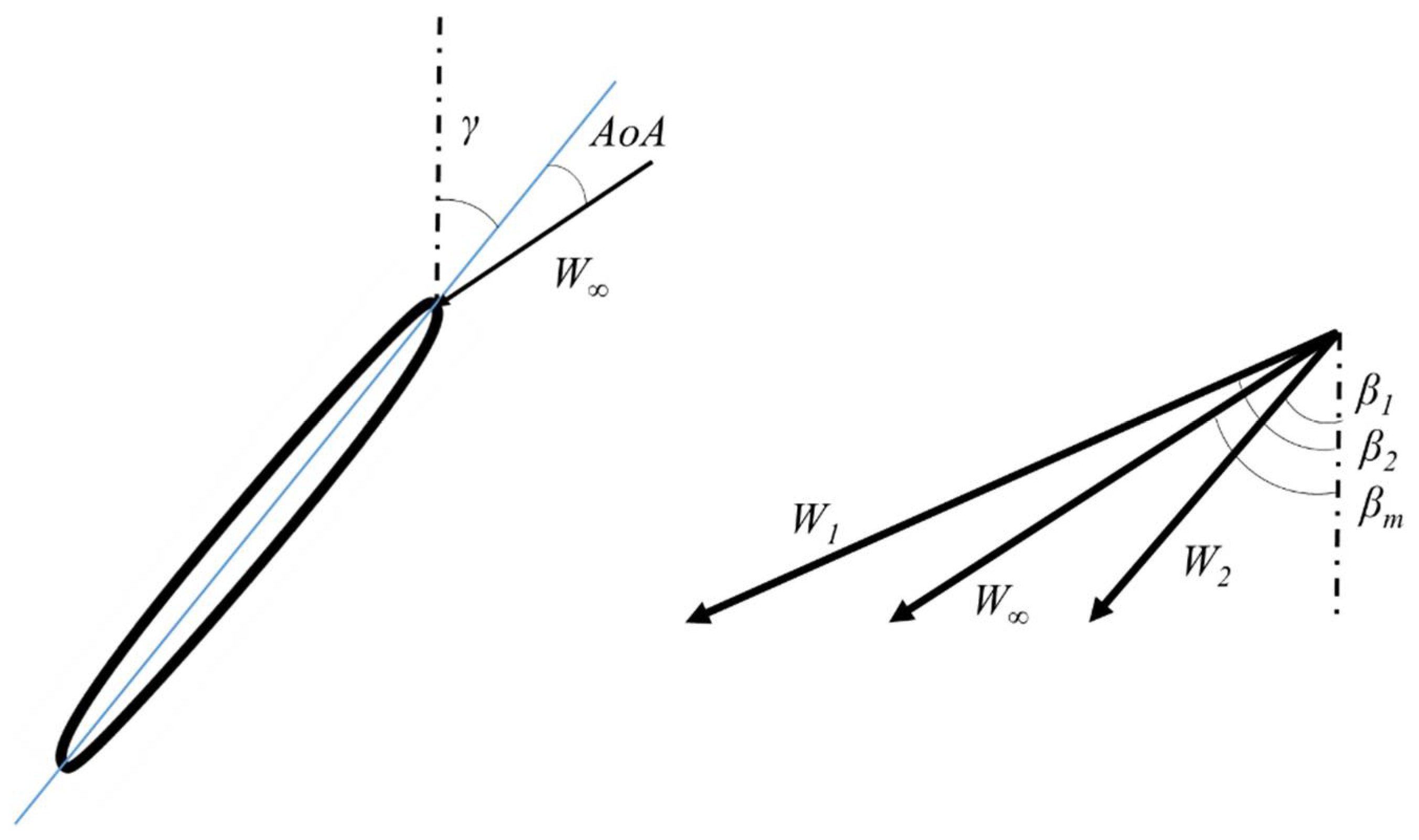
Such aerofoil collection can be used to re-stagger an existing fan blade to obtain better fan efficiency or more stable working conditions at a given design point. In fact, when velocity diagrams, aerodynamic loading (CL,i), Reynolds number (Rei), and blade solidity (σi) are prescribed at each blade radius, it is possible to determine the aerofoil stagger (γi) (Figure 2) that results in the blade working at optimized conditions ε′ and α′.
where “i” identifies the generic blade section along the span. The restaggered blade with optimized aerofoils will result in a deflection (θ = β/1 − β/1) close to the design deflection.
2.2. Aerofoil Parameterization
As the present study concerns truly reversible aerofoils, the parameterization of only one surface of the profile univocally defines the aerofoil geometry. Selection of the parameterization scheme among all available methods represents a crucial point, because it strongly influences the whole optimization process, as described by Wu [26], Kulfan [27], and Samareh [28]. For optimization purposes, the most important features of a parameterization scheme are the following: (i) to provide consistent geometry changes, and (ii) to produce an effective and compact set of design variables [28]. These two features are in fact fundamental during the optimization loop, because they simplify the generation and simulation of geometries, and avoid data overfitting in the meta-model. Two parameterization schemes were tested, Sobieczky [29] and the B-Splines parameterization [28]. These schemes were chosen for their simplicity and the reduced amount of design variables required to reproduce a set of given aerofoil geometries. B-Splines parameterization was selected according to its capability to reproduce the suction side of a set of 40 reversible aerofoils selected between the most commonly used in ventilation industry, or generated by a simple rearrangement of the suction side of several generic non-cambered aerofoils. A curve fitting algorithm, developed by Schneider [30], finds values of the parameterization coefficients for the given profiles to obtain the minimum deviation between a selected reversible aerofoil and the resulting parameterization.
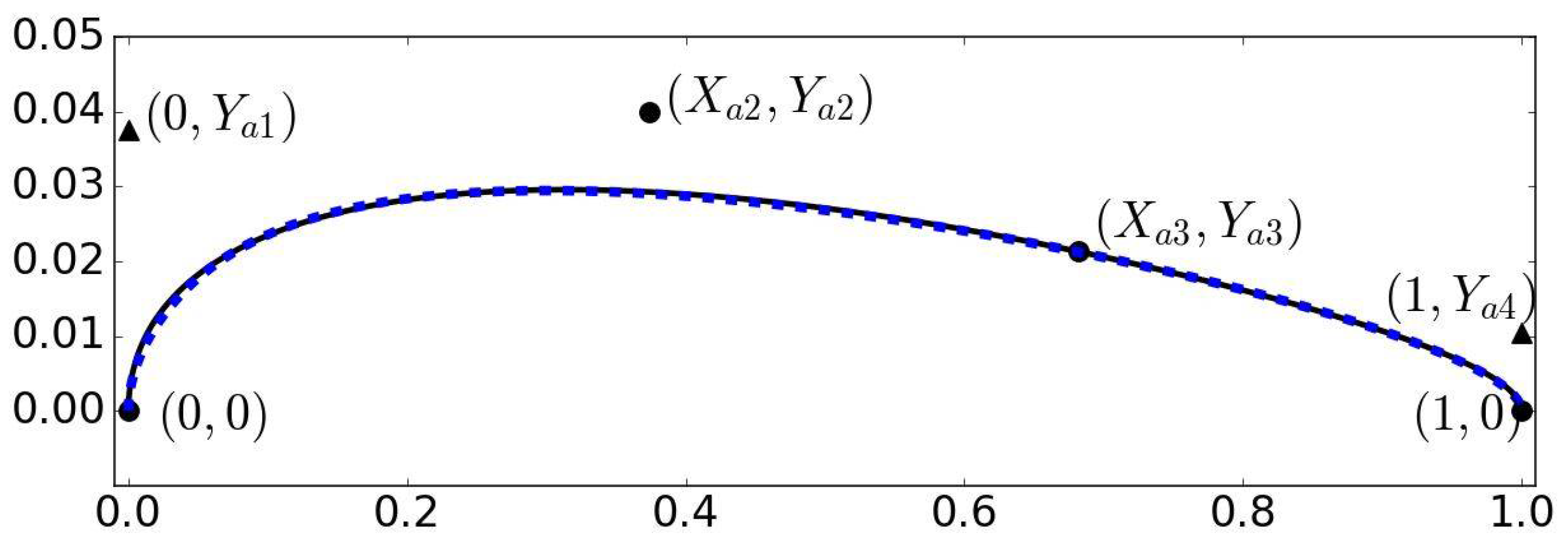
According to the Nelder–Mead search algorithm [31], the sixth degree B-Spline parameterization guarantees a good balance among aerofoil geometrical features and the number of design parameters. B-Spline parameterization uses the coordinates of six points. Two points define the beginning and the end of the aerofoil suction side and are forced to have coordinates (0, 0) and (1, 0). A second set of points indicates the direction of the surface at the leading edge and at the trailing edge. For those points, x was again forced to 0 and 1, respectively, while y coordinates are the first two degrees of freedom (Ya/1 and Ya/1). The third couple of points are used to control the suction surface between the leading and trailing edge, adding other four degrees of freedom (Xa2, Ya/1 and Xa/1, Ya/1). Figure 3 shows the set of control points and relative parameterization (dashed line) after the curve fit to reproduce the given geometry (solid line).
2.3. Optimization Algorithm
The MOOP has been solved using the non-dominated sorting genetic algorithm (NSGA-II) proposed by Deb [15]. NSGA-II is a non-dominated sorting-based multi-objective evolutionary algorithm (MOEA), combining the concept of non-dominated sorting together with an explicit diversity-preserving mechanism, based on crowding distance. Starting from the parent population Pt, taken as an initial set of N = 40 individuals (geometries), the algorithm generates an offspring population Qt of the same size N. Then, the two populations are combined to form an Rt population of size 2N. The offspring Qt is generated using the following criterion: four elements are generated using crossover, mutation, and breed interpolation from the first two most promising elements in Pt. Among them, the first two are random mutations, a third element is generated by scattered crossover, and the genes of the last element are averaged between the parents’ genes. The remaining 36 elements of Qt population are obtained by scattered crossover or mutation of random selected elements in Pt. A non-dominated sorting approach, as suggested by Deb [15], is used to pick individuals from the last non-dominated front. An advantage of this approach is that solutions compete with each other also in terms of how dense they are in the fitness space. Thus, diversity is explicitly considered when forming the offspring population. Furthermore, elitism is ensured by non-dominated sorting of both parents and offspring and inclusion of non-dominated fronts in the new set of elements. NSGA-II has demonstrated its ability to find a much better spread of solutions and better convergence near the true Pareto-optimal front when compared with the Pareto achieved with different evolutionary algorithms [24].
2.4. Test Matrix
We decided to select a series of operating conditions on the envelope of reversible fans for tunnel and metro applications [22]. A matrix of 25 optimization cases was defined by means of the selection of five values of Re, and five values of CLS, reported in Table 2. Each optimization starts from the same initial population (Pt) of N = 40 reversible aerofoils described above.
3. Surrogate Model-Based Optimizations
If the final objective is to compute a stable solution for the MOOP, more accurate and computationally expensive fitness estimators need to be deployed into the MOEA framework, increasing the time to solution. As a compromise, the established framework to address such challenging optimization problems is the use of surrogate-based optimization, in which a meta-model approximates the fitness function and leads the optimizer with local or global extrema values at a much lower computational cost [8,9]. In this work, the least square method (LSM) and artificial neural networks (ANNs) were used as surrogate models (SM) of the original BEM solution (i.e., the XFoil-based fitness function) in the MOOP.
Two meta-model optimization approaches were considered. Namely, the simple-level approach, in which the optimization is entirely driven by the SMs, and the bi-level approach, in which the reference solution (original fitness function) is used to evaluate the surrogate optimum designs.
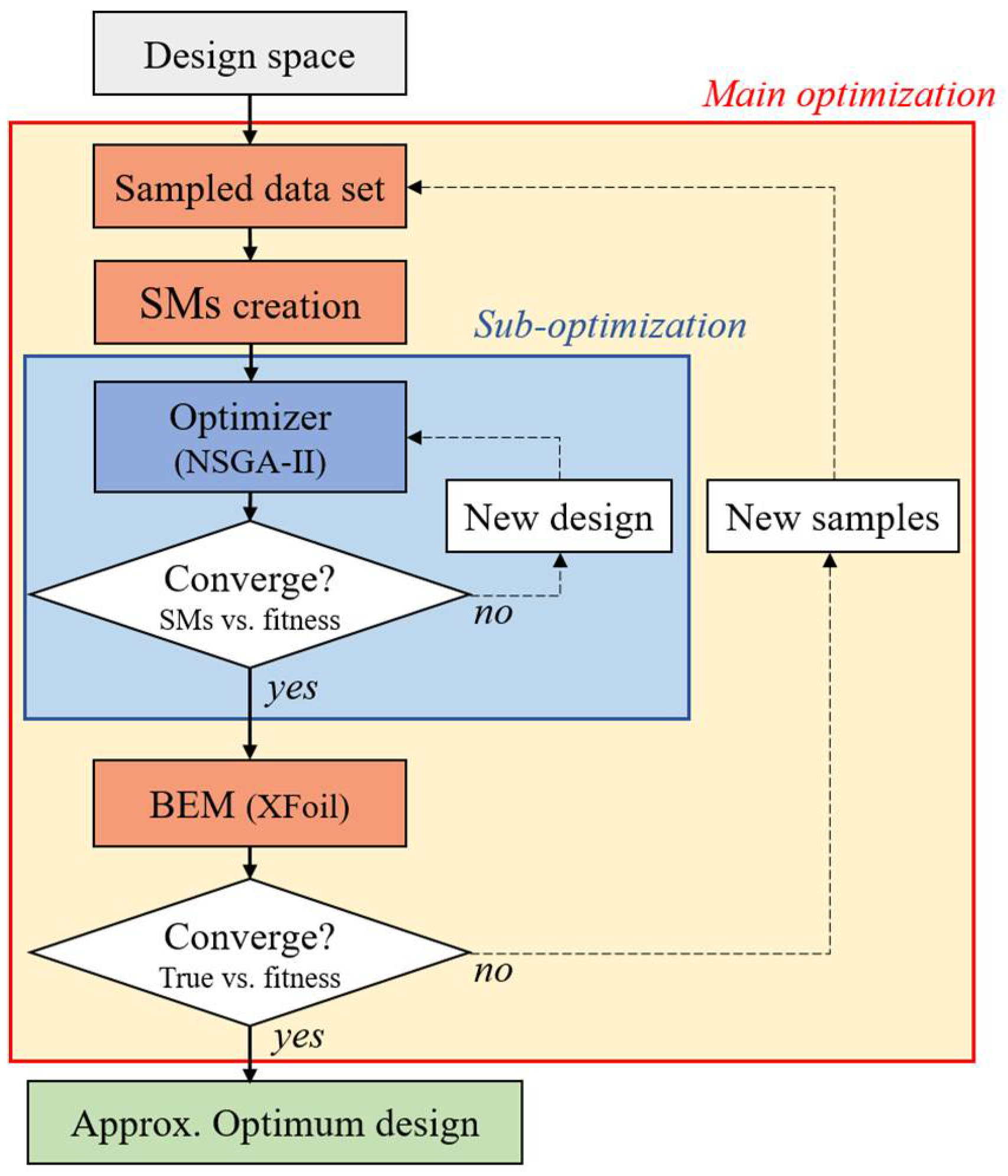
Following the classification proposed by Jin [32] and Manríquez [20], the simple-level is also called the direct fitness replacement (DFR) method or no evolution control (NEC), and it is considered the most straightforward SM approach. The simple-level framework is illustrated in Figure 4, where MOEAs calculate the solutions using the SMs without any assessment against the original fitness function. NEC has proven to be adequate in problems with low dimensionality in both decision and objective space, and is established in turbomachinery applications [11,12,13,14]. However, in more challenging problems [12,20], this approach can converge to false or sub-optima, which in a MOOP, is a Pareto front not corresponding to the Pareto front estimated by the original function.
The bi-level framework (or in-fill criterion), also known as the indirect fitness replacement (IFR) method [24,33], advocates the use of the fitness function during the EA process, adding new sample points to the current data set, while one or more components of the MOEA (typically the variation operators) are assessed in the SM. The IFR method is clearly a two-stage approach, as illustrated in Figure 5. A number of solutions are produced, evaluated, and compared using the SM. Among them, n best solutions are then delivered to the parent approach and evaluated against the original fitness function to enrich, iteration by iteration, the sampling data set from which meta-models are derived. Therefore, it is expected to keep the optimization towards the true Pareto front, and at the same time reduce the risk of convergence to false optima [16,34]. Most of the existing works in this category use the MOEA in a direct coarse grain search, while the SM intervenes in a local search, providing candidate solutions, which are then assessed in the real function. Therefore, the IFR approach uses the SM for exploitation purposes, while the MOEA is employed for design space exploration.
3.1. Data Sampling
In both of the optimization frameworks, the initial meta-models were trained by means of selected samples inside the design space. In this work, the design space includes s = 8 parameters (i.e., 6 airfoil geometry parameters, Re and CLS), and the vector of independent variables reads as follows:
Usually, a full factorial design of experiment is used to test all possible combinations of variables (factors). Such an approach would require a large number of experimental trials, specifically 38 = 6561. To reduce the number of trials, we use a central composite design, and in particular the rotatable central composite inscribed (CCI). CCI is full factorial, to which 2s axial trials and center point trials are added [35,36]. Axial points are located at factors levels −1 and 1, while factorial points are brought into the interior of the design space and located at distance 1/ν from the center point. Here, ν is the distance from the center of the design space to a star point. To ensure the rotatability of the design [37], ν was set to the following:
where s is the number of factors. As a consequence, the number of factorial runs is 28 = 256, with ν set to 4 to keep rotatability. The operating ranges for all the factors and the levels at which they were tested are shown in Table 3.
The total number of experimental trials was equal to N = 2s + 2s + 1 = 273. All 273 examples were tested by means of XFoil to calculate the vector of design objectives that reads as follows:
Notably, the entire sampling task required approximately 1.5 h on a 4 cores i7 laptop.
3.2. Least Square Method (LSM)
The model fitness function was approximated using a second-order polynomial response surface, which reads as follows:
A least square method fit approach enables the estimation of the polynomial coefficients, or regressors, so that it best fits the CCI data set. The polynomials (8) quantify the relationship between the vector O of the objective functions, ε and α, respectively, and the factors. ζι are the regressors and q is an error associated with the model. This first surrogate model is suitable for optimization processes and can handle noisy optimization landscapes, as reported in the works of [33,38].
3.3. Artificial Neural Network (ANN)
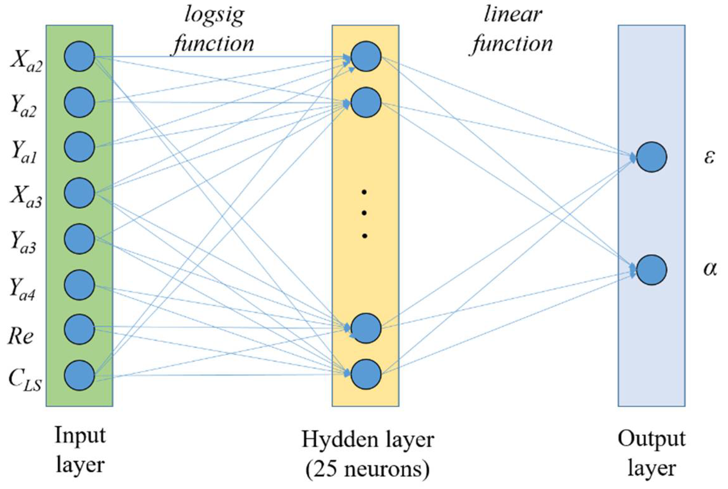
The neural network developed was a multilayer perceptron (MLP), commonly used in regression problems [39]. A series of tests on the architecture of the MLP was carried out to identify the best tradeoff architecture to ensure accuracy and limit the computational costs. Following these tests, the selected configuration MLP included one hidden layer, 25 neurons, a logsig activation function on the hidden layer, and a linear function on the output layer. Tests were done using 10 to 60 neurons, and 1 and 2 hidden layer(s), for a total of 6 tests on a single layer network and 36 tests on a double layer network. The architecture with one hidden layer and 25 neurons had the best surrogate model coefficient of determination. The MLP is illustrated in Figure 6.
The neural network was trained using a Bayesian optimization algorithm, randomly initializing weights and biases between 1 and −1. To avoid convergence into a local minimum and detect overfitting, the sampling dataset was re-organized into five different datasets; each was then split into a “training dataset” containing 80% of the total samples, and a “test dataset” with the remaining samples. The ANN was then trained on each dataset and the accuracy was evaluated by means of the coefficient of determination R/1, calculated above the entire normalized prevision set; ε and α.
3.4. Pareto Front Properties
To further analyze the SM-assisted multi-objective optimization performance, the quality of results was assessed using the following Pareto front properties: (i) the number of Pareto optimal solutions in the set; (ii) the accuracy of the solution in the set (i.e., measured by closeness to the theoretical Pareto-front solution); and (iii) the distribution and (iv) spread of the solutions [40]. To quantify these properties, we computed a set of performance indices. Specifically; (i) Overall Non-dominated Vector Generation Ratio (ONVGR); (ii) Hyperarea (H); and (iii) Spacing (Sp) and Overall Pareto Spread (OS).
ONVGR is a cardinality-based index derived from the one defined in Okabe et al. [40], and it is linked to the number of non-dominated solutions in the Pareto front. To compute this index, all the elements that populate the optimized solution sets (from all optimization framework; MOEA and SMs assisted optimizations) were combined in a unique Pareto front for each test case, according to the non-dominated sorting algorithm of NSGA-II. ONVGR defines the percentage of unique Pareto front elements that are generated from metamodel-assisted optimization, or using XFoil as fitness function. H identifies the area of objective space subtended by the Pareto solution set. Sp identifies the distance between the elements that populate the solution set. OS quantifies how widely the optimized solution set spreads over the objective space. In a two objectives optimization, it is computed as the ratio of the rectangle that is defined selecting the good and bad points (according to each objective functions), and the rectangle that has two vertices on the Pareto front extreme points. A solution set presenting higher OS value is characterized by wider spread.
4. Results
Standard MOEA results are first illustrated. The results from the developed SMs are then presented and compared against MOEA.
4.1. MOEA
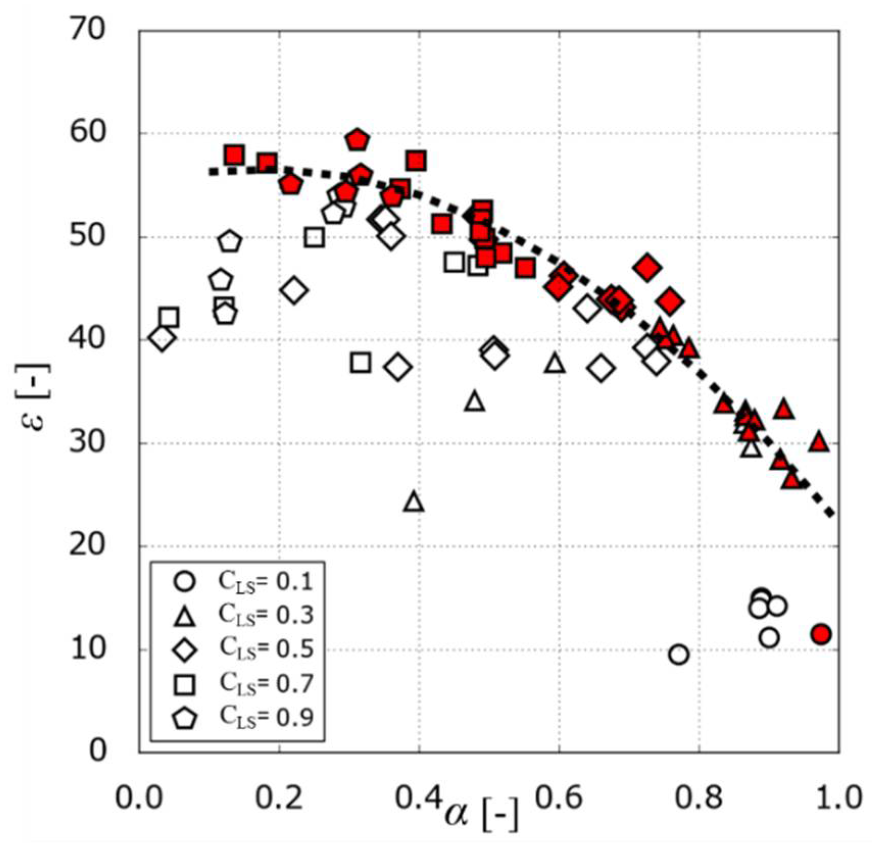
The fitness function selected to compute the objective functions ε and α during NSGA-II algorithm was based on BEM modelling of the airfoil (i.e. XFoil). This model was selected as it is customary in the prediction of aerofoil lift and drag polars [41,42]. Moreover, RANS-based numerical models were found to be affected by noise as a consequence of turbulence modelling discontinuous variations in calculating objective functions and discretization, as indicated by Giunta et al. [43] and Madsen et al. [44,45]. Figure 7 shows the objective function values of the initial given population Pt for Re = 1.05 × 10⁶ and CLS ranging between 0.1 and 0.9.
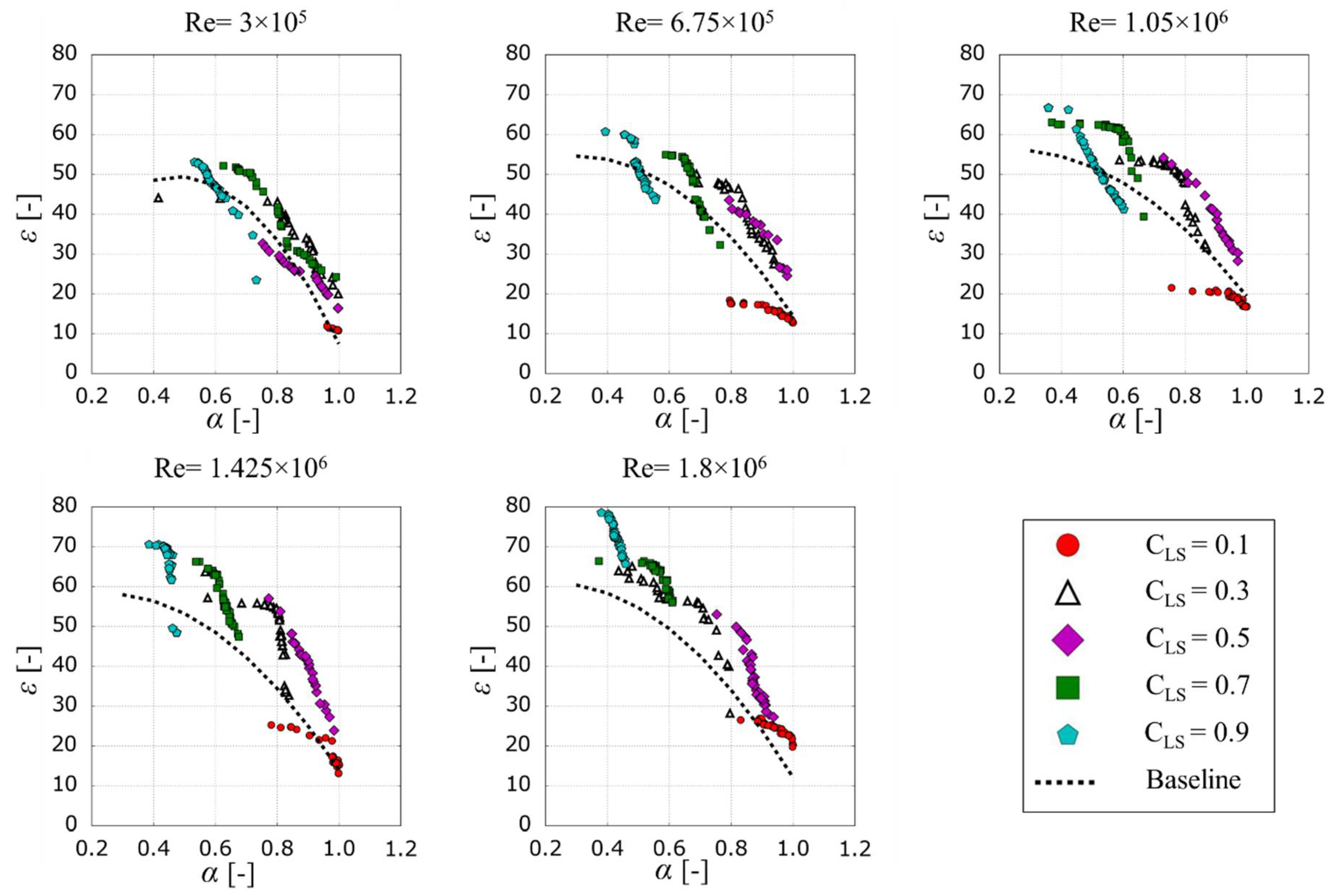
We analysed the initial population using XFoil with the aim to find an initial frontier. We sorted the tested individuals according to fast non-dominated sorting algorithm, suggested by Deb [15], obtaining the front depicted by filled symbols. Any optimization technique should move this imaginary frontier (dotted line) towards higher efficiencies and stall margins. Figure 8 shows the results for all Re and CLS combinations of the MOEA test matrix after 20 generations.
Each graph illustrates the initial frontier (dotted line) and the final frontier obtained by a selection of elements on the Pareto fronts. Irrespective of the configuration, the frontier shifts as a result of a major improvement in efficiency, lowering the stall margin.
4.2. No Evolution Control (NEC) or Single-Level Approach
MOOP was solved using NSGA-II algorithm assisted by developed meta-models. SMs’ accuracy in terms of coefficient of determination R/1 for the least square method and artificial neural networks is reported in Table 4.
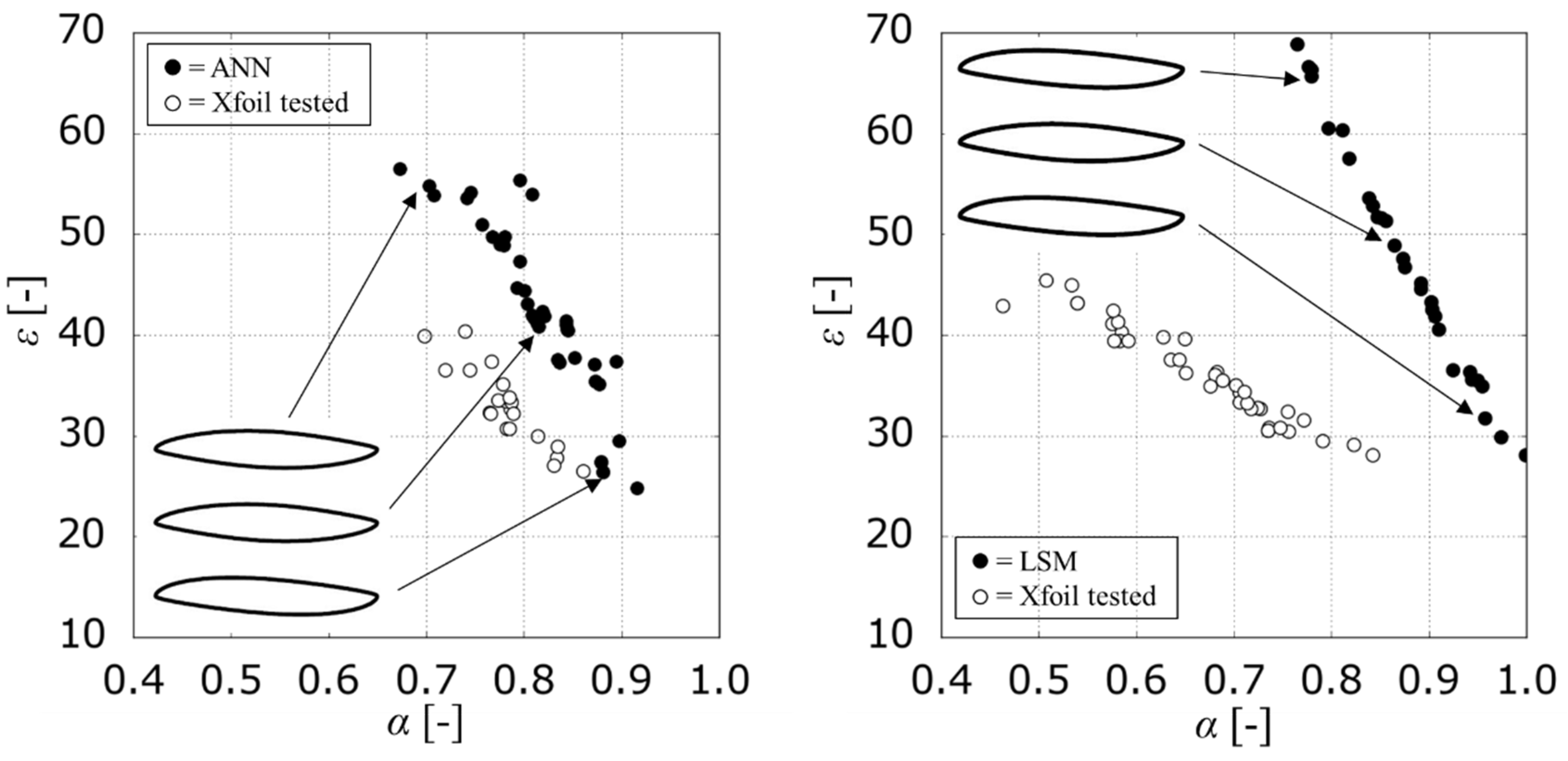
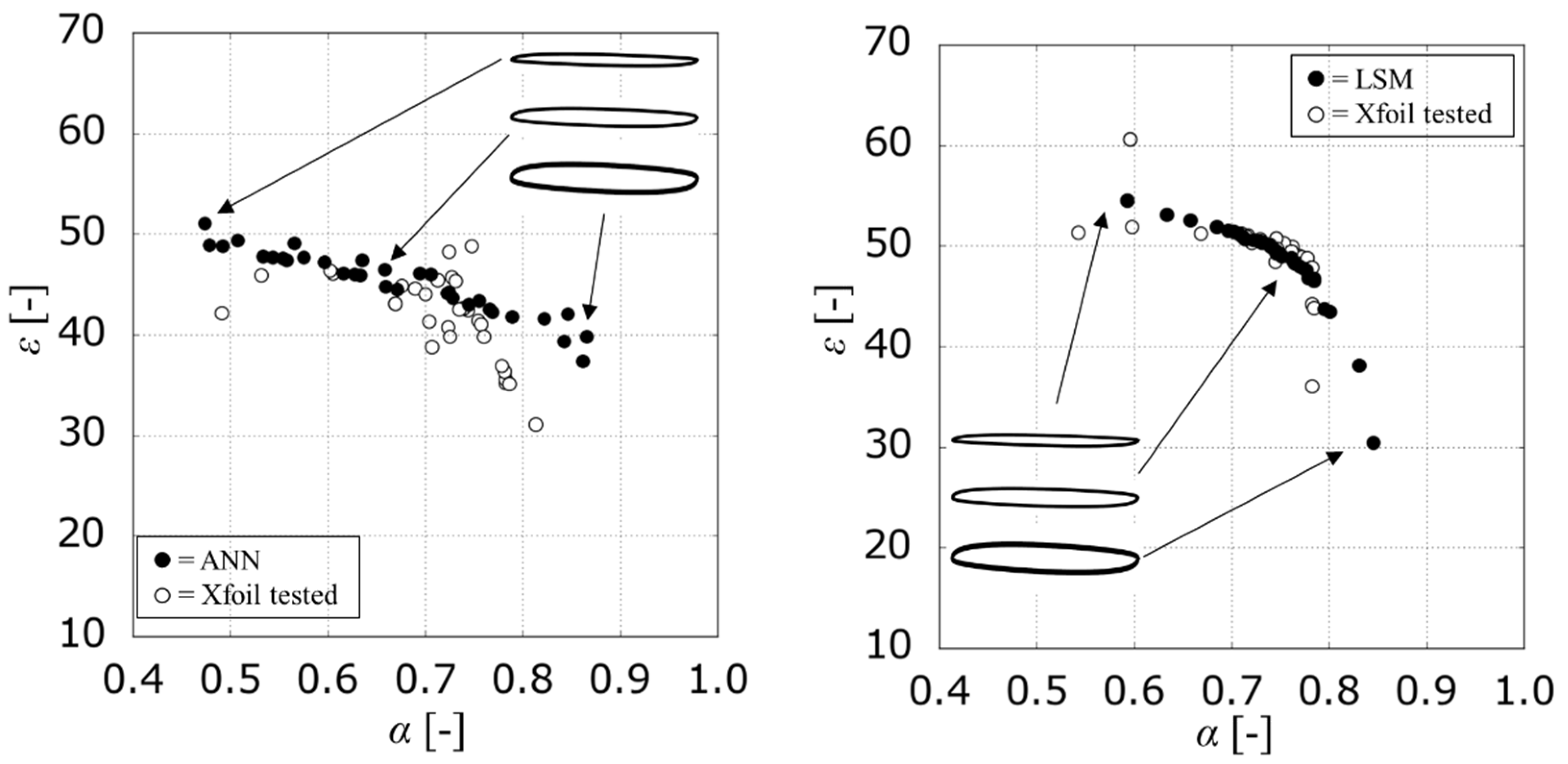
In this method, there is no call to the original fitness function-based BEM, and the optimization was stopped after 20 generations. To assess the results of the SM-assisted optimization, solutions on the Pareto fronts were retested with XFoil. Figure 9 shows the results of such an assessment for Re = 1.05 × 10⁶ and CLS = 0.5. Irrespective of the value of Reynolds number and CLS, the use of SMs to drive the optimization result was inadequate with the NEC approach. In fact, a consistent discrepancy was observed between the meta-model predicted aerodynamic performance (black dots) and the performance obtained testing the same individuals with the BEM function (white dots).
A geometrical analysis made on a few geometries of the SMs’ Pareto fronts confirms that the geometrical trends, previously found with MOEA, are not reproduced. In addition, as described in Figure 9, each Pareto front given by SMs provides similar aerofoil shape, in contrast to the flow physics, which suggest the finding of thinner aerofoils in zones with high efficiency and low stall margin, and conversely an increased thickness in the zone with low efficiency and high stall margin.
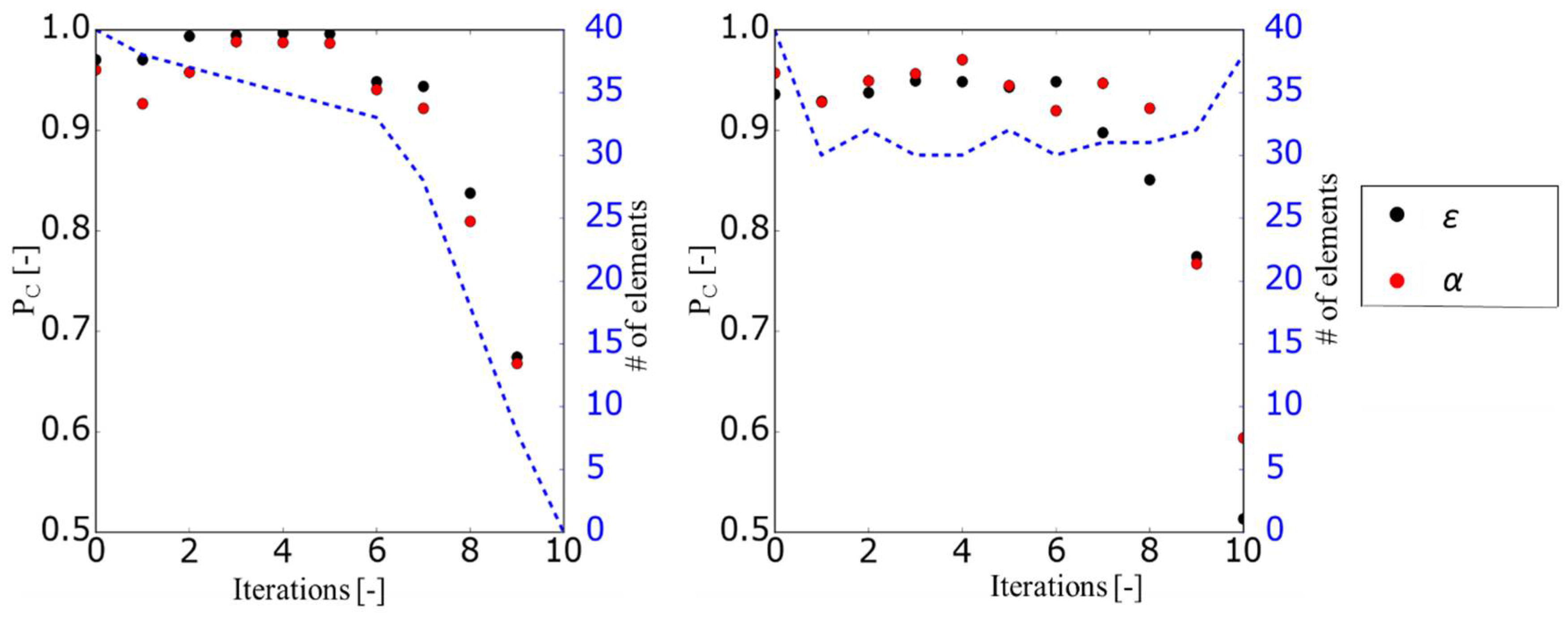
To quantify the underlined departure of SMs’ optimization, the prediction capability (Pc) was plotted against the number of iterations in Figure 10 (i.e., Re = 1.05 × 10⁶, CLS = 0.5). Notably, the prediction capability Pc is an index similar to the coefficient of determination R/1, computed as follows:
where εBEM,i is the aerodynamic efficiency (objective function) of the ith individual of Pareto front tested with the BEM function, and ε,i is the efficiency predicted by the surrogate model. Using the same criteria, we have computed Pc,α.
Irrespective of the SMs, after an initial phase of five or six iterations, in which the meta-model prediction is above 90%, Pc quickly drops for both objectives ε and α. Despite that Pc trends in ANN and LSM are similar, the optimization behaviors are totally different. In the test matrix, ANN tends to empathize a geometrical feature that generates distorted or unrealistic geometries that are hard or impossible to simulate by means of XFoil, while this trend was seldom recorded for LSM.
The inability of meta-model based optimized geometry to replicate the behaviour of aerofoils is strongly connected to the incorrect prediction of elements in the intermediate regions of the sampled design space for SMs’ instruction. This circumstance was already documented in highly dimensional problems (as in the present case owing to the selected aerofoil parameterization) when using the single-level NEC approach [12,46].
4.3. Indirect Fitness Replacement (IFR) or Bi-Level Approach
In view of the poor performance of the NEC approach, the IFR framework was implemented for the solution of the MOOP. In this case, the initial sampling was used to train the first iteration of both meta-models. Then, meta-model assisted NSGA-II was invoked for five generations. The genetic algorithm was kept identical to the original formulation used in the reference MOEA optimization. After the NSAG-II completion, the 40 best new members are evaluated using the original fitness objective function, and then stored to enrich the SMs training pool. To this end, a limit of 10 calls to the objective function was set, in order to control the computational cost of the optimization process.
Figure 11 illustrates the results of the final iteration loop again for the combination Re = 1.05 × 10⁶, CLS = 0.5, already used in the NEC exploration. In the IFR approach, aerodynamic performance predictions are in good agreement with XFoil predictions, with a significant gap reduction between Pareto fronts estimated by the meta-models and by the original fitness function. In addition, it is possible to infer that the aerofoil flow physics is well represented in both SM-based optimizations, by the change in the aerofoils geometry. Thinner aerofoils populate the upper left region of Pareto front, where the efficiency increases to the detriment of stall margin, as expected and confirmed by MOEA analysis.
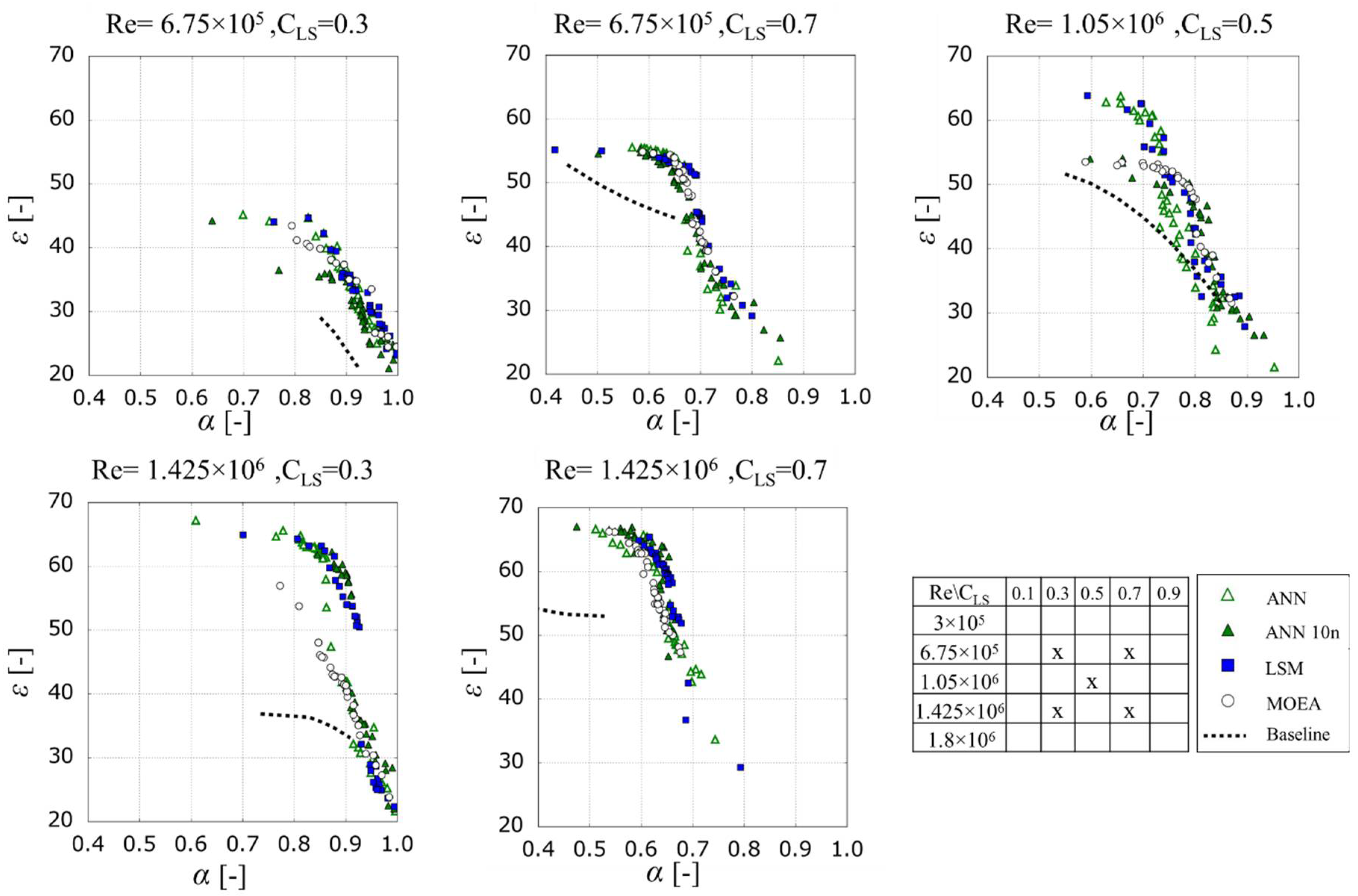
Figure 12 shows the overall comparison of SM-assisted optimizations against the standard MOEA for five different configurations of the test matrix. Notably, in Figure 12, the dotted lines indicate the base-line aerofoil performance for the specified Re and CLS values. To give additional hints about the ANN-based surrogate, Figure 12 also shows the results of a reduced complexity level artificial neural network with only 10 neurons per hidden layer. Because the results obtained with the IFR approach demonstrates that the complexity of SMs had low impact on the quality of the obtained Pareto fronts, we performed the optimization with a simplified version of the ANN to reduce the computational effort required. At a glance, these results give the indication of the quality of SM-assisted optimizations implemented in a IFR test-bed, using half of the computational effort required by the MOEA. It is also worth noting that, when comparing the two meta-models, the quality of the Pareto front solutions is close, indicating a reduced influence of the optimization process to the specific meta-modelling algebra.
Table 5 reports the values of the indexes described in Section 3.4. In each column, the best case is in bold, and the worst case is in italic.
According to the values of ONVGR listed in Table 5, the SM-assisted optimizations resulted in a larger number of non-dominated elements in the set when compared with MOEA. The only exception concerns the central test case in the matrix (Re = 105000, CLS = 0.5), where MOEA optimization reaches 33.3% of non-dominated elements. However, we can obtain the same result using LSM as the fitness function.
As per H, the use of ANN determines a wider dominated area in the objective space, although LSM has very close values for the same test cases. As observed above, also in this case, worse results have been obtained using the MOEA approach. Concerning SP values, the analysis shows that ANN, even with 10 neurons, in general have Pareto fronts characterized by the minimum distance between the elements that populate the solution. The values of OS tend to confirm that ANN Pareto sets present a wider spread over the objective space, in line with the H quality.
As a final comment, it is impossible to say that the overall quality of solution sets for MOOP cannot be accounted for by means of a single performance index, especially if the shape of Pareto front is extremely different. In the end, because in this study the declared final objective was to move as much as possible the technological frontier on the α–ε chart, the effectiveness was assessed by means of ONGVR index, concluding that SMs-assisted optimization can be equivalent, or even better in this case, with respect to that based on XFoil and surrogate models.
5. Conclusions
This paper presents an investigation of surrogate-based optimization of truly reversible profile family for axial fans. The multi-objective optimization problem (MOOP) is based on the NSGA-II, an evolutionary algorithm able to find multiple Pareto-optimal solutions in one simulation run. The MOOP has been firstly solved using the XFoil software, avoiding the modelling and use of any SMs. These results have been compared with those obtained by implementing different SMs in the MOOP, considering two different optimization frameworks, namely NEC and IFR.
The use of SMs to assist MOEAs is a complex matter that requires an exhaustive analysis of the entire optimization framework and how the SMs are embedded in the considered optimization algorithm.
This work has shown that, for this problem, an IFR approach has to be preferred to an NEC approach. In fact, an NEC approach has produced false Pareto-fronts in all of the tested configurations. In particular, the NEC optimization has been not able to explore the entire design space in between the sampling points. The genetic algorithm led the optimizer to candidate solutions that were, during every iteration, more and more distant from the corresponding true value. This interpretation was suggested by the decreasing value of prediction capability associated with the increase of unrealistic geometries and thick profile.
An IFR approach has produced more reliable results, providing a good prediction capability during the iterations, and hence reducing the distance between estimated and true Pareto fronts. The optimization was able to cover the entire design space, providing a geometry along the Pareto fronts similar to those experienced by the MOEA optimization. The IFR method required a more complex and computationally expensive optimization framework based on a bi-level approach, with the infill criterion based on the results of the GA.
An analysis of the ONVGR index has shown that, in most cases, the IFR optimization was able to produce better results (individuals) than the XFoil-based optimization.
Regarding the SMs used in this work (an LSM and ANN with different number of neurons), the IFR results show the independence of the MOEA to the SM considered. This is considered an important outcome; LSM being an easier and faster to model when compared with an ANN. On the other side, the NEC approach results do not present any relevant differences between the two SMs, even though different prediction accuracies were reached.
The different reliability of the results obtained by adopting a NEC and IFR approach scales down the role and importance of the initial sampling in SMs-based optimization. In fact, it is evident that an NEC approach is totally favourable to exploitation, on the contrary, not being able to correctly explore the design space. An IFR approach, which involves an infill criterion, overcomes the difficulties and limitations related to the correct initial sampling creation, by iteratively adding optimized solutions evaluated with XFoil to the initial sampling. This approach ensures a better balance between exploration and exploitation of the design space.
The results shown for the IFR approach demonstrated that, in the selected cases, a consistent reduction of MOOP computational cost is possible. In the specific case, according to the metric selected to judge the Pareto frontiers, the calls to the expensive objective function were reduced by 50%, in all cases producing a reliable set of better solutions in comparison with the standard MOEA approach.
In conclusion, this study clarified the strong impact of the optimization framework on the reliability of the obtained Pareto fronts in a SM-based design optimization for an industrial fan benchmark problem. With an IFR approach, the use of the considered SMs can significantly reduce the computational time needed to solve the MOOP by reducing the call of the fitness function, while ensuring the creation of the same, or even better, Pareto fronts when compared with those obtained using only XFoil. The solutions obtained by the IFR method present higher values of Pareto quality indexes when compared with MOEA (see Table 5). The major improvement is associated with the ONVGR index, which assesses that the elements populating the Pareto front obtained with the SMs-assisted optimization dominate the solution obtained with the MOEA.
Nomenclature
| Acronyms | ||
| ANN | Artificial Neural Network | |
| CCD | Central Composite Design | |
| CCI | Central Composite Inscribed | |
| CFD | Computational Fluid Dynamic | |
| DFR | Direct Fitness Replacement | |
| EAs | Evolutionary Algorithms | |
| FNDS | Fast non dominated sorting algorithm | |
| GAs | Genetic Algorithms | |
| H | Dominated Space or Hyperarea | |
| IFR | Indirect Fitness Replacement | |
| LSM | Least Square Method | |
| MOEA | Multi-Objectives Evolutionary Algorithms | |
| MOOPs | Multi-Objectives Optimization Problems | |
| MS | Max Sum | |
| NSGA-II | Non-dominated sorting genetic algorithm | |
| NEC | No Evolution Control | |
| ONVGR | Overall Non-dominated Vector Generation Ratio | |
| Qt | Offspring population | |
| OS | Overall Pareto Spread | |
| PC | Prediction capability | |
| Pt | Initial population | |
| Rt | Global population | |
| SMs | Surrogate Models | |
| SP | Spacing | |
| Latin | ||
| a, z | Synapse activity | [-] |
| AoA | Angle of attack | [deg] |
| CD | Drag coefficient | [-] |
| CL | Lift coefficient | [-] |
| CLS | Specified lift coefficient | [-] |
| g | Array containing aerofoil geometry | [-] |
| k | Neuron number | [-] |
| m | ANN number of predicted dependent variables | [-] |
| q | LSM associated error | [-] |
| Re | Reynolds number | [-] |
| s | LSM number of factors | [-] |
| W | Relative velocity | [m/s] |
| F | factors | [-] |
| Xai | x-coordinates of B-Spline parameterization | [-] |
| O | objectives | [-] |
| Yai | y-coordinates of B-Spline parameterization | [-] |
| Symbols | ||
| α | Stall margin | [-] |
| β | Flow angle | [deg] |
| γ | Aerofoil stagger | [deg] |
| ε | Aerodynamic efficiency | [-] |
| ζi | LSM regressors | [-] |
| θ | Deflection | [deg] |
| λ | Linear activation function | [-] |
| ν | Star point distance | [-] |
| σ | Sigmoid activation function | [-] |
| Superscripts | ||
| ‘ | Selected solution | |
| 1,2 | Inlet and Outlet fan sections |
References
- Sheard, G.; Daneshkhah, K. The Conceptual Design of High Pressure Reversible Axial Tunnel Ventilation Fans. Adv. Acoust. Vib. 2012, 2012. [Google Scholar] [CrossRef]
- Bolton, A.N. Installation effects in fan systems. Proc. Inst. Mech. Eng. Part A J. Power Energy 1990, 204, 201–215. [Google Scholar] [CrossRef]
- Cardillo, L.; Corsini, A.; Delibra, G. A numerical investigation into the aerodynamic effect of pressure pulses on a tunnel ventilation fan. Proc. Inst. Mech. Eng. Part A J. Power Energy 2014, 228, 285–299. [Google Scholar] [CrossRef]
- William, C. Fans and Ventilation: A Practical Guide; Elsevier: New York, NY, USA, 2010. [Google Scholar]
- Herrig, L.J.; Emery, J.C.; Erwin, J.R. Systematic Two-Dimensional Cascade Tests of Naca 65-Series Compressor Blades At Low Speeds; National Advisory Committee for Aeronautics: Washington, DC, USA, 1957. [Google Scholar]
- Lieblein, S.; Ackley, R.H. Secondary Flows in Annular Cascades and Effects on Flow in Inlet Guide Vanes; National Advisory Committee for Aeronautics: Washington, DC, USA, 1951. [Google Scholar]
- Marler, R.T.; Arora, J.S. Survey of multi-objective optimization methods for engineering. Struct. Multidiscip. Optim. 2004, 26, 369–395. [Google Scholar] [CrossRef]
- Forrester, A.I.J.; Keane, A.J. Recent advances in surrogate-based optimization. Prog. Aerosp. Sci. 2009, 45, 50–79. [Google Scholar] [CrossRef] [Green Version]
- Queipo, N.V.; Haftka, R.T.; Shyy, W.; Goel, T. Surrogate-based analysis and optimization. Prog. Aerosp. Sci. 2005, 41, 1–28. [Google Scholar] [CrossRef] [Green Version]
- Jang, C.M.; Kim, K.Y. Optimization of a stator blade using response surface method in a single-stage transonic axial compressor. Proc. Inst. Mech. Eng. Part A J. Power Energy 2005, 219, 595–603. [Google Scholar] [CrossRef]
- Bamberger, K.; Carolus, T. Performance Prediction of Axial Fans by CFD-Trained Meta-Models. In Proceedings of the ASME Turbo Expo 2014: Turbine Technical Conference and Exposition, Düsseldorf, Germany, 16–20 June 2014. [Google Scholar]
- Gonzalez, L.; Periaux, J.; Srinivas, K.; Whitney, E. A generic framework for the design optimisation of multidisciplinary UAV intelligent systems using evolutionary computing. In Proceedings of the 44th AIAA Aerospace Sciences Meeting and Exhibit, Reno, Nevada, 9–12 January 2006; pp. 1–19. [Google Scholar]
- Kim, J.H.; Choi, J.H.; Husain, A. Multi-objective optimization of a centrifugal compressor impeller through evolutionary algorithms. Proc. Inst. Mech. Eng. Part A J. Power Energy 2010, 224, 711–721. [Google Scholar] [CrossRef]
- Deb, K.; Pratap, A.; Agarwal, S. Response surface approximation of Pareto optimal front in multi-objective optimization. Comput. Methods Appl. Mech. Eng. 2007, 196, 879–893. [Google Scholar]
- Deb, K.; Pratap, A.; Agarwal, S. A fast and elitist multiobjective genetic algorithm: NSGA-II. IEEE Trans. Evol. Comput. 2002, 6, 182–197. [Google Scholar] [CrossRef] [Green Version]
- Arias-Montano, A.; Coello, C.A.C.; Mezura-Montes, E. Multi-objective airfoil shape optimization using a multiple-surrogate approach. In Proceedings of the 2012 IEEE Congress on Evolutionary Computation (CEC), Brisbane, Australia, 10–15 June 2012; pp. 1–8. [Google Scholar]
- Samad, A.; Kim, K.Y. Shape optimization of an axial compressor blade by multi-objective genetic algorithm. Proc. Inst. Mech. Eng. Part A J. Power Energy 2008, 222, 599–611. [Google Scholar] [CrossRef]
- Tenne, Y. Initial sampling methods in metamodel-assisted optimization. Eng. Comput. 2015, 31, 661–680. [Google Scholar] [CrossRef]
- Jin, R.; Chen, W.; Sudjianto, A. An efficient algorithm for constructing optimal design of computer experiments. J. Stat. Plan. Inference 2005, 134, 268–287. [Google Scholar] [CrossRef]
- Toscano, T.G.; Barron-Zambrano, J.H.; Tello-Leal1, E. A review of surrogate assisted multiobjective evolutionary algorithms. Comput. Intell. Neurosci. 2016, 2016. [Google Scholar] [CrossRef]
- Drela, M.; Youngren, H. ‘X-Foil 6.96’ Software. Available online: web.mit.edu/drela/Public/web/xfoil (accessed on 30 November 2001).
- Daly, B.B. Woods Practical Guide to Fan Engineering; Woods of Colchester Limited: Colchester, UK, 1978. [Google Scholar]
- Oliphant, T. Python for Scientific Computing. Comput. Sci. Eng. 2007. [Google Scholar] [CrossRef]
- Angelini, G.; Bonanni, T.; Corsini, A.; Delibra, G.; Tieghi, L.; Volponi, D. A Meta-Model for Aerodynamic Properties of a Reversible Profile in Cascade with Variable Stagger and Solidity. In Proceedings of the 2018 ASME Turbo Expo, Oslo, Norway, 9–13 June 2018. [Google Scholar]
- Drela, M. An analysis and design system for low Reynolds number airfoil aerodynamics. In Proceedings of the Low Reynolds Number Airfoil Aerodynamics, Notre Dame, IN, USA, 5–7 June 1989. [Google Scholar]
- Wu, Y.H.; Yang, C.; Liu, F.; Tsai, M. Comparison of three geometric representations of airfoils for aerodynamic optimization, AIAA 2003-4095. In Proceedings of the 16th AIAA CFD Conference, Orlando, FL, USA, 23–26 June 2003. [Google Scholar]
- Kulfan, M.B.; Bussoletti, J.E. Fundamental parametric geometry representations for aircraft component shapes. In Proceedings of the 11th AIAA/Issmo Multidisciplinary Analysis and Optimization Conference, Portsmouth, Virginia, 6–8 September 2006. [Google Scholar]
- Samareh, J.A. Survey of shape parameterization techniques for high-fidelity multidisciplinary shape optimization. AIAA J. 2001, 39, 877–884. [Google Scholar] [CrossRef]
- Sobieczky, H. Parametric Airfoils and Wings, Notes on Numerical Fluid Mechanics; Vieweg Verlag: Wiesbaden, Germany, 1998; Volume 68, pp. 71–78. [Google Scholar]
- Schneider, P.J. An Algorithm for Automatically Fitting Digitized Curves. Graphics Gems; Academic Press Professional, Inc.: Cambridge, MA, USA, 1990. [Google Scholar]
- Inger, S.; Nelder, J. Nelder-mead algorithm. Scholarpedia 2009, 4, 2928. [Google Scholar] [CrossRef]
- Jin, Y. A comprehensive survey of fitness approximation in evolutionary computation. Soft Comput. A Fusion Found. Methodol. Appl. 2005, 9, 3–12. [Google Scholar] [CrossRef] [Green Version]
- Jin, R.; Chen, W.; Simpson, T.W. Comparative studies of metamodelling techniques under multiple modelling criteria. Struct. Multidiscip. Optim. 2001, 23, 1–13. [Google Scholar] [CrossRef]
- Adra, S.F.; Griffin, I.; Fleming, P.J. An informed convergence accelerator for evolutionary multiobjective optimiser. In Proceedings of the 9th Annual Conference on Genetic and Evolutionary Computation, London, UK, 7–11 July 2007; pp. 734–740. [Google Scholar]
- Montgomery, D.C. Design and Analysis of Experiments; John Wiley & Sons, Inc.: Hoboken, NJ, USA, 2001; p. 456. [Google Scholar]
- Wilkie, D. The design of experiments for engineering studies with particular reference to thermofluids. Proc. Inst. Mech. Eng. Part A J. Power Energy 1991, 205, 67–76. [Google Scholar] [CrossRef]
- Box, G.E.P.; Hunter, J.S.; Hunter, W.G. Statistics for Experimenters: Design, Innovation, and Discovery; Wiley-Interscience: Hoboken, NJ, USA, 2005; pp. 47, 455. [Google Scholar]
- Jin, R.; Du, X.; Chen, W. The use of metamodeling techniques for optimization under uncertainty. Struct. Multidiscip. Optim. 2003, 25, 99–116. [Google Scholar] [CrossRef] [Green Version]
- Hagan, M.T.; Demuth, H.B.; Beale, M.H. Neural Network Design; PWS Pub: Boston, MA, USA, 1996. [Google Scholar]
- Okabe, T.; Jin, Y.; Sendhoff, B. A critical survey of performance indices for multi-objective optimisation. In Proceedings of the 2003 Congress on Evolutionary Computation, Canberra, ACT, Australia, 8–12 December 2003; pp. 878–885. [Google Scholar]
- Cencelli, N.A. Aerodynamic Optimisation of a Small-Scale Wind Turbine Blade for Low Windspeed Conditions. Master’s Thesis, Stellenbosch University, Stellenbosch, South Africa, 2006. [Google Scholar]
- Van der Spuy, S.J.; von Backström, T.W. An evaluation of simplified cfd models applied to perimeter fans in air-cooled steam condensers. Proc. Inst. Mech. Eng. Part A J. Power Energy 2015, 229, 948–967. [Google Scholar] [CrossRef]
- Giunta, A. A Noisy aerodynamic response and smooth approximations in HSCT design. In Proceedings of the 5th Symposium on Multidisciplinary Analysis and Optimization, Panama City Beach, FL, USA, 1994; pp. 1117–1128. [Google Scholar]
- Madsen, J.I.; Shyy, W.; Haftka, R.T. Response surface techniques for diffuser shape optimization. AIAA J. 2000, 38, 1512–1518. [Google Scholar] [CrossRef]
- Li, J.Y.; Li, R.; Gao, Y.; Huang, J. Aerodynamic optimization of wind turbine airfoils using response surface techniques. Proc. Inst. Mech. Eng. Part A J. Power Energy 2010, 224, 827–838. [Google Scholar] [CrossRef]
- Choi, S.; Alonso, J.J.; Chung, H.S. Design of a low-boom supersonic business jet using evolutionary algorithms and an adaptive unstructured mesh method. AIAA Paper 2004, 1758, 2004. [Google Scholar]
Figure 1.
Reversible aerofoil generation.

Figure 2.
Definition of blade angle of attack (AoA), stagger angle (γ), and relative velocities.

Figure 3.
Control points used to reproduce the given geometry (solid line) with a sixth degree B-Spline parameterization (dashed line).
Figure 3.
Control points used to reproduce the given geometry (solid line) with a sixth degree B-Spline parameterization (dashed line).

Figure 4.
Direct fitness replacement (DFR) or simple-level optimization framework. SMs—surrogate models; NGSA—non-dominated sorting genetic algorithm.
Figure 4.
Direct fitness replacement (DFR) or simple-level optimization framework. SMs—surrogate models; NGSA—non-dominated sorting genetic algorithm.

Figure 5.
Indirect fitness replacement (IFR) or bi-level optimization framework. BEM—boundary element method.
Figure 5.
Indirect fitness replacement (IFR) or bi-level optimization framework. BEM—boundary element method.

Figure 6.
Neural network structure.

Figure 7.
Original fitness function objectives ε and α for Re 1.05 × 10⁶ and different values of CLS. Filled symbols are used to interpolate a technological frontier (dotted line) for the baseline aerofoil geometries.
Figure 7.
Original fitness function objectives ε and α for Re 1.05 × 10⁶ and different values of CLS. Filled symbols are used to interpolate a technological frontier (dotted line) for the baseline aerofoil geometries.

Figure 8.
Pareto fronts for Re from 3 × 10⁵ to 1.8 × 10⁶, and CLS from 0.1 to 0.9.

Figure 9.
Final iteration (in black dots) and its XFoil verification (white dots) for the NEC approach for artificial neural networks (left) and the least square method (right) for Re 1.05 × 10⁶ and CLS 0.5.
Figure 9.
Final iteration (in black dots) and its XFoil verification (white dots) for the NEC approach for artificial neural networks (left) and the least square method (right) for Re 1.05 × 10⁶ and CLS 0.5.

Figure 10.
Prediction capability progression and optimized elements generated during the first 10 generations for both objective functions for Re = 1.05 × 10⁶ and CLS =0.5. Left: ANN; Right: LSM.
Figure 10.
Prediction capability progression and optimized elements generated during the first 10 generations for both objective functions for Re = 1.05 × 10⁶ and CLS =0.5. Left: ANN; Right: LSM.

Figure 11.
Final iteration (in black dots) and its XFoil verification (white dots) for IFR approach for artificial neural networks (left) and the least square method (right) for Re = 1.05 × 10⁶ and CLS = 0.5.
Figure 11.
Final iteration (in black dots) and its XFoil verification (white dots) for IFR approach for artificial neural networks (left) and the least square method (right) for Re = 1.05 × 10⁶ and CLS = 0.5.

Figure 12.
Pareto fronts for five different test matrix configurations.


Table 1.
B-Spline parameterization error range.
| min error | 4.29 × 10⁻⁵ |
| max error | 7.26 × 10⁻⁴ |
| mean error | 2.91 × 10⁻⁴ |
Table 2.
Reynolds (Re) and specified value of lift coefficient (CLS) values used in the test matrix.
Table 2.
Reynolds (Re) and specified value of lift coefficient (CLS) values used in the test matrix.
| Re | 300,000 | 675,000 | 1,050,000 | 1,425,000 | 1,800,000 |
| CLS | 0.1 | 0.3 | 0.5 | 0.7 | 0.9 |
Table 3.
Tested levels of design variables.
| Variable | Coded Levels and Corresponding Absolute Levels | ||||
|---|---|---|---|---|---|
| −1 | −1/ν | 0 | 1/ν | 1 | |
| Xa/1 | 0.0140 | 0.0282 | 0.0330 | 0.0377 | 0.0519 |
| Ya/1 | 0.0217 | 0.0423 | 0.0491 | 0.0560 | 0.0765 |
| Ya/1 | 0.0126 | 0.0332 | 0.0401 | 0.0470 | 0.0676 |
| Xa/1 | 0.0049 | 0.0136 | 0.0164 | 0.0193 | 0.0280 |
| Ya/1 | 0.2761 | 0.3430 | 0.3653 | 0.3876 | 0.4545 |
| Ya/1 | 0.0265 | 0.0599 | 0.0710 | 0.0821 | 0.1155 |
| Re | 300,000 | 862,500 | 1,050,000 | 1,237,500 | 1,800,000 |
| CLS | 0.1 | 0.4 | 0.5 | 0.6 | 0.9 |
Table 4.
Surrogate models coefficient of determination for the no evolution control (NEC) approach. LSM—least square method; ANN—artificial neural networks.
Table 4.
Surrogate models coefficient of determination for the no evolution control (NEC) approach. LSM—least square method; ANN—artificial neural networks.
| R/1 | ||
|---|---|---|
| Output | LSM | ANN |
| ε | 0.9620 | 0. 9656 |
| α | 0.9480 | 0.9865 |
| Global | - | 0.9906 |
Table 5.
Pareto Fronts quality indexes for different optimizations techniques. ONVGR—overall non-dominated vector generation ratio; H—hyperarea; OS—overall pareto spread; Sp—spacing; MOEA—multi-objectives evolutionary algorithms.
Table 5.
Pareto Fronts quality indexes for different optimizations techniques. ONVGR—overall non-dominated vector generation ratio; H—hyperarea; OS—overall pareto spread; Sp—spacing; MOEA—multi-objectives evolutionary algorithms.
| Re | CLS | Fitness | ONVGR | H | OS | Sp |
|---|---|---|---|---|---|---|
| 675,000 | 0.3 | ANN | 28.6 | 43.0 | 0.29 | 0.57 |
| ANN 10n | 10.7 | 41.7 | 0.32 | 0.28 | ||
| LSM | 46.4 | 42.4 | 0.20 | 0.28 | ||
| MOEA | 14.3 | 41.6 | 0.15 | 0.40 | ||
| 0.7 | ANN | 43.8 | 42.8 | 0.36 | 1.62 | |
| ANN 10n | 10.4 | 43.0 | 0.31 | 0.26 | ||
| LSM | 37.5 | 41.8 | 0.38 | 0.66 | ||
| MOEA | 8.3 | 40.4 | 0.15 | 0.60 | ||
| 1,050,000 | 0.5 | ANN | 11.9 | 53.3 | 0.51 | 0.80 |
| ANN 10n | 21.4 | 47.1 | 0.35 | 0.27 | ||
| LSM | 33.3 | 53.1 | 0.42 | 0.72 | ||
| MOEA | 33.3 | 45.2 | 0.24 | 0.24 | ||
| 1,425,000 | 0.3 | ANN | 18.4 | 62.1 | 0.68 | 1.28 |
| ANN 10n | 52.6 | 58.8 | 0.23 | 0.29 | ||
| LSM | 28.9 | 61.3 | 0.48 | 0.62 | ||
| MOEA | 0.0 | 53.0 | 0.27 | 0.97 | ||
| 0.7 | ANN | 32.0 | 45.8 | 0.31 | 0.62 | |
| ANN 10n | 28.0 | 44.1 | 0.15 | 0.06 | ||
| LSM | 40.0 | 47.8 | 0.27 | 1.65 | ||
| MOEA | 0.0 | 43.8 | 0.10 | 0.30 |
© 2018 by the authors. Licensee MDPI, Basel, Switzerland. This article is an open access article distributed under the terms and conditions of the Creative Commons Attribution (CC BY) license (http://creativecommons.org/licenses/by/4.0/).
Share and Cite
MDPI and ACS Style
Angelini, G.; Bonanni, T.; Corsini, A.; Delibra, G.; Tieghi, L.; Volponi, D. On Surrogate-Based Optimization of Truly Reversible Blade Profiles for Axial Fans. Designs 2018, 2, 19. https://doi.org/10.3390/designs2020019
AMA Style
Angelini G, Bonanni T, Corsini A, Delibra G, Tieghi L, Volponi D. On Surrogate-Based Optimization of Truly Reversible Blade Profiles for Axial Fans. Designs. 2018; 2(2):19. https://doi.org/10.3390/designs2020019
Chicago/Turabian StyleAngelini, Gino, Tommaso Bonanni, Alessandro Corsini, Giovanni Delibra, Lorenzo Tieghi, and David Volponi. 2018. "On Surrogate-Based Optimization of Truly Reversible Blade Profiles for Axial Fans" Designs 2, no. 2: 19. https://doi.org/10.3390/designs2020019