A full Model-Based Design Environment for the Development of Cyber Physical Systems


Media on Line, Caselette, 10040 Torino, Italy
Designs 2019, 3(1), 15; https://doi.org/10.3390/designs3010015
Submission received: 30 September 2018
/
Revised: 3 February 2019
/
Accepted: 9 February 2019
/
Published: 13 February 2019
(This article belongs to the Special Issue Challenges and Directions Forward for Dealing with the Complexity of Future Smart Cyber–Physical Systems)
Abstract
:This paper discusses a full model-based design approach in the applicative development of Cyber Physical Systems targeting the fast development of Logic controllers (i.e., the “Cyber” side of a CPS). The proposed modeling language provides a synthesis between various somehow conflicting constraints, such as being graphical, easily usable by designers, self-contained with no need for extra information, and to leads to efficient implementation, even in low-end embedded systems. Its main features include easiness to describe parallelism of actions, precise time handling, communication with other systems according to various interfaces and protocols. Taking advantage the modeling easiness deriving from the above features, the language encourages to model whole CPSs, that is their Logical and their Physical side, working together; such whole models are simulated in order to achieve insight about their interaction and spot possible flaws in the controller; once validated, the very same model, without the Physical side, is compiled and into the logic controller, ready to be flashed on the controller board and to interact with the physical side. The discussed language has been implemented into a real model-based development environment, TaskScript, in use since a few years in the development of production grade systems. Results about its effectiveness in terms of model expressivity and design effort are presented; such results show the effectiveness of the approach: real case production grade systems have been developed and tested in a few days.
1. Introduction
CPS defines the class of systems where some Physical reality is observed and controlled by a software controller, with the purpose of obtaining the requested behavior(s) towards the accomplishment of the given task(s) [1].
This paper focuses on one of the major issues in the design of CPSs, that is, the development of the controller software, a job intrinsically complex because of its multidisciplinary nature, where deep competences ranging from Physics to Electronics to Computer Science are needed, and proposes a specific language and a complete toolchain to support the development of such software in an effective way.
To this goal, the model-based approach is proposed, a technique aimed at easing the design task by hiding most of the details; the envisioned result is to enable experts of the domain (i.e., the Physical side) to actively participate in all the phases of the controller design bringing in their domain competence, rather than leaving potentially impacting design decisions to the experts of the implementation.
“CPSs are integrations of computation with physical processes. Embedded computers and networks monitor and control the physical processes, usually with feedback loops where physical processes affect computations and vice versa”. This definition, excerpted from [2], updates and generalizes the definition of Reactive Systems [3] introduced in the 1980s with a similar purpose, that is, providing a framework for the design of controllers for physical devices; while Reactive Systems focused exclusively on the Control Function leaving the Physical side outside their boundary, CPS consider both controller and controlled subsystems, and this allows for deeper understanding of the whole system.
Apart from this different way of drawing the boundary of the system under study, most assumptions within Reactive Systems are the same for CPS, the most important one being the “reactiveness” of the Control function. This function—the Cyber side in CPS jargon—must be able to receive and react to stimuli from the Physical side at any point in time; this constraint derives from the fact that the Physical side is generally made by several devices, each working at the same time, hence to be dealt with “simultaneously”.
Notice that RS/CPS are quite different from Transformational Systems (i.e., a server, desktop computer, or a tablet), typically designed to process streams of data stored in files, or obtained from the network or from users, and there are no hard constraints upon the delay in the availability of their results; in a nutshell RS/CPS and TS have different requirements and capabilities: while a Transformation System is able to perform potentially highly sophisticated processing upon data available when the processor is ready to work on them, RS/CPS are able to perform the processing needed to maintain an ongoing interaction with their environment, exchanging asynchronous signals with it.
Model-based design is a methodology allowing designers to develop their projects through the use of primitives (i.e., elementary “components”) chosen from a predefined set; the use of predefined components helps because it allows to overlook details and consequently to save effort and time.
Most MB design environments offer primitives sets chosen according to some analogy with the real world, so that designers are already familiar with such primitives. Designers can think they are using the real components that the primitives remind and expect similar results as if they built real systems with the real blocks which the primitives derive from.
The model-based technique presented in this paper is based upon a Domain Specific Language (DSL), with its execution semantics able to handle natively the relevant situations arising in CPS controller models, such as for example concurrency, timing, state transitioning, data handling.
The proposed language belongs to the class of Synchronous languages, pioneered by Esterel [4], Lustre [5], and Argos [6] (see [7] and [8] for a detailed discussion on synchronous languages) whose name derives from their analogy with the synchronous digital circuits. Models are executed cyclically, in a “read inputs–evaluate model–write outputs” loop that repeats forever; the execution of one cycle is considered instantaneous and time is advanced outside the cycle. Time is modeled according to the Timed Automata theory [9]: resettable clocks are available inside states and transitions to model time dependent behaviors.
One of the initial requirements of the presented project is to be implementable both in software/firmware, on off-the-shelf CPUs, and in microcode, on specialized hardware; to this end, the language has been defined following a bottom-up path. A dedicated virtual machine has been defined first, with its own instruction set natively supporting all the above features, with the additional requirement of being efficiently executable in all the possible implementations. For the time being the Machine has been implemented in its virtual version, i.e., in software and in firmware, on a number of off-the-shelf CPUs, with 32, 16, 8 bits; however, the very same instruction set is ready to be implemented as a real machine on special purpose microcoded hardware, to maximize the execution speed.
From the definition of the virtual machine, the DSL has been defined in such a way to maximally exploit the features of the virtual machine, and to be easily compiled into its primitives. As the Virtual Machine has primitives that explicitly handle the scheduling of concurrent activities, these aspects are exposed in the DSL so designers can take advantage of them within their models.
The resulting DSL has a clear execution semantics that allows to easily express the system to be implemented, without need of adding side information; the synthesized code is complete and optimized by construction, hence can be released in production without any manual intervention.
While the implementation of the microcoded version has not been tackled, an intermediate product has already been implemented along this path: the “controller-on-a-chip”, which is actually an off-the-shelf CPU pre-flashed with the virtual machine. Once loaded with the code coming from the model compilation, such chip behaves as described in the model. This product can be used as a hardware building block to quickly build specialized CPS controller boards ready for Model-Based design; hardware designers can easily integrate the chip into their designs, using and interfacing only the needed I/Os.
The availability of a variety of virtual machines with different positioning in the (speed, consumed energy, arithmetics precision, type and number of I/Os, cost) hyperspace, combined with the fact that the system to be implemented is fully described by its model, so that a working implementation can be automatically generated, allows designers to explore trade-offs with little effort. A flavor of this is shown in the results discussion section, where a design has been implemented on two VMs for comparison purposes; for that simple case the two solutions trade off 4× less consumed power with 7× slower response time.
The paper is organized as follows: Section 2 briefly reviews the model-based bibliography and introduces the novelty of the proposed approach, Section 3 presents a reference architecture for CPS showing how the proposed approach can help in dealing with the complexity, Section 4 discusses the main aspects involved in MB design of CPSs analyzing the requirements for a DSL; Section 5 introduces and discusses the TaskScript Model-Based DSL; Section 6 addresses CPS modeling with the TaskScript toolchain; finally Section 7 reports and discusses results in terms of both modeling effort and performance of the generated code and Section 8 concludes the paper.
2. Previous Work and Novelties of the Presented Approach
In this section previous work is reviewed, mainly with respect to the ability to fulfill the requirements arising in implementing the reference architecture analyzed in Section 3.
Model-based strategies can conveniently be classified into lightweight and heavyweight (see [10]), according to the specificity of the adopted modeling language. Lightweight MBs extend or specialize existing general-purpose modeling languages (for example, the UML [11]) in order to inherit their theoretical foundations or execution semantics, and exploit the available tools.
On the other hand, heavyweight MBs define their ad hoc execution semantics and languages (DSL). At the cost of implementing a new toolchain, the expected advantages are: (a) specificity to the domain of interest; (b) modeling accuracy and easiness, with consequent reduced modeling effort; and (c) optimization of the produced results, that is the efficiency of the synthesized system.
The lightweight approach has been adopted by a number of design environments based upon the UML and its derivatives, like the SysML (System Modeling Language) [12] (see Rhapsody [13]), or MARTE [14]; the same approach has been adopted by Papyrus [15], based on the fUML [16], and others.
From the concurrency point of view, the execution semantics of UML is based upon concurrent capsules interacting via channels connected to capsule ports; capsules are scheduled and interfaced by the host O.S., where the application is deployed, which provides concurrence support. This was chosen by UML design team in order to preserve the genericity of the execution model across a variety of O.S.
However, due to the above genericity choice, the ability of such design environments to meet hard real-time constraints (i.e., the capability to deliver controllers able to react within a predictable, bounded amount of time, possibly in contexts of limited resources in terms of CPU power, memory, energy, etc….) can only be as good as the one of the host O.S.
The PSCS (Precise Semantics of UML Composite Structures) specification [17], which integrates fUML, allows finer control on the dispatching of events inside objects, allowing to introduce priorities and other mechanisms. However, this control is limited to intra-capsule activities; events flowing to and from different capsules are under the control of the O.S.
As a consequence, models must cope with the fact that there is no control upon the order of arrival of events coming from concurrent capsules; in applications where the result is sensitive to the order of arrival of data coming from concurrent capsules, this must be ensured at model level; as will be discussed later in this section, this technique could be named “constraints-abiding”.
Another example of lightweight system is Yakindu [18], based upon StateCharts, that generates a C/C++ source code implementing the modeled state machine leaving the user with the task of filling in the code which performs the data handling. The choice about the execution semantics of concurrent activities is left to the users, who can allocate them (if any) to parallel threads/processes resorting to the OS for their scheduling, or implement an ad hoc scheduler, to have more control on it; in any case manual coding and debugging is needed.
Likewise, for the Matlab-Simulink-Stateflow [19] design suite, which produces code at source level; some intervention upon the generated code may generally be needed in order to achieve hard real-time capability, but this manual phase, in turn, needs further effort and can invalidate the correctness of the design as checked in the earlier stages.
On the other hand, heavyweight design systems take a different approach to be hard real-time capable and achieve the fine grain control over concurrent activities needed to control fast physical devices, as needed by the reference architecture. They implement their ad-hoc algorithms for the scheduling of concurrent activities in order to bypass the general purpose scheduling and Interprocess Communications mechanisms provided by the O.S.
In the following, a few examples are reported which follow this approach, to different extents. The SCADE design suite [20], based on a synchronous language, such as Esterel, compiles the input model into one large automaton to deliver the concurrent behavior of the model while executed on a sequential program; such sequential automaton is built with the Cartesian product of the state spaces of all the sequential threads that can occur in parallel.
AutoFOCUS-3 (Af3) [21] supports modeling of distributed systems through the definition of the timed message streams exchanged among the various components; the resulting network of interacting nodes is then allocated on the distributed platform according to a mapping expressed at the model level. This allows model designers to express constraints on allocation and to reach hard real-time capability.
LabView [22] is another example of a synchronous language; it is typically used to model networks of virtual instruments and have them operate upon real data coming from the physical world. However, dedicated hardware can be needed to execute the model with real-time data.
The proposed design suite follows the same approach and addresses the design of CPS control functions, mainly targeting embedded systems with limited resources in terms of CPU power, memory, etc. To this purpose, the target hardware is not equipped with a general purpose O.S., rather a special purpose lightweight multitasking kernel is provided. To maximize its effectiveness, the generated code is produced at executable level, optimized for the desired CPU/platform, and chosen among the supported ones.
The synthesized controllers provide deterministic durations for activities, bounded by estimates computed at compile time: hence they are hard real-time capable.
Unlike the Esterel approach, here the model is compiled into a set of small sequential automata, one for each sequential thread defined in the model: the concurrent behavior is delivered by the kernel executing concurrently all the sequential automata. This has the advantage of avoiding the generation of a large automaton, which would exceed the available memory of small and medium sized controllers.
Moreover, while Esterel is an imperative language, where states are implicit, in the proposed DSL states are defined explicitly; this makes the language declarative, and is thus more adaptable to a visual representation and easier to understand. This, however, was also the idea behind Argos.
One distinctive feature of the DSL is its fine-grain control upon the order of execution of the concurrent activities defined in the model; model designers can set the precedence in which actions belonging to the different concurrent threads are executed through DSL directives (see Section 5.6.1 for details).
The benefit of this feature is that a simpler execution semantics can adopted to handle data coming from concurrent threads. Where, in other MB languages, channels must be used in order to buffer data exchanged among concurrent threads in order to cope with the uncertainty in the order of their arrival, in the proposed DSL plain variables can safely be used, written and read by all the interested concurrent actors in the desired order. This opens a new, light-weight modeling approach for handling conflicts where the same variable is assigned by different concurrent activities. While the traditional way is “constraints-abiding”, where conflicts are handled at model level, here an alternative is provided: “constraints-enforcing”, where conflicts simply cannot occur; models exploiting this approach are generally simpler and more efficiently implemented (see Section 6.4 for a comparison among the two techniques on a simple example).
Finally, one unique feature of the DSL is the availability of “stateful primitives” (see Section 5.4 and Section 5.5 for a detailed discussion). This mechanism, consistent with the synchronicity paradigm, allows the encapsulation of stateful resources through a simple “enable-done” interface; the enable input is used by the model to activate the resource and the done output is used by the resource to notify the model of the successful completion of its task.
Stateful primitives have their own internal state, which evolves concurrently and independently, and communicate with the model only through their enable-done interface. A number of resources have been integrated to the DSL as stateful primitives, to allow modeling controllers compliant with the reference architecture; this is, for example, the case of communications resources, such as ports and protocols.
3. Reference Architecture for CPS
The term CPS has been proposed to convey the concept of “smart” systems. Taking advantage of the communications infrastructure available in today’s world, the implementation of systems exhibiting such a behavior is feasible leveraging the cooperation of multiple systems interacting remotely; within this picture, where a system is implemented as a network of geographically distributed subsystems, CPSs play the role of those remote subsystems interacting with some physical periphery with the purpose of observing it, or controlling it, or both, keeping periodic contact with the rest of the network.
A CPS must then be able to both observe and/or control its own physical periphery and at the same time communicate with one or more other systems using standard (i.e., http) protocols. Such two classes of tasks are very different with each another, as the former needs hard real-time capabilities, and the latter needs the ability to handle the many anomalous conditions that can arise in remotely distributed systems, such as communication errors, timeouts, temporary outages, and more.
Figure 1 proposes a reference architecture for the implementation of CPS, well suited to implement both stand-alone and connected devices; both internal (i.e., computation) and external (i.e., communication) aspects are addressed, with their respective peculiarities.
The atomic element of the architecture is the parallel “thread”, interacting with the others through a system of private and shared variables. Each thread typically takes care of a single element of the Physical periphery, with the advantage that every thread deals with that element alone as if it was the only one in the system; this makes each thread easy to write and debug. Likewise, other threads handle the communication with the rest of the network, using the available communication resources.
The two main categories of threads can be summarized:
- Local control: fast and independent from the network(s), robust against delays or temporary network outages, hard real-time capable;
- Remote communication: here data are exchanged through the network(s) to update the remote nodes about the controlled process(es) and, possibly, to receive updated control constants.
The Concurrent Execution Environment has the responsibility of executing all the model-level threads concurrently, updating the I/O variables and the other internal resources, etc.
The aim of the DSL and associated IDE discussed in this paper is to effectively support the design of CPS according to the above reference architecture, through a model-based approach.
4. Model-Based Design of CPS Controllers
CPSs integrate physical devices with processing and communicating devices; both Physical and Logical sides have their own internal state, <P1,…,Pm> and <L1,…,Ln> respectively; their internal state is continuously changed by two transformations operating the two sides, TP (i.e., the transformation occurring in the Physical side) and TL (i.e., the transformation occurring in the Logical side), the former involving exchange of energy and the latter involving exchange of information.
A CPS Controller is typically an embedded system hosting the Logical side of the CPS; in other words it is the place where <L1, …, Ln> lays, along with the functions implementing TL.
The Controller design is aimed at defining <L1, …, Ln> and TL in such a way that the CPS as a whole exhibits the requested behavior; in such an activity <P1, …, Pm> and TP are mainly used as part of the input requirements; the design of the Controller must ensure that the Physical side is correctly and timely observed and Controlled so that the whole system has the expected behavior.
However, in case controller designers realized that there is no way to implement the Logical side to keep up with the given Physical side, changes could be done to it; the following discussion implicitly assumes that such changes, if any, have already been made when tackling the controller design.
At the interface between the two sides, Physical and Logical (i.e., Cyber), two sets of signals are “continuously” exchanged, travelling in opposite directions: one set, <I1(t), …, Ip(t)>, contains signals produced within the Physical side, sensed and sampled into sequences for the Logical side; on the other hand, the other set, <O1(t), …, Oq(t)>, contains actuation signals for the Physical side, generated by converting sequences produced inside the Logical side.
The CPS Physical side operates, by its very nature, time-continuously, in full parallelism and total asynchronicity: all its components operate all the time, consuming the signals <O1, …, Oq>, transforming the internal state <P1, …, Pm> according to the physical stimuli and <O1, …, Oq> and TP, i.e., the physical laws involved by the specific case, and producing the signals <I1, …, Ip>.
On the other hand, the Logical side consumes <I1, …, Ip>, changes its internal state <L1, …, Ln> according to them and to TL, i.e., the implemented control algorithm, and produces new <O1, …, Oq>.
The Controller implementing the Logical side must be designed to be able to read <I1, …, Ip>, and produce <O1, …, Oq>, in a correct and timely way; this statement is an alternative way to express the requirement that the sought solution is a hard real-time controller, able to cope with time-critical systems (a controller is defined hard real-time if it can guarantee to carry out given activities within a given amount of time); the following introduces how the above requirement is tackled in the proposed language. From the hardware point of view, the Controller operates cyclically: the various physical components are served by dedicated logics running on the processing node one after the other, according to the provided order, and this cycle is repeated forever: each iteration consumes one sample from all the input variables <I1(t), …, Ip(t)> and produces one sample for all the output variables <O1(t), …, Oq(t)>.
This strategy is typical with Synchronous languages and ensures that the processing is deterministic, i.e., the same output sequence is always generated, out of the same input sequence.
The underlying hypothesis, necessary for the correctness of the results, is that the controller embedded CPU is fast enough to allow the controller perform all the computations contained in the model at the speed requested by the Physical side.
These conditions must be verified after the automatic program generation; a rule of thumb is that the cycle period is at least one order of magnitude shorter than the shorter significant time constant of the devices in the Physical side.
As will be shown in the results discussion, controllers generated with the presented approach have cycle times in the range of 20 to 50 microseconds for implementations with 16 bits CPUs and in the range of 100 to 250 microseconds for implementations with 8 bits CPUs.
According to the above figures, the feasibility of a controller can be decided before embarking on the modeling process: as an example, a project is feasible if the shorter significant time constant in the Physical side is slower than 0.5 milliseconds, if a 16 bit CPU is planned.
The proposed language is conceived in such a way that an accurate estimate of the execution time, that is the range (best case–worst case) can be automatically produced at model compile time.
The effectiveness of the MB approach in supporting designers heavily relies upon the fitness of the Modelling Language to the actual design domain; the chosen set of language primitives should consider, at least, the following (partly conflicting) constraints:
- Effectively support system designers in modeling their actual systems;
- Be easy to understand and remember by designers;
- Lead to efficient implementations: while this requirement is of limited importance for the analysis and simulation use case, it becomes crucial in the code generation use case, where code efficiency, size, consumed energy and cost of the produced result play a significant role.
Here we concentrate upon modeling CPS Controllers; for this scenario a fundamental requirement has already been introduced, that is the ability to natively model execution parallelism: designers should be allowed to express their models in terms of individually designed blocks that operate “concurrently”; along with parallelism comes timing: typically, physical devices need to be interacted with in precise and accurate windows of time.
A further requirement is that models must be expressed visually, i.e., through schematic drawings, rather than in text, as the former is easier to understand and to remember and allows for more effective visualization techniques of simulated and run-time state.
4.1. Modeling the State Nature of Control Algorithms
States are a convenient abstraction helpful in modeling CPSs and, generally, parallel systems; modeling a system as a set of sequences of states, evaluated in parallel, is a way of applying the divide-and-conquer principle to this class of systems.
Key to CPS controller modeling is then the ability to capture the state nature of the needed control algorithm (if any), that is, the fact that a CPS exhibits different behaviors according to its actual state.
A number of formalisms have been defined over time to model the state nature of systems:
- 5.
- Finite State Machines (FSM): very basic formalism, where one and only one state is active at the same time; a transition from state I to state J triggers if state I is active the guard from I to J is true; no parallelism is allowed; easy to understand but too limited in expressivity.
- 6.
- Petri Nets: very powerful formalism, where every place can have arbitrary marking, and this allows modeling parallelism and synchronization; however, it’s difficult to map the real state of the system on the actual marking of the net.
- 7.
- State Charts [3] and UML [11]: very general state machines formalisms, allowing hierarchy and parallel threads: they lay at the needed level of abstraction, but the fact that they allow hierarchical states and, specially, transitions among states belonging to different hierarchical boundaries, leads to heavy implementations, potentially unsuitable for low-end CPUs.
- 8.
- GRAFCET: [23] a simplified Petri Net formalism, with boolean marking; with this restriction a GRAFCET is a kind of an augmented FSM, whose states map to places one-to-one; parallelism and synchronization are supported and it is efficiently implementable.
The most suitable choices are 3 and 4; in both cases the states defined at model level can be mapped onto lower level tasks, so that the multitasker executing on the target CPU will be able to process each and every active state. In the proposed language states are defined following the GRAFCET definition; states are named Steps, to remind that more that one of them can be active at the same time.
4.2. Modeling Data within Control Algorithms
Data Modeling, complementary to state modeling in the design of CPS controllers, defines the data used in controllers and their transformations along with its states.
Basic scalar types like Binary and Integer are obviously needed, possibly with options in their precision (i.e., number of bytes), to allow optimizing the implementation on CPUs with limited resources. Arrays of such data types are really needed, as they can store sequences of samples, in turn derived from sampling physical signals, and support iterations; strings are needed in order to support operations upon protocols and in particular the Internet ones; structured data are nice-to-have but not mandatory, as Controllers are not expected to perform very diversified processing.
Data variables should be differentiated according to their usage within the controller; the main needed classes are:
- Input and Output: data refreshed with signals sampled from the Physical side, that is <I1, …, Ip> and data updating signals sent to the Physical side, that is <O1, …, Oq>; there are several options about when updating such variables, such as when-input-is-used, or when-output-changes, or synchronous; such choices have different impact upon the controller hardware and software complexity; the lighter weight choice is synchronous sampling and conversion, where all inputs are sampled at the same point in time and all outputs are converted at another same point in time. This is the actual choice.
- Internal: scratch variables, used for intermediate calculations
- Persistent: stored on long term memory in order to survive possible controller restarts, such as configurations or data related to the Control algorithm
- Communications: data exchanged with remote nodes
Input and Output variables data should have a global scope, to reflect the fact that they are available everywhere in the model; other types of variables could be differently scoped (i.e., global or Step-wide, etc…) to protect them from unwanted use. Variables contained in the same scope should be accessible by all model sections contained in the same scope.
4.3. Modeling Data Transformations within Control Algorithms
Modeling data transformations is about how designers express the assignment of variables within the Controller; before discussing how transformations are expressed, it is important to decide when they must occur within the control algorithm.
As the Control function is expressed in terms of states, data transformations can be associated to each and every controller state. A natural way to achieve this is to place data transformations inside each and every state in the Controller, so that at any point in time the Controller will execute the data transformations associated to all the states which are active at that point.
In case more than one state is active at the same time, this can lead to conflicts, in case the same variable is assigned to different values in the different states; the sequence in which active states are executed must be known in advance (the default choice could be the order in which states are defined), so this can be exploited when defining the control algorithm (see below).
In the choice of the modeling language for data transformations, two main alternatives are possible:
- Imperative: this is the technique used in procedural programming languages (i.e., C, C++, Javascript, etc.) where assignment sequences like temp = a; a = b; b = temp; can be written. The adjective imperative denotes that the sequence of statements is strictly observed; the result of the above three statements would be different should them be executed in a different order. This choice would lead to sequences of statements, easy to write in text but not easily shown in a graphical way; however, the most important drawback of this choice in a state-based language is that the possibility to assign the same variable multiple times along with an assignment sequence allows to embed some “state related” behavior inside the data transformation section.
- Declarative: data transformations are modeled through data-flow graphs; one graph can be defined for each assigned variable, defining in a functional way how the assigned result is obtained from its input variables; the graph for the expression f = (a + b)*(−e)*d is shown in Figure 2.
By definition, data flow graphs do not allow multiple assignments for the same variable and do not impose any order of assignments; for this reason they do not embed any state related information; they represent pure combinatorial behavior, hence this model is orthogonal to the state model; moreover they can be easily represented graphically; from a model-based point of view they can be interpreted as the (physical) network of arithmetic/boolean function blocks combined to produce the desired value for the assigned variable.
In the proposed language data transformation is modeled according to the data flow approach; besides the already mentioned advantage, data flows guarantee the time boundedness of their evaluation, as they are free of loops, and this property has been exploited in the implementation of the language (see below).
Another desirable property of data flows, although not yet exploited in the current version of the toolchain, is the easiness of application of Model Checking techniques to formally derive given properties for the model, such as liveness, reachability, etc, whose verification is mandatory for safety-critical systems.
5. The TaskScript Model-Based DSL
In the following, the proposed language is discussed; this is not, however, the complete reference of the language, which can be found on the web site (see [24]).
5.1. Data Modeling: The Context Diagram
The Context Diagram is the model “starting point”; it carries its general information, mainly made of:
- Constants
- Variables at the global scope; the TaskScript variable system is built upon the Boolean and Arithmetic types; variables of both types belong to a specific class, which designates how they are handled by the run-time executive; the classes are: (1) Input and Output, which be explicitly allocated, to map them on the physical connector on the controller board and are converted to and from digital or analog signals respectively; (2) Keep and Temp, the former keeping their values until they are changed by an assignment while the latter are reset at the beginning of every cycle (see below); finally, (3) Memory variables are persisted on long term memory (e.g., flash) (4) Remote allow to communicate with other nodes and (5) System allow to deal at the model level with some variables of the below run-time executive. Variables of any type and class can be scalar or arrays.
- Model Tasks: Tasks are a structural abstraction level introduced for modularity purposes on top of state machines; each Task defines one sub-state machines, with one initial state and zero or more exit states (the term Task used here, at model level should not be confused with the atomic entity of the multitasking scheduler, which rather is the Step; to help against this confusion, model Tasks will be written with capital T).
Figure 3 shows a Context Diagram example; the shown model has four Boolean Input variables, goCW, goUp, NzeroR, NzeroH and one Analog Input Variable, energy; it has three Boolean Output variables, coil0R, coil1R, coil0H, coil1H and four Tasks; main, comm, StepMot, TM_env, each of which are defined by their Control Flow and set of Data Flows.
Task StepMot, for example, controls one stepper motor has six formal arguments, which will be bound to variables where it is instantiated, within a Control Flow (see below); task TM_env is tagged as “environment”, hence used for simulation only. The other boxes of the diagram refer to internal variables (i.e., CWise, CCWise, Up, Down, …), and constants (i.e., NightEn, maxR, maxH) globally accessible to all the Tasks of the model.
5.2. State Modeling: The Control Flow
The Control Flow language allows modeling the global behavior of the system, expressed as a generalized state flow diagram. CFs allow to visually define sophisticated flows of control with any degree of parallelism through a modular graphic formalism derived from the GRAFCET language. A CF is a graph made of Steps (i.e., places with Boolean marking) connected by guarded transitions: a transition triggers if and only if its upstream Step is active and its guard is true. After a transition has triggered its upstream Step is deactivated, and its downstream Step is activated; forks and joins are supported, which allow one transition to activate and deactivate more Steps at the same time, hence to open and close parallel flows.
Guards can contain timed conditions, of the type “clock Ci has expired”: this allows to accurately model time-dependent behaviors inside the CF.
Tasks are activated by special Steps, depicted as rectangles with two horizontal lines inside; Task activation Steps contain nothing else than the Task activation and become notActive when the activated Task is running; When a Task terminates, its starting thread resumes from the Step after the Task Activation; notice that the guard that decides the termination of one Task lays within the Task itself.
Tasks can have private variables of Keep and Temp class; such variables are only available to the Steps belonging to the Task. Finally, Tasks can have arguments, allowing the activation of multiple instances of the same Task, each of them working upon a different set of variables.
Figure 4 shows the Control Flow whose Context Diagram is reported in Figure 3. Task StepMot, controlling a stepper motor, is instantiated 2 times (instance names: Rotation and Lift) with its arguments bound to different variables. In such a model Tasks never exit.
Double thick bars define forks, i.e., points where one execution thread splits into more simultaneous execution threads, and joins, i.e., points where multiple simultaneous execution threads synchronize into one single thread. The example in Figure 4 has three forks and two joins; for example, the first join, synchronizing initR and initH2 Steps through the guards ~CCWise and ~Down, waits for the two motors to reach their 0 position before going ahead.
Guards like the ones coming out from Step IS_0 (i.e., :5 True) or initH1 (i.e., :10 (~Up)) express time-dependent behavior; they mean “5 ms after the Step is Active” and “10 ms after variable Up has become false” respectively.
Figure 5 shows the Control Flow of the StepMot Task. Notice that ForWard, BakWard, StepDelay, coil0, coil1, endMov are arguments, bound to constants and global variables at instance time (i.e., the CF diagram of Figure 4). Readers with some knowledge about stepper motors would easily recognize a two-phase generator able to spin a motor in two directions, according to the parameters ForWard and BakWard.
Notice that global variables (such as the I/O variables) are shown for all diagrams in a model; conversely, Task-private variables are shown only in diagrams of the owning Task and its Steps.
In TaskScript CF Tasks private data belong to the specific Task instance as it occurs in Object Oriented languages such as ECMAScript/JavaScript, where function private data are stored in multiple copies, one per each function invocation; this is different from what occurs in traditional languages (i.e., C/C++), where function private data are placed on the stack and all the invocations of the function works on the same variables.
As already anticipated, Steps are the atomic entity for the multitasking scheduler; all the model Steps are placed in the execution sequence; the sequence is scanned from the first to the last Step, and the body of the each active Step is executed once.
The scheduler loops forever over the Step sequence; at the beginning and at the end of each scan, some housekeeping tasks are executed (see below).
To enhance the language expressivity, Step marking is “Colored Boolean”, i.e., evolves through 4 phases: “notActive”, “Active”, “onEntry”, “onLeave”: at the system startup all states but the initial one of the “main” Task are in the “notActive” phase; when activated by an incoming firing transition Steps go to the “onEntry” phase for exactly one scan and then they go to the “Active” phase; they stay in their “Active” phase until they are deactivated by an outgoing firing transition; in the scan immediately after the deactivation they go to the “onLeave” phase for one scan only, then they go to the “notActive” phase until they are activated again.
5.3. Data Transformation: The Data Flow
The Data Flow language allows to express the local behavior of each and every Step in the system, expressed in terms of Data Flow Graphs, visualized by intuitive Function Block diagrams; the graphic formalism is straightforward and uses logical operators (i.e., &, |, ^) for Boolean variables and arithmetic operators (i.e., +, −, *, /, %) for Arithmetic ones.
Values held in variables “flow” through the network of primitives and combine with each other until they reach the assigned variable, which stores the current result; every data flow is evaluated once and only once for every cycle. For sake of clarity wires conveying Boolean and Arithmetic flows are drawn with thin and thick strokes, respectively; both Boolean and Arithmetic flows can be coexist in the same Data Flow sheet.
Each Data Flow is associated with one Step in the CF; it is executed if and only if the owning Step is active; more specifically, up to 3 different Data Flows can be provided for each and every Step, one to be evaluated when the Step is in its “onEntry” phase, one to be evaluated when the Step is in its “onLeave” phase, and one to be evaluated when the Step is in its Active phase. In the following, a specific DF associated with one Step will be referred to as the Step Transfer Function.
Table 1 reports the available operators listed with the variable type; the first part of the table contains stateless primitives (i.e., operators), while the second part contains stateful primitives (see below).
Figure 6, Figure 7 and Figure 8 report a few examples of non-trivial usage of the above primitives within Data Flows (notice the thick wires, when Word variables are connected).
Function invocation allows using, stateless, non-blocking functions, which map the set of input variables to its output.
As already pointed out, the DF graphic formalism is completely free from the order in which the primitives are placed on the sheet; the behavior is only influenced by the type of primitive and their interconnections flowing from the “source” to destination variables.
This aspect confirms the Model-Based nature of the TaskScript language: designers describe their systems as if they were designing physical pieces of hardware, following the very same rules, without need to add any further information; this is the reason why the declarative formalism was preferred over of the more “common” imperative one.
With this choice the DF only describes pure combinatorial behaviors; this is different in imperative languages where the possibility to (a) assign variables (b) use them, (3) change their value (d)use them again, or the presence of control statements such as conditionals and iterators allows modeling a stateful behavior.
The TaskScript Language makes a net separation: Control Flows abstract the sequential and parallel nature of the modeled system while each Data Flow abstracts a fragment of the combinatorial nature of the system.
This distinction adds clarity to models while leaving complete freedom to designers. While systems more sequential in nature could/should be modeled giving emphasis to the CF, the very same system could be modeled with less Steps in the CF, with Steps possibly having larger associated Data Flows; the tradeoff among the above cases is left to designers.
External Functions allow to encapsulate fragments of imperative behavior without breaking the DF rules for cases where a declarative implementation would be inefficient or difficult to read; for example: finding the maximum value in an array, calculate the current value for a PID regulation or co/decode a protocol. Functions can be either Boolean or Arithmetic, according to the type of the returned value. At present functions are implemented outside the language and provided as built-ins by the TaskScript run-time; future extensions of the TaskScript language could support user-defined in-model Functions; functions must have a time-bound execution duration.
5.4. Stateful Primitives
To enhance the language expressivity, some Data Flow primitives have been defined with a private internal state, controlled by a simple micro-state machine; they are Counters, Delays, Edges and Communicators. This is consistent with the MB hypothesis and designers can use them as the “regular” (i.e., stateless) primitives inside Data Flows.
Each Stateful primitive SP has (at least) one Boolean input, named ‘enable’, and one Boolean output, named ‘done’; all Stateful primitives share the following basic behavior:
The primitive remains in its reset micro-state while its ‘enable’ input is false; when ‘enable’ goes to true, the primitive starts its operation (i.e., a "delay timer" starts to wait for its preset delay time); when the primitive reaches its final state (i.e., the preset delay has elapsed), it sets its ‘done’ output to true; should the ‘enable’ input become false before the primitive reached its final state, the operation aborts and the primitive goes back to its reset state. (in this case the ‘done’ output never goes to true).
The internal micro-states of these primitives evolve independently but are coordinated with the Step evolution: in particular they stay in their reset micro-state while the owning Step Transfer Function is not active, and start considering their inputs when the owning Step becomes active.
Figure 9 reports the micro state machine used by all the Stateful Primitives.
Figure 10 shows two variants of the delay primitive, the simplest case of Stateful Primitive: Ton and Toff; Tenab is the “enable” input of both the delays, while TOnDon and TOffDon are their respective “done” output. Ton output goes true after the preset delay has elapsed since its enable has been constantly true; Toff goes high as soon as its enable goes true and stay true until its preset delay has elapsed or its enable goes false, whichever comes first.
The Delay Ton primitive is the main way to model time-dependent behavior in TaskScript; for example, a Step S that has to be active for T units exactly is easily modeled with an output transition from S guarded by a Delay with T preset: as this delay belongs to the Transfer Function of S, it starts operating when S becomes active and makes the transition trigger as soon as the T delay has elapsed.
The Ton Delay behavior implements exactly the concept of clock as defined for Timed Automata [9].
5.5. Comunication Primitives in TaskScript
Communication primitives abstract to the model level communication resources available in Controller boards, so they can be used as black boxes inside models; they are implemented as Data Flow primitives, and build upon the above said concept of Stateful primitive, exposing an “enable”-“done” interface to synchronize their behavior with the rest of the model; in addition a Word array (of Remote type) is used to hold the exchanged payload. The first word of the payload has special meaning: it holds the number of bytes/words in the payload and other special information.
The communications related job is carried out by the kernel, which takes care of all the details that have been hidden at model level; this is particularly true for high level communication protocols, such as the http/tcp/ip, where the whole stack runs in a parallel thread with respect to the modeled system; the only points of contact with the model are the ‘enable’-‘done’ interface and the payload buffer.
When the ‘enable’ input transits to true the communication port initializes according to the provided configuration parameters and gets ready to interact with its counterpart over the requested channel; interactions can evolve in the following two ways:
- The communication operation terminates with success, with the buffer sent or received without errors; in this a case the ‘done’ output is set to true.
- The communication reaches an error state (i.e., due to channel errors); in this case the ‘done’ output never goes to true; the rest of the model can detect this error condition testing the flags (i.e., System variables), timeouts and other conditions; in such a case it can reset the primitive, putting its ‘enable’ input to false and make a new attempt.
The above definition of Communication primitives makes their use simple and seamlessly integrated with the rest of the model; a few general patterns can be defined, usable in a wide range of communication situations; some of them are introduced below.
5.5.1. The Packet Communicator
The Packet Communicator is a model-level abstraction for communication over UART ports, such as RS-232 and RS-485, or SPI ports. Such ports allow one communication at a time; a channel parameter is used to designate which physical port is used, ranging from 0 to the N-1, where N is the number of physical ports contained in the specific board. This primitive operates at the OSI level is 2.
The use of Packet Communicator is exemplified in Figure 11, which shows a simple usage of the Packet communication over an RS-232 serial port, in Slave role it iteratively waits for a master to send packets, and store the received data locally.
The left hand side of the picture shows the CF (sequence of two Steps); the right hand side shows the DF associated with the wait_reqs Step (normal), where the Packet Communication-receive primitive is instantiated and started.
Notice the two Bit variables, serErr and tmoCom and the Word array, serbuf [20] used to store the received payload: this communication Task starts with the wait_rqs state, indefinitely waiting for the master to send its packet; the Step is left in two cases only: either one valid packet is received, in which case the endCom guard becomes true and the thread advances to store, where the received payload is saved, or an error condition is reached, in which casethe serErr guard becomes true, and the wait_reqs Step is re-entered, reinitializing the Communication primitive, and waiting for another packet from the master.
A similar pattern can be easily extended for two way communication, where a response is sent back to the Master, and also to implement the Master role.
5.5.2. The Network Communicator
The Network Communicator is a more sophisticated primitive, which abstracts communications at OSI level 7 occurring on Network ports (i.e., Ethernet), where more than one communication can take place at the same; in such a case there is one port only and the Channel parameter is used to correlate a message with its respective response.
The implemented Network Communicator abstracts the http GET verb; four functions are provided: WsGet, WsResp, WcGet, WcResp; they work in pairs, each one handling one direction of the interaction on the same Channel (i.e., the socket, which is kept open until completion of the interaction).
Server role
- Web Server Get, WsGet (chan, url): waits until a socket is opened and an http GET query is received; if the path in the query string matches the provided ‘url’ argument, the primitive activates and fetches the expected number of arguments from the query string (if any). The primitive then parses the arguments and stores them in the payload buffer, then it raises its ‘done’ output. Notice that the socket is kept open for the reply (transparently from the model designer);
- Web Server Response, WsResp (chan): can be invoked at a later time, passing the response data in the payload buffer. When activated (setting its ‘enable’ input to true) it formats the payload in a http response and sends it back to the client on the open socket; then it closes the socket and sets its ‘done’ output to true.
Client role
- Web Client Get, WcGet (chan,url): opens a socket to the provided ‘url’ and sends its http GET query, formatting the data passed in the payload buffer (if any) to the query string; as soon as the packet is sent the primitive sets its ‘done’ output to true to notify of successful termination, keeping the socket open;
- Web Client Response, WcResp (chan): waits on the socket left open by WcGet for the server response, then parses the received data into the payload buffer, closes the socket and sets is ‘done’ output to true.
The Network Communicator exchanges arrays of Arithmetic variables to/from remote Servers or Clients in the http query string. Likewise, variables sent back from the web server are copied back in the arrays, to be used by the rest of the model; variables are returned a fragment of XML, or JSON or JSON-P.
The above set of functions abstracts the definition of Web Service and Web Service Client functions at model level; more than one primitive can be used at the same time; each parallel thread using such primitives can support one interaction at a time, and the number of parallel threads is limited by the number of sockets simultaneously open set by the specific physical board (typically four or eight); possible conflicts on such resources (i.e., one client trying to access a Web Service when it is busy serving another client) are resolved by the tcp/ip own retry policies.
Figure 12 shows an example of a web client accessing the network to upload come data; this flow implements some tolerance over network outages accessing two different servers: Steps WC_Get and WC_Res try the “primary server”; in case no answer comes within the timeout, NetwErr becomes true and the “backup server” is attempted (WC_Gt1 and WC_Rs1); at the end of the communication (either successful or unsuccessful) the active Step is updStore; when variable netGo becomes true (actually after a delay of 0.1s), a new send is started; this variable is set to true in a parallel Step; this is a way to start network uploads at constant times (i.e., 30 seconds) regardless of the real time spent in the upload.
For sake of brevity, the discussion of the Communication primitives is only sketched here; a detailed discussion on the Communication primitives in the TaskScript language can be found in [25].
5.6. The Model Execution Semantics
At its highest level, a TaskScript model is expressed as a generalized State Machine (modeled through CFs); data transformations take place within Step Transfer Functions, in turn active when the owning Step is active. Steps are evaluated cyclically and of each active Step its respective Transfer Function is executed atomically, once without interruptions.
The execution semantics of TaskScript models can be so summarized: Steps are evaluated cyclically; the state of each and every Step evolves according to the firing of its guards: when a Step becomes active, it stays active until one of its guards becomes true, in which case the current Step becomes inactive and the Step targeted by the guard becomes active; while a Step is active, variables are set according to the Transfer Function of that Step, as it would happen in a piece of hardware built according to that very same schematic.
Users can write their models relying upon the above definition.
From the execution point of view, TaskScript models are efficiently implementable into real controllers: Step Transfer Functions are evaluated according to a round-robin scheme; each Transfer Function is a list of Data Flows whose execution is time-bounded, is executed once per cycle; this can be implemented by a simple but efficient “cooperative multitasking” scheduler.
The variable system is updated by the TaskScript run-time through a number of “housekeeping” activities, coordinated with the model-derived activities.
One cycle, where each and every active Step is evaluated once, is shown in Figure 13; its most important operations are:
- Evaluation of the current state of each Step
- Copy of the actual Variables onto the “Last-scan” Variables
- Refresh of Input Variables <I1, …, Ip> with new samples of the input signals
- Reset of Variables belonging to the Temp and Output classes;
- Evaluation of the Transfer Functions of the Steps not in NotActive State.
- Refresh of the Stateful (i.e., Timer, Counter and Communicator) micro-state machines
- Update output signals from the <O1, …, Oq> Output Variables
5.6.1. The Step Execution Order in Concurrent Threads
Having more than one Step active at same point in time, as it occurs when multiple threads are active at the same time, can lead to conflicts in the use of shared variables: a conflict arises when one variable is shared, that is it is assigned in one or more Steps and used in others at the same time: in such a case the order in which Steps are evaluated in the scan matters, as it changes the value that is found in that variable at the read time by the various Steps.
Shared variables, on the other hand, are used by threads to exchange data with each other. When one variable is written in one Step and read by another one, the impact is different for the various classes of variables:
- Input: there is no impact, as they are assigned at the very beginning of each scan and cannot be changed by Transfer Functions within the scan
- Keep: variables of this class keep their value until reassigned: if Step Sa assigns a variable and Step Sr reads it, the Step evaluation order is only marginally important, as the variable will always be read by Sr before the next assignment by Sa, which can occur either later in the same cycle if Sa is executed before Sr, or earlier in the subsequent cycle if Sa in executed after Sr.
- Output, Temp: variables of these classes are reset at the beginning of each scan; if Step Sa assigns a variable and Step Sr reads it, the Step evaluation order is important: if Sa comes before in the cycle, then Sr will get the correct value but if Sr comes before Sa in the cycle, then it will always get 0.
Steps inside TaskScript Models have a constant and deterministic order of execution within the cycle; this order is known at model level and can be changed by designers, who can move Steps before or after in the execution sequence; this must be kept in mind when designing models, as it can simplify model designs.
This order is shown in the model tree view of the IDE, on the left side of the screen (see Figures 21 and 22 below); the Step evaluation order is the same order in which Steps appear in the tree; the model tree window in the IDE allows designers to move Steps up and down the tree.
Figure 14 shows the Steps Evaluation order; in the same chart, Steps are shown along with the indication whether they read, or write a given variable; in particular: an inner blue square indicates that variable is Read (or used within a transition guard), a thick blue border indicates that the variable is Written and a complete blue fill indicates that variable is both Read and Written.
This indication is important when using variables shared among concurrent threads, as it allows to manage conflicts. Section 6.4 below shows through an example how the Step ordering view can be used in managing a variable conflict among concurrent threads.
6. CPS Modeling with the TaskScript Design Environment
A graphic IDE, TaskScript Studio, has been implemented, with a toolchain able to support the above presented language along the whole application development process, i.e., drawing, simulation, visualization, compilation into executable code and upload of the executable on the target system. One of its main benefits in the model drawing phase it the continuous consistence check between the Context Diagram, Control Flow(s) and the various Data Flows.
The IDE is in use in production contexts and is constantly evolved to support new CPUs, interface protocols and more. A variety of boards is available, pre-flashed with the TaskScript run-time, in turn implementing the Virtual Machine, ready to interact with the IDE via Ethernet or USB to upload the compiled models. At present TaskScript is available with a range of microcontrollers and PC boards; the most cost-effective and energy-efficient boards are equipped with 8 and 16 bit microcontrollers (i.e., Microchip PIC18 and PIC24 microcontroller families).
6.1. Getting Started
A TaskScript model of a CPS starts with the Context Diagram; such a diagram is built from the perspective of the CPS Logical side: the declared Input and Output variables are the ones exchanged among the Logical an Physical sides, that is <I1, …, Ip> <O1, …, Oq> respectively; more variables will be used in case the controller needs to perform other tasks; for example, Remote variables will be declared if the Controller is to exchange data with other nodes.
The Context Diagram will contain at least one Task model, i.e., the “main” Task, the only one started by default at the beginning of the execution; should more Tasks be executed when in the main Task, they will be declared in the CD as well.
After the definition of the Context Diagram, the Data Flow Diagram of the “main” Task is drawn, starting from its Initial Step; Steps are then completed with the respective Transfer Functions (where needed).
TaskScript models can be simulated for validation. Once they are validated they are compiled into executable code ready to be flashed on the chosen target board; if the board has its Input/Output terminals connected to the Physical side, the whole CPS is expected to operate as envisaged in the model.
Although the TaskScript model is defined from the perspective of the CPS Logical side, the Physical side can be included in the model for simulation purposes; in such a case some model Tasks tagged as “environment” in the model are dedicated to model the Physical side; such Tasks are considered during simulation but will be automatically excluded when the Controller code will be generated.
Adding the model of the Physical side and simulating the whole CPS operation provides more insight than just simulating the Logical side against a predefined set of stimuli and can help finding possible flaws where they are not expected; on the other hand, the level of detail in the modeling of the “environment” Tasks can be chosen according the needed simulation results; in order to save design time, such detail should be kept low, provided that it enables to stimulate the situations where Controller model needs to be verified.
6.2. A Simple Case Study
To provide a first example, putting most of the above discussed concepts together, a simple CPS will be modeled and simulated, ready to be flashed on a controller board: the “Lights” system; it has just one input, actually a pushbutton, and 2 outputs, lamp L1 and lamp L2, with power P1 and P2 = 2*P1.
One push of the button turns L2 on; next push of the button turns L2 off, and so on; along with this basic behavior the controller has a more sophisticated one, when the button is pushed twice in a short period of time (say 0.3 s): the first double push turns both lights on, then switches only L2 on, then switches only L1 on, and so forth, providing 3 different levels of lighting. At any time when there is some lamp on, pushing the button once turns the lights off.
Figure 15 shows the Context diagram of the Lights system; notice the button and lamps I/O variables, plus a few internal variables (of temp class) and 2 Tasks; the Tuser Task (environment) models the relevant subset of the Physical side of the CPS, that is, the user pushing the button at certain points in time.
Figure 16 shows the Control Flow diagram of the main Task, made of three parallel threads: the leftmost one is dedicated to capture the button pulse sequence; the rightmost one implements the sub-state machine governing the Lamps; finally, the middle one starts the Tuser Task.
The Lamps sub-state machine has four states: all_OFF, all_ON, high_ON, low_ON and two events: CLIK_1 and CLIK_2; notice that from any of its states, CLIK_1 sends to all_OFF, hence switching all lamps off, and CLIK_2 sends to the next state, hence changing the lighting level, in a circular fashion.
The Transfer Functions of the four states of this machine simply turn on the respective light, as shown in Figure 17 for Step all_ON, where both lights are turned ON; the Step high_ON turns on only L2, the Step low_ON turns on only L1 and the Step all_OFF does not turn on any light.This Button-pulse sub-state machine captures the fact that the button has been pressed once or twice within 350 ms; this machine delivers its response setting one of the two variables CLIK_1 or CLIK_2; such variables are of temp class, hence they “last” only one scan.
The Button-pulse sub-state machine condition the evolution of the Lights sub-state machine, setting the two variables CLIK_1 and CLIK_2,: when one of them is set, the Lights sub-state machine makes one transition to the respective next state, then, before the next scan, the variable is reset and no further transition occurs until the next pulse comes.
This behavior is simply obtained by the two Transfer Functions shown if Figure 18; when, in Step waitClk, the button is pressed, after a 30 ms debounce delay, the proceed temp variable is set, producing a transition to the wait2Clk Step; here the decision whether the button is pushed one or times is taken: if nothing happens after 350 ms, CLIK_1 is set and proceed is set to leave the Step; in case the button is pressed again within the 350 ms, CLIK_2 is set instead, and the Step is left as well; the Edge operator, placed next to the button input returns true if its input made a low-to-high transition: this is used to wait for the end of the first push before checking for the second push.
Finally, the Tuser Task is shown in Figure 19; it is tagged as “environment”, hence used for simulation purposes and automatically excluded from the real controller; it contains a single Step (i.e., its initial one) which is never quit, after its start.
The Step contains an array of delays, with the purpose of building pulses of 100 ms width at different delays, to stimulate the Controller, as if a user really pushed the button; notice that the “button” input is driven here; this is forbidden in regular Tasks, since the Input variables can only be set by the run-time as per the actual input signals; likewise, “environment” Tasks can read Output variables, which is forbidden as well for regular tasks; this last feature is not used here, as no feedback is needed from the Controller to the environment.
Figure 20 reports the temporal visualization of a simulation trace lasting about 10.5 seconds, including all the user simulated inputs: the bottom trace shows the simulated “button” input, and its pulses can easily be correlated with the pulses generated by the Tuser Task; the two traces above show the lamps; L2 is first switched on and off by the two first single pulses, at t = 0 and t = 1000ms; afterwards, from t = 4s on, all the pulses are provided in pairs, spaced of 200ms each other, hence advancing the lamps sub-state machine.
The two traces above report CLIK_1 and CLIK_2 internal variables, which “last” 1 only scan. Finally, the upper 3 traces report the state of the Steps waitClk, wait2Clk and waitRels, showing when they are active.
6.3. Structural Visualization
Figure 21 and Figure 22 show another perspective of the same Lights system, derived from the same simulation trace as before: one specific point in time is selected and the state of variables and Steps is shown “in place”, i.e., using the very model diagrams, for that point.
Steps colored in Green are in their Active State, Steps colored in Red are in “notActive” state; steps colored in Cyan and Yellow are in their “onEntry” and “onLeave” state, respectively. The figures report two adjacent scans, around t = 4402 ms, just after the second pulse in a sequence has been recognized (see the CLIK_2 and proceed variables, colored in Green); the second frame shows the transitions occurring due to those variables: Step wait2Clk goes from “Active” to “onLeave”, Step waitRels goes from “notActive” to” onEntry”, Step all_Off goes “onLeave” and Step all_ON goes “onEntry”, hence turning L2 on.
Structural visualization is of great help in deeply understanding how the model works; this kind of visualization is meaningful only for full Model-Based languages, where the executable code is generated automatically from the model and no changes are done.
Structural visualization can also be performed on real Controllers, executing on physical boards; in such a case, specific “snapshots” can be taken upon specific model-level conditions, i.e., when specific events occurs (i.e., one Step or variable changes its state to a given value); this feature can be useful to diagnose faults on the Physical side when the Controller is deployed in the field, in the maintenance phase, without any physical intervention: the Controller plays the role of a possibly remote first diagnosis tool.
6.4. The Added Value of Knowing and Changing the Step Evaluation Order
The previously discussed model has been built robustly against any possible execution order of Steps, in particular of the ones belonging to the Button-pulse sub-state machine with respect to the Lights sub-state machine (see Figure 15 and the following explanation); in other words is follows the constraints-abiding approach.
Variables CLICK_1 and CLICK_2 are shared among the two concurrent threads, so a conflict arises; in particular, the Button-pulse sub-state machine writes the two variables according to the detected button behavior and the Lights sub-state machine uses them as transition guards and immediately resets them, to prevent other transitions.
The two sides of Figure 23 show two possible orderings among Steps for the very same project; in the two charts, Steps are shown along with the indication whether they read, or write a given variable (in this case, CLICK_1 is considered, but the chart would be identical for CLICK_2).
The two versions follow the two different approaches in the management of the variable conflict: the version on the left follows the constraints-abiding approach, and works with any Step ordering: CLICK_1 and CLICK_2 variables are of the Keep type (their values are retained until reassigned) and each and every Step of the Light state machine resets both variables when entered, to prevent further transitions.
On the other hand, the version on the right follows the constraints-enforcing approach: Step wait2Clk is executed first, so the variable is set to the correct value before it is considered by the other Steps; CLICK_1 and CLICK_2 variables are of the Temp type, so their values are automatically reset at the end of every cycle and there is no need for the Steps of the Light machine to reset them.
This shows that the precise knowledge of the Step evaluation order and the possibility to change it where needed allows to adopt the constraints-enforcing approach instead of the constraints-abiding one, which is the only available choice when there is no notion of Step evaluation ordering.
Choosing the constraints-enforcing approach, in the general case, leads to simpler models.
7. Results and Discussion
Three real life, production grade CPSs will be used in the evaluation of the TaskScript Language, the associated IDE and the set of physical Controller boards; they are summarized below, just to provide enough context to understand the reported results; they are: “TransfertMon”, “EnergyGateway” and “LithiumBMS”.
TransfertMon
This is an observer which monitors a number of boolean signals gathered from a transfer plant and sends the gathered values over the internet to a webservice every 15 seconds, using an Ethernet port available on the Controller, attempting send to two servers for network unavailability tolerance; the difficulty here is that some signals are pulses; for two of them their frequency must be evaluated with an accuracy of 1 ms (the controller CPU returns the time the signal was low or high in the last period); for others it must be evaluated whether they have been constantly 0, 1, or they have changed their value in the observation period.
EnergyGateway
This is a gateway able to sample up to eight boolean variables generated by S0 pulse energy meters, which send one pulse per every measured wh (watt*hour); for each channel the gateway must: store the actual input value, count the number of received pulses and store it permanently, evaluate the moving averages of pulse frequency (which provides the instantaneous measure of the power consumption on that channel) and of the pulse duty cycle; periodically, i.e., every 30 seconds, it must send the current values over the internet to a webservice, using an Ethernet port available on the Controller, attempting send to 2 servers, for network unavailability tolerance.
LithyumBMS
This device controls its physical periphery besides than observing it; its periphery is a series of 16 lithium batteries powered by solar cells, and an inverter; its job is to keep the voltage of each and every cell in the array within safety limits, activating individual resistive shunts to discharge the elements whose voltage exceeds a safety value; aside tasks are switch the inverter on and off according to the state of charge of the battery array, measure the battery in/out current and update a remote web service about the current readings. In order to interface the battery array, an analog front end IC is interfaced via an SPI port available on the Controller board and abstracted to the model level through a Packet Communicator; the inverter is interfaced through a RS-485 serial port available on the Controller abstracted through another Packet Communicator; the serial payloads are co-decoded as MODBUS RTU by means of a protocol library (functions) available within the TaskScript IDE.
The four CPSs: Lights, described in detail along the paper, TransfertMon, EnergyGateway and LithiumBMS are compared in the below Table 2, Table 3 and Table 4; the last three systems have been implemented all the way from model design to the physical, production grade level using the most appropriate among the available TaskScript physical boards and integrating the real Physical side to the implemented controller. The level of knowledge of the developers on the TaskScript Modeling Language and Studio IDE was fair to good; the level of domain knowledge of the developers was good.
Discussion of Results
Apart from the “Lights” tutorial, the three reported cases are real world examples, two of them deployed in the field, one in testing.
They have been compiled through the TaskScript Studio IDE v1.10 and uploaded to TaskScript controller boards equipped with an 8 bit microcontroller, the Microchip® PIC18F87J60, delivering 10.66 MIPS, pre-flashed with the TaskScript v1.10 run-time (integrated with the Microchip tcp/ip protocol stack), with Ethernet and RS-485 interfaces. Figure 24 shows one of such boards.
Once deployed on the target board via TFTP (integrated in the Studio IDE) the model starts its execution interacting with both the Physical side and the remote web Server. The sampling rate of the signals from the field was in the order of 10 to 50 milliseconds; the web server refresh time ranged from 3 to 60 seconds, independently from the actual network delay time.
The “Lights” example was tested on two physical boards, one equipped with 8 bits CPU and another one equipped with a 16 bits CPU to show that the cycle time scales down by almost a decade; this is due to the higher clock frequency but also to the most powerful the instruction set which allowed to perform multibyte arithmetics in one instruction, that led to a simplified implementation of the Virtual Machine on the more powerful CPU.
The TaskScript run-time provides very stable timings; while the evaluation of the Steps has variable duration, according to the size of the respective Transfer Function, the Delay primitives allow to accurately model the time related behaviors, used within the model to provide signal sampling rates, refresh delays on the Network, and so on.
The development effort turned out to be low and consequently the turnaround time was short; the main reasons seem to be:
- 1-
- The ability to use parallelism in a very natural way: every parallel task was modeled as if it was the only task in the system, regardless of the other ones; however, some Steps needed to have a global view of the system;
- 2-
- the ability to simulate the whole CPS system, that is Logical and Physical sides, interacting together as a whole, to gain insight upon critical parts in the model during the design phase, hence saving debugging with the real Physical part, which would cost more effort; notice that the Physical side is not modeled/simulated accurately: this is out of scope of the TaskScript language; rather, an abstraction of the input-output causality relationships the Phisical side can be modeled inside Environment tasks at the purpose of “closing the loop” with the Logical side, in a way that they can interact together and provide evidence that the Logical side is working properly. This is the purpose of the TUser task in the example.
- 3-
- the ability to visualize the simulation results “in place” on the designed model, through the Structural visualization, and to navigate it over time (i.e., the frames) and space (i.e., the various sheets defined in the model);
- 4-
- the ability to browse the state of the real Controller while it is connected to its real Physical side (this action interrupts the real operation of the Controller for a few milliseconds, spent packing the state and sending it to the IDE via TFTP); this feature can also be used to test the Physical side of systems already deployed in the field.
- 5-
- The ability to change the model and have the new version compiled and loaded again on the controller in a few seconds; this allows designers to experiment with model variants in order to find the most suitable.
Overall, the choice of a heavyweight Model-Based approach turned out very effective to reach the initial goals: the defined DSL proved to be simple enough to be understood by domain experts, not only by computer scientists, and this was key to have them involved in the model design, not only in the requirements phase, and this in turn led to better quality designs.
The toolchain implemented in the IDE produces highly efficient implementations; as shown in the evaluation examples, relatively short cycle times are achieved for medium sized models running on low-end 8 bit CPUs, and almost a tenfold gain is achieved for 16 bits CPUs.
8. Conclusions
A model-based environment and its DSL language, specifically conceived to easily model CPS control functions has been presented. It belongs to the class of synchronous languages and is hard real-time capable.
Its typical use case is the implementation of network-interconnected CPS, acting as “smart” terminals of cloud-based applications, able to observe and control some physical periphery, with complexities ranging from simple smart sensors to controllers of large physical subsystems with remote interactions.
Such applications are typically constrained in terms of space, CPU power, memory, energy and more. The discussed technology is available in a number of “sizes” to suit design needs: a number of virtual machines are available starting with 8 bits CPUs; this variety allows to instantiate the very same model on different virtual machines without effort, in order to find the best point in the {speed, consumed energy, (arithmetic) precision, type and number of I/Os, cost} hyperspace among the available ones.
Besides boards, the virtual machine can be provided to custom designs thanks to the “controller-on-a-chip” approach, which allows the technology to be used in the context of ad-hoc hardware, designed according to specific design needs.
Regarding the DSL, the choice to bring the Step evaluation sequence at model level allows designers to accurately model the causality relationships among the various concurrent activities avoiding the need of higher level, less efficient synchronization mechanisms, such as channels, queues or semaphores.
The concept of stateful primitive, introduced at the Data Flow level, allows a variety of communications interfaces and protocols to be made available at the model level and this help developing network-aware models with little effort.
The easiness of the DSL also easily allows the modeling of an abstraction of the CPS’s physical side within which the controller will interact, and simulates the whole controller and periphery in order to get a deeper insight of the model. This environmental simulation is more effective than the usual simulation, where external stimuli are provided, in finding out potential design flaws.
The reported results show that the proposed IDE allows designers to implement production-grade controllers within a few man hours of effort.
Funding
This research received no external funding.
Conflicts of Interest
The author declares no conflict of interest.
References
- Griffor, E.R.; Greer, C.; Wollman, D.A.; Burns, M.J. Framework for Cyber-Physical Systems: Volume 1, Overview. NIST SP 2017, 1. [Google Scholar] [CrossRef]
- Sangiovanni-Vincentelli, A.; Damm, W.; Passerone, R. Taming Dr. Frankenstein: Contract-Based Design for Cyber-Physical Systems. Eur. J. Control 2012, 18, 217–238. [Google Scholar] [CrossRef]
- Harel, D. StateCharts: A Visual Formalism for Complex Systems. Sci. Comput. Progr. 1987, 8, 231–274. [Google Scholar] [CrossRef]
- Berry, G.; Gonthier, G. The Esterel Synchronous Programming Language: Design, Semantics, Implementation. Sci. Comput. Program. 1992, 19, 87–152. [Google Scholar] [CrossRef]
- Halbwachs, N.; Caspi, P.; Raymond, P.; Pilaud, D. The synchronous data flow programming language LUSTRE. Proc. IEEE 1991, 79, 1305–1320. [Google Scholar] [CrossRef]
- Maraninchi, F.; Rémond, Y. Argos: an automaton-based synchronous language. Comput. Lang. 2001, 27, 61–92. [Google Scholar] [CrossRef]
- Halbwachs, N. Synchronous Programming of Reactive Systems; Springer Science & Business Media: Berlin/Heidelberg, Germany, 1993; ISBN 978-0-7923-9311-5. [Google Scholar]
- Ptolemaeus, C. System Design, Modeling, and Simulation Using Ptolemy II, Ptolemy.org. Available online: http://ptolemy.org/books/Systems (accessed on 12 February 2019).
- Alur, R.; Dill, D.L. A theory of timed automata. Theor. Comput. Sci. 1994, 126, 183–235. [Google Scholar] [CrossRef]
- Passerone, R.; Ben Hafaiedh, R.; Benveniste, A.; Cancila, D.; Cuccuru, A.; Damm, W.; Ferrari, A.; Gerard, S.; Graf, S.; Josko, B.; et al. Meta-models in Europe: Languages, Tools and Applications. IEEE Des. Test Compt. 2009, 26, 38–53. [Google Scholar] [CrossRef]
- Object Management Group (OMG). Unified Modeling Language (UML) Specification (version 2.5.1). Available online: http://www.omg.org/spec/UML/ (accessed on 12 February 2019).
- Object Management Group (OMG). System Modeling Language Specification v1.5. Technical Report. Available online: http://www.sysml.org (accessed on 12 February 2019).
- A UML Profile for MARTE (version 1.1),” in OMG Document Number: formal/2011-06-02, Jun 2011. Available online: https://www.ibm.com/us-en/marketplace/rational-rhapsody (accessed on 12 February 2019).
- Object Management Group. Available online: https://www.omg.org/omgmarte/ (accessed on 12 February 2019).
- Gérard, S.; Dumoulin, C.; Tessier, P.; Selic, B. 19 Papyrus: A UML2 Tool for Domain-Specific Language Modeling. In Model-Based Engineering of Embedded Real-Time Systems. MBEERTS 2007. Lecture Notes in Computer Science; Giese, H., Karsai, G., Lee, E., Rumpe, B., Schätz, B., Eds.; Springer: Berlin/Heidelberg, Germany, 2007; pp. 361–368. ISBN 978-3-642-16277-0. [Google Scholar]
- Object Management Group. About the Semantics of a Foundational Subset for Executable UML Models Specification. Version 1.3. Available online: https://www.omg.org/spec/FUML/1.3 (accessed on 12 February 2019).
- Object Management Group. About the Precise Semantics of UML Composite Structures Specification. Version 1.1. Available online: https://www.omg.org/spec/PSCS/About-PSCS/ (accessed on 12 February 2019).
- Yakindu Web Site. Available online: https://www.itemis.com/en/yakindu/state-machine/ (accessed on 12 February 2019).
- Simulink Web Site. Available online: https://mathworks.com/products/stateflow.html (accessed on 12 February 2019).
- SCADE Web Site. Available online: https://www.ansys.com/products/embedded-software/ansys-scade-suite (accessed on 12 February 2019).
- AutoFOCUS-3 Web Site. Available online: https://af3.fortiss.org/ (accessed on 12 February 2019).
- LabView Web Site. Available online: http://www.ni.com/academic/students/learn-labview/ (accessed on 12 February 2019).
- David, R.; Alla, H. Du Grafcet aux réseaux de Petri. In Traité des Nouvelles Technologies/Automatique; Hermès Science Publications: Paris, France, 1992; ISBN 978-2-8660-1325-7. [Google Scholar]
- TaskScript Web Site. Available online: http://www.taskscript.com (accessed on 12 February 2019).
- Manione, R. Abstraction of communication resources in Model-Based design frameworks for CPS. In Proceedings of the SPIE Microelectronics Conference, Barcelona, Spain, 21 May 2015. [Google Scholar] [CrossRef]
Figure 1.
Reference architecture for Model-Based designed CPS.

Figure 2.
Data-flow graph representing the expression f = (a + b)*(−e)*d.

Figure 3.
An example of a Context Diagram.

Figure 4.
An example of Control Flow.

Figure 5.
The Control Flow model of the StepMot Task.

Figure 6.
(bit) a = c&(c|d), (Word) A = B&(C|D), A = B*(C + D).

Figure 7.
Function invocation: (bit) a = fc_1 (b,false,c,d) (Word) A = FC_1(B,0,C,D).


Figure 9.
The micro state machine used by all Stateful primitives.

Figure 10.
Example of Stateful primitives: delay timers, Ton, and Toff, with their behavior.

Figure 11.
Example of use of the Packet Communication primitive.

Figure 12.
Example of use of the Network Communicator primitives.

Figure 13.
The sequence of scheduler operations within one cycle.

Figure 14.
Model tree view, showing the order of evaluation of Steps and variable tracing.

Figure 15.
Context Diagram of the Lights example.

Figure 16.
Control Flow of the Main Task.

Figure 17.
Data Flow of Step all_ON (normal case).

Figure 18.
Data Flow of Steps waitClk (a) and wait2Clk (b).

Figure 19.
Transfer Function of the user Step, the only Step of the TUser Task.

Figure 20.
Temporal visualization of simulation results.

Figure 21.
Structural visualization of simulation results.

Figure 22.
Structural visualization of simulation results–next frame.

Figure 23.
Different orderings for Step evaluation (with variable tracing shown).

Figure 24.
The P18_E_SP_FTC_485 12_13_9_2 board.


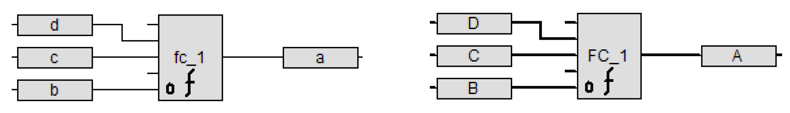
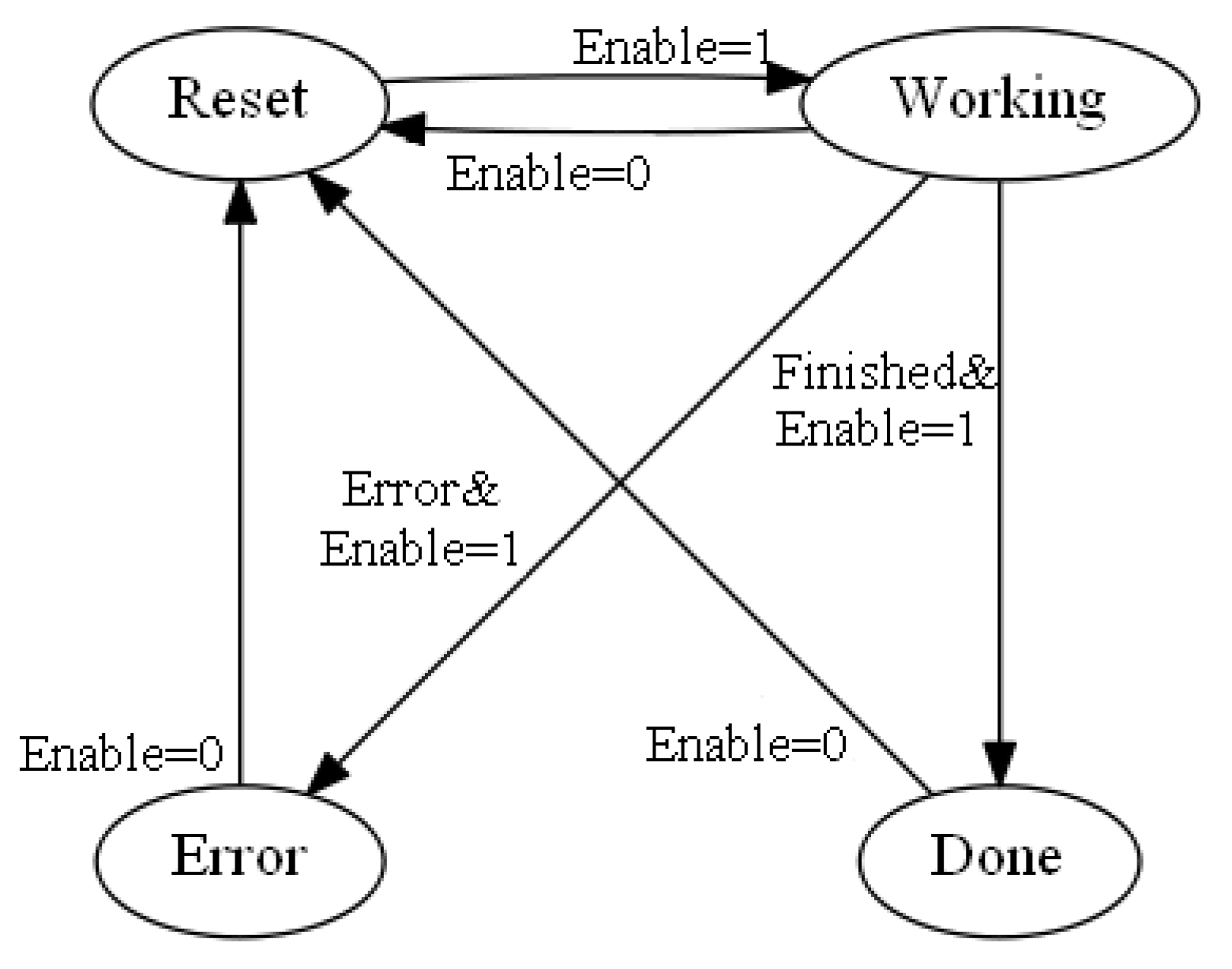
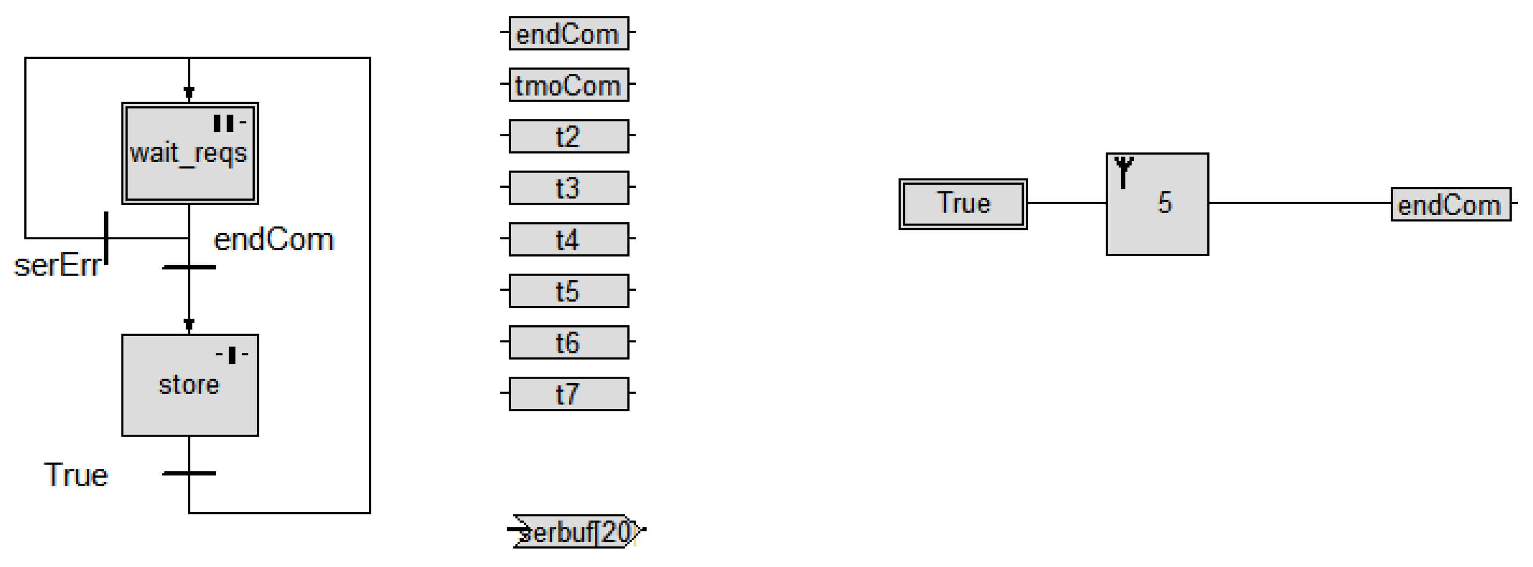
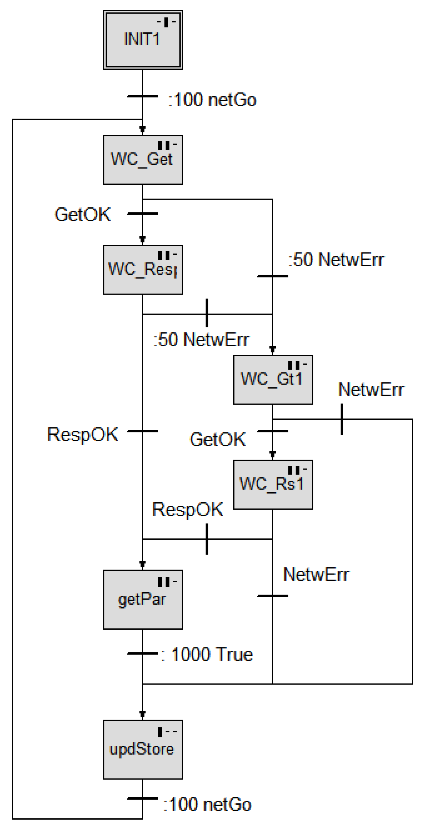
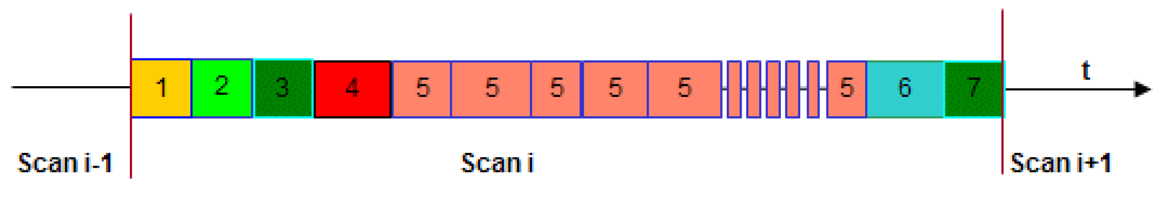
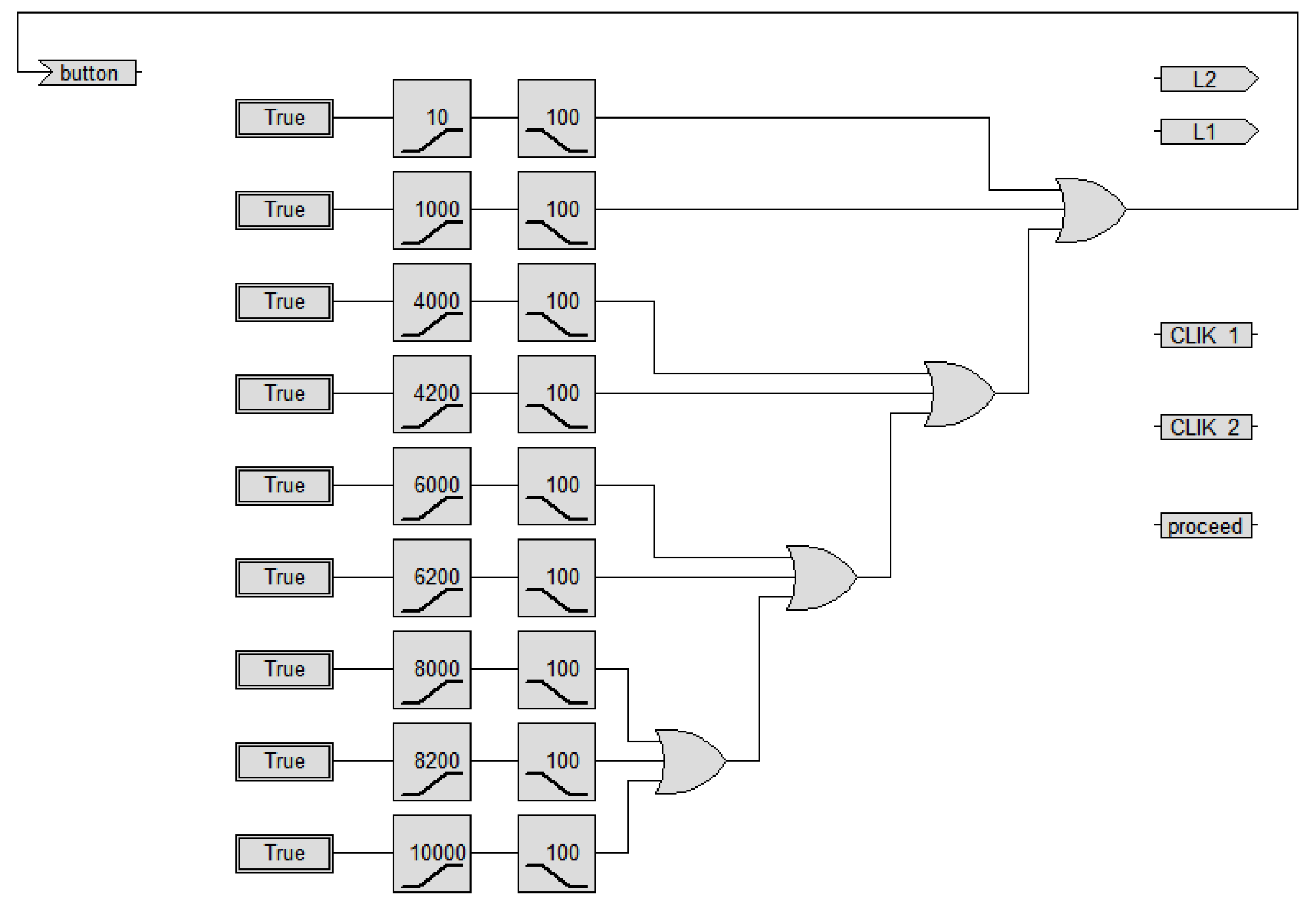
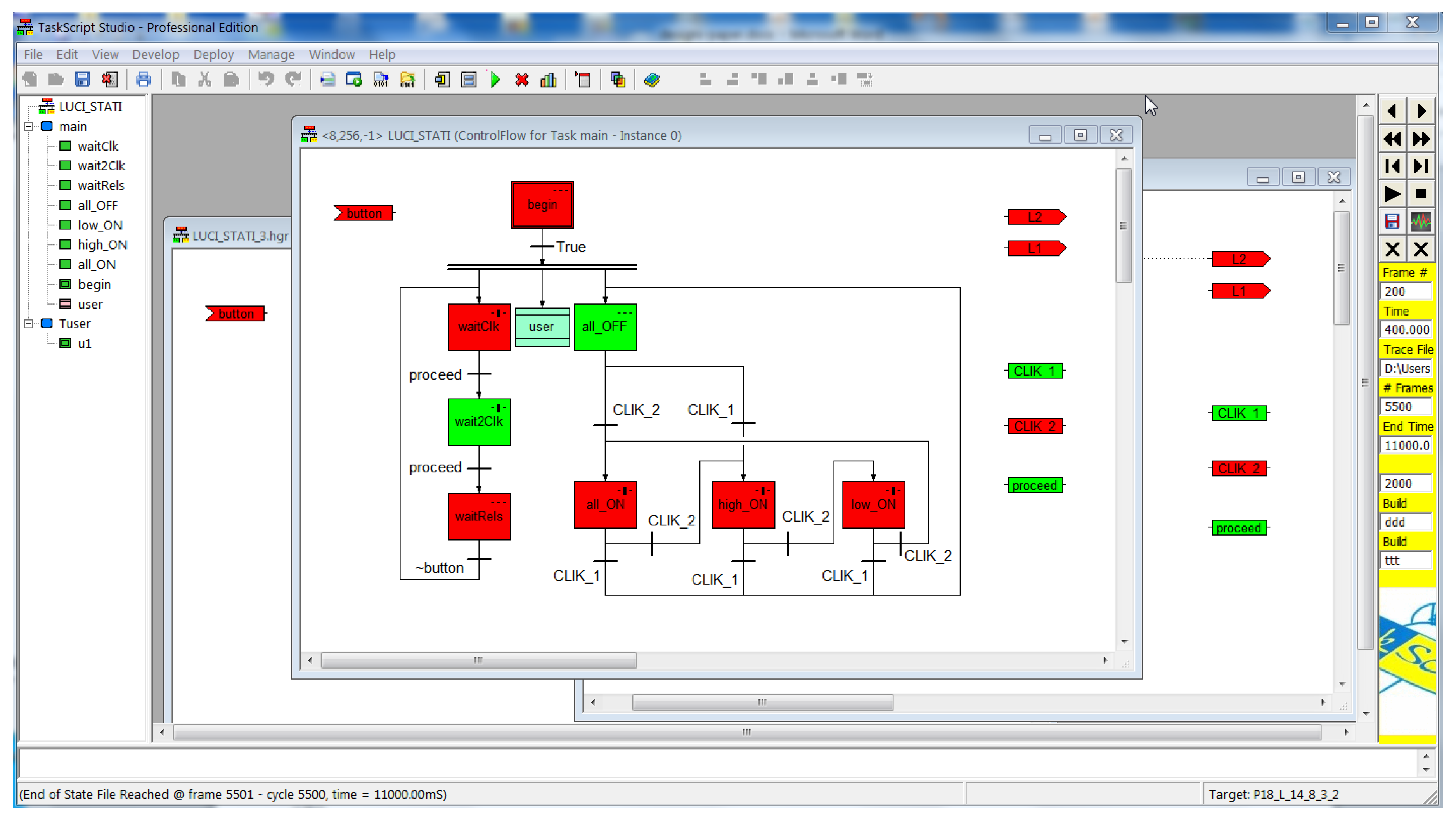
Table 1.
Primitive Operator groups.
| Group | Result Type | Source Type | Other Source Type | Notes |
|---|---|---|---|---|
| Logic | Bit/Word | Bit/Word | ||
| Arithmetic | Word | Word | ||
| Shift/Rotate | Word | Word | ||
| Compare | Word | Bit | ||
| Choice | Bit/Word | Bit/Word | Bit (selector) | |
| Composition | Word | Bit | ||
| Extraction | Bit | Word | Word (selector) | |
| Array Subscripting | Bit/Word | Bit/Word | Word (subscript) | |
| Extrn. Function | Bit/Word | Bit/Word | ||
| Edge | Bit | Bit | ||
| Delay | Bit | Bit | Stateful | |
| Counter | Bit | Bit | Bit (count) | Stateful |
| Communicators | Bit | Bit | Word (buf length) | Stateful |
Table 2.
Model-level characteristics of the different CPSs.
| Model features | Lights | TransfertMon | EnergyGateway | LithyumBMS |
|---|---|---|---|---|
| # Tasks | 2 | 4 | 5 | 6 |
| # Steps | 8 | 23 | 44 | 42 |
| # parallel threads | 2 | 5 | 11 | 5 |
| # discrete I/O | 3 | 23 | 8 | 12 dig + 2 anlg |
| # serial ports | 0 | 0 | 0 | 1 SPI + 1 UART |
| # of network ports | 0 | 1 | 1 | 1 |
| # of protocols | 0 | 1 | 1 | 2 |
| # internal variables | 3 | 22 | 40 | 25 |
Table 3.
Controller Performance for the different CPSs.
| Controller Performance | Lights-8bit | Lights-16bit | TransfertMon | EnergyGateway | LithyumBMS |
|---|---|---|---|---|---|
| Controller board | P18L_14_8_3_2 | P24_S_8_4_3_3 | P18_E_SP_FTC_485 16_5_2_2 | P18_E_SP_FTC_485 12_13_9_2 | P18_E_SP_FT_485 8_8_10_3 |
| Board size | ~15cm2 | ~15cm2 | ~76cm2 | ~55cm2 | ~76cm2 |
| Controller CPU | PIC18F25K22 | TS-P24EP-GP202 | PIC18F87J60 | PIC18F87J60 | PIC18F87J60 |
| CPU Clock | 64MHz | 140MHz | ~42MHz | ~42MHz | ~42MHz |
| CPU bits | 8 | 16 | 8 | 8 | 8 |
| Controller Power | <50mW | <0.2W | <2W | <1W | <2W |
| Avg. scan time (ms) | <0.1ms | <15us | <0.2ms | <0.2ms | <0.25ms |
Table 4.
Development effort in person-hours for the different CPSs.
| Development Effort (pers-hrs) | Lights | TransfertMon | EnergyGateway | LithyumBMS |
|---|---|---|---|---|
| modeling of logic | 1 | 4 | 8 | 16 |
| modeling of communication | - | 4 | 4 | 8 |
| domain knowledge | - | 4 | 4 | 16 |
| simulation-debug | 1 | 4 | 8 | 16 |
| physical setup | 1 | 8 | 4 | 16 |
© 2019 by the author. Licensee MDPI, Basel, Switzerland. This article is an open access article distributed under the terms and conditions of the Creative Commons Attribution (CC BY) license (http://creativecommons.org/licenses/by/4.0/).
Share and Cite
MDPI and ACS Style
Manione, R. A full Model-Based Design Environment for the Development of Cyber Physical Systems. Designs 2019, 3, 15. https://doi.org/10.3390/designs3010015
AMA Style
Manione R. A full Model-Based Design Environment for the Development of Cyber Physical Systems. Designs. 2019; 3(1):15. https://doi.org/10.3390/designs3010015
Chicago/Turabian StyleManione, Roberto. 2019. "A full Model-Based Design Environment for the Development of Cyber Physical Systems" Designs 3, no. 1: 15. https://doi.org/10.3390/designs3010015