Probability Study on the Thermal Stress Distribution in Thick HK40 Stainless Steel Pipe Using Finite Element Method

Abstract

The present work deals with the development of a finite element methodology for obtaining the stress distributions in thick cylindrical HK40 stainless steel pipe that carries high-temperature fluids. The material properties and loading were assumed to be random variables. Thermal stresses that are generated along radial, axial, and tangential directions are generally computed using very complex analytical expressions. To circumvent such an issue, probability theory and mathematical statistics have been applied to many engineering problems, which allows determination of the safety both quantitatively and objectively based on the concepts of reliability. Monte Carlo simulation methodology is used to study the probabilistic characteristics of thermal stresses, and was implemented to estimate the probabilistic distributions of stresses against the variations arising due to material properties and load. A 2-D probabilistic finite element code was developed in MATLAB, and the deterministic solution was compared with ABAQUS solutions. The values of stresses obtained from the variation of elastic modulus were found to be low compared to the case where the load alone was varying. The probability of failure of the pipe structure was predicted against the variations in internal pressure and thermal gradient. These finite element framework developments are useful for the life estimation of piping structures in high-temperature applications and for the subsequent quantification of the uncertainties in loading and material properties.

1. Introduction

Axisymmetric pressurized thick cylindrical pipes are widely used in chemical, petroleum, and military industries, in fluid transfer plants and power plants, as well as in nuclear power plants due to ever-increasing industrial demand. These pipes are generally introduced to excessive pressures and temperatures that are either steady or continuous. In general, it is very difficult to exactly estimate the thermal stresses generated on structural components such as thick pipe due to pressure and temperature changes. Therefore, probability theory and mathematical statistics have been applied, which allows the safety to be determined both quantitatively and objectively based on the concepts of reliability. The stress distribution in nuclear power plant piping systems remains a main concern, and deterministic structural integrity assessment needs to be combined with probabilistic approaches in order to consider uncertainties in material and load properties. The deterministic finite element method for a defined problem can be transformed to a probabilistic approach by considering some of the inputs as random variables. The uncertainty associated with the strength prediction can be calculated by simulation techniques such as Monte Carlo simulation, which allow the values for basic stiffness variables to be generated based on their statistical distributions (i.e., probability density functions). A relevant strength variable for pipe is the elastic modulus, and load variables include internal pressure and temperature change. The objective herein was to compile statistical information and data based on literature review regarding both strength and load random variables relevant to thick pipe structure for the quantification of the probabilistic characteristics of these variables. The quantification of random variables of loads and material properties in terms of their means, standard deviations, or coefficients of variation and probability distributions can be achieved by data collection and analysis. The initial step is to gather as much as data in order to consider what is appropriate for the unarranged variables under study. The second step is concerned with the statistical analysis of the data to determine the probabilistic characteristics of these variables.

Zhou and Tu [1] carried out a work to estimate the service life of a high-temperature furnace, which is very difficult due to the variability of creep data. To study the random nature of service life, a new stochastic creep damage model is proposed in their work. A comparison with results calculated using the Monte Carlo method verified the creep damage model. The randomness of the creep damage was demonstrated with a calculation on HK40 furnace tubes, providing an effective means of assessing the reliability of the furnace tubes. In the present work, the material parameters of the HK40 were adapted from Zhou and Tu [1]. SM Rehman et al. [2] investigated the natural frequencies and bulking loads for cylindrical shells with and without cracks. Chanylew Taye and Alem Bazezew [3] studied the creep analysis of boiler tubes by finite element method. In their work, an analysis is developed for the determination of the creep deformation of an axisymmetric boiler tube subjected to axisymmetric loads.

Heat flux determination finds it application in the field of materials processing [4,5,6]. Holm Altenbach et al. [7] presented a creep model to reflect the basis features of creep in structures including the evaluation of inelastic deformations, relaxation and redistribution of stresses, as well as the local reduction of material strength. The solutions were compared with the finite element solutions of ANSYS and ABAQUS finite element codes with user creep model subroutines. The geometric parameters and loading conditions for the present work were adopted from Holm Altenbach [7]. Finally, Oliver C. Ibe [8] presented a study of the fundamentals of applied probability and random processes. The present work follows the probabilistic equations, and a comprehensive review on the contour method has already been carried out by Prime and DeWald [8]. Node correction in a control volume mesh is not possible because the mesh needs to be regular. That weakness is not present in the finite element based finite volume method (FEMFVM).

The stress induced by thermal gradient through the wall is given by [9]:

$${\sigma }_r^T\left(\mathrm{Radial}\mathrm{stress}\right)=\frac{E\alpha \left(\mathsf{\Delta }T\right)}{2\left(1-\mu \right)\ln a} \left[-2\ln \left(\frac{r_0}{r}\right)+\frac{{\left(\frac{r_0}{r}\right)}^2-1}{a^2-1}\ln a\right],$$

(1)

$${\sigma }_{\theta }^T(\mathrm{Circumferential}\mathrm{stress})=\frac{E\alpha \left(\mathsf{\Delta }T\right)}{2\left(1-\mu \right)\ln a} \left[1-\ln \left(\frac{r_0}{r}\right)-\frac{{\left(\frac{r_0}{r}\right)}^2+1}{a^2-1}\ln a\right],$$

(2)

$${\sigma }_z^T\left(\mathrm{Axial}\mathrm{stress}\right)=\frac{E\alpha \left(\mathsf{\Delta }T\right)}{2\left(1-\mu \right)\ln a} \left[1-2\ln \left(\frac{r_0}{r}\right)-\frac{2\ln a}{a^2-1}\right],$$

(3)

$$\begin{gathered} {\sigma }_r^T\left(\mathrm{Radial}\mathrm{stress}\right)=\frac{E\alpha \left(\mathsf{\Delta }T\right)}{2\left(1-\mu \right)\ln a}\left[-2\ln \left(\frac{r_0}{r}\right)+\frac{{\left(\frac{r_0}{r}\right)}^2-1}{a^2-1}\ln a\right] \\ {\sigma }_{\theta }^T=\frac{E\alpha \left(\mathsf{\Delta }T\right)}{2\left(1-\mu \right)\ln a}\left[1-\ln \left(\frac{r_0}{r}\right)-\frac{{\left(\frac{r_0}{r}\right)}^2+1}{a^2-1}\ln a\right], \end{gathered}$$

(4)

$${\sigma }_z^T\left(\mathrm{Axial}\mathrm{stress}\right)=\frac{E\alpha \left(\mathsf{\Delta }T\right)}{2\left(1-\mu \right)\ln a}\left[1-2\ln \left(\frac{r_0}{r}\right)-\frac{2\ln a}{a^2-1}\right].$$

(5)

2. Analytical Solution

The Stresses for Thick-Walled Cylinder Pipe under Internal Pressure (P) and Thermal Gradient ($\Delta T$)

Radial stress is given by [10]:

$${\sigma }_r={\sigma }_r^P+{\sigma }_r^T,$$

(6)

$${\sigma }_r= \frac{P}{a^2-1}\left[1-{\left(\frac{r_0}{r}\right)}^2\right]+\frac{E\alpha \left(\mathsf{\Delta }T\right)}{2\left(1-\mu \right)\ln a} \left[-2\ln \left(\frac{r_0}{r}\right)+\frac{{\left(\frac{r_0}{r}\right)}^2-1}{a^2-1}\ln a\right],$$

(7)

$${\sigma }_r=\frac{P}{a^2-1}\left[1{\left(\frac{r_0}{r}\right)}^2\right]+\frac{E\alpha \left(\mathsf{\Delta }T\right)}{2\left(1-\mu \right)\ln a}\left[-2\ln \left(\frac{r_0}{r}\right)+\frac{{\left(\frac{r_0}{r}\right)}^2-1}{a^2-1}\ln a\right].$$

(8)

Circumferential stress is given by:

$${\sigma }_{\theta }={\sigma }_{\theta }^P+{\sigma }_{\theta }^T,$$

(9)

$${\sigma }_{\theta }= \frac{P}{a^2-1}\left[1+{\left(\frac{r_0}{r}\right)}^2\right]+\frac{E\alpha \left(\mathsf{\Delta }T\right)}{2\left(1-\mu \right)\ln a} \left[1-\ln \left(\frac{r_0}{r}\right)-\frac{{\left(\frac{r_0}{r}\right)}^2+1}{a^2-1}\ln a\right].$$

(10)

Axial stress is given by:

$${\sigma }_z={\sigma }_z^P+{\sigma }_z^T,$$

(11)

$${\sigma }_z= \frac{P}{a^2-1}2\mu +\frac{E\alpha \left(\mathsf{\Delta }T\right)}{2\left(1-\mu \right)\ln a} \left[1-2\ln \left(\frac{r_0}{r}\right)-\frac{2\ln a}{a^2-1}\right].$$

(12)

Finally, von Mises stress is given by:

$${\sigma }_e=\frac{1}{\sqrt{2}}\sqrt{{\left({\sigma }_r-{\sigma }_{\theta }\right)}^2+{\left({\sigma }_{\theta }-{\sigma }_z\right)}^2+{\left({\sigma }_z-{\sigma }_{\theta }\right)}^2},$$

(13)

where ${\sigma }_{\theta }^P$ is the hoop stress induced by pressure (MPa); ${\sigma }_z^P$ is the axial stress induced by pressure (MPa); ${\sigma }_r^P$ is the radial stress induced by pressure (MPa); P is the pressure in (MPa); $r_0$ is the outer radius (mm); and $r_i$ is the inner radius (mm); a is the ratio of outer to inner radius:

$$a= r_0/r_i,$$

(14)

r is the radius at any position of the tube wall (mm); and $\mu$ is Poisson’s ratio. ${\sigma }_{\theta }^T$ is the hoop stress induced by thermal stress (MPa); ${\sigma }_z^T$ is the axial stress induced by thermal stress (MPa); ${\sigma }_r^T$ is the radial stress induced by thermal stress (MPa); E is the elastic modulus of the material (MPa); $\alpha$ is the thermal expansion coefficient of the material ($1/°\mathrm{C}$); $\mathsf{\Delta }T$ is the thermal gradient of the outer wall, and the inner wall temperature is:

$$\Delta T=T_i-T_0.$$

(15)

A thick-walled cylinder pipe carrying high-temperature liquid is considered. The fluid inside the pipe was assumed to completely fill the pipe and exert a constant pressure P. The analysis was carried out in the 2-D plane of the cross section of the pipe (see Figure 1).

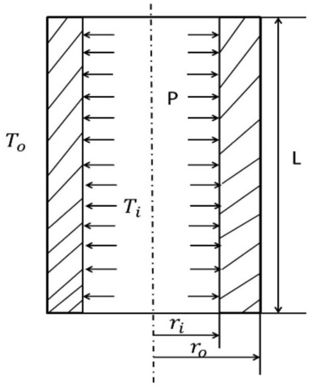
Figure 1. Schematic diagram of the axisymmetric pipe section.

The pipe was made up of material HK40 as per Zhou and Tu [1]. It was stressed to a pressure of 40 MPa. The temperature of the fluid flowing inside the pipe $T_i$ was 500 °C, and the outside temperature $T_0$ was 420 °C (i.e., the pipe was subjected to a thermal gradient $\Delta T$ of 80 °C [11].

The dimensions of the thick pipe section were taken as L of 100 mm, $r_i$ of 25 mm, and $r_0$ of 50 mm. The material properties of HK40 are given as follows: elastic modulus $E \mathrm{of} 1.38\times {10}^5$ Pa, Poisson’s ratio $\mu$ of 0.313, thermal expansion coefficient $\alpha \mathrm{of}1.5\times {10}^{-5}\left(1/°\mathrm{C}\right)$. The obtained values of the radial stress, circumferential stress, axial stress, and von Mises stress are shown in Table 1. Graphs of different stresses vs. radius are shown in Figure 2 and Figure 3.

Table 1. Analytical results of the pipe.

Radius (mm)	Radial Stress (σr) (MPa)	Circumferential Stress (σθ) (MPa)	Axial Stress (σz) (MPa)	Von Mises Stress (σv) (MPa)
26.25	−35.04	61.70	8.34	83.93
28.75	−26.99	53.66	8.34	70.02
31.25	−20.80	47.46	8.34	59.33
33.75	−15.93	42.59	8.34	50.93
36.25	−12.03	38.70	8.34	44.21
38.75	−8.86	35.53	8.34	38.77
41.25	−6.25	32.92	8.34	34.29
43.75	−4.08	30.74	8.34	30.57
46.25	−2.24	28.91	8.34	27.44
48.75	−0.69	27.35	8.34	24.80

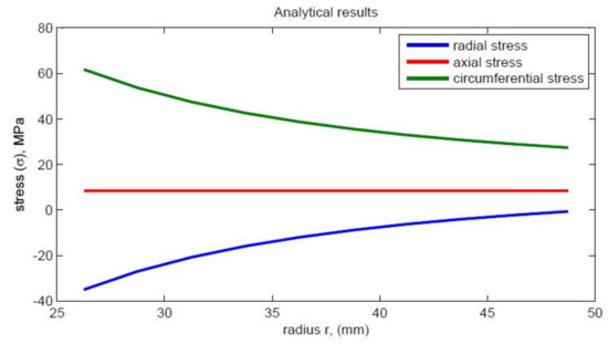
Figure 2. Variation of radial, circumferential, and axial stresses.

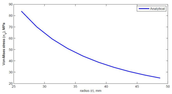
Figure 3. Von Mises stress vs. radius.

3. Axisymmetric Finite Element Analysis Using ABAQUS Software

A pipe made up of HK40 material was considered with a pipe length L of 100 mm, inner radius r_i of 25 mm, and outer radius r₀ of 50 mm. The material properties are elastic modulus (E) of 1.38 × 10⁵ MPa, Poisson’s ratio µ of 0.313, coefficient of thermal expansion (α) of 1.5 × 10⁻⁵ (1/°C). The model was meshed with element type CAX4R, a four-noded bilinear quadrilateral element, and the mesh grid was 10 × 10 elements and was fixed in the axial direction U2 of 0, as shown in Figure 4. The loading conditions were internal pressure P = 40 MPa, inside temperature $T_i$ of 500 °C, outside temperature $T_0$ of 420 °C, thermal gradient $\Delta T$ of 80 °C. Figure 4 shows the model with meshing and applied boundary conditions in ABAQUS. Analysis on the sweep of different stress elements before and after analysis is shown in Figure 5, Figure 6, Figure 7 and Figure 8 below, along with comparisons of various stresses which are shown in Figure 9, Figure 10 and Figure 11. Table 2 and Table 3 show the comparisons of analytical and finite element analysis (FEA) using ABAQUS results by using von Mises stress.

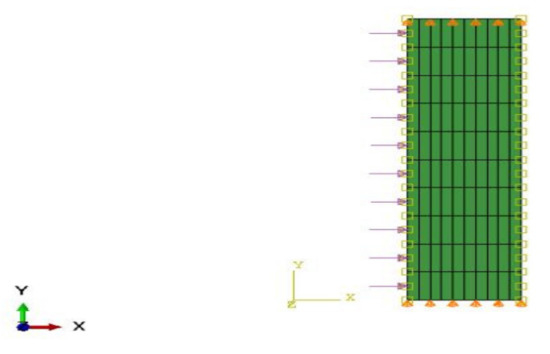
Figure 4. Meshing, boundary conditions, internal pressure, and thermal gradient of axisymmetric thick pipe.

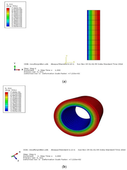
Figure 5. Analysis on sweep of radial stress elements: (a) before, (b) after.

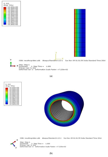
Figure 6. Analysis on sweep of axial stress elements: (a) before, (b) after.

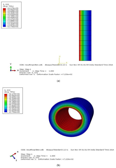
Figure 7. Analysis on sweep of circumferential stress elements: (a) before, (b) after.

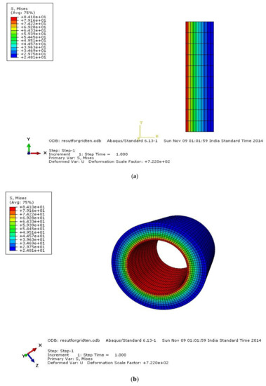
Figure 8. Analysis on sweep of von Mises stress elements: (a) before, (b) after.

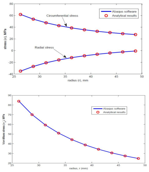
Figure 9. Radial and circumferential stress and von Mises stress.

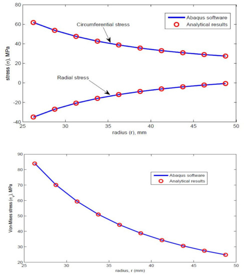
Figure 10. Radial and circumferential stress, and von Mises stress.

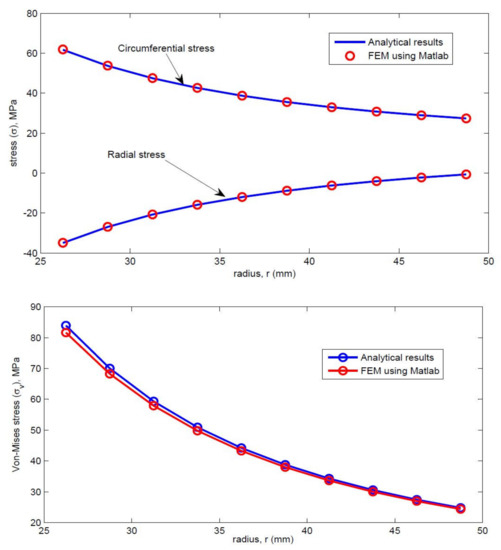
Figure 11. Radial and circumferential stress, and von Mises stress.

Table 2. Comparison of analytical and finite element analysis (FEA) using ABAQUS results by using von Mises stress.

Radius (mm)	Analytical Results			FEA Using ABAQUS
	${\mathit{\sigma }}_{\mathit{r}} \left(\mathbf{MPa}\right)$	${\mathit{\sigma }}_{\mathit{\theta } }\left(\mathbf{MPa}\right)$	${\mathit{\sigma }}_{\mathit{V}} \left(\mathbf{MPa}\right)$	${\mathit{\sigma }}_{\mathit{r}} \left(\mathbf{MPa}\right)$	${\mathit{\sigma }}_{\mathit{\theta }} \left(\mathbf{MPa}\right)$	${\mathit{\sigma }}_{\mathit{V}} \left(\mathbf{MPa}\right)$
26.2500	−35.0416	61.7082	83.9361	−35.1470	61.7910	84.0936
28.7500	−26.9943	53.6610	70.0273	−27.0669	53.7178	70.1337
31.2500	−20.8000	47.4667	59.3306	−20.8515	47.5068	59.4038
33.7500	−15.9305	42.5972	50.9312	−15.9679	42.6262	50.9821
36.2500	−12.0333	38.7000	44.2184	−12.0611	38.7214	44.2537
38.7500	−8.8658	35.5324	38.7720	−8.8868	35.5485	38.7961
41.2500	−6.2565	32.9232	34.2951	−6.2727	32.9354	34.3109
43.7500	−4.0816	30.7483	30.5730	−4.0942	30.7578	30.5825
46.2500	−2.2498	28.9165	27.4476	−2.2597	28.9239	27.4520
48.7500	−0.6925	27.3592	24.8000	−0.7004	27.3650	24.8004

Table 3. Comparison of analytical and FEM using MATLAB results.

Radius (mm)	Analytical Results			FEM Using MATLAB
	${\mathit{\sigma }}_{\mathit{r}} \left(\mathbf{MPa}\right)$	${\mathit{\sigma }}_{\mathit{\theta }} \left(\mathbf{MPa}\right)$	${\mathit{\sigma }}_{\mathit{V}} \left(\mathbf{MPa}\right)$	${\mathit{\sigma }}_{\mathit{r}} \left(\mathbf{MPa}\right)$	${\mathit{\sigma }}_{\mathit{\theta }} \left(\mathbf{MPa}\right)$	${\mathit{\sigma }}_{\mathit{V}} \left(\mathbf{MPa}\right)$
26.250	−35.041	61.708	83.936	−34.950	61.883	81.636
28.750	−26.994	53.661	70.027	−26.926	53.768	68.244
31.250	−20.800	47.466	59.330	−20.748	47.532	57.917
33.750	−15.930	42.597	50.931	−15.890	42.635	49.789
36.250	−12.033	38.700	44.218	−12.002	38.720	43.280
38.750	−8.865	35.532	38.772	−8.841	35.540	37.990
41.250	−6.256	32.923	34.295	−6.237	32.923	33.636
43.750	−4.081	30.748	30.573	−4.067	30.742	30.010
46.250	−2.249	28.916	27.447	−2.238	28.906	26.963
48.750	−0.692	27.359	24.800	−0.684	27.346	24.378

3.1. Comparison of Analytical and FEA using ABAQUS

Several examples were solved to show the accuracy of the analyticalsolution in comparison with the FEA analysis. Both stress distributions such as the circumferential and radial stresses were obtained.Circumferential stress gradually decreases and radial stress, von mises increases as shown in the Figure 9.

3.2. Comparison of Analytical Results and FEA Results Using Abaqus and FEM Using MATLAB

Several examples were solved to show the accuracy of the analyticalsolution in comparison with the FEA usign MATLAB analysis. Both stress distributions such as the circumferential and radial stresses were obtained.Circumferential stress gradually decreases and radial stress, von mises increases as shown in the Figure 10.

4. Probabilistic Study

4.1. Monte Carlo Simulation

The Monte Carlo method involves randomly sampling the distributed input variables many times so as to build a statistical picture of the output quantities. This method has a wide range of applicability, with engineering applications being only one. The Monte Carlo method is particularly appropriate when there is a large number of independent variables that can influence the outcome. The Monte Carlo method is being used increasingly in structural integrity applications. The probabilistic simulation uses a Monte Carlo method with Latin hypercube sampling [12]. This is an efficient technique that permits a large number of distributed variables to be addressed. Each variable takes a finite number of values, each representing a range of values (i.e., a “bin”). All bins are of equal probability. The Latin hypercube algorithm ensures that all variable bins are sampled in the minimum number of trails (though not, of course, in all possible combinations). Moreover, because all bins are of equal probability, it follows that all trails are of equal probability, thus ensuring that all trails are of equal weight in the simulation [13].

4.2. Distributed Structural Parameters

The parameters that are required to calculate thermal stresses and which are taken as distributed in simulations are: elastic modulus, internal pressure, and temperature change. Normal distributions were used for stresses and lognormal distribution was used for material properties.

4.3. Lognormal Distribution

A random variable X is considered to have a lognormal distribution if Y = ln(X) has a normal probability distribution. The density function of the lognormal distribution is given by:

$$f_X\left(x\right)= \frac{1}{x\sigma \sqrt{2\pi }}exp\left[-\frac{1}{2}{\left(\frac{\ln x-\mu }{\sigma }\right)}^2\right], 0<x<\infty .$$

(16)

The notations X$~LN\left(\mu ,{\sigma }^2\right)$ provide an abbreviated description of a lognormal distribution. The notation states that X is log-normally distributed with mean $\mu$ and variance ${\sigma }^2$.

4.4. Input Distribution

4.4.1. Due to Variability in Material Property

The lognormal distribution for the Young’s modulus of elasticity ($E$) is:

$$f_X\left(E;\mu ,\sigma \right)= \frac{1}{x{\sigma }_x\sqrt{2\pi }}exp\left[-\frac{1}{2}{\left(\frac{\ln x-{\mu }_x}{{\sigma }_x}\right)}^2\right].$$

(17)

Lognormal distribution for E = 1.38 × 10⁵ Pa.

Monte Carlo simulations (MCSs) N = 1000 runs were carried out to estimate the stress distribution for the number of elements in the radial direction.

$$\mathrm{Coefficient}\mathrm{of}\mathrm{variance}=0.2=\frac{\sigma }{\mu }=\frac{\sigma }{E},$$

(18)

$$\mathrm{Mean}=({\mu }_x)= \log \frac{{\mu }^2}{\sqrt{{\sigma }^2+{\mu }^2}},$$

(19)

$$\mathrm{Standard}\mathrm{deviation}=\left({\sigma }_x\right)=\sqrt{\log \frac{{\sigma }^2}{{\mu }^2+1}}.$$

(20)

The elastic modulus was lognormally distributed with standard deviation as 1.38 × 10⁵ Pa. Figure 12 represents Young’s modulus due to the variation of the material properties.

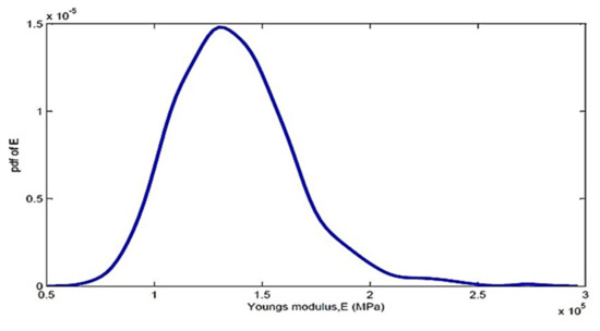
Figure 12. Young’s modulus due to the variation of the material properties.

4.4.2. Due to Load Variability

Normal Distribution

This distribution is the basis for many statistical methods. The normal density function for a random variable X is given by:

$${\mathrm{f}}_{\mathrm{X}}\left(\mathrm{x}\right)=\frac{1}{\mathsf{\sigma }\sqrt{2\mathsf{\pi }}}\exp \left[-\frac{{\left(\mathrm{x}-\mathsf{\mu }\right)}^2}{2{\mathsf{\sigma }}^2}\right],-\infty <\mathrm{x}<\infty .$$

(21)

It is common to use the notation X$~N\left(\mu ,{\sigma }^2\right)$ to provide an abbreviated description of a normal distribution. The notation states that X is normally distributed with mean $\mu$ and variance ${\sigma }^2$.

In this study, $P$ and $\Delta T$ are random variables in r-radial and z-axial directions. The normal distribution is of the form:

$${\mathrm{f}}_{\mathrm{X}}\left(\mathrm{x};\mathsf{\mu },\mathsf{\sigma }\right)={\mathrm{f}}_{\mathrm{X}}\left(\mathrm{P},\Delta \mathrm{T};\mathsf{\mu },\mathsf{\sigma }\right)=\frac{1}{\mathsf{\sigma }\sqrt{2\mathsf{\pi }}}\exp \left[-\frac{{\left(\mathrm{x}-\mathsf{\mu }\right)}^2}{2{\mathsf{\sigma }}^2}\right],\mathrm{where}-\infty <\mathrm{x}<\infty .$$

(22)

Normal Distribution for Pressure

Mean = $P$, variance = ${\sigma }^2$, coefficient of variance = 0.1 = $\frac{\sigma }{\mu }=\frac{\sigma }{P}$, standard deviation = $\left({\sigma }_x\right)$ = $\sqrt{V}$, pressure ($P$) = $x*{\sigma }_x+\mu$.

Pressure was normally distributed with mean and standard deviation of 40 and 4, respectively. The nominal distribution of pressure is represented in Figure 13 below.

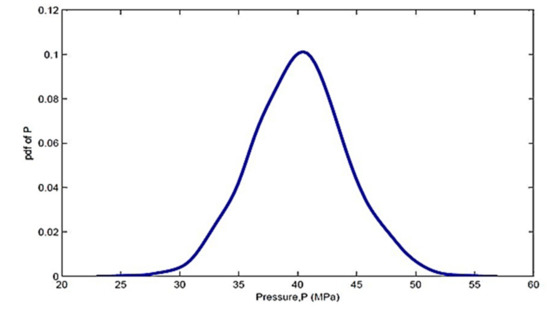
Figure 13. Nominal distribution of pressure.

Normal distribution for thermal gradient $\Delta T$:

$$\mathrm{Mean}= \Delta T={\mathrm{T}}_{\mathrm{i}\left(\mathrm{x}\right)}-{\mathrm{T}}_0=\frac{\mathsf{\sigma }}{\mathsf{\mu }}=\frac{\mathsf{\sigma }}{\Delta T=({\mathrm{T}}_{\mathrm{i}\left(\mathrm{x}\right)}-{\mathrm{T}}_0)},$$

(23)

$$\mathrm{Standard}\mathrm{deviation}=\left({\mathsf{\sigma }}_{\mathrm{x}}\right)=\sqrt{\mathrm{V}},$$

(24)

$$\mathrm{Thermal}\mathrm{gradient}(\Delta T)={\mathrm{x}*\mathsf{\sigma }}_{\mathrm{x}}+\mathsf{\mu }.$$

(25)

Variance = ${\sigma }^2$, coefficient of variance = 0.05, inside temperature was varying and outside temperature was kept constant, and thermal gradient was normally distributed with mean and standard deviation of 80 and 4, respectively. The nominal distribution of the thermal gradient is represented in Figure 14 below.

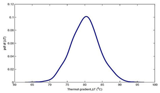
Figure 14. Nominal distribution of thermal gradient.

5. Probabilistic Finite Element Formulation

The development of a probabilistic finite element formulation for the axisymmetric pipe section was based on an available procedure for determining the finite element analysis of an axisymmetric pipe section. The axisymmetric section of the pipe used for finite element analysis was discretized into ten finite elements in the radial direction and 10 elements in the axial direction, and the geometry of the FE mesh is shown in Figure 15 below.

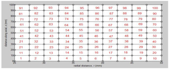
Figure 15. Finite element mesh for the geometry of an axisymmetric pipe section.

The constitutive equation for the axisymmetric pipe is given by:

$$\sigma =C\left(\in -{\in }_0\right),$$

(26)

where σ is the resultant stress vector induced due to the combined effect of pressure and temperature gradient. The components of stress and strain vector are represented as:

$$\begin{gathered} \sigma ={\left({\mathsf{\sigma }}_{\mathrm{r}}{\mathsf{\sigma }}_{\mathrm{z}}{\mathsf{\sigma }}_{\mathsf{\theta }}{\mathsf{\tau }}_{\mathrm{rz}}\right)}^{\mathrm{T}}, \\ \in ={\left({\in }_{\mathrm{r}}{\in }_{\mathrm{z}}{\in }_{\mathsf{\theta }}{\mathsf{\gamma }}_{\mathrm{rz}}\right)}^{\mathrm{T}}, \\ {\in }_0=\left(\mathsf{\alpha }\Delta T\left(\mathrm{r},\mathrm{z}\right)\mathsf{\alpha }\Delta T\left(\mathrm{r},\mathrm{z}\right)\mathsf{\alpha }\Delta T\left(\mathrm{r},\mathrm{z}\right)0\right). \end{gathered}$$

(27)

${\in }_0$ is the initial strain vector due to temperature change, α is the coefficient of linear expansion, and the superscript “T” is the transpose operator. C is the constitutive matrix which is a function of E, the Young’s modulus of elasticity of the isotropic material, and μ is Poisson’s ratio. E is considered to be a random variable, and is of the form:

$$E=E\left(\mathrm{x}\right)=\mathrm{LN}\left(\mathsf{\mu },{\mathsf{\sigma }}^2\right).$$

(28)

Therefore, the material matrix can be expressed as:

$$C\left(\mathrm{r},\mathrm{z}\right)=\frac{\mathrm{E}\left(\mathrm{r},\mathrm{z}\right)}{\left(1-2\vartheta \right)\left(1+\vartheta \right)}(\begin{array}{cccc}1-\vartheta & \vartheta & \vartheta & 0\\ \vartheta & 1-\vartheta & \vartheta & 0\\ \vartheta & \vartheta & 1-\vartheta & 0\\ 0& 0& 0& \frac{1-2\vartheta }{2}\end{array}).$$

(29)

6. Derivation of Stiffness Matrix

In the next process, the four-noded finite element quadrilateral element for axisymmetric probabilistic finite element analysis with two degrees per node is denoted by $\delta \left[u,w\right]$, where $u\left(r,z\right)$ is the vector of radial displacement and $w\left(r,z\right)$ is the vector of axial displacement. Since it is the axisymmetric case, displacement in the $\theta$ direction is zero. The internal strain energy, U, can be written as:

$$U= \frac{1}{2}{\delta }_e^T{K}_e{\delta }_e,$$

(30)

where ${\delta }_e$ is the element displacement vector and $K_e$ is the element stiffness matrix of the pipe section, expressed as:

$$K_e\left(r,z\right)={{\displaystyle \int }}_{r1}^{r_2}{{\displaystyle \int }}_{z_1}^{z_2}\left[BC\left(r,z\right)B^T\right]2\pi r dr dz.$$

(31)

B are the strain-displacement transfer matrices (derivatives of FE shape functions) and are independent of material properties. The limits $r_1$ and $r_2$ are the inner and outer radii of the cylindrical pipe, and $L$ is the length of pipe from $z_1$ to $z_2$. C is considered to be a random variable.

The element load matrix is given by:

$$F_e\left(r,z\right)={{\displaystyle \int }}_{r1}^{r_2}{{\displaystyle \int }}_{z_1}^{z_2}\left[BC\left(r,z\right){\in }_o\right]2\pi r dr dz.$$

(32)

A Gauss quadrature integration scheme is used to evaluate the above integrals. The global stiffness matrix $K$ is obtained by assembling all the element stiffness matrices $K_e$. Subsequently, the nodal displacements are estimated by solving the finite element governing equation.

The global load vector $F$ and the displacement vector obtained from this governing equation are used for calculating the strains of each element at the centroid location.

$$\left[K\left(\omega \right)\right] \left[\delta \left(\omega \right)\right]=F\left(\omega \right),$$

(33)

where $\omega$ is a random variable. So, Monte Carlo simulations were used to simulate the stresses for each element. Finally, the stress contours for each element in the radial direction were obtained.

Material Specifications

The pipe was made up of material HK40. It was stressed to a pressure P of 40 MPa and subjected to a thermal gradient ΔT of 80 °C. The dimensions of the thick pipe section were L of 100 mm, r_i of 25 mm, and r₀ of 50 mm, respectively. The material properties of HK40 are given as follows: elastic modulus (E) of 1.38 × 10⁵ Pa, Poisson’s ratio (µ) of 0.313, thermal expansion coefficient (α) of 1.5 × 10⁵ (1/°C). For the numerical calculations, the random variable for Young’s modulus of elasticity is $E$.

7. Probabilistic Study: Output Distribution

The output distribution is a complete and systematic framework for the probabilistic modeling of expected material variability and load fluctuations for the fatigue design.

7.1. Output Distribution Due to Material Variability

In order to characterize the material variability on the cyclic stress–strain and strain–life responses of the various elements under multi-axial fatigue, the various random variables were calculated. A comparison of various stresses is shown in Figure 16, Figure 17, Figure 18 and Figure 19.

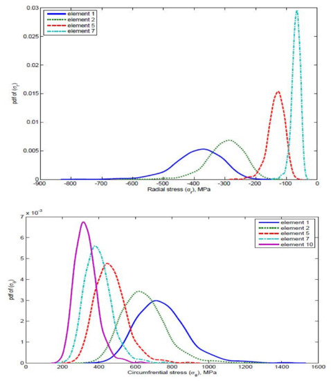
Figure 16. Comparison of radial stress and circumferential stress for different elements where $E$ is a random variable.

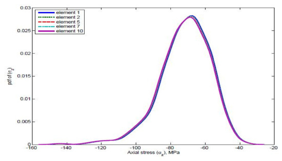
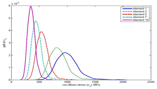
Figure 17. Comparison of axial stress and von Mises stress for different elements when E is a random variable.

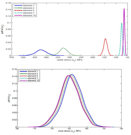
Figure 18. Comparison of radial stress and axial stress for different elements when $E,P, \mathrm{and} \Delta T$ are random variables.

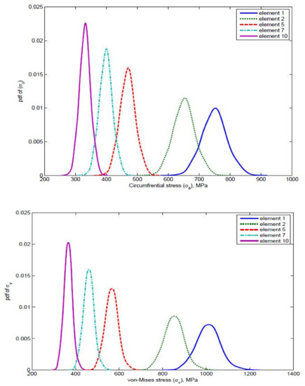
Figure 19. Comparison of circumferential stress and von Mises stress for different elements when $E,P,\mathrm{and}\Delta T$ are random variables.

7.2. Output Distribution Due to Both Material and Load Variability

The Figure 18 and Figure 19 below show the Output Distribution Due to Both Material and Load Variability with each different element. In each graph element 10 has the highest amount of stress when compared to other elements.

8. Probability of Failure of Von Mises Stress with Respect to Yield Strength

The difference in the von Mises stress lies in the selection of the shell face being either positive or negative, commonly known as SPOS and SNEG in ABAQUS [14].

Probability of failure:

$$P_F=P[{\sigma }_V>S_Y\left]=1-P\right[{\sigma }_{V }\le S_Y].$$

(34)

Yield strength $({\sigma }_Y)$ = 241 MPa for HK40 (austenitic heat-resistant stainless steel) material. Probability in the failure of von Mises stress is represented in Figure 20 below.

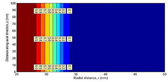
Figure 20. Probability in failure of von Mises stress.

9. Stress Contours

The contour method was used to measure the stress in the component normal to the section surface for both left and right sides, as shown in Figure 21, Figure 22, Figure 23 and Figure 24. Generally, in the contour method, we can study the numerical data in order to verify that it could accurately measure various types of stresses. In our study, we measured various stresses (i.e., radial, circumferential, axial, von Mises) of the HK40 material.

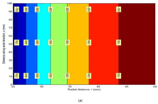
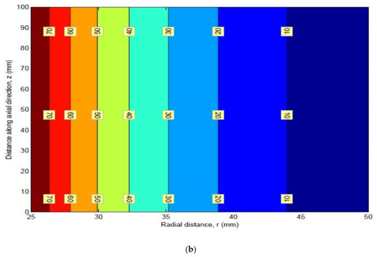
Figure 21. (a) Mean and (b) standard deviation of radial stress.

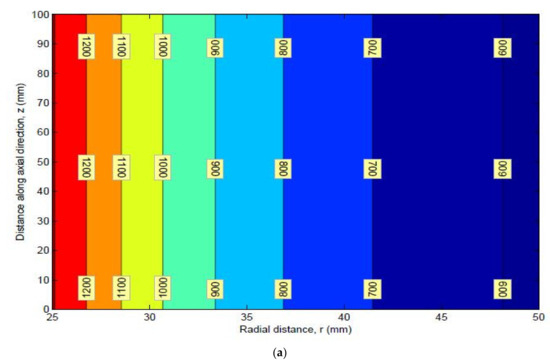
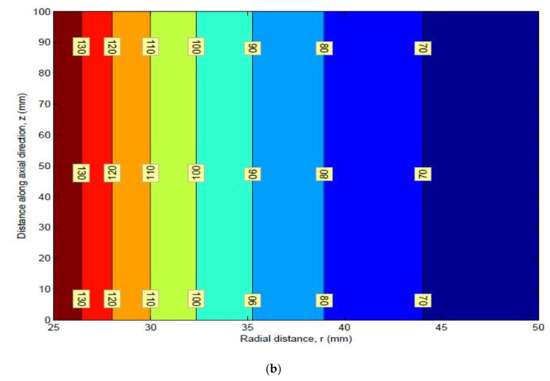
Figure 22. (a) Mean and (b) standard deviation of circumferential stress.

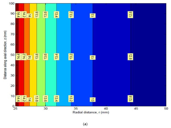
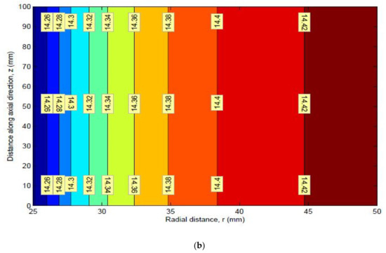
Figure 23. (a) Mean and (b) standard deviation of axial stress.

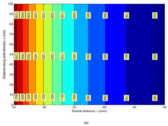
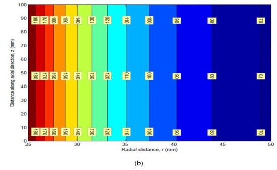
Figure 24. (a) Mean and (b) Standard deviation of Von-Mises stress.

Mean Stress Contours for HK40 Material

In designing for the durability, the presence of direction of axial stress with radial distance can influence fatigue behaviour of materials due to a tensile or compressive normal mean stress as shown in the Figure 21, Figure 22, Figure 23 and Figure 24 below.

10. Conclusions

The results were stated and proved with the help of ABAQUS software and FEM using MATLAB, and a very good match was obtained among all of these findings. The finite element framework was enhanced to find the effects of uncertainties in pipe structure due to material properties and loading. Random variable models were used to model the variabilities in material properties and load by using Monte Carlo simulations. Monte Carlo simulations were used to study the probabilistic characteristics of the stress distribution of the pipe structure. The values of thermal stresses obtained from the variation in material properties (e.g., modulus of elasticity) were found to be low compared to the case where the load alone was varying.

The present methodology was used to estimate the probabilistic distributions of thermal stresses against the variations arising due to material properties as well as variations due to thermal loading. The probability of failure of the pipe structure was predicted against the variations in internal pressure and thermal gradient, and finally the results in the contour method indicated that it could be very similar to the results obtained using the analytical formula, when an asymmetrical cut was made, by averaging the stress components of both sides of the cut. The developed methodology could be helpful for the life assessment of piping structures used for high-temperature practices against creep and fatigue failures in further studies.

References

- Zhou, C.; Tu, S. A Stochastic Computation model for the Creep damage of furnace tube. Int. J. Press. Vessel. Pip. 2001, 78, 617–625. [Google Scholar] [CrossRef]
- Rehman, S.M.; Rao, C.S. Vibration buckling and fracture analysis of a cracked cylindrical shell. Int. J. Des. Eng. 2017, 7, 33–53. [Google Scholar]
- Taye, C. Creep Analysis of boiler tubes by FEM. J. EEA 2005, 22, 1–3. [Google Scholar]
- Chakraborty, S.; Ganguly, S.; Chacko, E.Z.; Ajmani, S.K.; Talukdar, P. Estimation of surface heat flux in continuous casting mould with limited measurement of temperature. Int. J. Therm. Sci. 2017, 118, 435–447. [Google Scholar]
- Guthrie, R.I.L.; Isac, M.; Kim, J.S.; Tavares, R.P. Measurements, simulations and analyses of instantaneous heat fluxes from solidifying steels to the surfaces of twin roll casters and of aluminum to plasma-coated metal substrates. Metall. Mater. Trans. B 2000, 31, 1031–1047. [Google Scholar] [CrossRef]
- Wikstrӧm, P.; Blasiak, W.; Berntsson, F. Estimation of the transient surface temperature and heat flux of a steel slab using an inverse method. Appl. Therm. Eng. 2007, 27, 2463–2472. [Google Scholar] [CrossRef]
- Altenbach, H.; Naumenko, K.; Gorash, Y. Numerical Benchmarks for Creep-Damage Modeling; WILEY-VCH: Berlin, Germany, 2007. [Google Scholar]
- Ibe, O. Fundamentals of Applied probability and Random Processes; Academic Press: Cambridge, MA, USA, 2005. [Google Scholar]
- Prime, M.B.; De Wald, A.T. The contour method. In Practical Residual Stress Measurement Methods; Schajer, G.S., Ed.; John Wiley & Sons, Ltd.: Chichester, UK, 2013. [Google Scholar]
- Yao, X. Non-Linear Finite Element Analysis of Tubular Joints. Ph.D. Thesis, University of Illinois at Urbana-Champaign, Champaign, IL, USA, 1989. [Google Scholar]
- Oclon, P.; Taler, J. Mixed finite volume and finite element formulation: Linear quadraliteral elements. In Encyclopedia of Thermal Stresses; Hetnarski, R., Ed.; Springer: Berlin, Germany, 20 Circumferential; pp. 3086–3095.
- Ghasemi, A.R.; Kazemian, A.; Moradi, M. Analytical and Numerical Investigation of FGM Pressure vessel Reinforced by Laminated Composite Materials. J. Solid Mech. 2014, 6, 43–53. [Google Scholar]
- Kroese, D.P.; Taimre, T.; Botev, Z.I. Handbook of Monte Carlo Methods; Wiley-Blackwell: Hoboken, NJ, USA, 2011. [Google Scholar]
- Bradford, R. Application of Probabilistic Assessments to the Lifetime Management of Nuclear Boilers in the Creep Regime. In Proceedings of the SMiRT-23, Manchester, UK, 10–14 August 2015. [Google Scholar]
© 2019 by the authors. Licensee MDPI, Basel, Switzerland. This article is an open access article distributed under the terms and conditions of the Creative Commons Attribution (CC BY) license (http://creativecommons.org/licenses/by/4.0/).