
Optimal Cascade Non-Integer Controller for Shunt Active Power Filter: Real-Time Implementation
by
 , and
, and
Hoda Nikkhah Kashani
1, 
Reza Rouhi Ardeshiri
2,
Meysam Gheisarnejad
3 and
Mohammad-Hassan Khooban
3,* 1
Department of Electrical Engineering, Islamic Azad University of Iran, Garmsar Branch, Garmsar 91775-1111, Iran
2
Department of Electrical Engineering, Shanghai Jiao Tong University, Shanghai 200240, China
3
Department of Electrical and Computer Engineering, Aarhus University, 8000 Aarhus, Denmark
*
Author to whom correspondence should be addressed.
Designs 2022, 6(2), 32; https://doi.org/10.3390/designs6020032
Submission received: 15 February 2022
/
Revised: 10 March 2022
/
Accepted: 21 March 2022
/
Published: 1 April 2022
(This article belongs to the Topic Multi-Energy Systems)
Abstract
:Active power filters (APFs) are used to mitigate the harmonics generated by nonlinear loads in distribution networks. Therefore, due to the increase of nonlinear loads in power systems, it is necessary to reduce current harmonics. One typical method is utilizing Shunt Active Power Filters (SAPFs). This paper proposes an outstanding controller to improve the performance of the three-phase 25-kVA SAPF. This controller can reduce the current total harmonic distortion (THD), and is called fractional order PI-fractional order PD (FOPI-FOPD) cascade controller. In this study, another qualified controller was applied, called multistage fractional order PID controller, to show the superiority of the FOPI-FOPD cascade controller to the multistage FOPID controller. Both controllers were designed based on a non-dominated sorting genetic algorithm (NSGA-II). The obtained results demonstrate that the steady-state response and transient characteristics achieved by the FO (PI + PD) cascade controller are superior to the ones obtained by the multistage FOPID controller. The proposed controller was able to significantly reduce the source current THD to less than 2%, which is about a 52% reduction compared to the previous work in the introduction. Finally, the studied SAPF system with the proposed cascade controller was developed in the hardware-In-the Loop (HiL) simulation for real-time examinations.
1. Introduction
At present, developments in power electronic technology have led to a major increase in the usage of power electronic converters in the power grid while also increasing the use of electrical energy. However, power electronic converters generate reactive power and harmonics, which pollute the power system [1]. Therefore, the optimal compensation of nonlinear loads’ harmonics is an important issue in power networks. Current harmonics boost losses, destroy the quality of the voltage sine waveform, cause metering devices to malfunction, and may lead to resonances and interferences [2]. As a result, distortions in current and voltage sine waveforms are not only a source of technical problems, but also have economic effects [3]. There are several popular devices such as active power filters (APFs), which may be of a series, shunt or hybrid type [4,5,6], static compensator, and unified power quality controller. These utilities are widely used to decrease power quality problems [7] that affect the distribution side [8].
From the viewpoint of circuit topology, Reference [9] has a more comprehensive taxonomy of available APFs, which are divided into parallel/series/hybrid type and other types. The active power filter is an effective inhibition device of active compensation harmonics that can efficiently omit harmonic contamination and improve the power factor compared with the classic passive filter [10]. Although series and/or shunt APFs are generally used to eliminate power quality problems, shunt APFs are used more often than series APFs due to their excellent performance [11,12]. SAPF is an especially efficient solution for power quality issues [13], and can reduce harmonic pollution [14,15,16,17,18,19] and compensate reactive power generated by linear/nonlinear loads in distribution networks. Therefore, SAPFs play an increasingly essential role in power distribution and delivery [20]. These filters are connected in parallel with the nonlinear loads to remove undesired current harmonics. A traditional PI controller or other control techniques, combined with the repetitive controller, can modify the dynamic response time of the repetitive controller [21].
In most cases, some characteristics should be complied with, such as low total harmonic distortion (THD) for the compensated currents and a fast transient response. To ensure an excellent design, it is believed that compromises must be found between some different necessities. Therefore, applying a multi-objective optimization approach to achieve a set of desirable objective functions based on the APFs’ specifications is essential. SAPFs equipped with repetitive controllers promise an excellent compensation at steady-state with a slow, transient response [22]. In Reference [23], a traditional PI controller and FOPI controller were used to promote the performance of a 25-kVA parallel active filter based on the NSGA-II optimization approach. The optimization results proved that the obtained results using the FOPI controller were more acceptable than the achieved results by the traditional PI controller. The minimum obtained value of THD was about 3.8% in this article. In Reference [24], research was carried out looking at the superiority of FOPID controller compared to the integer-order PID controller. In fact, it is believed that the fractional-order PID/PI controller has a better performance than the integer-order PID/PI controller. In a different work, researchers presented the multistage PID controller for the automatic generation control of power systems. Hence, we were inspired by the multistage PID controller to devise a novel method, called a multistage fractional-order PID controller [25]. In the present research, a novel optimal fractional-order controller is proposed to achieve a better performance from the 25-kVA parallel active power filter, called a fractional-order (PI + PD) cascade controller, which was recently presented in Reference [26]. In addition, another fractional-order controller is designed for comparison with our proposed method. To the best of our knowledge, this controller was applied for the first time in this case study. It is called a multistage fractional-order PID controller.
As mentioned before, two different controllers were designed to optimize the performance of the shunt active power filter with the high-performance repetitive controller called the fractional order PI-fractional order PD cascade controller and multistage fractional-order PID controller. These controllers were designed based on the NSGA-II optimization method. This optimization approach is still a powerful multi-objective optimization technique to minimize the objective functions that the other researchers are using in several fields [27,28,29,30,31,32,33,34,35,36,37,38,39]. According to this optimization method, there are two result categories: one of them is related to the variables selected to design each controller, called the Pareto Optimal Set (POS), and another set of results is concerned with two objective functions, called the Pareto Optimal Front (POF). It is mandatory to choose an appropriate range for each variable in order to reach an excellent POF.
An acceptable performance means achieving both fast transient/settling time to obtain an appropriate transient response and a low THD to obtain a proper steady-state response [22,23]. It should be mentioned that transient time and THD are taken as two objective functions that must be simultaneously minimized, as well as settling time and THD. In fact, there is a compromise between two objective functions: the smaller the value of one, the higher the value of the other, and vice versa. In this research, first, the proposed controller is applied to acquire some transient/settling time and THDs, which are the same POF; therefore, the obtained results show the efficiency of this controller. Secondly, a multistage FOPID controller is used; different results are obtained for this, which include transient/settling time and THDs similar to the proposed controller. Eventually, the obtained results from both controllers are compared to show the better performance of the proposed method for a three-phase shunt active power filter. The key contributions of the present study are summarized as follows:
- Fractional controller is applied due to its having more tunable parameters, which allow for more flexibility to achieve a high accuracy.
- The cascade controller is able to rapidly reject disturbance before it leaks to the other parts of the system.
- Multi-objective NSGA-II algorithm offers optimal solutions to multidimensional objective functions, which minimize the THD.
The rest of this paper is structured as follows: Section 2 outlines the system under study, which is a three-phase shunt active power filter with a high-performance repetitive controller. In Section 3, the proposed controllers are implemented. Section 4 describes the NSGA-II optimization method, objective functions, case studies, and design parameters. The real-time results are discussed in Section 5, and, finally, Section 6 summarizes the conclusions.
2. Shunt Active Power Filter and Repetitive Controller
Some devices, such as passive, active, or hybrid power filters and operation strategies, have been developed for the local correction of power-quality problems [40,41,42,43]. Since the performance of SAPFs is more dependent on the current control method, many current-control schemes have been proposed in the research [44,45,46]. However, in this research, a 25-kVA parallel active power Filter (Figure 1) with a high-performance repetitive controller (Figure 2) is optimized [22].
As seen in Figure 1, with these specifications Vs = 380 v, fs = 50 Hz and Is = 80 A [22], the functioning idea is based upon the injection of a compensating current into the network, which provides the basic reactive component and the harmonic currents due to the distorting load operation. Hence, a reference waveform for the current to be injected in the alternative current (AC) network should be provided by the control unit, so that the inverter is required to produce a current that is as close as possible to the reference. In Figure 1, is the equivalent supply inductance, as seen by the bus where the active filter and the distorting load are connected; is the equivalent inductance of the line supplying the load, while is the inductance of the series inductor filter [47]. In 1981, the repetitive control notion was initially developed [48,49,50]. The primary motivations and representative examples include the rejection of periodic disturbances in a power supply control application [48,50] and the tracking of periodic reference inputs in a motion control application [49,50]. The repetitive controller is mainly used in continuous processes to track or reject periodic exogenous signals [50]. Although this controller has a high tracking operation, its operation is inherently slow. This controller is inserted in series with a used controller, which is a PI controller in this figure, as shown in Figure 2, and a discrete Fourier transform (DFT) is used. This DFT has a frequency response that almost equals the frequency response used to track the harmonic reference (Figure 2) [51]. Equation (1) gives us the discrete transfer function of the mentioned DFT.
Here, N is the number of the coefficients; Nh is the set of selected harmonic frequencies, and Na is the number of leading steps that are essential to guarantee the stability of the system. In fact, (1) can be considered a finite-impulse response (FIR) band pass filter of N taps with a unity gain at all selected harmonics h, and is also called a discrete cosine transform (DCT) filter [51].
3. Fractional Controllers
3.1. Fractional-Order PID Controller (FOPID Controller)
The traditional PID controllers are basic, robust, impressive, and easily implementable control techniques [25]. The transfer function of the PID controller is as follows:
In recent years, one of the best possibilities for improving the quality and robustness of PID controllers is to apply fractional-order controllers with non-integer derivation and integration parts [52,53]. The controller generalizes the PID controller including an integrator of order α and a differentiator of order β.
The transfer function of the FOPID controller is acquired using the Laplace transformation, as given below:
To design a FOPID controller, three parameters () and two non-integer orders (α, β) should be optimally determined.
3.2. Fractional-Order (PI + PD) Cascade Controller
As far as we know, it is difficult to achieve an excellent performance in terms of transient/steady-state response using a conventional PID controller. In this study, we applied a FOPI-FOPD cascade controller and a multistage FOPID controller instead of the traditional PI controller, as seen in Figure 2. Therefore, the FO (PI + PD) cascade controller is our proposed controller. It includes two controllers, which were connected in cascade, as shown in Figure 3. One of them is the FOPI controller and the other one is the FOPD controller. When the FOPI receives the ACE signal, the fractional-order PI controller produces a signal, which also operates as the input of another controller. The output of the FO (PI + PD) cascade controller is the reference power setting or control input.
for the electric power systems to be controlled, as mathematically given by Equation (4):
For and the FOPI-FOPD cascade controller is transformed to a simpler form of conventional PI − PD cascade controller, i.e., Kp1, Ki, Kp2, Kd, α, and β are six variable parameters that must be optimized.
Three objectives contribute to the design of the FO (PI + PD) cascade controller. First of all, it should be economical, straightforward, and easy to apply and develop. As a result, its operation is comparable to that of a PID controller. Second, PI and PD controllers are cascaded, i.e., PI − PD, to combine the benefits of their distinct specifications and capabilities. On the other hand, a cascade controller has more adjustable parameters than a non-cascade controller, and it is obvious that if there are more adjustable parameters, the controller will provide a better system performance. Furthermore, the cascade controller is attractive because it can rapidly reject disturbances, before they reach the rest of the system. To comply with the third goal, a non-integer integrator/derivative order is considered, i.e., FOPI-FOPD, to enhance its freedom to design and promote PI – PD cascade controller performance [26].
3.3. Multistage Fractional-Order PID Controller
As stated before, it is difficult to obtain an excellent performance when applying a classic PID controller. According to Equation (2), increasing the integral gain to eliminate the steady-state error worsens the system’s transient response. The existence of integral gain affects the speed and stability of the system during transient conditions, which leads to decreases in these parameters. To improve the transient response, the integrator must be disabled during the transient part [25]. A two-stage FOPD-FOPI controller with a first-stage fractional-order PD controller and a second-stage fractional-order PI controller can accomplish this. Sensors generate noise in an automated control system. This noise usually has a high frequency. Sometimes, the tie-line telemetry system generates noise. Due to this noise, if the derivative term is used, the plant input becomes excessively big. As a result, it can be removed by applying a first-order derivative filter that reduces the high-frequency noise. Figure 4 depicts the structure of the presented multistage FOPID controller. The transfer function of the multistage FOPID controller is represented by:
In the controller scheme shown in Figure 4, Kp, Kd, β, Ki, α, Kpp and N are proportional, derivative, non-integer derivative, integral, non-integer integral, proportional gain, and filter coefficient, respectively. The input of the controller is Area Control Error (ACE), as well as output of the controller is , which produces a control signal through these two stages. Afterward, this enters the power system. It is worth noting that the frequency deviation (∆F) is the ACE in the case of a single-area system.
4. NSGA-II Optimization Method and Objective Functions
4.1. NSGA-II: An Overview
NSGA-II is a popular multi-objective-optimization algorithm, which has three particular specifications: a speedy non-dominated sorting approach, prompt crowded distance estimate method and simple crowded comparison operator [54]. Typically, NSGA-II is described in detail as follows:
- Population initialization:
The population must be initialized based upon the range of the problem and its limitations.
- 2.
- Non-dominated sorting process based upon non-domination criteria of the population that was initialized.
- 3.
- Crowding distance:
When the sorting is complete, the value of the crowding distance is determined in advance. The individuals in the population are chosen based on crowding distance and rating.
- 4.
- Selection:
Individuals are selected by applying a binary contest election with a crowded-comparison operator.
- 5.
- Genetic Operators:
Actual coded GA is achieved by applying simulated polynomial mutation and binary crossover.
- 6.
- Recombination and selection:
4.2. Objective Functions
The purpose of this work is to minimize the transient/steady-state response as two objective functions by the proposed controller based on the NSGA-II optimization technique. It offers optimal solutions to multidimensional objective functions [23]. Three objective functions have been chosen, which must be minimized in two case studies, as follows:
- Steady-State Response (THD (up to the 50th harmonic) of the source current)
Steady-State Response: In electronics, steady-state is an equilibrium condition of a circuit that occurs when the effects of transients are no longer important. Steady-State determination is an important issue because many design features of electronic systems are given in terms of their steady-state characteristics. The periodic steady-state solution is also a prerequisite for small-signal dynamic modeling. The steady-state analysis is, therefore, an essential component of the design process.
Total harmonic distortion (THD) is a widely occupied concept when defining the level of harmonic content in alternating signals, which is measured in percentages.
- 2.
- Transient Response (Transient/Settling Time): In electrical engineering, transient response is the response of a system to changes from the equilibrium. The impulse response and step response are transient responses to a specific input (an impulse and a step, respectively).
Rise time or transient time () refers to the time required for a signal to alter from a specified low value to a specified high value. Usually, these values are 10% and 90% of the step height. Settling time () is the time needed for a response to become steady. This is defined as the time needed by the response to reach and remain within the determined range of from 2% to 5% of its final value. Therefore, the following two case studies were considered to be synchronously minimized:
Case study 1: THD (up to the 50th harmonic) and Transient (Rise) Time must be synchronously minimized.
Case study 2: THD (up to the 50th harmonic) and Settling Time must be synchronously minimized.
The set of designing parameters used to minimize the objective functions is presented in the next section.
4.3. Design Parameters
DC bus voltage (Vdc) and the FO (PI + PD) cascade controller parameters, which are Kp1, Ki, Kp2, Kd, α and β, in Figure 3, as well as Vdc and multistage FOPID controller parameters, which are Kp, Kd, β, Ki, α, Kpp and N in Figure 4, are determined based on the NSGA-II optimization technique. Vdc affects the transient response and the steady-state response in the shunt active power filter. In fact, it acts an important role to decrease current harmonics, i.e., THD. Hence, it was chosen as a design variable. In this optimization approach, the mentioned parameters are experimentally limited. These limitations dramatically reduce the computational time [41]. Therefore, it is said that are POS members for the FO (PI + PD) controller, and the POS for multistage FOPID controller has the following parameters:
. As mentioned before, the different obtained values from POS members are called POF, and concern the values of the objective functions.
The general multi-objective optimization problem is considered as the following, with x as the design:
where k is the number of objective functions, n is the number of inequality constraints, x is a vector of design variables, and f(x) is a vector of the objective functions to be minimized. Figure 6 depicts a Pareto front block diagram.
Therefore, in this research, for the first case study, the goal is as follows:
For the second case study, the goal is as follows:
5. Real-Time Simulation Results
In this research, the 25-kVA parallel APF in Figure was developed in the hardware-In-the Loop (HiL) to verify the efficiency of the proposed control scheme in the real-time framework. The HiL set-up based on the OPAL-RT simulator was adopted to consider the effects of the control errors and computation delays on the SAPF system (see Figure 7) [57]. The compensator was a three-phase PWM inverter with a switching frequency of 10 kHz. A 3.3 us dead time was also considered for the inverter’s switches [22]. The NSGA-II algorithm in the aforementioned case studies was implemented for 20 generations. Each generation includes 30 individuals. For all the sections of the case studies, the remaining parameters for the repetitive controller were: , , and [51]. For the FO (PI + PD) cascade controller and multistage FOPID controller, the Crone approximation with order 5 and frequency range equals [0.01; 1000] rad/s has been considered. According to the above description, all tables and figures related to POF show the optimization results after 20 generations based on the NSGA-II multi-objective optimization method.
5.1. Case Study 1: THD (up to the 50th Harmonic) and Transient (Rise) Time Must Synchronously Be Minimized
Transient time and settling time can determine the transient response. In this case optimization, the rise time is the quantity that must be optimized with the THD. This time is defined as the time gap between the beginning of the compensation and the time when the THD starts to be lower than 5% [22]. Here, THD (up to the 50th harmonic) of the source current and rise time were synchronously minimized. The system outcomes achieved using an FO (PI + PD) cascade controller and multistage FOPID controller are as follows.
5.1.1. First Section of the First Case Study: Applying FO (PI + PD) Cascade Controller
In this work, the POS for FO (PI + PD) cascade controller included (Kp1, Ki, Kp2, Kd, α, β) and Vdc. The obtained results from POS members are known as POF; the POF is related to THD values and rise time. All obtained results are optimal, but the designer can pick one of them based on any other issues posed by the technical, economical, or managerial benefits requirements. The THD range and transient time for the FO (PI + PD) cascade controller are important from the technical viewpoint. According to Table 1, the lowest THD and the highest rise time are related to row no. 6; row no. 9 is concerned with the highest THD and the lowest rise time, as shown in Figure 8:
The compensated source current (Figure 9) and THD (Figure 10) diagrams are related to row no. 6, also Is (Figure 11) and THD (Figure 12) diagrams are associated with row no. 9 as below:
Figure 10 (row no. 6) and Figure 12 (row no. 9) show the variations in THD using the FO (PI + PD) cascade controller. By looking at these two figures, we can see that the value of THD in Figure 10 is lower than the THD value in Figure 12. Additionally, this claim is valid for subsequent sections with similar conditions.
5.1.2. Second Section of the First Case Study: Applying Multistage FOPID Controller
According to Table 2, (Kp, Ki, Vdc, Kpp, N, Kd, α, β) are members of POS. THD and are concerned with POF. In the case of variables for the multistage FOPID controller and Vdc has already been discussed. This table shows that row no. 2 is related to the lowest THD and the highest rise time; row no. 7 is associated with the highest THD and the lowest rise time, as shown in Figure 13.
5.1.3. Third Section of the First Case Study: Comparison between FO (PI + PD) Cascade Controller and Multistage FOPID Controller
In this section, the real-time results of two controllers are compared with each other. Figure 18 depicts a comparison between the obtained POF values of FO (PI + PD) cascade controller and the acquired POF values of a multistage FOPID controller. This figure proves that the values obtained by the FO (PI + PD) cascade controller dominate all the values using a multistage FOPID controller. Figure 19, which has two parts, shows a comparison between the values of current THD that were obtained using these two controllers. The magnified part precisely demonstrates that the FO (PI + PD) cascade controller has better behavior than the multistage FOPID controller. Additionally, this figure shows that the THD (around 1.8068%) related to our proposed controller reached steady-state earlier than the THD (around 1.9219%), which is related to the other controller.
In the following, it is worth noting that Figure 20 shows that the THD (around 2.1513%), which is related to row no. 9 in Table 1, is much lower than the THD (around 2.8242%), which is seen in row no. 7 in Table 2. As a result, this figure also confirms the superiority of the FO (PI +PD) cascade controller compared to the multistage FOPID controller in this research.
5.2. Case Study 2: THD (up to the 50th Harmonic) and Settling Time Must Synchronously Be Minimized
In the second case study, the THD (up to the 50th harmonic) of the source current and settling time were chosen to be minimized at the same time. Therefore, a low THD is necessary, and the transient response of the compensator is momentous, especially when quick and frequentative variations occur in the load [22]. In this part, the settling time was computed based on the time needed for the source current THD to reach and stay inside a ±2% error band near its steady-state value. The system results that were obtained by means of FO (PI + PD) cascade controller and multistage FOPID controller are as follows.
5.2.1. First Section of the Second Case Study: Applying FO (PI + PD) Cascade Controller
According to Table 3, as stated, (Kp1, Ki, Kp2, Kd, α, β) and Vdc are related to POS. THD and are associated with POF. This table indicates that the lowest THD and the highest settling time are related to row no. 3. Row no. 7 is concerned with the highest THD and the lowest settling time, as shown in Figure 21.
For a fair comparison in the third section, “row no. 1” should be selected as an example, instead of “row no. 3”, because the POF values related to the first row can thoroughly dominate the values of the corresponding POF in the next table. Therefore, the compensated source current (Figure 22) and THD (Figure 23) diagrams are associated with row no. 1, also Is (Figure 24) and THD (Figure 25) diagrams are concerned with row no. 7, as shown below:
5.2.2. Second Section of the Second Case Study: Applying Multistage FOPID Controller
According to Table 4, as previously mentioned, (Kp, Ki, Vdc, Kpp, N, Kd, α, β) are members of POS. THD and are related to POF. This table shows that the lowest THD and the highest settling time are shown in row no. 1. The highest THD and the lowest settling time are shown in row no. 3, as seen in Figure 26:
5.2.3. Third Section of the Second Case Study: Comparison between FO (PI + PD) Cascade Controller and Multistage FOPID Controller
In this section, Figure 31 shows a comparison between Figure 21 and Figure 26. As discussed earlier, Figure 21 is related to POF values, which were obtained using FO (PI + PD) cascade controller, and Figure 26 is concerned with POF that was achieved using the multistage FOPID controller. This figure confirms that the values acquired using the FO (PI + PD) cascade controller dominate the values by means of the multistage FOPID controller. Figure 32 shows a comparison between the THD values obtained by the mentioned controllers. The magnified part of this figure affirms that the multistage FOPID controller was dominated by the proposed controller. Moreover, this figure demonstrates that the THD (around 1.8429%), which is associated with the FO (PI + PD) controller, reached steady-state sooner than the THD (around 1.8948%) related to the multistage FOPID controller.
Finally, Figure 33 demonstrates that the THD (around 2.7926%), which is related to row no. 7 in Table 3, is lower than the THD (around 2.9171%), which is seen in row no. 3 in Table 4. Hence, this figure also affirms that the performance of the proposed controller is better than the multistage FOPID controller in this research.
5.3. Summary
In this section, this work and the obtained results are stated. The steps were as follows:
- We designed two different controllers to improve the performance of a shunt active power filter based on the NSGA-II optimization approach.
- The mentioned controllers were the FO (PI + PD) cascade controller and multistage FOPID controller.
- For the first time, we devised a multistage FOPID controller using the inspired multistage PID.
- FO (PI + PD) cascade controller was our proposed controller, which was compared with the other controller.
- The obtained results demonstrate that the first controller is superior to the other one. Table 5 shows the compared THDs with their corresponding and .
Row no. 1/2 and row no. 3/4 show the lowest/highest THD for each controller, respectively. The obtained POF demonstrates that the lowest values belong to the FO (PI + PD) cascade controller.
6. Conclusions
In this paper, two new controllers, called the FO (PI + PD) cascade and multistage FOPID controller, were employed to promote the performance of a 25-kVA parallel active power filter with a repetitive controller. They were devised based on the NSGA-II optimization method, and each controller was applied instead of the classic PI controller in the repetitive controller. Although both are powerful and practical, the FO (PI + PD) cascade controller was the proposed compensator in this study. It should be mentioned that the cascade controller can rapidly reject disturbance before it leaks to the other parts of the system. Eventually, real-time results based on the HiL setup proved that the intended controller has better behavior than the multistage FOPID controller in terms of its steady-state/transient response. Despite the successful performance of the proposed scheme, it suffers from a lack of adaptivity, because the control gains are adjusted in an offline manner. Therefore, the future work can be directed towards the development of robust control design using the training ability of neural networks.
Author Contributions
Investigation, H.N.K.; methodology, R.R.A., hardware, M.G.; supervision, M.-H.K. All authors have read and agreed to the published version of the manuscript.
Funding
This research received no external funding.
Institutional Review Board Statement
Not applicable.
Informed Consent Statement
Not applicable.
Conflicts of Interest
The authors declare no conflict of interest.
References
- Chen, D.; Xiao, L.; Yan, W.; Li, Y.; Guo, Y. A harmonics detection method based on triangle orthogonal principle for shunt active power filter. Energy Rep. 2021, 7, 98–104. [Google Scholar] [CrossRef]
- Xie, C.; Zhao, X.; Savaghebi, M.; Meng, L.; Guerrero, J.M.; Vasquez, J.C. Multirate fractional-order repetitive control of shunt active power filter suitable for microgrid applications. IEEE J. Emerg. Sel. Top. Power Electron. 2016, 5, 809–819. [Google Scholar] [CrossRef] [Green Version]
- Buła, D.; Grabowski, D.; Maciążek, M. A Review on Optimization of Active Power Filter Placement and Sizing Methods. Energies 2022, 15, 1175. [Google Scholar] [CrossRef]
- Karuppanan, P.; Mahapatra, K.K. PI and fuzzy logic controllers for shunt active power filter—A report. ISA Trans. 2012, 51, 163–169. [Google Scholar] [CrossRef]
- Chebabhi, A.; Fellah, M.K.; Kessal, A.; Benkhoris, M.F. A new balancing three level three dimensional space vector modulation strategy for three level neutral point clamped four leg inverter based shunt active power filter controlling by nonlinear back stepping controllers. ISA Trans. 2016, 63, 328–342. [Google Scholar] [CrossRef]
- Toumi, T.; Allali, A.; Meftouhi, A.; Abdelkhalek, O.; Benabdelkader, A.; Denai, M. Robust control of series active power filters for power quality enhancement in distribution grids: Simulation and experimental validation. ISA Trans. 2020, 107, 350–359. [Google Scholar] [CrossRef]
- Pandove, G.; Singh, M. Robust repetitive control design for a three-phase four wire shunt active power filter. IEEE Trans. Ind. Inform. 2018, 15, 2810–2818. [Google Scholar] [CrossRef]
- Sugavanam, K.R.; Sundaram, K.M.; Jeyabharath, R.; Veena, P. Convolutional Neural Network-based harmonic mitigation technique for an adaptive shunt active power filter. Automatika 2021, 62, 471–485. [Google Scholar] [CrossRef]
- Li, D.; Wang, T.; Pan, W.; Ding, X.; Gong, J. A comprehensive review of improving power quality using active power filters. Electr. Power Syst. Res. 2021, 199, 107389. [Google Scholar] [CrossRef]
- Zhang, H.; Liu, Y. Adaptive RBF neural network based on sliding mode controller for active power filter. Int. J. Power Electron. 2020, 11, 460–481. [Google Scholar] [CrossRef]
- Sanjan, P.S.; Gowtham, N.; Bhaskar, M.S.; Subramaniam, U.; Almakhles, D.J.; Padmanaban, S.; Yamini, N.G. Enhancement of Power Quality in Domestic Loads Using Harmonic Filters. IEEE Access 2020, 8, 197730–197744. [Google Scholar] [CrossRef]
- Morales-Caporal, R. Optimal indirect model predictive control for single-phase two-level shunt active power filters. J. Power Electron. 2022, 22, 84–93. [Google Scholar] [CrossRef]
- França, B.W.; Aredes, M.; Da Silva, L.F.; Gontijo, G.F.; Tricarico, T.C.; Posada, J. An enhanced Shunt Active Filter based on Synchronverter concept. IEEE J. Emerg. Sel. Top. Power Electron. 2021, 10, 494–505. [Google Scholar] [CrossRef]
- Hoon, Y.; Radzi, M.A.M.; Zainuri, M.A.A.M.; Zawawi, M.A.M. Shunt active power filter: A review on phase synchronization control techniques. Electronics 2019, 8, 791. [Google Scholar] [CrossRef] [Green Version]
- Jauhari, M.; Widarsono, K.; Kurdianto, A.A. Shunt active power filter for harmonic mitigation based on PQ theory. In Proceedings of the International Conference on Electrical, Electronics and Information Engineering (ICEEIE), Denpasar, Indonesia, 3–4 October 2019; pp. 11–14. [Google Scholar]
- Balasubramaniam, P.M.; Sudhakar, S.; Krishnamoorthy, S.; Sriram, V.P.; Dhanaraj, S.; Subramaniyaswamy, V.; Rajesh, T. An efficient control strategy of shunt active power filter for asymmetrical load condition using time domain approach. J. Discret. Math. Sci. Cryptogr. 2021, 24, 19–34. [Google Scholar] [CrossRef]
- Upadhyay, S.; Singh, S. Shunt Active Power Filter (SAPF) Design and Analysis of Harmonics Mitigation in Three-Phase Three-Wire Distribution System. In Computing Algorithms with Applications in Engineering; Springer: Singapore, 2020; pp. 201–217. [Google Scholar]
- Imam, A.A.; Kumar, R.S.; Al-Turki, Y.A. Modeling and Simulation of a PI Controlled Shunt Active Power Filter for Power Quality Enhancement Based on P-Q Theory. Electronics 2020, 9, 637. [Google Scholar] [CrossRef]
- Frifita, K.; Boussak, M. A novel strategy for high performance fault tolerant control of shunt active power filter. Electr. Eng. 2022, preview. [Google Scholar] [CrossRef]
- Çelik, D. Lyapunov based harmonic compensation and charging with three phase shunt active power filter in electrical vehicle applications. Int. J. Electr. Power Energy Syst. 2022, 136, 107564. [Google Scholar] [CrossRef]
- Bessa, R.J.; Trindade, A.; Miranda, V. Spatial-temporal solar power forecasting for smart grids. IEEE Trans. Ind. Inf. 2015, 11, 232–241. [Google Scholar] [CrossRef]
- Rafiei, S.M.R.; Limongi, L.; Griva, G.; Bojoi, R. Optimal Design of High Performance Repetitive Controller for Shunt Active Filters Using Strength Pareto Multi-Objective Optimization Approach. In Proceedings of the 13th European Conference on Power Electronics and Applications, Barcelona, Spain, 8–10 September 2009. [Google Scholar]
- Kashani, H.N.; Rafiei SM, R. Optimal control of active power filters using fractional order controllers based on NSGA-II optimization method. Int. J. Electr. Power Energy Syst. 2014, 63, 1008–1014. [Google Scholar] [CrossRef]
- Tehrani, K.; Amirahmadi, A.; Rafiei, S.M.R.; Griva, G.; Barrandon, L.; Hamzaoui, M.; Rasoanarivo, I.; Sargos, F.M. Design of fractional order PID controller for boost converter based on Multi-Objective optimization. In Proceedings of the 14th International Power Electronics and Motion Control Conference, EPE-PEMC, Ohrid, Macedonia, 6–8 September 2010; pp. T3-179–T3-185. [Google Scholar] [CrossRef]
- Sivalingam, R.; Chinnamuthu, S.; Dash, S.S. A hybrid stochastic fractal search and local unimodal sampling based multistage PDF plus (1+ PI) controller for automatic generation control of power systems. J. Frankl. Inst. 2017, 354, 4762–4783. [Google Scholar] [CrossRef]
- Çelik, E. Design of new fractional order PI–fractional order PD cascade controller through dragonfly search algorithm for advanced load frequency control of power systems. Soft Comput. 2021, 25, 1193–1217. [Google Scholar] [CrossRef]
- Zhou, X.; Shi, Y.; Zhu, J.; Zhao, L.; Zhu, Z. Structural multi-objective optimization on a MUAV-based pan–tilt for aerial remote sensing applications. ISA Trans. 2020, 100, 405–421. [Google Scholar] [CrossRef] [PubMed]
- Ghogare, M.G.; Patil, S.L.; Patil, C.Y. Experimental validation of optimized fast terminal sliding mode control for level system. ISA Trans. 2021, in press. [CrossRef]
- Xu, T.; Ren, Y.; Guo, L.; Wang, X.; Liang, L.; Wu, Y. Multi-objective robust optimization of active distribution networks considering uncertainties of photovoltaic. Int. J. Electr. Power Energy Syst. 2021, 133, 10719. [Google Scholar] [CrossRef]
- Sadeghi, A.; Daneshvar, A.; Zaj, M.M. Combined ensemble multi-class SVM and fuzzy NSGA-II for trend forecasting and trading in Forex markets. Expert Syst. Appl. 2021, 185, 115566. [Google Scholar] [CrossRef]
- Ghaderian, M.; Veysi, F. Multi-objective optimization of energy efficiency and thermal comfort in an existing office building using NSGA-II with fitness approximation: A case study. J. Build. Eng. 2021, 41, 102440. [Google Scholar] [CrossRef]
- Jain, K.; Gupta, S.; Kumar, D. Multi-objective power distribution optimization using NSGA-II. Int. J. Comput. Methods Eng. Sci. Mech. 2021, 22, 235–243. [Google Scholar] [CrossRef]
- Hu, H.X.; Shao, L.H.; Hu, Q.; Zhang, Y.; Hu, Z.Y. Multi-objective Reservoir Optimal Operation Based on GCN and NSGA-II Algorithm. In Proceedings of the 4th International Conference on Advanced Electronic Materials, Computers and Software Engineering (AEMCSE), Changsha, China, 26–28 March 2021; pp. 546–551. [Google Scholar]
- Rego, M.F.; Pinto, J.C.E.; Cota, L.P.; Souza, M.J. A mathematical formulation and an NSGA-II algorithm for minimizing the makespan and energy cost under time-of-use electricity price in an unrelated parallel machine scheduling. PeerJ Comput. Sci. 2022, 8, e844. [Google Scholar] [CrossRef]
- Ahmed, F.; Zhu, S.; Yu, G.; Luo, E. A potent numerical model coupled with multi-objective NSGA-II algorithm for the optimal design of Stirling engine. Energy 2022, 247, 123468. [Google Scholar] [CrossRef]
- Suman, G.K.; Guerrero, J.M.; Roy, O.P. Stability of microgrid cluster with Diverse Energy Sources: A multi-objective solution using NSGA-II based controller. Sustain. Energy Technol. Assess. 2022, 50, 101834. [Google Scholar] [CrossRef]
- Bagheri-Esfeh, H.; Dehghan, M.R. Multi-objective optimization of setpoint temperature of thermostats in residential buildings. Energy Build. 2022, 261, 111955. [Google Scholar] [CrossRef]
- Bao, L.; Zheng, M.; Zhou, Q.; Gao, P.; Xu, Y.; Jiang, H. Multi-objective optimization of partition temperature of steel sheet by NSGA-II using response surface methodology. Case Stud. Therm. Eng. 2022, 31, 101818. [Google Scholar] [CrossRef]
- Zhang, X.; Fan, X.; Yu, S.; Shan, A.; Fan, S.; Xiao, Y.; Dang, F. Intersection Signal Timing Optimization: A Multi-Objective Evolutionary Algorithm. Sustainability 2022, 14, 1506. [Google Scholar] [CrossRef]
- Ghosh, A.; Ledwich, G. A unified power quality conditioner (UPQC) for simultaneous voltage and current compensation. Electr. Power Syst. Res. 2001, 59, 55–63. [Google Scholar] [CrossRef]
- Rafiei, M.R.; Toliyat, H.A.; Ghazi, R.; Gopalarathanam, T. An optimal and flexible control strategy for active filtering and power factor correction under nonsinusoidal line voltages. IEEE Trans. Power Delivery 2001, 16, 297–305. [Google Scholar] [CrossRef]
- Milanés, M.I.; Romero, E.; Barrero, F. Comparison of control strategies for shunt active power filters in three-phase four-wire systems. IEEE Trans. Power Electron. 2007, 2, 229–236. [Google Scholar]
- da Silva, C.H.; Pereira, R.R.; da Silva LE, B.; Torres, G.L.; Pinto, J.O.P. Unified hybrid power quality conditioner (UHPQC). In Proceedings of the 2010 IEEE International Symposium on Industrial Electronics, Bari, Italy, 4–7 July 2010; pp. 1149–1153. [Google Scholar]
- Buso, S.; Fasolo, S.; Malesani, L.; Mattavelli, P. A dead-beat adaptive hysteresis current control. IEEE Trans. Ind. Appl. 2000, 36, 1174–1180. [Google Scholar] [CrossRef]
- Garcia-Cerrada, A.; Pinzon-Ardila, O.; Feliu-Batlle, V.; Roncero-Sanchez, P.; Garcia-Gonzalez, P. Application of a Repetitive Controller for a Three-Phase Active Power Filter. IEEE Trans. Power Electron. 2007, 22, 237–246. [Google Scholar] [CrossRef]
- Limongi, L.R.; Bojoi, R.; Griva, G.; Tenconi, A. Performance comparison of DSP-based current controllers for three-phase active power filters. In Proceedings of the IEEE International Symposium on Industrial Electronics, Cambridge, UK, 30 June–2 July 2008; pp. 136–141. [Google Scholar]
- Cavallini, A.; Montanari, G. Compensation strategies for shunt active-filter control. IEEE Trans. Power Electron. 1994, 9, 587–593. [Google Scholar] [CrossRef]
- Inoue, T.; Nakano, M.; Kubo, T.; Matsumoto, S.; Baba, H. High Accuracy Control of a Proton Synchrotron Magnet Power Supply. IFAC Proc. Vol. 1981, 14, 3137–3142. [Google Scholar] [CrossRef]
- Inoue, T.; Nakano, M.; Iwai, S. High accuracy control of servomechanism for repeated contouring. In Proceedings of the 10th Annual Symposium on Incremental Motion Control Systems and Devices, Rosemont, IL, USA, 1–4 June 1981; pp. 258–292. [Google Scholar]
- Wang, Y.; Gao, F.; Doyle, F.J., III. Survey on iterative learning control, repetitive control, and run-to-run control. J. Process Control. 2009, 19, 1589–1600. [Google Scholar] [CrossRef]
- Mattavelli, P.; Marafão, F. Repetitive-Based Control for Selective Harmonic Compensation in Active Power Filters. IEEE Trans. Ind. Electron. 2004, 51, 1018–1024. [Google Scholar] [CrossRef]
- Khooban, M.H.; Gheisarnejad, M. Islanded microgrid frequency regulations concerning the integration of tidal power units: Real-time implementation. IEEE Trans. Circuits Syst. II: Express Briefs 2019, 67, 1099–1103. [Google Scholar] [CrossRef]
- Gheisarnejad, M.; Khooban, M.H. An intelligent non-integer PID controller-based deep reinforcement learning: Implementation and experimental results. IEEE Trans. Ind.Electron. 2020, 68, 3609–3618. [Google Scholar] [CrossRef]
- Deb, K.; Pratap, A.; Agarwal, S.; Meyarivan, T.A.M.T. A fast and elitist multiobjective genetic algorithm: NSGA-II. IEEE Trans. Evol. Comput. 2002, 6, 182–197. [Google Scholar] [CrossRef] [Green Version]
- Yusoff, Y.; Ngadiman, M.S.; Zain, A.M. Overview of NSGA-II for Optimizing Machining Process Parameters. Procedia Eng. 2011, 15, 3978–3983. [Google Scholar] [CrossRef] [Green Version]
- Liu, M.; Liu, R.; Zhu, Z.; Chu, C.; Man, X. A Bi-Objective Green Closed Loop Supply Chain Design Problem with Uncertain Demand. Sustainability 2018, 10, 967. [Google Scholar] [CrossRef] [Green Version]
- Esfahani, Z.; Roohi, M.; Gheisarnejad, M.; Dragičević, T.; Khooban, M.-H. Optimal non-integer sliding mode control for frequency regulation in stand-alone modern power grids. Appl. Sci. 2019, 9, 3411. [Google Scholar] [CrossRef] [Green Version]


Figure 3.
The structure of FO (PI + PD) controller.
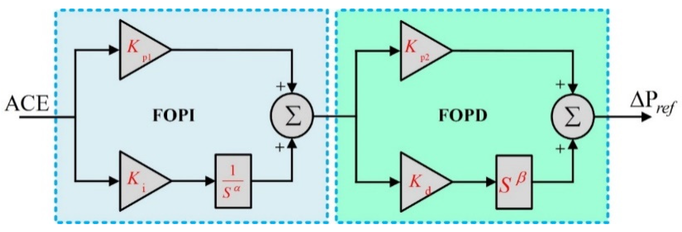
Figure 4.
The structure of multi-stage FOPID controller.

Figure 5.
Flowchart of non-dominated sorting genetic algorithm (NSGA-II) [56].
Figure 5.
Flowchart of non-dominated sorting genetic algorithm (NSGA-II) [56].
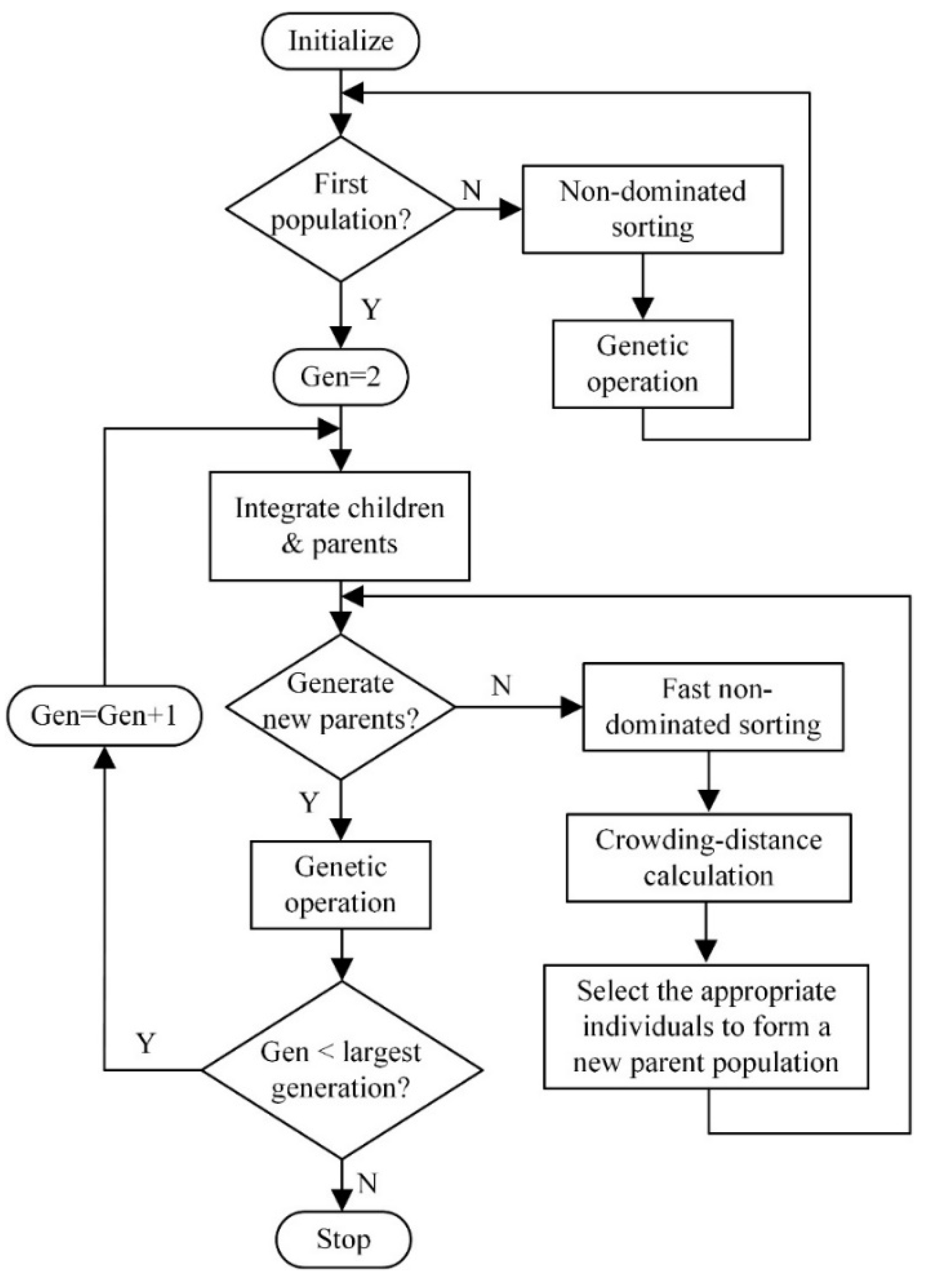
Figure 6.
A Pareto front of the multi-objective problem.
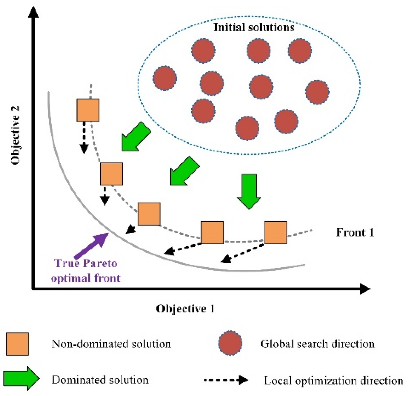
Figure 7.
Process of HiL setup based on OPAL-RT (a) illustration of real-time simulation, (b) compilation process.
Figure 7.
Process of HiL setup based on OPAL-RT (a) illustration of real-time simulation, (b) compilation process.

Figure 8.
POF for FO (PI + PD) cascade controller.
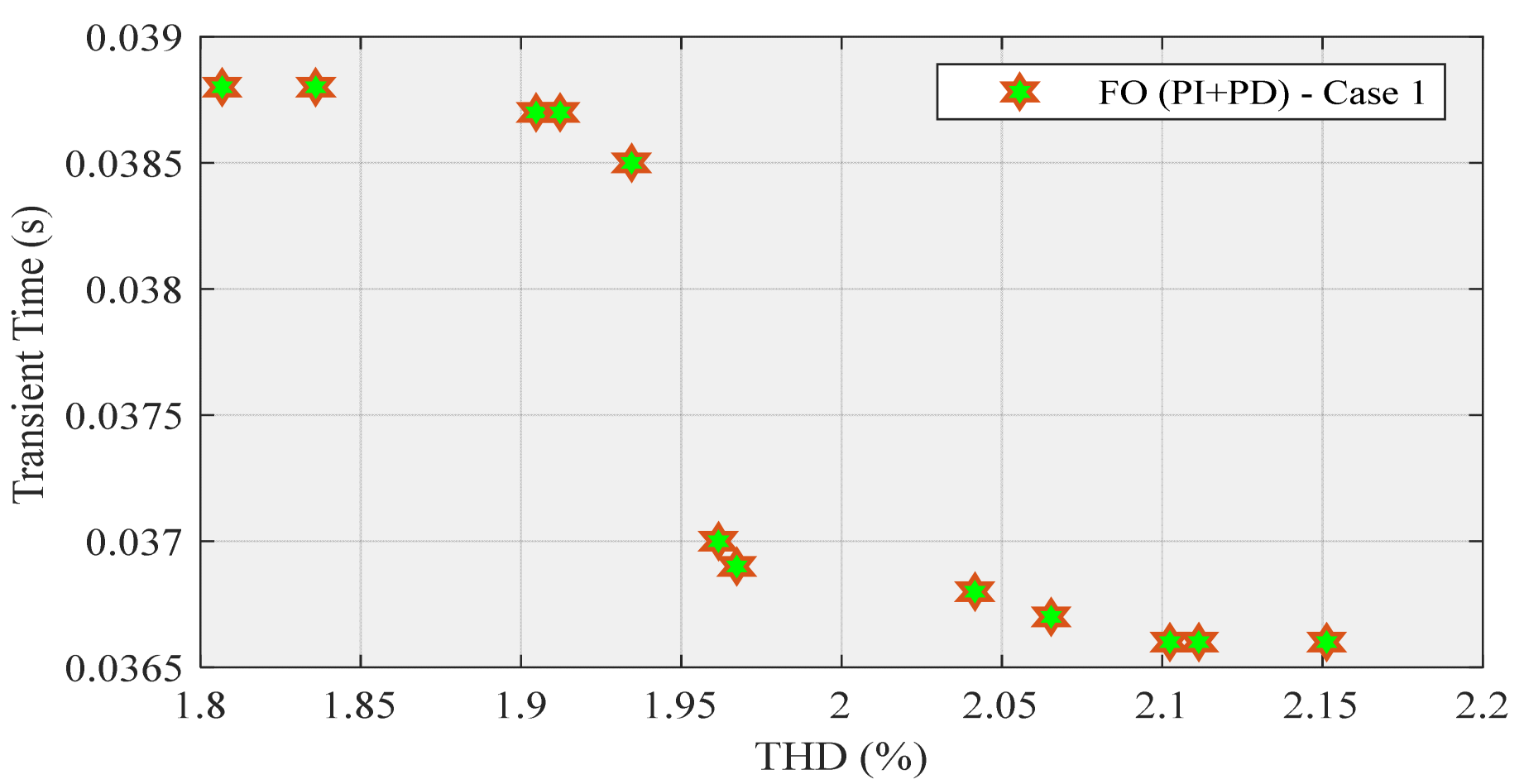
Figure 9.
Compensated source current for row no. 6 (Lowest THD) using FO (PI + PD) cascade controller.
Figure 9.
Compensated source current for row no. 6 (Lowest THD) using FO (PI + PD) cascade controller.

Figure 10.
Row no. 6 (with the lowest THD at steady-state) using FO (PI + PD) cascade controller.

Figure 11.
Compensated source current for row no. 9 (Highest THD) using FO (PI + PD) cascade controller.
Figure 11.
Compensated source current for row no. 9 (Highest THD) using FO (PI + PD) cascade controller.
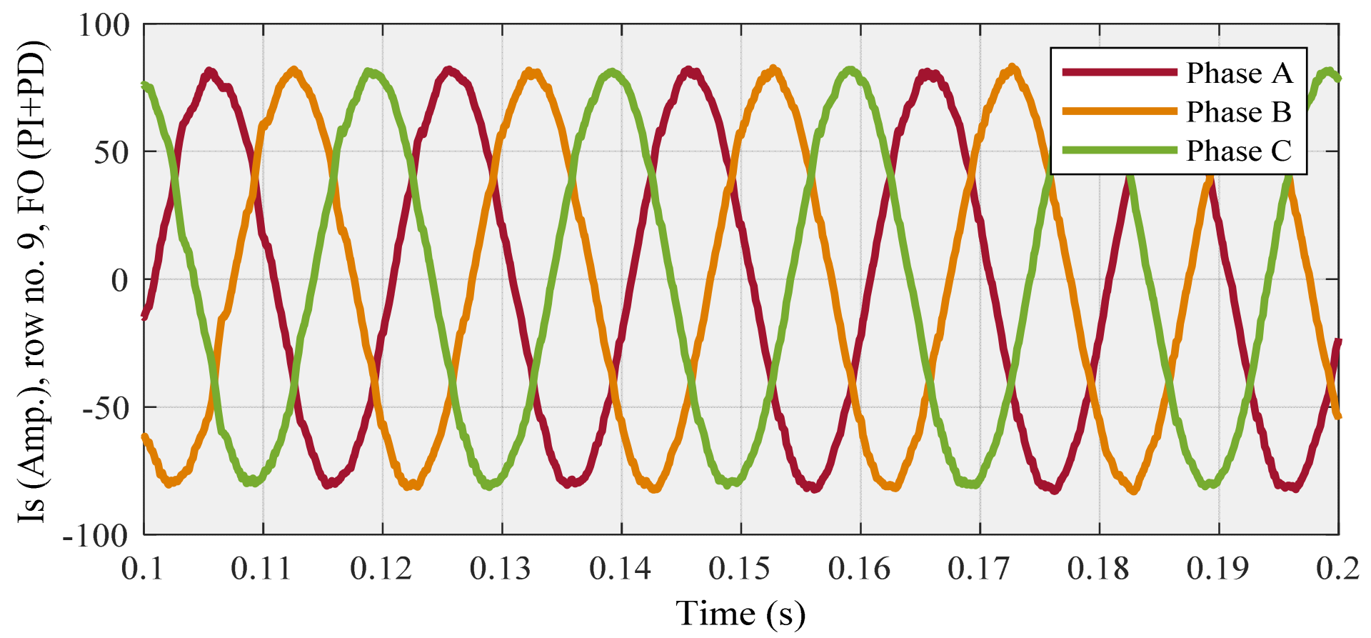
Figure 12.
Row no. 9 (with the highest THD at steady-state) using FO (PI + PD) cascade controller.
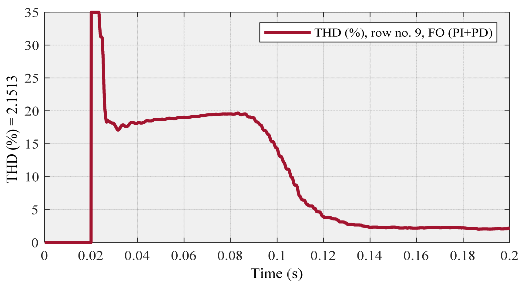
Figure 13.
POF for multistage FOPID.
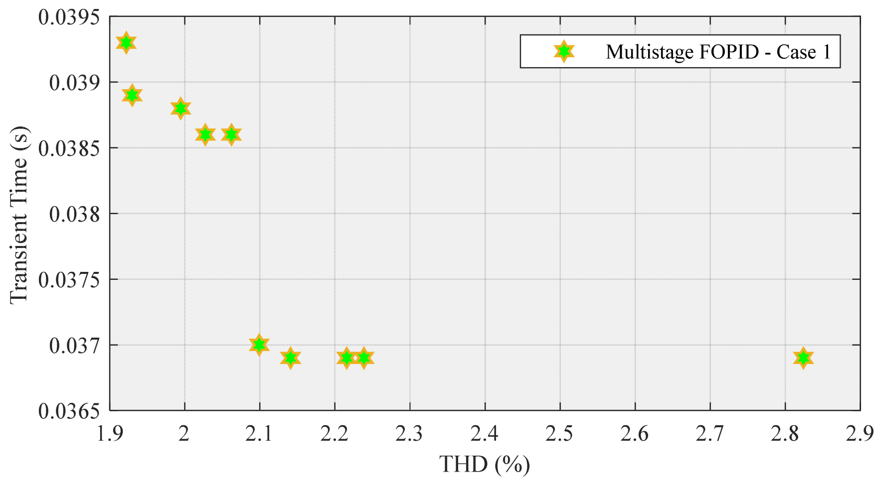
Figure 14.
Compensated source current for row no. 2 (lowest THD) using the multistage FOPID controller.
Figure 14.
Compensated source current for row no. 2 (lowest THD) using the multistage FOPID controller.
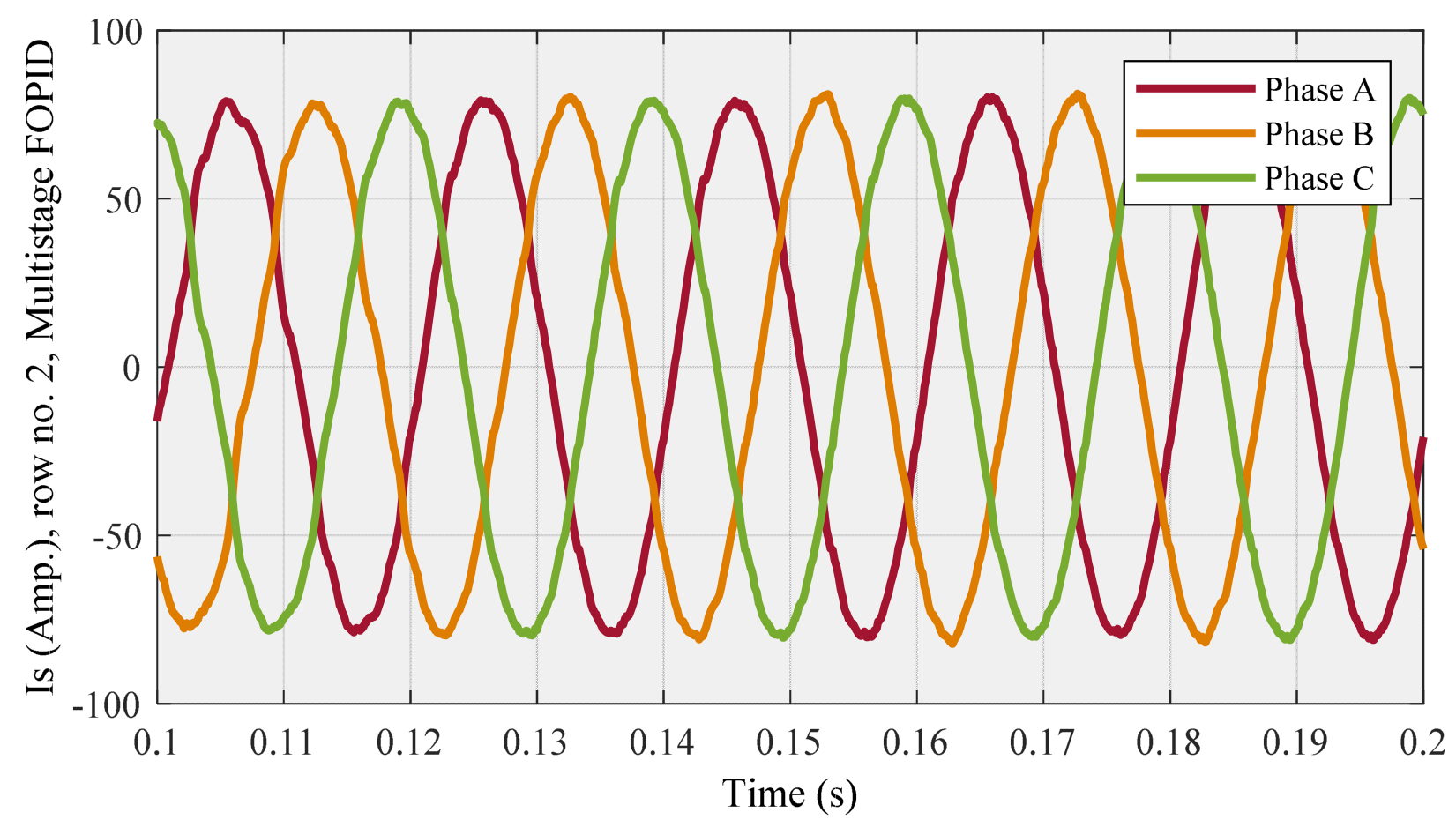
Figure 15.
Row no. 2 (with the lowest THD at steady-state) using a multistage FOPID controller.
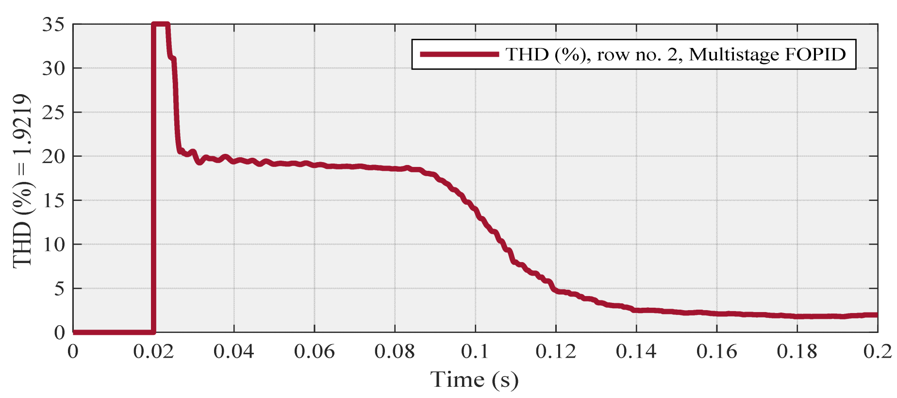
Figure 16.
Compensated source current for row no. 7 (highest THD) using a multistage FOPID controller.
Figure 16.
Compensated source current for row no. 7 (highest THD) using a multistage FOPID controller.
Figure 17.
Row no. 7 (with the highest THD at steady-state) using a multistage FOPID controller.
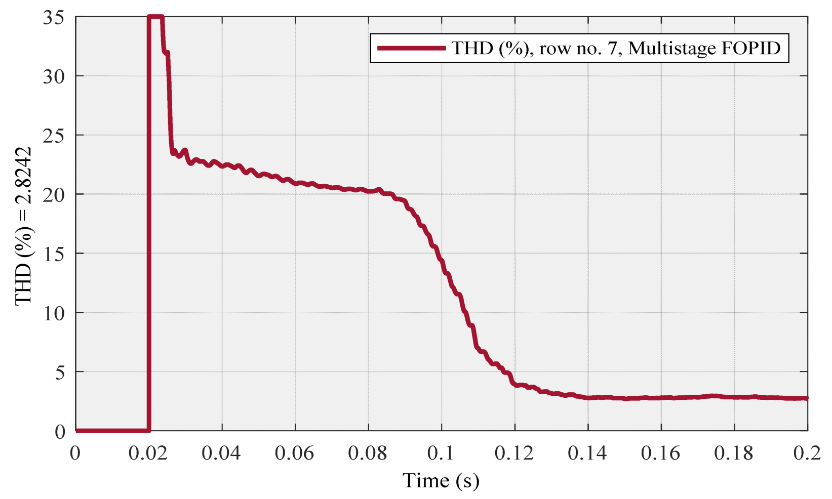
Figure 18.
POF of FO (PI + PD) cascade and multistage FOPID controller—a comparison.
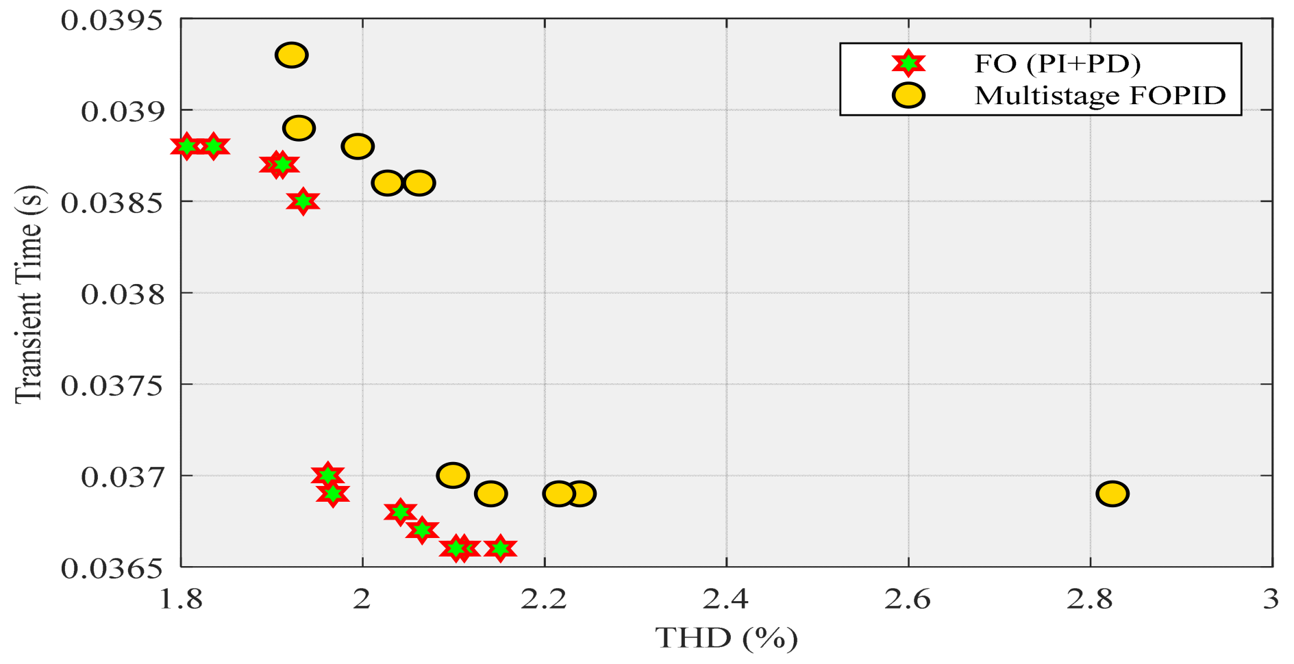


Figure 21.
POF for FO (PI + PD) cascade controller.

Figure 22.
Compensated source current for row no. 1 (THD = 1.8429) using FO (PI + PD) cascade controller.
Figure 22.
Compensated source current for row no. 1 (THD = 1.8429) using FO (PI + PD) cascade controller.
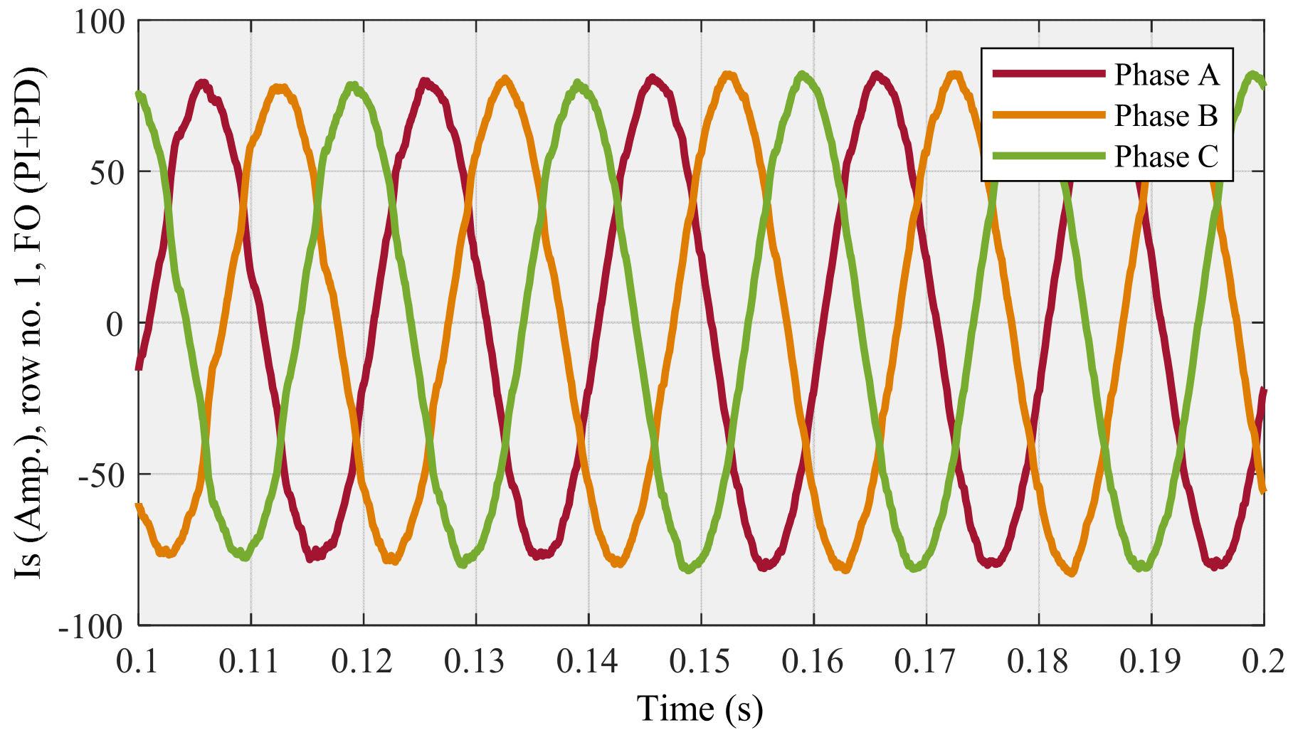
Figure 23.
Row no. 1 (with THD = 1.8429 at steady-state) using FO (PI + PD) cascade controller.
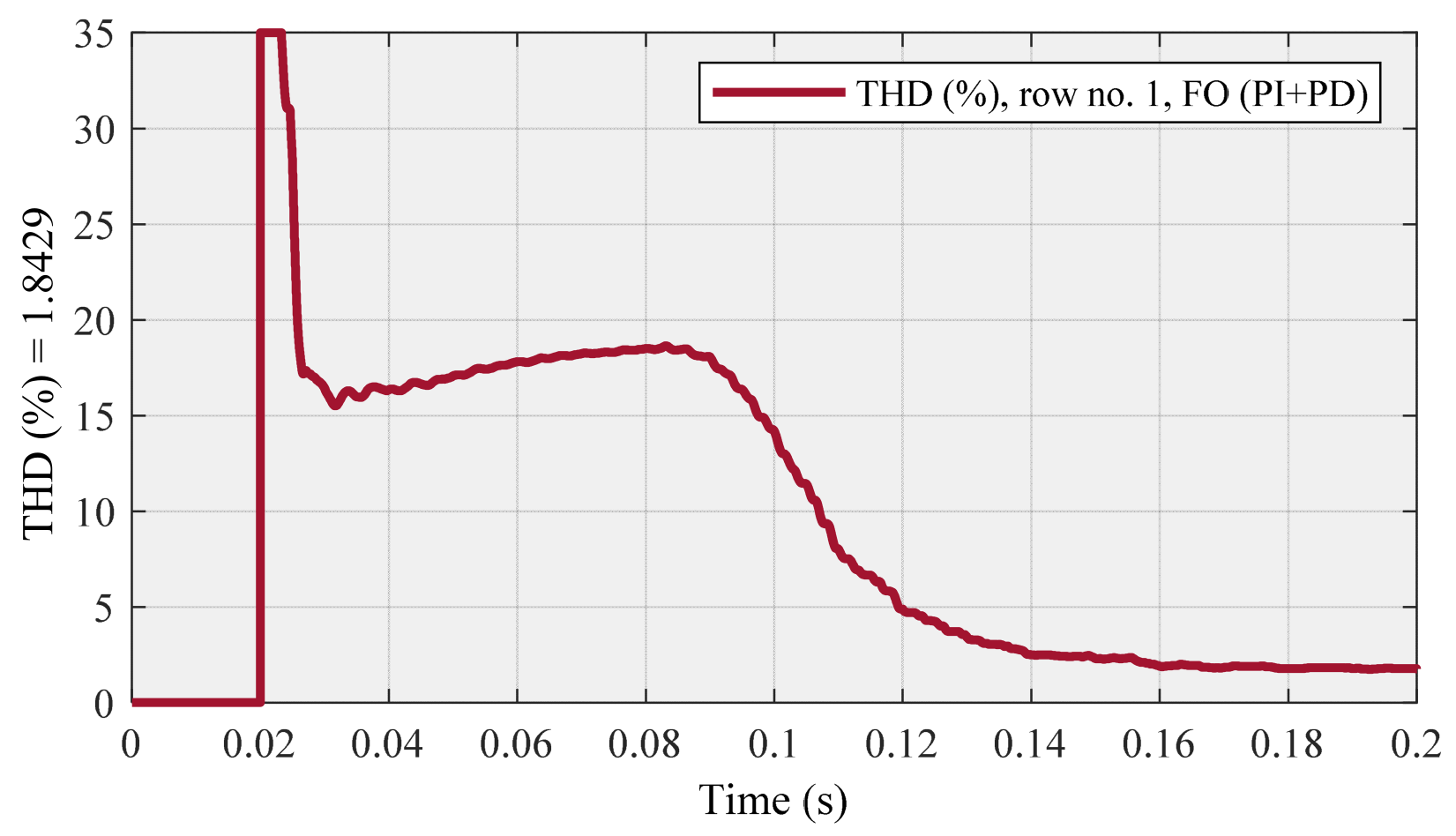
Figure 24.
Compensated source current for row no. 7 (highest THD) using FO (PI + PD) cascade controller.
Figure 24.
Compensated source current for row no. 7 (highest THD) using FO (PI + PD) cascade controller.
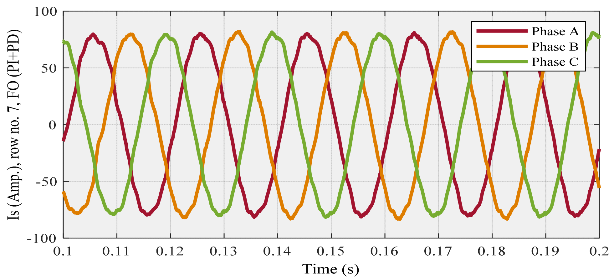
Figure 25.
Row no. 7 (with the highest THD at steady-state) using FO (PI + PD) cascade controller.
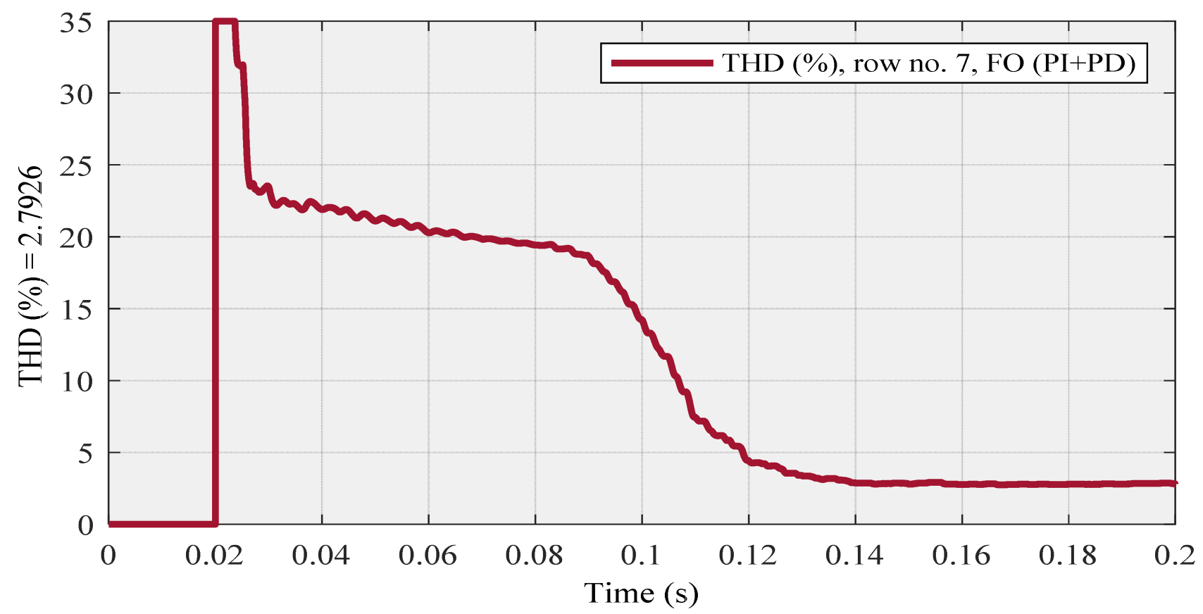
Figure 26.
POF for multistage FOPID controller.
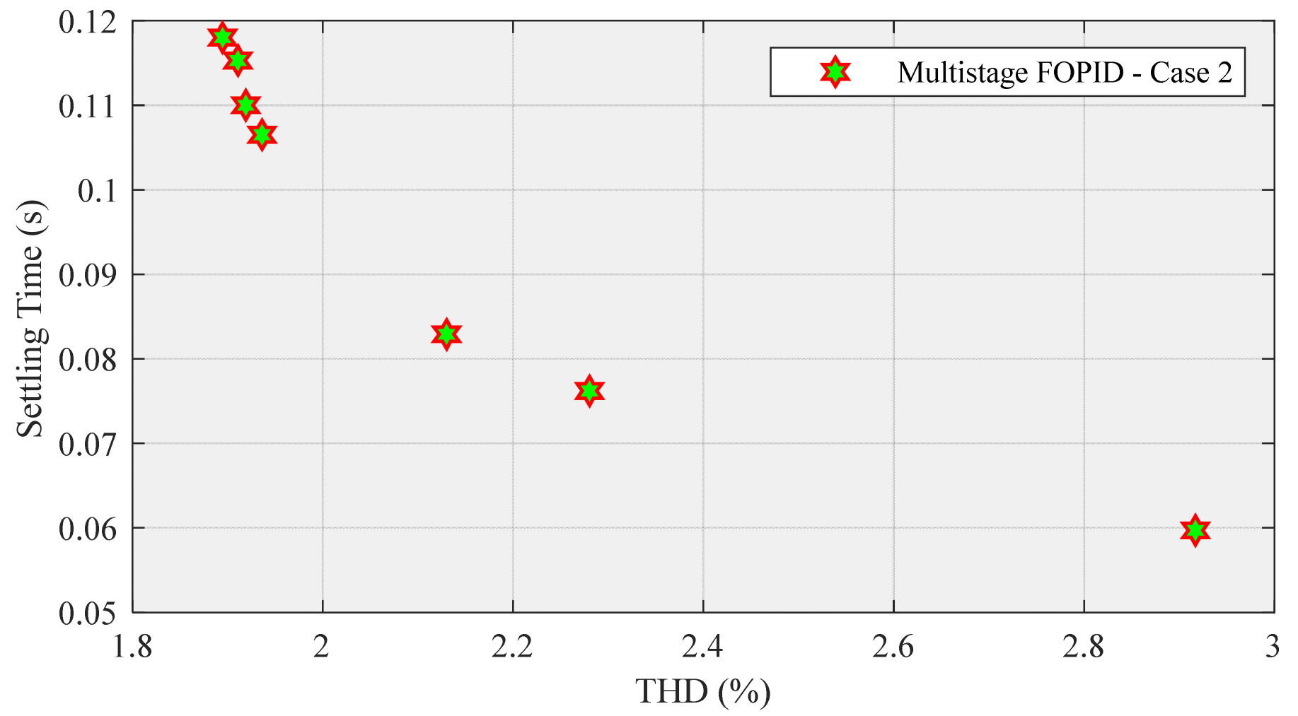
Figure 27.
Compensated source current for row no. 1 (lowest THD) using multistage FOPID controller.
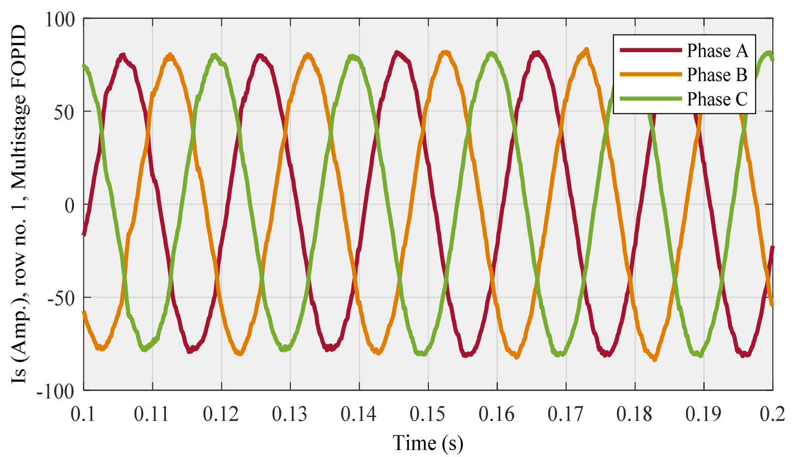
Figure 28.
Row no. 1 (with the lowest THD at steady-state) using multistage FOPID controller.
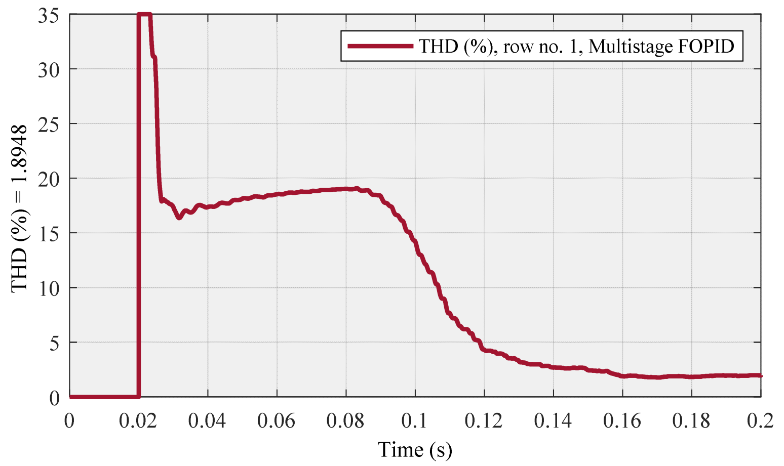
Figure 29.
Compensated source current for row no. 3 (highest THD) using multistage FOPID controller.
Figure 29.
Compensated source current for row no. 3 (highest THD) using multistage FOPID controller.
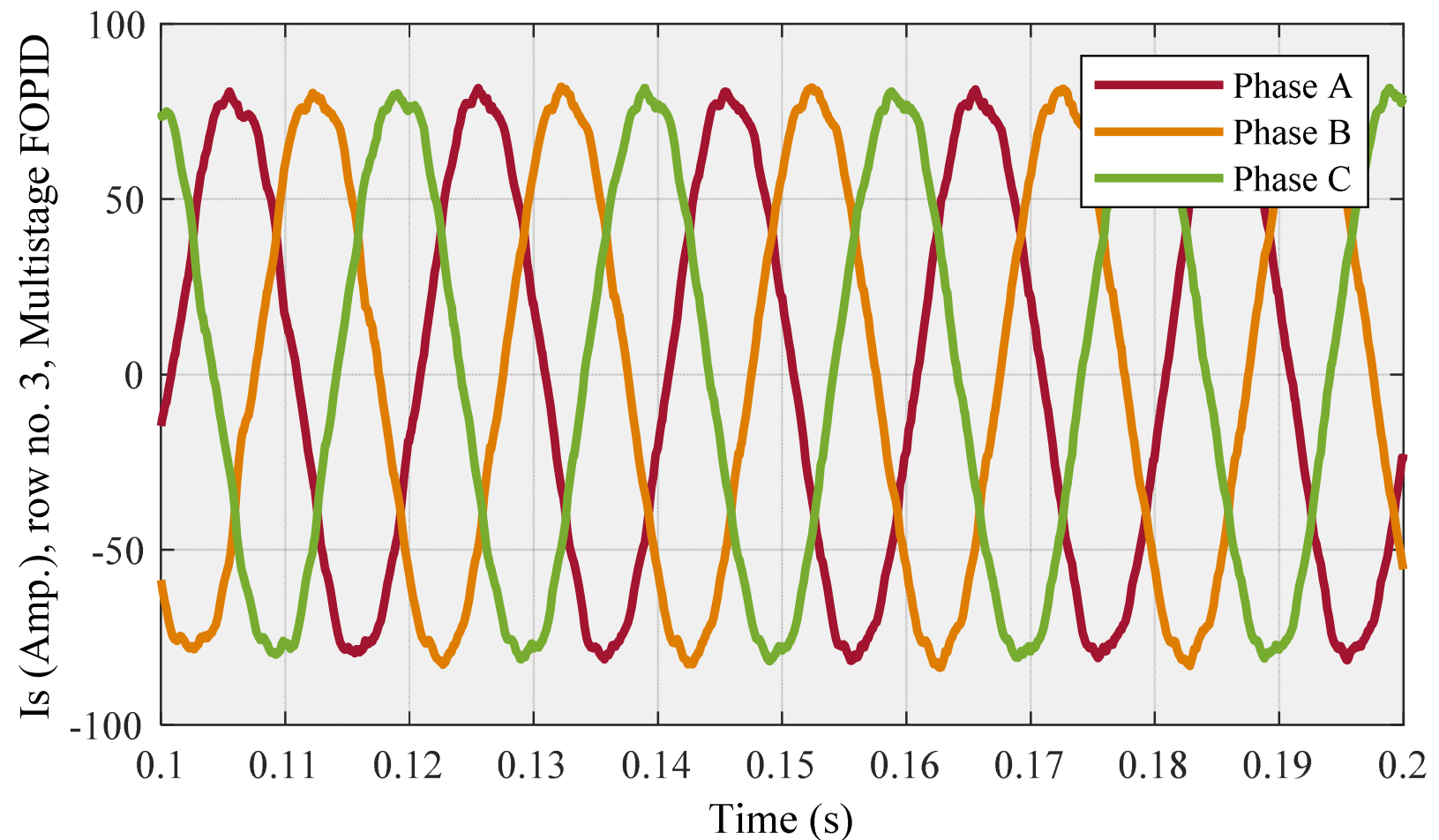
Figure 30.
Row no. 3 (with the highest THD at steady-state) using multistage FOPID controller.

Figure 31.
POF of FO (PI + PD) cascade and multistage FOPID controller—a comparison.


Table 1.
POS and POF for FO (PI + PD) cascade controller.
| No | Kp1 | Ki | Vdc | Kp2 | Kd | α | β | THD (%) | |
|---|---|---|---|---|---|---|---|---|---|
| 1 | 2.4154 | 10.4602 | 815.0000 | 3.0000 | 0.4257 | 0.7481 | 0.3224 | 1.9673 | 0.0369 |
| 2 | 2.0321 | 10.4680 | 815.0000 | 2.5807 | 0.4287 | 0.7496 | 0.3224 | 1.9048 | 0.0387 |
| 3 | 1.9759 | 12.4680 | 815.0000 | 3.0000 | 0.4257 | 0.7481 | 0.3224 | 2.0416 | 0.0368 |
| 4 | 2.2689 | 12.4055 | 815.0000 | 3.0000 | 0.4287 | 0.7481 | 0.3224 | 2.0654 | 0.0367 |
| 5 | 1.9759 | 12.4680 | 815.0000 | 2.5807 | 0.4287 | 0.7481 | 0.3216 | 1.8360 | 0.0388 |
| 6 | 2.0321 | 12.4679 | 814.9904 | 2.5807 | 0.4287 | 0.7481 | 0.3224 | 1.8068 | 0.0388 |
| 7 | 2.2689 | 12.4055 | 814.9904 | 2.5807 | 0.4287 | 0.7481 | 0.3224 | 1.9122 | 0.0387 |
| 8 | 2.4154 | 10.4602 | 815.0000 | 2.9902 | 0.4703 | 0.7481 | 0.3302 | 2.1114 | 0.0366 |
| 9 | 2.2970 | 12.4680 | 814.6924 | 3.0000 | 0.4257 | 0.7481 | 0.3224 | 2.1513 | 0.0366 |
| 10 | 2.4154 | 10.4602 | 814.9994 | 2.9902 | 0.4257 | 0.7481 | 0.3224 | 2.1024 | 0.0366 |
| 11 | 2.4154 | 10.4602 | 815.0000 | 2.9207 | 0.4287 | 0.7481 | 0.3224 | 1.9616 | 0.0370 |
| 12 | 2.4154 | 10.4602 | 815.0000 | 2.5807 | 0.4287 | 0.7480 | 0.3212 | 1.9345 | 0.0385 |
Table 2.
POS and POF for multistage FOPID controller.
| No | Kp | Ki | Vdc | Kpp | N | Kd | α | β | THD (%) | |
|---|---|---|---|---|---|---|---|---|---|---|
| 1 | 2.5400 | 12.4261 | 719.0607 | 11.2424 | 1.7693 | 0.9098 | 0.9000 | 0.0287 | 2.0274 | 0.0386 |
| 2 | 1.8393 | 10.7355 | 573.2281 | 11.7506 | 1.6734 | 0.1000 | 0.9408 | 0.0904 | 1.9219 | 0.0393 |
| 3 | 2.6000 | 13.2472 | 601.7378 | 11.7506 | 1.6734 | 0.6063 | 0.9041 | 0.0287 | 2.0992 | 0.0370 |
| 4 | 2.6000 | 10.0000 | 812.8484 | 11.7428 | 1.0054 | 0.2728 | 0.9683 | 0.0760 | 2.0621 | 0.0386 |
| 5 | 2.5315 | 13.8570 | 812.8484 | 11.7424 | 1.7693 | 0.2728 | 0.9683 | 0.0535 | 1.9946 | 0.0388 |
| 6 | 2.4969 | 13.8570 | 812.8484 | 11.6879 | 1.7547 | 0.9098 | 0.9683 | 0.0287 | 1.9299 | 0.0389 |
| 7 | 2.5764 | 11.1837 | 529.0360 | 11.3453 | 1.6186 | 0.4805 | 0.9335 | 0.0801 | 2.8242 | 0.0369 |
| 8 | 2.5764 | 11.5726 | 686.4316 | 11.9324 | 1.5213 | 0.6709 | 0.9335 | 0.0960 | 2.2386 | 0.0369 |
| 9 | 2.5764 | 11.5745 | 686.4515 | 11.9324 | 1.5213 | 0.6709 | 0.9336 | 0.0967 | 2.1409 | 0.0369 |
| 10 | 2.5764 | 11.5764 | 686.4515 | 11.9324 | 1.5213 | 0.6709 | 0.9336 | 0.0967 | 2.2158 | 0.0369 |
Table 3.
POS and POF for FO (PI + PD) cascade controller.
| NO | Kp1 | Ki | Vdc | Kp2 | Kd | α | β | THD (%) | |
|---|---|---|---|---|---|---|---|---|---|
| 1 | 1.2000 | 13.9922 | 816.6667 | 2.1886 | 1.2999 | 0.8416 | 0.3667 | 1.8429 | 0.1130 |
| 2 | 1.2000 | 13.9922 | 816.6667 | 2.1618 | 0.0100 | 0.7333 | 0.6349 | 1.8836 | 0.1013 |
| 3 | 2.4667 | 13.4800 | 816.6667 | 2.2449 | 1.2999 | 0.8416 | 0.3667 | 1.7717 | 0.1197 |
| 4 | 3.0667 | 14.2904 | 552.2070 | 3.0000 | 1.3000 | 0.6000 | 0.3667 | 2.7445 | 0.0643 |
| 5 | 2.6000 | 10.0000 | 616.6667 | 2.1667 | 0.8700 | 0.6000 | 0.1000 | 2.0936 | 0.0720 |
| 6 | 2.6000 | 10.0000 | 616.6667 | 2.1618 | 0.8700 | 0.9999 | 0.1000 | 2.0609 | 0.0763 |
| 7 | 2.6000 | 10.0000 | 500.0000 | 2.1618 | 1.3000 | 0.6002 | 0.1000 | 2.7926 | 0.0590 |
Table 4.
POS and POF for multistage FOPID controller.
| NO | Kp | Ki | Vdc | Kpp | N | Kd | α | β | THD (%) | |
|---|---|---|---|---|---|---|---|---|---|---|
| 1 | 2.5434 | 11.0508 | 794.7464 | 11.6264 | 1.3662 | 0.8016 | 0.9822 | 0.0984 | 1.8948 | 0.1180 |
| 2 | 2.5432 | 11.8920 | 763.7147 | 11.9952 | 1.2958 | 0.8016 | 0.9399 | 0.0321 | 2.1301 | 0.0829 |
| 3 | 2.4183 | 11.7547 | 490.0000 | 11.9461 | 0.1583 | 1.0000 | 0.9169 | 0.0886 | 2.9171 | 0.0597 |
| 4 | 2.1557 | 11.8764 | 763.7147 | 11.2523 | 0.2918 | 0.4703 | 0.9822 | 0.0984 | 1.9191 | 0.1100 |
| 5 | 2.1426 | 11.8998 | 763.7147 | 11.2523 | 0.2754 | 0.4703 | 0.9688 | 0.0984 | 1.9363 | 0.1065 |
| 6 | 2.1426 | 11.8920 | 763.7147 | 11.2523 | 0.2918 | 0.8016 | 0.9688 | 0.0666 | 1.9108 | 0.1153 |
| 7 | 2.3213 | 10.6331 | 547.4531 | 11.0189 | 1.2924 | 0.2266 | 0.9267 | 0.0921 | 2.2803 | 0.0762 |
Table 5.
POF for FO (PI + PD) cascade/ Multistage FOPID controller—a comparison.
| NO | Controller | THD (%) | THD (%) | ||
|---|---|---|---|---|---|
| 1 | FO (PI + PD) cascade | 1.8068 | 0.0388 | 1.8429 | 0.1130 |
| 2 | Multistage FOPID | 1.9219 | 0.0393 | 1.8948 | 0.1180 |
| 3 | FO (PI + PD) cascade | 2.1513 | 0.0366 | 2.7926 | 0.0590 |
| 4 | Multistage FOPID | 2.8242 | 0.0369 | 2.9171 | 0.0597 |
Publisher’s Note: MDPI stays neutral with regard to jurisdictional claims in published maps and institutional affiliations. |
© 2022 by the authors. Licensee MDPI, Basel, Switzerland. This article is an open access article distributed under the terms and conditions of the Creative Commons Attribution (CC BY) license (https://creativecommons.org/licenses/by/4.0/).
Share and Cite
MDPI and ACS Style
Nikkhah Kashani, H.; Rouhi Ardeshiri, R.; Gheisarnejad, M.; Khooban, M.-H. Optimal Cascade Non-Integer Controller for Shunt Active Power Filter: Real-Time Implementation. Designs 2022, 6, 32. https://doi.org/10.3390/designs6020032
AMA Style
Nikkhah Kashani H, Rouhi Ardeshiri R, Gheisarnejad M, Khooban M-H. Optimal Cascade Non-Integer Controller for Shunt Active Power Filter: Real-Time Implementation. Designs. 2022; 6(2):32. https://doi.org/10.3390/designs6020032
Chicago/Turabian StyleNikkhah Kashani, Hoda, Reza Rouhi Ardeshiri, Meysam Gheisarnejad, and Mohammad-Hassan Khooban. 2022. "Optimal Cascade Non-Integer Controller for Shunt Active Power Filter: Real-Time Implementation" Designs 6, no. 2: 32. https://doi.org/10.3390/designs6020032