An Evaluation of the Design Parameters of a Variable Bearing Profile Considering Journal Perturbation in Rotor–Bearing Systems

Abstract

A variety of bearing profile designs can be used to improve the performance of a rotor–bearing system in severe conditions, such as operating with a shaft misalignment. Misalignments usually occur due to a deformation of the journal, bearing wear, and installation errors. This paper investigates the effects of bearing design parameters under a 3D journal misalignment for a wide range of length-to-diameter ratios to consider short, finite-length, and long journal bearings. Furthermore, the dynamic response of the system to journal perturbation considering linear and parabolic bearing profiles is also investigated. A numerical solution is identified based on the finite difference method, and the equations of motion are derived based on a linear stability analysis in which the fourth-order Runge–Kutta method is used to obtain the journal trajectories. The results show that both profiles help to enhance the rotor–bearing system’s performance regarding the lubricant layer thickness and pressure distribution, in addition to the shaft critical speed over the entire considered range of length-to-diameter ratios. This enhancement reduces the misalignment negative effects on the system performance. The response of the rotor-bearing system to journal perturbation in the case of the parabolic profile are very close to the perfect alignment case in comparison with a linear modification.

1. Introduction

A journal bearing, as an essential transmission component in industrial applications, typically operates at a wide range of rotational speeds and under heavy load conditions. This type of bearing is used widely in rotating machineries, such as turbines, ship stern shafts, wind power, and many other applications. Furthermore, their tribological characteristics have a direct effect on the safety and reliability of the rotor system [1]. However, the operation of this type of bearing suffers from the presence of misalignments, which occur when the shaft’s axis deviates from its parallelism with the axis of the corresponding bearing. Misalignments are well known to be generated for many reasons, such as thermal expansion, installation errors, external loads, and manufacturing errors [2]. As a result, journal misalignment will, in the end, lead to edge wear due to rough contact [3]. This operation condition negatively affects the general lubrication performance of a rotor–bearing system [4]. Working under severe levels of misalignment reduces the life of a bearing and, subsequently, results in the failure of the mechanical system [2,3,4,5]. Therefore, the minimization of the negative effects of misalignment at the edges of a bearing is an essential subject.

The subject of journal bearing misalignments has drawn significant attention from researchers for decades. Ebrat et al. presented a detailed analysis of the evaluation of the dynamic characteristics of a journal bearing with consideration of bearing deformations [6]. The consequences of shaft deformations on the characteristics of journal bearings were studied by Sun and Gui [7], who found that journal misalignment has negative effects on oil pressure and film thickness distributions. They also found that the moment required to achieve a stable operation increases significantly at large eccentricity ratios and high levels of misalignment. The effect of misalignment on the tribological performance of a journal bearing with a textured surface was investigated by Manser et al. [8]. Their results showed that an increase in the degree of misalignment resulted in increases in the frictional force and maximum pressure. The influences of misalignment on the performance of a journal bearing under a variety of operating conditions and bearing surface features were also investigated by researchers [2,9,10], who found a direct relationship between the drawbacks of the characteristics of the bearings and the level of misalignment. Jamali and Al-Hamood [11] used a 3D model to investigate the effects of misalignments in journal bearings. Their study showed that a 3D misalignment results in a sharp drop in the thickness of the lubricant and a corresponding significant increase in pressure levels. An interested study presented by Song et al. [1] found that the frictional force increases clearly as a result of a shaft deviation in the area of the mixed lubrication regime. A more general model for the journal bearing problem was developed by Padelis G. et al. [12] in order to find relationships among several parameters, such as the misalignment level, the coefficient of friction, and the resulting wear depth. They solved this problem numerically using a wide range of the Sommerfeld number.

Modifications to the bearing profile can be used to reduce the effect of misalignment. One of the attempts to improve the bearing profile was suggested by Nacy [13], who experimentally assessed the effect of edge chamfering on a bearing’s side leakage. Another attempt was made by Bouyer and Fillon [14], who examined defects in the profile of a bearing under misalignment torque. Strzelecki [15] modified awhole bearing’s profile using a hyperboloidal curve. It was found that such a change in the bearing’s profile is useful when the journal bearing is working under misalignment and carrying extreme loads. The stability of a journal bearing with variable geometry was studied by Chasalevris and Dohnal [16]. More recently, the axial profile parameters of a bearing were investigated by Ren et al. [17], who found that using a quadratic profile enhanced the general the journal bearing performance. An extensive review of simulations of the journal bearing lubrication problem was presented by Allmaier and Offner [18]. Several topics were addressed in their study, such as polymer coatings, the lubrication regime, and the effect of using low-viscosity lubricants. Their review emphasized that the safe operation of journal bearings is still encountering new challenges, which therefore require more developments in solution methods for overcoming the previously mentioned problems. Atlassi et al. [19] investigated the combined effects of surface roughness and a ferrofluid lubricant on the load-carrying capacity and many other aspects of finite-length journal bearings.

Previous works did not investigate the effects of different forms of bearing profile modifications on the characteristics of misaligned journal bearings. Therefore, this paper addresses these effects by considering a wide range of bearing length-to-diameter ratios, which means studying the effects of the geometrical design parameters on short, finite-length, and long journal bearings. The bearing profile was modified at the edges using linear and curved modifications, and comprehensive comparisons between the results of the two types of profiles are presented. A 3D general misalignment model was used in this work to accurately simulate misalignments in the vertical and horizontal planes, using a numerical solution where the finite difference discretization was considered. Furthermore, the rotor dynamic behavior under journal position perturbation was also considered in the analyses on the base of linear stability analyses where the 4th-order Runge–Kutta method was used to determine the time response of the rotor–bearing system.

2. Equations Related to the Hydrodynamic Lubrication Regime

Figure 1 shows a perfectly aligned journal bearing where the shaft axis is parallel to the bearing axis. In such an ideal case, the resulting gap (lubricant layer thickness) between the shaft surface and the bush inner surface is given by Equation (1), and the general solution is governed by the well-known Reynolds equation (Equation (2)) [11,20].

$$h=c(1+{\epsilon }_r \cos \left(\theta -\varnothing \right))$$

(1)

$$\frac{\partial }{\partial x}\left(\frac{\rho h^3}{12\eta }\frac{\partial p}{\partial x}\right)+\frac{\partial }{\partial z}\left(\frac{\rho h^3}{12\eta }\frac{\partial p}{\partial z}\right)=U_m \frac{\partial \rho h}{\partial x}+\frac{\partial \rho h}{\partial t}$$

(2)

where $h$ represents film thickness, $c$ is radial clearance, ${\epsilon }_r$ $\left(e/c\right)$ is the eccentricity ratio, $e$ is the distance between the shaft and bearing centers, $\varnothing$ represents the attitude angel, $\theta$ is the position angle, $p$ represents the pressure, $\rho$ is density of the lubricant, $\eta$ is lubricant viscosity, $U_m$ is mean velocity, and $t$ is time.

Figure 1. Simplified drawing of an ideal case (without Mis.). (a) Side view and (b) Three-dimensional representation.

In this work, the solution of Equation (2) (this equation is a partial differential equation) is based on the use of the Reynolds boundary conditions method, which requires the satisfaction of the following conditions [21]:

▪

The pressure value: $p=0$ at position $\theta =0$

▪

The pressure gradient and the pressure value: $\frac{\partial p}{\partial \theta }=p=0$ at position $\theta ={\theta }_c$.

where ${\theta }_c$ is the position of the cavitation zone, which can be determined via an iterative solution [21,22].

The current model is written in a dimensionless form using the following relations:

$$H=\frac{h}{c}=R\theta , P=\frac{p-p_o}{6\eta \omega }\left(\frac{c^2}{R^2}\right), \mathrm{and} Z=\frac{z}{L}$$

Using these variables, Equations (1) and (2) are given as follows,

$$H=1+{\epsilon }_r \cos \left(\theta -\varnothing \right)$$

(3)

$$\frac{\partial }{\partial \theta }\left(H^3\frac{\partial P}{\partial \theta }\right)+\alpha \frac{\partial }{\partial Z}\left(H^3\frac{\partial P}{\partial Z}\right)-\frac{\partial H}{\partial \theta }=0$$

(4)

where:

$$\alpha =\frac{1}{4{\left(\mathrm{L}/\mathrm{D}\right)}^2}=\frac{R^2}{L^2}$$

The supported load in a dimensionless form ($\overline{W}=\frac{w}{6\eta \omega RL}{\left(\frac{c}{R}\right)}^2)$ is given as follows,

$$\overline{W}=\sqrt{{\overline{W_r}}^2+{\overline{W_t}}^2}$$

(5)

where

$$\overline{W_r}={{\displaystyle \int }}_0^1{{\displaystyle \int }}_0^{{\theta }_{cav}}P \cos \theta d\theta dz$$

(6)

$$\overline{W_t}={{\displaystyle \int }}_0^1{{\displaystyle \int }}_0^{{\theta }_{cav}}P \sin \theta d\theta dz$$

(7)

The equation of the attitude angle is [23]:

$$\varnothing ={\tan }^{-1}\left(\frac{W_t}{W_r}\right)$$

(8)

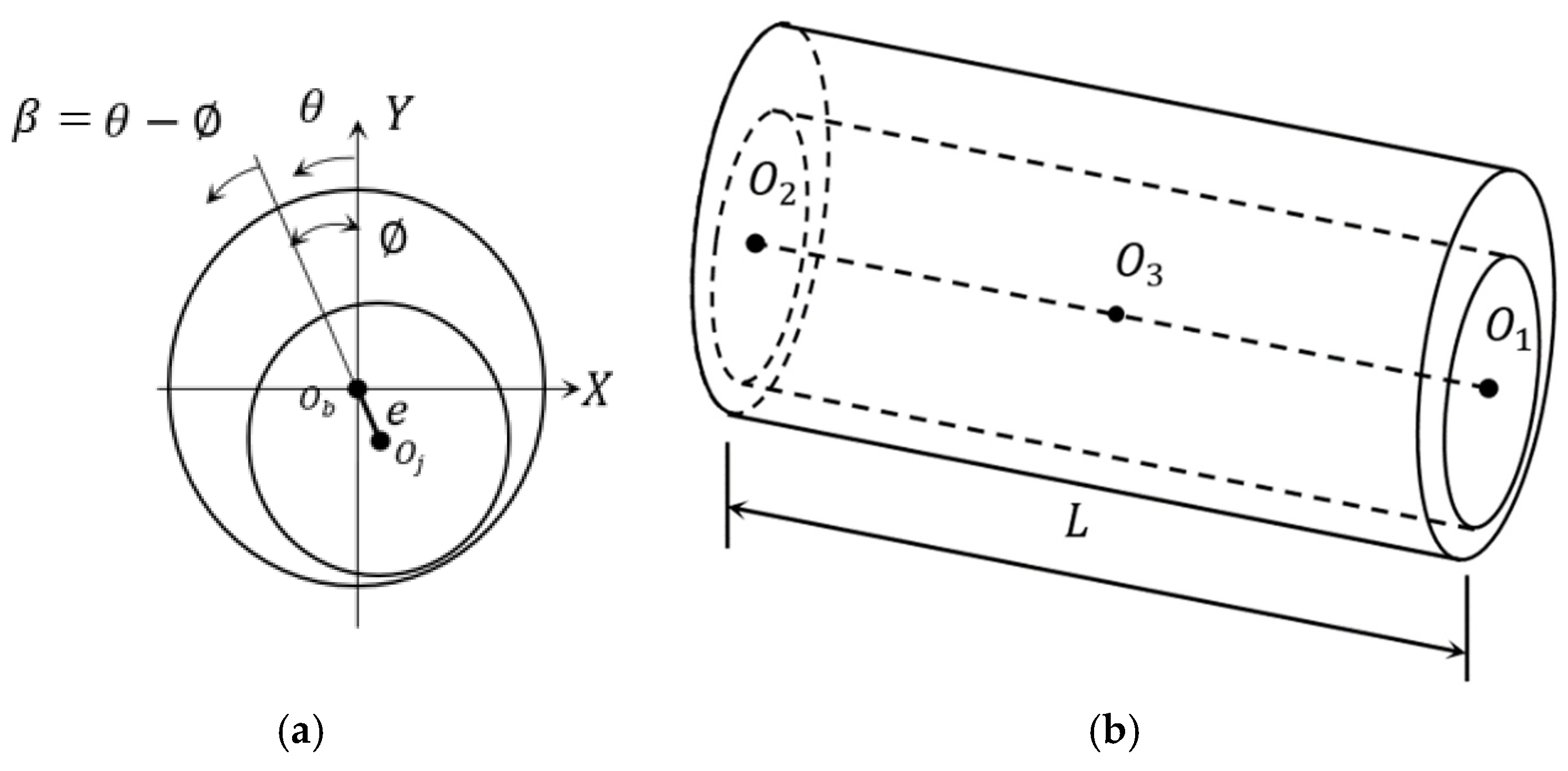
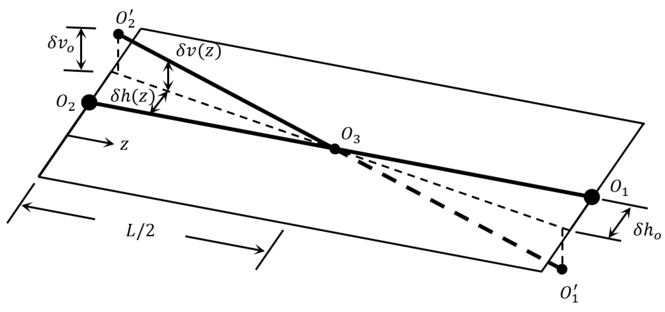
3. Three-Dimensional Misalignment Model

The three-dimensional model of misalignment that shown in Figure 2 identifies the deviations in the vertical and horizontal planes, representing a comprehensive misalignment description. This model is essentially adopted from a previous work [11]. The following equations are used in this model:

$$\begin{gathered} \Delta v\left(Z\right)=\Delta v_o \left(1-2Z\right) for Z\le 1/2 \\ \Delta v\left(Z\right)=\Delta v_o \left(2Z-1\right) for Z>1/2 \\ \Delta h\left(Z\right)=\Delta h_o \left(1-2Z\right) for Z\le 1/2 \\ \Delta h\left(Z\right)=\Delta h_o \left(2Z-1\right) for Z>1/2 \end{gathered}$$

(9)

Figure 2. Model of the 3D misalignment.

These equations are also written in a dimensionless form for the purpose of consistency with the other equations used in the current work, where $\mathsf{\Delta }=\delta /c$ and $\mathrm{Z}=z/L$, as explained previously. This modeling of the misalignment provides a more realistic illustration for both the horizontal $\left(\Delta h\left(z\right)\right)$ as well as the vertical ($\Delta v\left(z\right))$ journal deviations, which are given in terms of the position: $Z$ along the bearing width and the maximum vertical ($\Delta v_o)$ and horizontal $\left(\Delta h_o\right)$ deviations at the bearing edges.

As a result of shaft deviation, attitude angle and the eccentricity are no longer constant along the $z$ direction as in the ideal case, and they vary according to the $Z$ position, as follows [11],

$$\varnothing \left(z\right)={\tan }^{-1}\frac{e_m\sin {\varnothing }_m+\delta h\left(z\right)}{e_m\cos {\varnothing }_m-\delta v\left(z\right)} \mathrm{when} z\le L/2$$

$$e\left(z\right)=\sqrt{{\left(e_m\cos {\varnothing }_m-\delta v\left(z\right)\right)}^2+{\left(e_m\sin {\varnothing }_m+\delta h\left(z\right)\right)}^2}$$

(10)

$$\varnothing \left(z\right)={\tan }^{-1}\frac{e_m\sin {\varnothing }_m-\delta h\left(z\right)}{e_m\cos {\varnothing }_m+\delta v\left(z\right)} \mathrm{when} z>L/2$$

$$e\left(z\right)=\sqrt{{\left(e_m \cos {\varnothing }_m+\delta v\left(z\right)\right)}^2+{\left(e_m \sin {\varnothing }_m-\delta h\left(z\right)\right)}^2}$$

where

${\varnothing }_m$ is the attitude angle at $z=L/2.$

$e_m$ is the eccentricity at $z=L/2.$

These equations and Equation (1) can be used to determine the gap resulting from the misalignment at any position in the z direction.

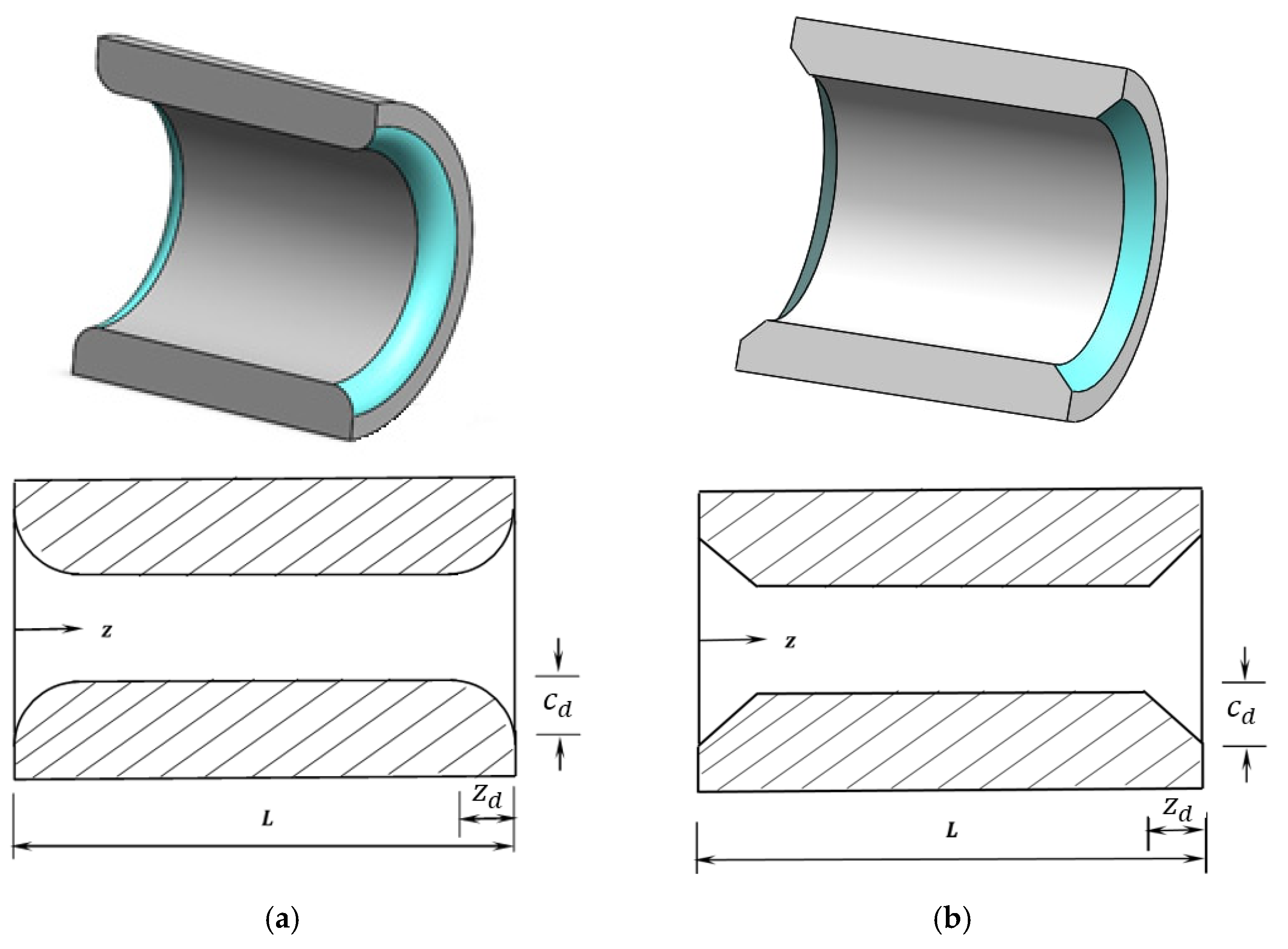
4. Design of the Bearing Profile

The presence of misalignment causes a severe reduction in the layer thickness of the lubricant at the edges of the bearing, as explained previously. This is due to the resulting slope of the shaft in comparison with the axis of the bearing. The thinning of the gap between the surface of the shaft and the inner surface of the bearing can be overcome to an acceptable level by modifying the design of the bearing profile over the positions where the misalignment causes the most drop in the levels of the lubricant layer thickness. This work considers two types of profile modification, which are the curved modification and the linear modification. In the former type, the bearing profile’s slope continues at the modification’s start position, which requires at least a second-order curve, while this is not the case in the latter type (linear). These two design forms are shown in Figure 3. Figure 3a shows the curved type, and Figure 3b illustrates the linear type of modification. In both forms, the modification is performed over a distance $z_d$ along the bearing width from both sides and over a distance $c_d$ in the radial direction.

Figure 3. Variable bearing profile. (a) Curved Mod and (b) Linear Mod.

Using a dimensionless form for the profile modification, where ${\rm Y}=z_d/L$ and $\Gamma =c_d/c$, the resulting gap due to this modification is a function of the $Z$ position, which can be given as follows,

▪

Curved type:

$$H_d\left(Z\right)=\Gamma \left(\frac{1}{{{\rm Y}}^2} Z^2-\frac{2}{{\rm Y}}Z+1\right) \mathrm{for} Z\le {\rm Y}$$

$$H_d\left(Z\right)=\frac{\Gamma }{{{\rm Y}}^2} \left(Z^2-2\left(1-{\rm Y}\right)Z+{\left(1-{\rm Y}\right)}^2\right) \mathrm{for} Z\ge 1-{\rm Y}$$

(11)

$$H_d\left(Z\right)=0 \mathrm{for} {\rm Y}<Z<1-{\rm Y}$$

▪

Linear type:

$$H_d\left(Z\right)=\Gamma \left(1-Z\frac{1}{{\rm Y}}\right) \mathrm{for} Z\le {\rm Y}$$

$$H_d\left(Z\right)=\Gamma \left(1+\frac{1}{{\rm Y}}\left(Z-1\right)\right) \mathrm{for} Z\ge 1-{\rm Y}$$

(12)

$$H_d\left(Z\right)=0 \mathrm{for} {\rm Y}<Z<1-{\rm Y}$$

Using the dimensionless forms of the profile parameters with regard to bearing width (${\rm Y}=z_d/L$) and radial clearance ($\Gamma =c_d/c)$ also better visualizes the total material removal to compensate for the reduced gap due to the 3D misalignment.

In the numerical discretization of the journal bearing problem with the consideration of the 3D misalignment in addition to the bearing profile change, the film thickness is identified by the coupling of the related Equations (3) and (9)–(12).

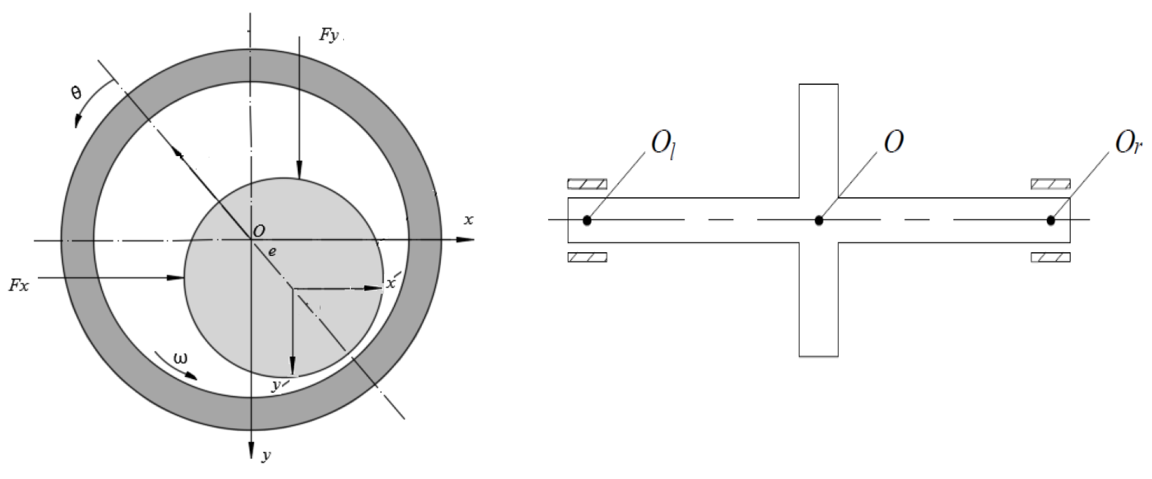
5. Dynamic Characteristics of the Rotor–Bearing System

The determination of the dynamic characteristics of the rotor–bearing system is carried out in this work based on the theory of linear stability analysis, which essentially linearizes the nonlinear forces close to the steady state location ((equilibrium state) of the shaft center.

This analysis considers the time-dependent part in the Reynolds equation (Equation (13)) to derive the stiffness and damping coefficients, which will be used later to determine the critical speed of the rotor in addition to identifying the dynamic response to position perturbation.

$$\frac{\partial }{\partial x}\left(\frac{h^3}{12\eta }\frac{\partial p}{\partial x}\right)+\frac{\partial }{\partial z}\left(\frac{h^3}{12\eta }\frac{\partial p}{\partial z}\right)=\frac{U_j}{2} \frac{\partial h}{\partial x}+\frac{\partial h}{\partial t}$$

(13)

Equation of the film thickness is given in [24]

$$h=h_0+\Delta x\cos \theta +\Delta y\sin \theta$$

(14)

The time-dependent term in Reynold equation ($\frac{\partial h}{\partial t}$) is written as

$$\frac{\partial h}{\partial t}=\Delta \dot{x}\cos \theta +\Delta \dot{y}\sin \theta$$

(15)

The use of the dimensionless variables for Equations (13) and (15) gives

$$\frac{\partial }{\partial \theta }\left(H^3\frac{\partial P}{\partial \theta }\right)+\alpha \frac{\partial }{\partial Z}\left(H^3\frac{\partial P}{\partial Z}\right)=\frac{\partial H}{\partial \theta }+2(\Delta \dot{Y}\sin \theta +\Delta \dot{X }\cos \theta )$$

(16)

where

$$\dot{X}=\frac{R\dot{x}}{Uc} , \dot{Y}=\frac{R\dot{y}}{Uc}$$

(17)

The hydrodynamic forces in terms of the velocity and displacement in both directions are [23,25],

$$\begin{gathered} F_x=F_x (x, y, \dot{x}, \dot{y}) \\ {F}_y=F_y (x, y, \dot{x}, \dot{y}) \end{gathered}$$

$$F_x={{\displaystyle \int }}_0^1{{\displaystyle \int }}_0^{{\theta }_c}P\cos \theta d\theta dZ$$

$$F_y=\underset{0}{\overset{1}{{\displaystyle \int }}}\underset{0}{\overset{{\theta }_c}{{\displaystyle \int }}}P\sin \theta d\theta dZ$$

(18)

From which the total force is $F=\sqrt{F_x{}^2+F_y{}^2}$.

Therefore, the determination of the eight dynamic coefficients is performed using the following equations [26],

$$\left[k\right]=\left[\begin{array}{cc}{k}_{xx}& k_{xy}\\ k_{yx}& k_{yy}\end{array}\right]=\left[\begin{array}{cc}\frac{\partial F_x}{\partial X}& \frac{\partial F_x}{\partial Y}\\ \frac{\partial F_y}{\partial x}& \frac{\partial F_y}{\partial Y}\end{array}\right]$$

(19)

$$\left[c\right]=\left[\begin{array}{cc}{c}_{xx}& c_{xy}\\ c_{yx}& c_{yy}\end{array}\right]=\left[\begin{array}{cc}\frac{\partial F_x}{\partial \dot{X}}& \frac{\partial F_x}{\partial \dot{Y}}\\ \frac{\partial F_y}{\partial \dot{X}}& \frac{\partial F_y}{\partial \dot{Y}}\end{array}\right]$$

(20)

The suggested form for the dynamic coefficients by [25] is used in the current work as follows

$$K_{xx}=\frac{c k_{xx}}{F}, K_{xy}=\frac{c k_{xy}}{F}, K_{yx}=\frac{c k_{yx}}{F}, K_{yy}=\frac{c k_{yy}}{F}$$

(21)

$$C_{xx}=\frac{c \omega c_{xx}}{F}, C_{xy}=\frac{c \omega c_{xy}}{F}, C_{yx}=\frac{c \omega c_{yx}}{F} , C_{yy}=\frac{c \omega c_{yy}}{F}$$

(22)

The use of Equations (3), (19) and (20) gives

$$\begin{gathered} K_{xx}={{\displaystyle \int }}_0^1{{\displaystyle \int }}_0^{2\pi }{P}_x \cos \theta d\theta dz \\ {K}_{xy}={{\displaystyle \int }}_0^1{{\displaystyle \int }}_0^{2\pi }{P}_y \cos \theta d\theta dz \\ {K}_{yx}={{\displaystyle \int }}_0^1{{\displaystyle \int }}_0^{2\pi }{P}_x \sin \theta d\theta dz \end{gathered}$$

$$\begin{gathered} K_{yy}={{\displaystyle \int }}_0^1{{\displaystyle \int }}_0^{2\pi }{P}_y \sin \theta d\theta dz \\ {C}_{xx}={{\displaystyle \int }}_0^1{{\displaystyle \int }}_0^{2\pi }{P}_{\dot{x}} \cos \theta d\theta dz \end{gathered}$$

$$C_{xy}={{\displaystyle \int }}_0^1{{\displaystyle \int }}_0^{2\pi }{P}_{\dot{y}} \cos \theta d\theta dz$$

$$C_{yx}={{\displaystyle \int }}_0^1{{\displaystyle \int }}_0^{2\pi }{P}_{\dot{x}} \sin \theta d\theta dz$$

$$C_{yy}={{\displaystyle \int }}_0^1{{\displaystyle \int }}_0^{2\pi }{P}_{\dot{y}} \sin \theta d\theta dz$$

where

$$P_x=\frac{\partial P}{\partial X}, P_y=\frac{\partial P}{\partial Y}, P_{\dot{x}}=\frac{\partial P}{\partial \dot{X}}, P_{\dot{y}}=\frac{\partial P}{\partial \dot{Y}}$$

The identification of the eight dynamic coefficients involves calculating the following derivative,

$$\begin{gathered} \hspace{1em}\hspace{1em}\hspace{1em}\hspace{1em}\hspace{1em}\frac{\partial H}{\partial t}=\Delta \dot{X}\cos \theta +\Delta \dot{Y}\sin \theta \\ \frac{\partial H}{\partial X}=\cos \theta \\ \frac{\partial H}{\partial Y}=\sin \theta \\ \hspace{1em}\hspace{1em}\hspace{1em}\hspace{1em}\hspace{1em}\hspace{1em}\frac{\partial H}{\partial \theta }=-\Delta X \sin \theta +\Delta Y\cos \theta \end{gathered}$$

Furthermore, the differentiation of the governing equation in relation to $\dot{X},$ $\dot{Y, }$ $X$ and $Y$ gives

$$\frac{\partial }{\partial \theta }\left(H^3\frac{\partial P_x}{\partial \theta }\right)+\alpha \frac{\partial }{\partial Z}\left(H^3\frac{\partial P_x}{\partial Z}\right)=-\frac{\partial }{\partial \theta }\left(3H^2\cos \theta \frac{\partial P}{\partial \theta }\right)-\alpha \frac{\partial }{\partial Z}\left(3H^2\cos \theta \frac{\partial P}{\partial Z}\right)-\sin \theta$$

(23)

$$\frac{\partial }{\partial \theta }\left(H^3\frac{\partial P_y}{\partial \theta }\right)+\alpha \frac{\partial }{\partial Z}\left(H^3\frac{\partial P_y}{\partial Z}\right)=-\frac{\partial }{\partial \theta }\left(3H^2\sin \theta \frac{\partial P}{\partial \theta }\right)-\alpha \frac{\partial }{\partial Z}\left(3H^2\sin \theta \frac{\partial P}{\partial Z}\right)-\cos \theta$$

(24)

$$\frac{\partial }{\partial \theta }\left(H^3\frac{\partial P_{\dot{x}}}{\partial \theta }\right)+\alpha \frac{\partial }{\partial Z}\left(H^3\frac{\partial P_{\dot{x}}}{\partial Z}\right)=\cos \theta$$

(25)

$$\frac{\partial }{\partial \theta }\left(H^3\frac{\partial P_{\dot{y}}}{\partial \theta }\right)+\alpha \frac{\partial }{\partial Z}\left(H^3\frac{\partial P_{\dot{y}}}{\partial Z}\right)=\sin \theta$$

(26)

Determining the pressure derivatives involves a numerical discretization of Equations (23)–(26) to calculate the eight dynamic coefficients. The determination of the dynamic response of the journal to position perturbation is performed after calculating the previously mentioned eight dynamic coefficients. Figure 4 illustrates a schematic drawing of a rotor–bearing system where the equations of motion of this system can be written as follows [27].

$$m {\ddot{x}}^{\prime }=-F_x+f_{ex}-f\sin \Omega t$$

(27)

$$m {\ddot{y}}^{\prime }=-F_y+f_{ey}-f\cos \Omega t+W$$

(28)

where [27,28]

Figure 4. The considered system ([28] edited).

$F_x, F_y$: bearing forces

$f$: unbalance force

$f_{ex}$, $f_{ey}$: external loads

$x^{\prime }$, $y^{\prime }$: axes of whirling around the steady state position.

The equations of motion ((27) and (28)) can be written using dimensionless variables as follows

$$\overline{M}{\ddot{X}}^{\prime }=-{\overline{F}}_x+{\overline{F}}_{ex}-\overline{Ru} \sin T$$

(29)

$$\overline{M}{\ddot{Y}}^{\prime }=-{\overline{F}}_y+{\overline{F}}_{ey}-\overline{Ru} \cos T+1$$

(30)

where

$${\overline{F}}_x=\frac{F_x}{W} , {\overline{F}}_y=\frac{F_y}{W} \overline{M}=\frac{m c{ \mathsf{\Omega }}^2}{W} \mathrm{and} \overline{Ru}=m_u r\frac{{\Omega }^2}{W}$$

The system’s dynamic response is obtained by solving Equations (29) and (30) [29]. The critical speed is determined from these equations after neglecting all external and unbalanced forces,

$$\overline{M}{\ddot{X}}^{\prime }+{\overline{F}}_x=0$$

(31)

$$\overline{M}{\ddot{Y}}^{\prime }+{\overline{F}}_y=0$$

(32)

The bearing forces are given in [25]

$$\overline{F}x=K_{xx} X^{\prime }+K_{xy} Y^{\prime }+C_{xx} {\dot{X}}^{\prime }+C_{xy} {\dot{Y}}^{\prime }$$

(33)

$$\overline{F}y=K_{yx} X^{\prime }+K_{yy} Y^{\prime }+C_{yx} {\dot{X}}^{\prime }+C_{yy} {\dot{Y}}^{\prime }$$

(34)

The substitution of these equations in Equations (31) and (32) and using the following solution suggested by [24], $X^{\prime }=A{e}^{i\lambda t}$ and $Y^{\prime }=B{e}^{i\lambda t}$, we can obtain

$$(keq-K_{xx})(keq-K_{yy})-{\lambda }^2{C}_{xx}{C}_{yy}-K_{xy}{K}_{yx}+{\lambda }^2{C}_{xy}{C}_{yx}=0$$

(35)

where

$$\lambda =\sqrt{\frac{\left(keq-K_{xx}\right)\left(Keq-K_{yy}\right)-K_{xy} K_{yx}}{C_{xx} C_{yy}-C_{xy}{C}_{yx}}}$$

(36)

$$Keq=\frac{K_{xx} C_{yy}+K_{yy}{C}_{xx}-K_{yx}{C}_{xy}-K_{xy}{C}_{yx}}{C_{xx}+C_{yy}}$$

(37)

$${\Omega }_{crit}=\frac{\sqrt{keq}}{\lambda }$$

(38)

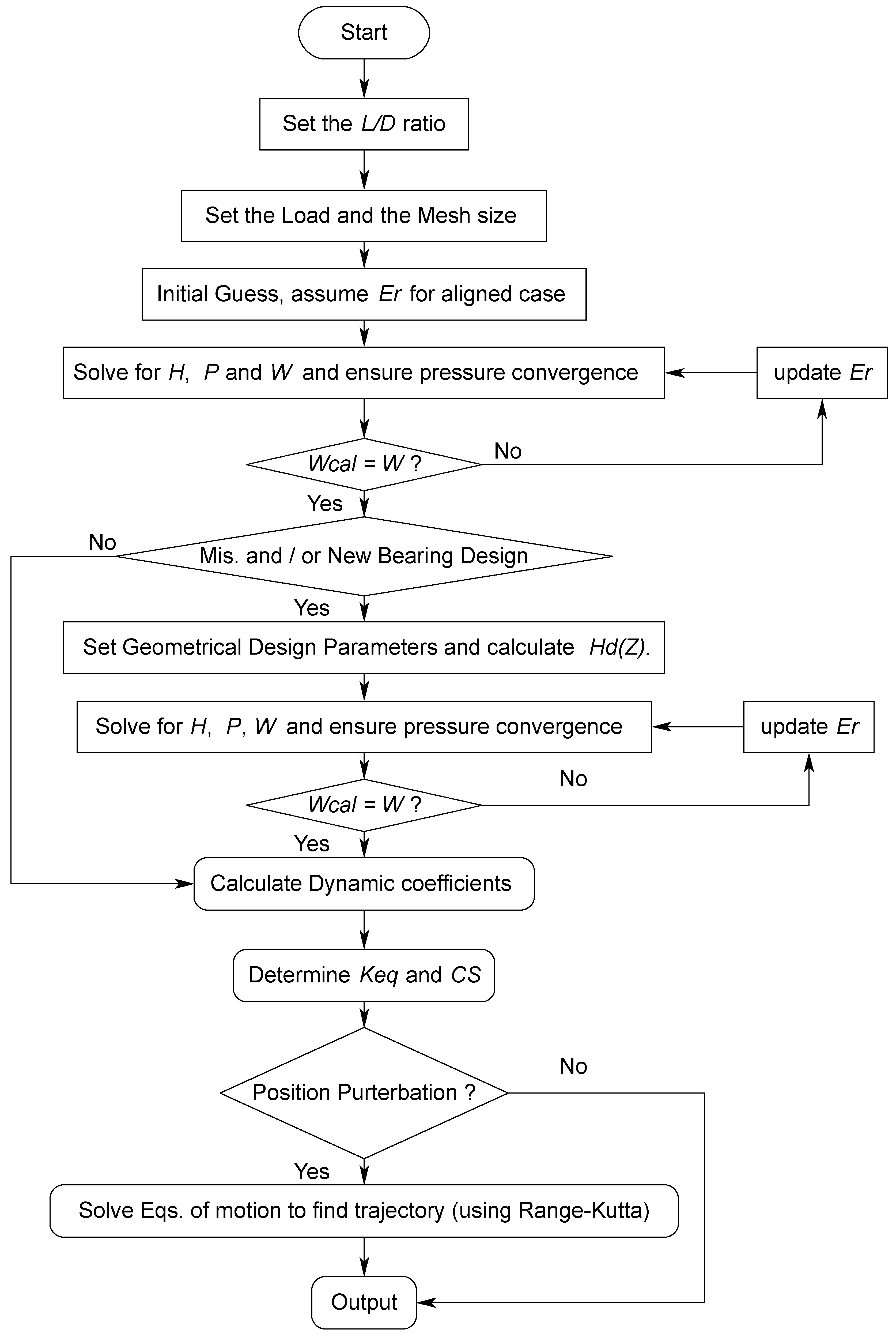
6. Numerical Solution

The numerical solution of a finite-length journal bearing problem under the effect of 3D misalignment and modified bearing profile is performed by discretizing the governing equations which are the Reynolds equation and the resulting equation of the total gap due to misalignment and profile variation. The discretization is performed based on the finite difference method. Then, the resulting equations are solved through the use of the Gauss–Sedial method under a successive over-relaxation solution. The converged solution provides the film thickness and the pressure distribution, which are used to determine the eight dynamic coefficients (stiffness and damping). At this stage, the equations of motion can now be solved using the fourth-order Runge–Kutta method to determine the dynamic response under position perturbation. The following equations results, after discretizing the governing equations, are used to determine the pressure distribution in the iterative solution,

$$P_{\left(i, j\right)}=\frac{1}{\beta }\left[H_b{}^3 P_{\left(i+1, j\right)}+H_a{}^3 P_{\left(i-1, j\right)}+\alpha C_2{H}_c{}^3 P_{\left(i, j+1\right)}+\alpha C_2{H}_d{}^3 P_{\left(i, j-1\right)}-C_1{H}_{\left(i+1, j\right)}+C_1{H}_{\left(i-1, j\right)}\right]$$

(39)

$$H\left(i, j\right)=\left(1+{\epsilon }_r\left(Z\right)\cos ({\theta }_{\left(i, j\right)}-\varnothing \right))$$

(40)

where $C_1=0.5 \Delta \theta$, $C_2={\left(\Delta \theta /\Delta Z\right)}^2$, $\beta =H_b{}^3+H_a{}^3+\alpha C_2{H}_c{}^3+\alpha C_2{H}_d{}^3 \mathrm{and} \Delta \theta$, $\Delta Z$ are steps of discretization.

The numerical solution as well as the discretization of the governing equations were explained in detail in Reference [11]. The pressure derivative required to determine the stiffness and damping coefficients in a discrete form is obtained by discretizing Equations (23)–(26), which is

$${\overline{P}}_{\left(i, j\right)}=\frac{1}{\psi }\left[{\left(\Delta \theta \right)}^2 RHS-H_b{}^3 {\overline{P}}_{\left(i+1, j\right)}-H_a{}^3 {\overline{P}}_{\left(i-1, j\right)}-\alpha C_2{H}_c{}^3 {\overline{P}}_{\left(i, j+1\right)}-\alpha C_2{H}_d{}^3 {\overline{P}}_{\left(i, j-1\right)}+C_1{H}_{\left(i+1, j\right)}-C_1{H}_{\left(i-1, j\right)}\right]$$

(41)

where $\psi =-H_b{}^3-H_a{}^3-\alpha C_2{H}_c{}^3-\alpha C_2{H}_d{}^3$.

The right-hand side (RHS) of Equations (23)–(26) is also determined numerically as follows:

$$\begin{gathered} \hspace{1em}RHS\left(22\right)=\frac{\left(3\cos {\theta }_b{H}_b^2+3\cos {\theta }_a{H}_a^2\right)P_{\left(i, j\right)}}{{\left(\Delta \theta \right)}^2}-\frac{3\cos {\theta }_b{H}_b^2{P}_{\left(i+1, j\right)}}{{\left(\Delta \theta \right)}^2}-\frac{3\cos {\theta }_a{H}_a^2{P}_{\left(i-1, j\right)}}{{\left(\Delta \theta \right)}^2}+ \\ \alpha \frac{\left(3\cos {\theta }_c{H}_c^2+3\cos {\theta }_d{H}_d^2\right)P_{\left(i, j\right)}}{{\left(\Delta Z\right)}^2}-\alpha \frac{3\cos {\theta }_c{H}_c^2{P}_{\left(i, j+1\right)}}{{\left(\Delta Z\right)}^2}-\alpha \frac{3\cos {\theta }_d{H}_d^2{P}_{\left(i, j-1\right)}}{{\left(\Delta Z\right)}^2}-\sin \theta \end{gathered}$$

$$\begin{gathered} \hspace{1em}RHS\left(23\right)=\frac{\left(3\sin {\theta }_b{H}_b^2+3\sin {\theta }_a{H}_a^2\right)P_{\left(i, j\right)}}{{\left(\Delta \theta \right)}^2}-\frac{3\sin {\theta }_b{H}_b^2{P}_{\left(i+1, j\right)}}{{\left(\Delta \theta \right)}^2}-\frac{3\sin {\theta }_a{H}_a^2{P}_{\left(i-1, j\right)}}{{\left(\Delta \theta \right)}^2}+ \\ \alpha \frac{\left(3\sin {\theta }_c{H}_c^2+3\sin {\theta }_d{H}_d^2\right)P_{\left(i, j\right)}}{{\left(\Delta Z\right)}^2}-\alpha \frac{3\sin {\theta }_c{H}_c^2{P}_{\left(i, j+1\right)}}{{\left(\Delta Z\right)}^2}-\alpha \frac{3\sin {\theta }_d{H}_d^2{P}_{\left(i, j-1\right)}}{{\left(\Delta Z\right)}^2}-\cos \theta \end{gathered}$$

$$\begin{gathered} RHS\left(24\right)=\cos {\theta }_{\left(i, j\right)} \\ RHS\left(25\right)=\sin {\theta }_{\left(i, j\right)} \end{gathered}$$

At this step, the solution of the whole equations is performed based on a pressure convergence criterion of $\frac{{\displaystyle \sum }\left|P_{\left(i, j\right)new} - P_{\left(i, j\right)old}\right|}{{\displaystyle \sum }{P}_{\left(i, j\right)old}}<{10}^{-7}$. After determining the pressure field, the supported load is determined using numerical integration, and the resulting load is compared with the applied real load with an accuracy of $\mp {10}^{-5}$. If this calculated load is not within this limit, ${\epsilon }_r$ is manipulated, and the whole process of calculating a new pressure field and film thickness is repeated. After obtaining the pressure and the load convergences, the 4th-order Runge–Kutta method is used to solve the equations of motion to determine the system’s dynamic response. Figure 5 shows a flowchart of the solution steps.

Figure 5. Main solution steps.

7. Results and Discussions

This work presents the results in a dimensionless form for the purpose of generality. They can be easily transformed into a dimensional form using the equations explained in the previous sections. The results are divided into subsections as follows.

7.1. Effect of Mesh Density and Validation of the Current Model

Figure 6 shows the effect of mesh density on the values of the dimensionless critical speed and the dimensionless maximum pressure. It can be seen that when the number of nodes is greater than 16,471, the difference is negligible in the critical speed as well as the maximum pressure values. However, the number of nodes adopted in this work is 65,341 to minimize any error related to the discretization of the governing equations.

Figure 6. Effect of mesh density on the dimensionless critical speed and dimensionless maximum pressure.

The results of the current model for the unmodified bearing are compared with Reference [16], where very good agreement is obtained, as shown in Table 1.

Table 1. The comparison between the results of the current work and the result of Reference [17].

Summerfield No.	KXX		KYY
	Ref. [16]	Current Work	Ref. [16]	Current Work
0.319	3.35	3.34	2.10	1.99
1.220	1.62	1.69	2.30	2.21

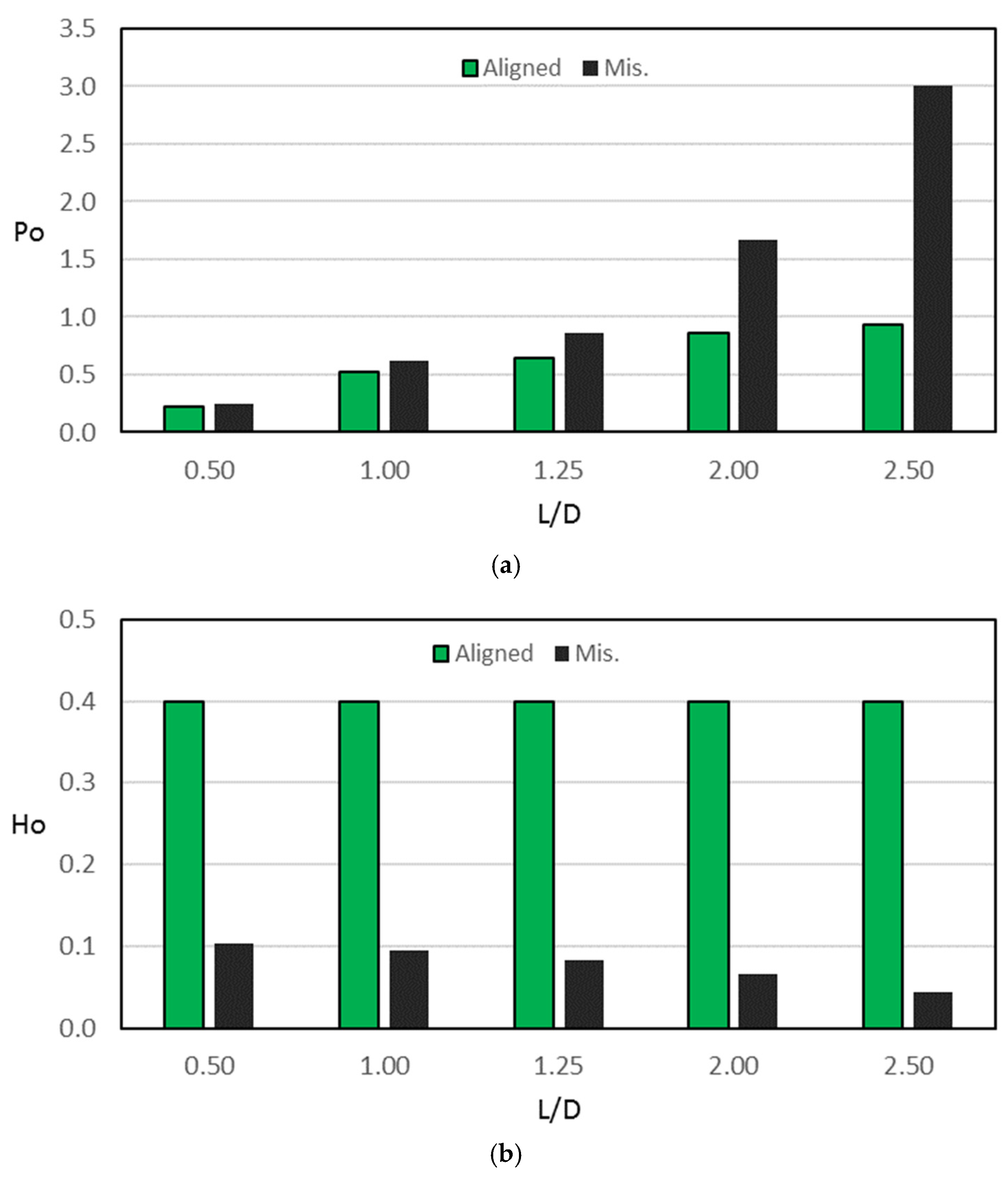
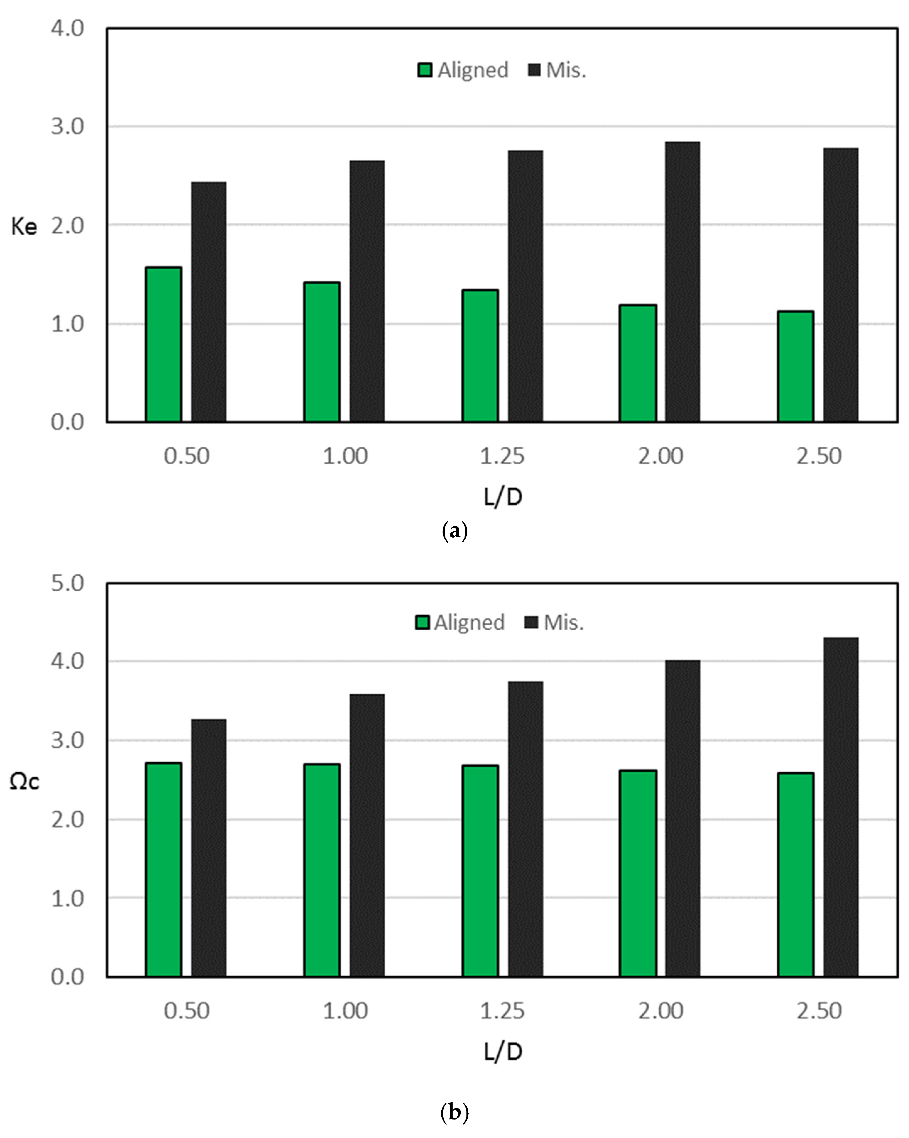
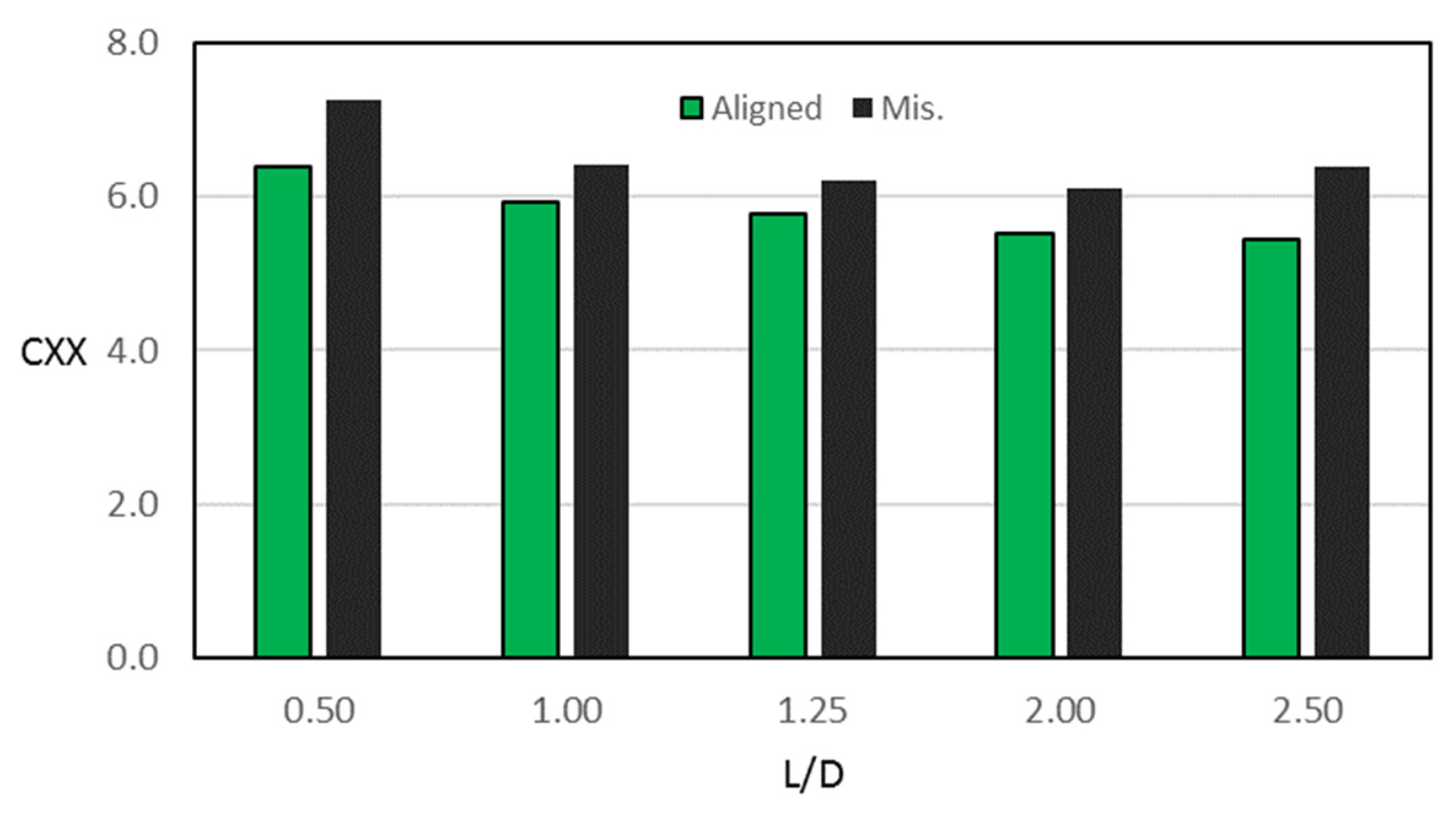
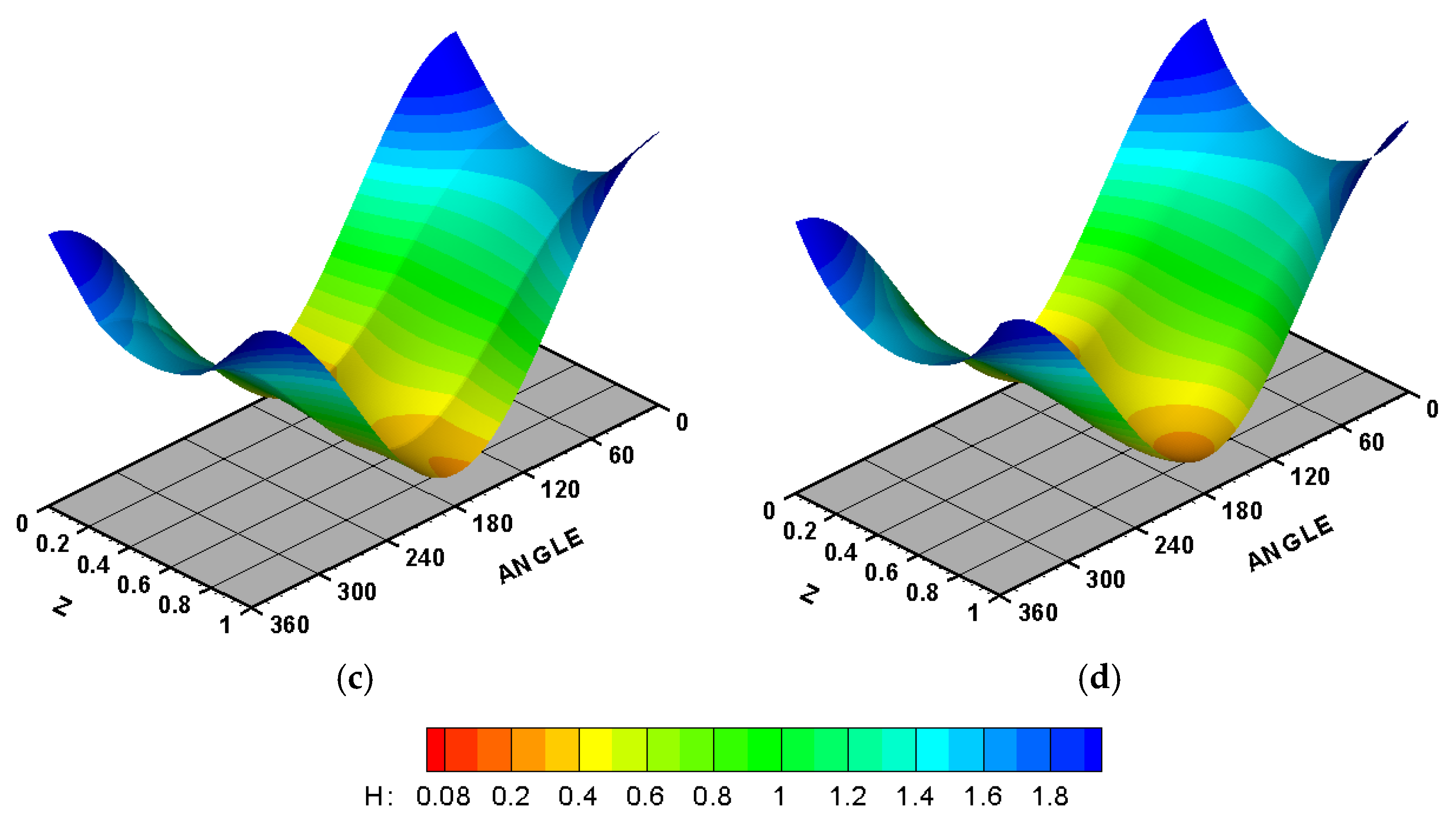
7.2. Effect of the 3D Misalignment on the Characteristics of the System

Figure 7 illustrates the effects of the 3D misalignment for a wide range of Length/Diameter ratios ($L/D$) on the dimensionless maximum pressure ($P_o$) and the dimensionless minimum film thickness ($H_o$) when the eccentricity ratio (${\epsilon }_r)$ is 0.6, and the misalignment parameters are ${\Delta }_v={\Delta }_h=0.56$. It is well known that, in the case of a perfectly aligned journal bearing, increasing the ratio ($L/D)$ for the same ${\epsilon }_r$ increases the resulting maximum pressure, as seen in the green bars shown in Figure 7a. The values of $P_o$ are 0.227, 0.529, 0.644, 0.858, and 0.928 when the ratios $L/D$ are 0.5, 1.0, 1.25, 2.0, and 2.5, respectively. This means, in other words, that changing the $L/D$ ratio from 0.5 to 2.5 for the same eccentricity ratio increases the dimensionless maximum pressure more than three times. The presence of misalignment, which is practically difficult to avoid, increases the maximum pressure values for the whole considered range of $L/D$ ratios, which is illustrated by the black bars in Figure 7a. This increase in the maximum pressure value is more noticeable at the higher $L/D$ ratios. The percentage increases due to the presence of 3D misalignment are 10.5%, 17.1%, 34.2%, 94.1%, and 224.4% for the previously mentioned range of $L/D$ ratios, respectively. Therefore, it is important to avoid higher values of $L/D$ ratios. On the other hand, Figure 7b shows the corresponding misalignment effect on the dimensionless minimum film thickness for the considered range of $L/D$ ratios. In the ideal case of journal bearing, using an eccentricity ratio of 0.6 for the whole range of $L/D$ ratio results in the same dimensionless minimum film thickness values. This is obvious from Equation of the film thickness ($H=1+{\epsilon }_r\cos \theta$), which results in a minimum value of 0.4 when ${\epsilon }_r=0.6$, regardless of the $L/D$ ratio. This value (0.4) can be seen by the green bars in Figure 7b. The 3D misalignment reduces the values of $H_o$ significantly in the whole range of $L/D$ ratio, as illustrated by the black bars in this figure. The reduction is 74.4%, 76.4%, 79.3%, 83.4% and 89.3% when $L/D$ are 0.5, 1.0, 1.25, 2.0, and 2.5, respectively. Such a reduction in the minimum film thickness, which is much less than the designed value, will negatively affect the system’s performance and life. One of the solutions is reducing the supported load value by the journal bearing to elevate the minimum film thickness, but this is not a practical solution. This work will show later how changing the design of the bearing profile will improve the bearing performance with regard to the levels of pressure, film thickness and many other related factors.

Figure 7. Three-dimensional Misalignment effect for a wide range of Length/Diameter ratio on the (a) Dimensionless maximum pressure and (b) dimensionless minimum film thickness; ε_r = 0.6, Δ_v = Δ_h =0.56.

The misalignment also affects the dynamic features of the system. Figure 8 shows the misalignment effects for a wide range of Length/Diameter ratios on the dimensionless equivalent stiffness and the dimensionless critical speed when ${\epsilon }_r=0.6$ and the 3D misalignment parameters are ${\Delta }_v={\Delta }_v=0.56$. It can be seen that (Figure 8a), the equivalent stiffness coefficient ($K_e$) increases by 55.4%, 87.1%, 104.4%, 139.6%, and 147.5% when L/D is 0.5, 1.0, 1.25, 2.0, and 2.5, respectively. These increases in the equivalent stiffness raise the corresponding dimensionless critical speed by 20.5%, 33.0%, 39.7%, 53.3%, and 66.3%, respectively. The improvement in the critical speed of the rotor–bearing system due to the 3D misalignment for the whole range of $L/D$ ratio comes at the price of the reduction in the static characteristics of the considered system, as mentioned previously (Figure 7) in terms of the sharp increase in the maximum pressure and the significant drop in the minimum film thickness. However, changing the bearing profile design parameters will be shown later to be an excellent compromise in terms of maintaining a relatively thick film of lubricant and lowering the maximum pressure without losing a significant part of the enhancement in the dynamic characteristics of the considered system.

Figure 8. Three-dimensional misalignment effect for a wide range of Length/Diameter ratio on the (a) Dimensionless equivalent stiffness coefficient and (b) dimensionless critical speed; ${\epsilon }_r=0.6, {\Delta }_v={\Delta }_h=0.56$.

More details about the consequence of the 3D misalignment on the dynamic coefficients of the considered system are shown in Figure 9 and Figure 10. Figure 9 shows the misalignment effects on the four dimensionless stiffness coefficients ($K_{XX}$, $K_{XY}$, $K_{YX}$ and $K_{YY}$), while Figure 10 illustrates the corresponding effects on the four dimensionless damping coefficients ($C_{XX}$, $C_{XY}=$ $C_{YX}$ and $C_{YY}$). In all cases (the full $L/D$ range), the presence of the 3D misalignment changes all the dynamic coefficients, so the critical speed was changed. It is worth mentioning that the coefficient of stiffness $K_{YX}$ is the first responsible for journal bearing stability. The negative values for this coefficient lead to instability problems, while the positive values result in stable operation of the journal bearing [30].

Figure 9. Effect of 3D misalignment for a wide range of Length/Diameter ratios on the four dimensionless stiffness coefficients; ${\epsilon }_r=0.6, {\Delta }_v={\Delta }_h=0.56$.

Figure 10. Effect of 3D misalignment for a wide range of Length/Diameter ratios on the four dimensionless damping coefficients; ${\epsilon }_r=0.6, {\Delta }_v={\Delta }_h=0.56$.

7.3. Modification Effect on the Characteristics of Misaligned Journal Bearing

The results presented in the previous section showed how the 3D misalignment increased the pressure levels and reduced the film thickness values for the whole considered range of the $L/D$ ratios. These negative consequences of the misalignment can be minimized by changing the bearing design. This section explains the results related to the use of two forms of bearing profiles, which are linear and curved modifications. Figure 11 illustrates the effect of varying the bearing geometry on the dimensionless maximum pressure and the dimensionless minimum film thickness when the design parameters are ${\rm Y}=\Gamma =0.25$. These values of the design parameters are chosen after a series of tests to ensure the use of the optimum values. This figure presents the results of the perfectly aligned, misaligned (3D), and modified bearing. In Figure 11a, both forms of modification reduce the dimensionless maximum pressure, particularly at the higher values of the $L/D$ ratio. For example, when $L/D=2.0$, the dimensionless maximum pressure under misalignment is changed from 1.66 to 1.03 and 1.10 (37.95% and 33.7%) in the case of linear and curved modification, respectively. The curved modification produces slightly higher pressure values at the higher $L/D$ ratios and less value when $L/D<1.25$. On the other hand, changing the profile design has a more obvious and important effect on the dimensionless minimum film thickness, as shown in Figure 11b. It can be seen that the profile modification elevates the thickness of the lubricant significantly for the whole range of $L/D$ ratios. The value of Ho under misalignment when $L/D=1$, for example, changed from 0.094 to 0.271 and 0.258 as a result of the linear and curved modification, respectively. This means, in other words, if the clearance is 50 μm, then the film thickness would change from 4.7 μm in the case of misalignment to 13.55 μm and 12.9 μm due to the linear and curved modification, respectively. These values represent about triple the film thickness value of the corresponding unmodified design under misalignment. It is worth mentioning that Ho is 0.4 for the ideal bearing, which is equivalent to 20 μm for the example of 50 μm clearance. Therefore, improving the minimum film thickness level from 4.7 μm to about 13 μm in both cases represents a significant step in maintaining an acceptable thickness of the lubricant layer.

Figure 11. Consequence of changing the bearing design using two forms of modification on (a) the dimensionless maximum pressure and (b) the dimensionless minimum film thickness: ${\rm Y}=\Gamma =0.25$.

The effects of modification on the 3D pressure distribution and film thickness are better illustrated in Figure 12 and Figure 13. Figure 12 shows the 3D pressure distribution when $L/D=1.0$ (left) and 2.0 (right), and similar behavior is obtained for the other $L/D$ ratios. Therefore, they are not shown here. Figure 12a shows the pressure distribution of the ideal case. In this case, the pressure distribution is uniform (aligned) and symmetric about the line of $z=L/2$. Figure 12b shows the pressure distribution when the system operates under the 3D misalignment, where it is no longer symmetric about the line of $z=L/2$, and pressure spikes appear. These spikes correspond to the positions where the film thickness reduces significantly due to misalignment. Introducing the profile modification reduces these pressure spikes, and the pressure distribution becomes closer to that of the aligned case, particularly at the lower $L/D$ ratio, as shown in Figure 12c, where the curved modification is only shown in this figure as the almost similar shape is obtained for the linear modification. The corresponding film thickness distributions are shown in Figure 13 for the case of $L/D=1.0$, as similar behavior is obtained for the other $L/D$ ratios. Figure 13a shows the film thickness distribution for the perfect case (without misalignment), where the distribution is uniform and extruded in constant values over the length $L$. However, this perfect case seldom exists in the practical uses of journal bearings. The effect of misalignment on the film thickness is shown in Figure 13b, where the distribution is no longer uniform and shows red zones (minimum values) at the bearing edges. The effects of linear and curved modifications on the film thickness distribution are shown in Figure 13c and Figure 13d, respectively. The film thickness is elevated at the edges due to these modifications. The curved modification shows a more uniform distribution as the slope continuity is maintained at the start of modification in contrast with the linear modification, where the sudden change in the profile is obvious in Figure 13c. This sudden change might lead to stress concentration, and an elastohydrodynamic solution is required to assess the linear modification more accurately. However, this is not the case in the curved modification, as explained previously.

Figure 12. Three-dimensional dimensionless pressure distributions when $L/D=1.0$ (left) and $L/D=2.0$ (right). (a) Ideal case, (b) 3D misalignment (${\mathsf{\Delta }}_v={\mathsf{\Delta }}_h=0.56)$ and (c) 3D misalignment (${\mathsf{\Delta }}_v={\mathsf{\Delta }}_h=0.56$) and curved modification $\left({\rm Y}=\Gamma =0.25\right)$.

Figure 13. Three-dimensional dimensionless film thickness when $L/D=1.0$. (a) Ideal case, (b) 3D misalignment (${\mathsf{\Delta }}_v={\mathsf{\Delta }}_h=0.56)$, (c) 3D misalignment (${\mathsf{\Delta }}_v={\mathsf{\Delta }}_h=0.56$) and linear modification $\left({\rm Y}=\Gamma =0.25\right)$ and (d) 3D misalignment (${\mathsf{\Delta }}_v={\mathsf{\Delta }}_h=0.56$) and curved modification $\left({\rm Y}=\Gamma =0.25\right)$.

Figure 14 shows the effect of changing the bearing profile using linear and curved modifications on the dimensionless equivalent stiffness and the dimensionless critical speed of the finite-length journal bearings for the whole considered range of $L/D$ ratios. The increases in the equivalent stiffness (Figure 14a) and in the critical speed (Figure 14b) due to the 3D misalignment are accompanied by the sharp reduction in the thickness of the lubricant layer and the significant increase in the pressure levels, as mentioned previously. Therefore, the assessment of the rotor–bearing performance should consider all the aspects of the system. Using the modified bearing profile has been shown above to have significant positive results in terms of the levels of pressure, levels of film thickness, and the shape of the pressure distribution, which reduces its asymmetricity. Figure 14 illustrates that the modification (both forms) reduces the dimensionless equivalent stiffness and the dimensionless critical speed. However, they are still greater than the corresponding values of the perfectly aligned bearings. This represents an important outcome as both modification forms maintain a higher value of critical speed compared with the perfect aligned case (designed value) in the whole considered range of $L/D$ ratios. As an example, the critical speed (dimensionless value) when $L/D=1$ is 2.694 in the aligned case, which becomes 3.300 and 3.281 using linear and curved modifications, respectively. In other words, this represents an increase of 22.5% and 21.8%, respectively, which represents an additional benefit of the modifications to the major advantage of elevating the value of the minimum film thickness. Similar behavior is also obtained for the other $L/D$ ratios, as illustrated in Figure 14.

Figure 14. Effect of changing the geometry of the bearing using two forms of modification on (a) The dimensionless equivalent stiffness and (b) the dimensionless critical speed; ${\rm Y}=\Gamma =0.25$.

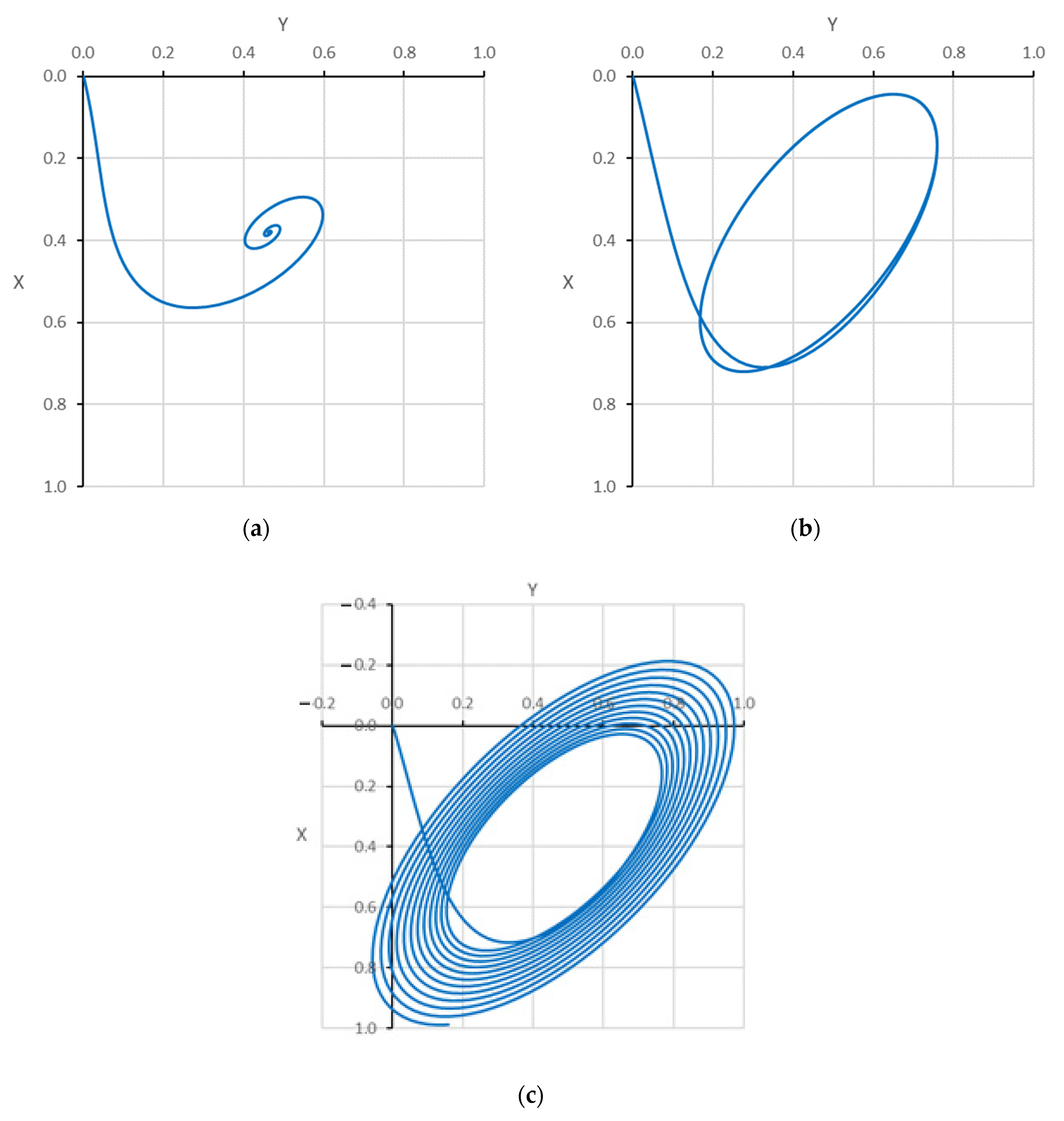
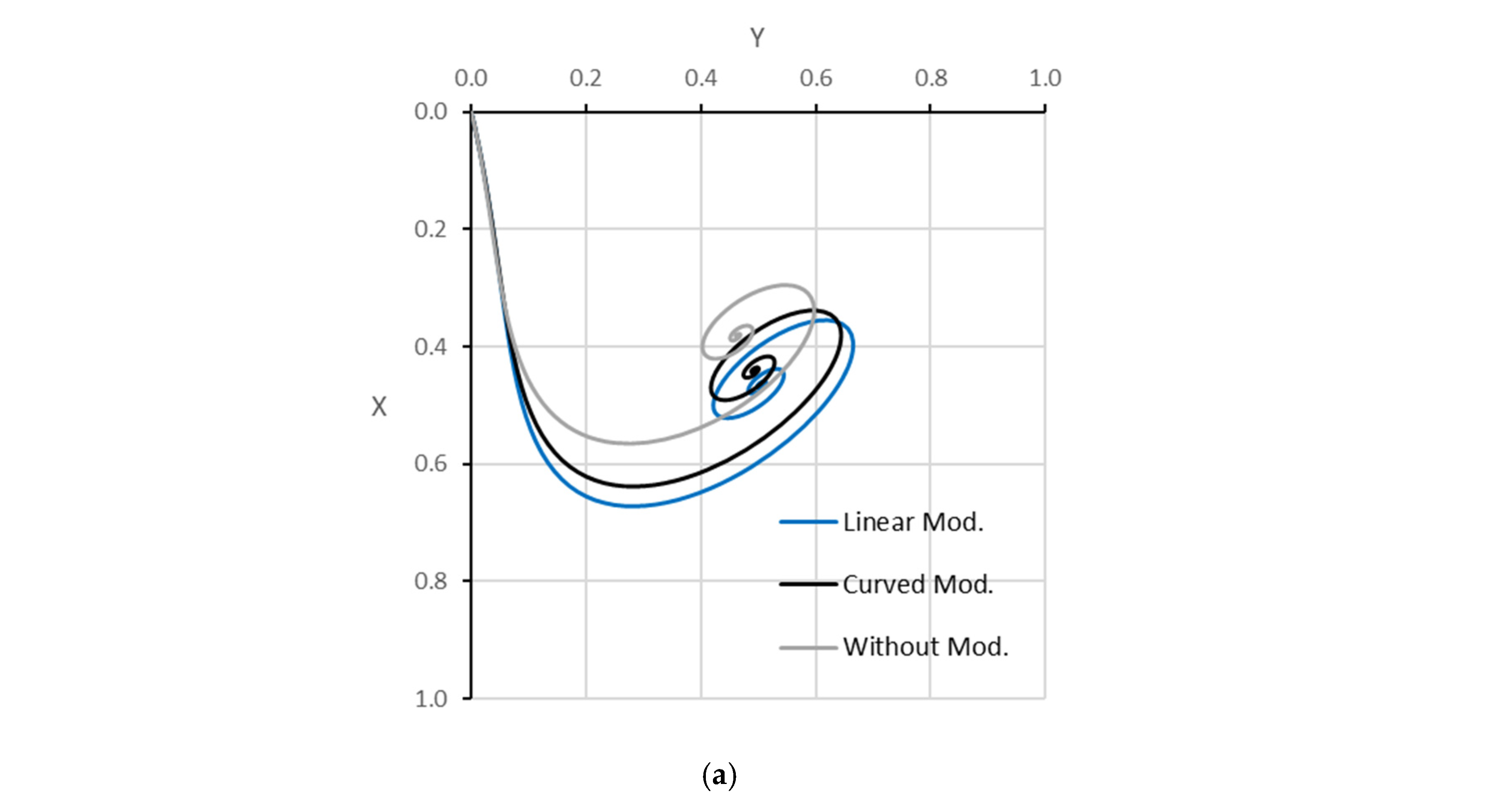
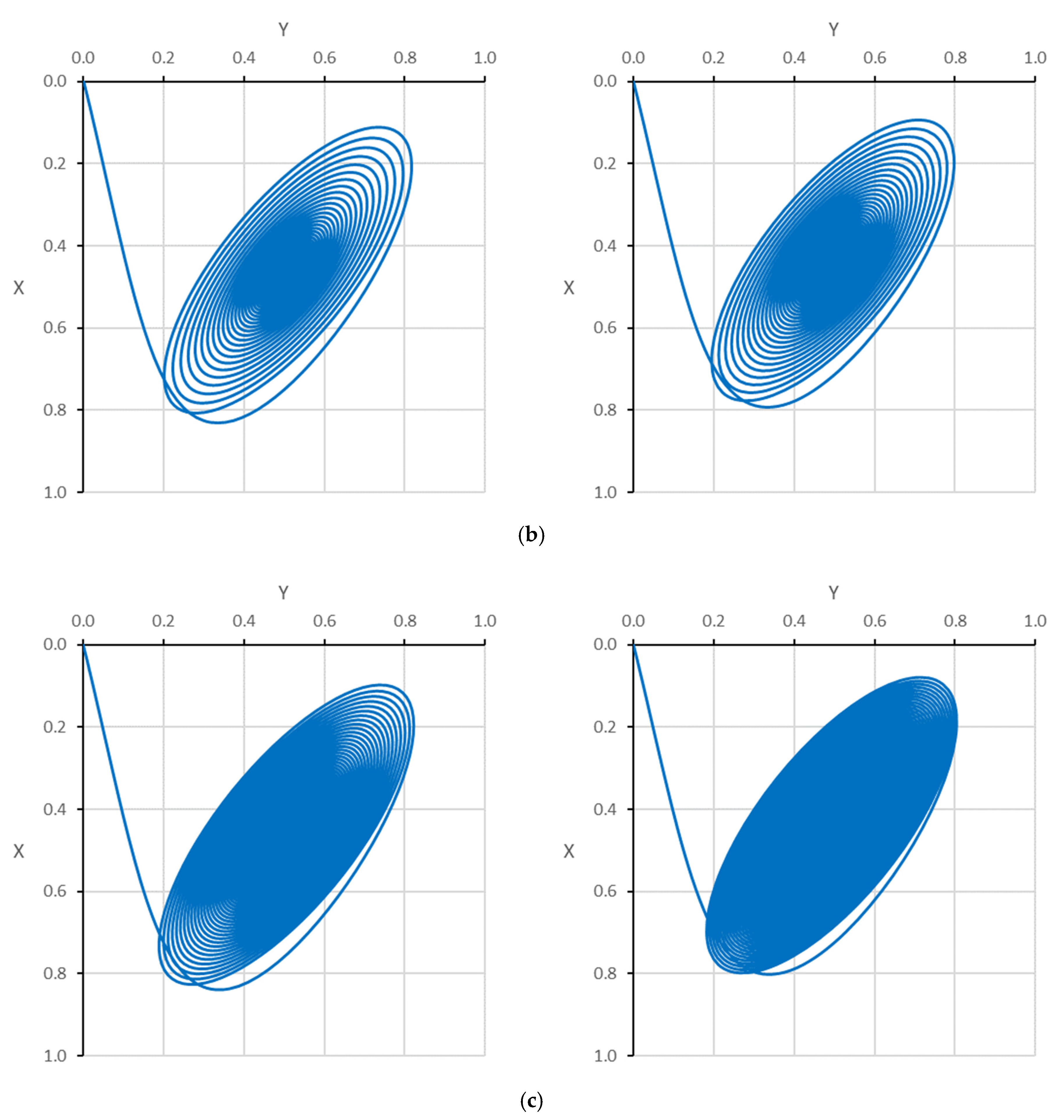
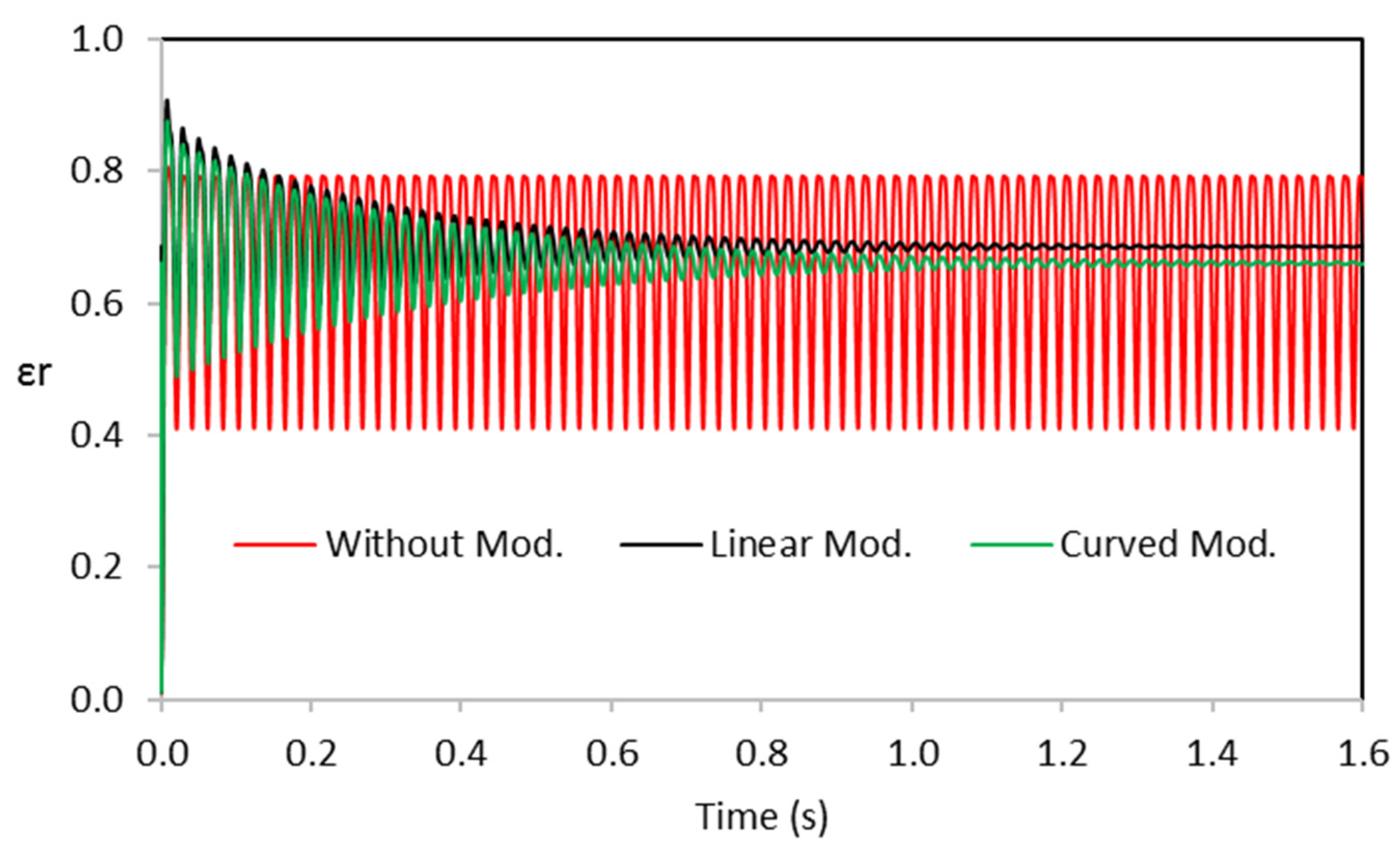
7.4. Effect of Modification on the Journal Trajectory

The journal trajectory during the operation explains the system’s dynamic response to any form of excitation. The operation speed is one of the most vital factors in determining the amplitude of the dynamic response. The journal trajectories will be explained first for the unmodified bearing. Then, the corresponding trajectories of the modified bearing will be explained later for the two forms of modification. Figure 15 illustrates the journal center trajectories for the unmodified system due to position perturbation when $L/D=1.0$ at three different operational speeds, which are half the critical speed, critical speed, and higher than ${\Omega }_{crit}$. Figure 15a shows the journal trajectory at an operating speed of 1.347 (3290 rpm), which is $0.5 {\Omega }_{crit}$. The journal center returns to the steady state position (equilibrium) after a certain period of time, representing the system’s stable condition. Figure 15b shows the corresponding path at an operating speed of 2.694 (6580 rpm), which is ${\Omega }_{crit}$ of the system. It is clear that the journal continues to rotate around the equilibrium position, which represents the critical response of the system where any increase in the operating speed will produce higher amplitude, and the system moves to unstable conditions. Figure 15c illustrates the journal trajectory at an operating speed of 6800 rpm, which is just $1.033 {\Omega }_c$ of the system. The amplitude of the trajectory starts to build up until the shaft’s touches the bush surface. This extremely dangerous situation results from operation under unstable cases, which must be avoided under any circumstances. Extending the range of the operating speed in which the system operates under stable conditions represents a significant enhancement in the design of the considered system, as the operation under severe conditions for a long period of time will certainly impact the designed values of the dynamic characteristics. Modifying the bearing profile helps in this direction in addition to the main improvements in the values of Ho and Po, as explained previously.

Figure 15. The journal center trajectories for the unmodified system, due to position perturbation when $L/D=1.0$ at (a) half the critical speed, (b) critical speed, and (c) greater than ${\Omega }_{crit}$.

Figure 16 shows the dynamic response to shaft perturbation when $L/D=1.0$ for the modified bush under different operating speeds. Figure 16a compares the trajectories when the rotational speed is half ${\Omega }_{crit}$ for the two modification forms in addition to the unmodified bearing. The trajectory of the unmodified system illustrated previously in Figure 15a is repeated here for the purpose of comparison. It can be seen that the journal trajectories of both modified bearings are returned to the equilibrium position with slightly different paths. The curved modification produces a path closer to the unmodified bearing. Figure 16b shows the shaft trajectories of the modified bearings when the operating speed is equal to ${\Omega }_{crit}$ of the unmodified bearing (see Figure 15b for the journal trajectory of the unmodified bearing at critical speed). This figure illustrates that the journal centers return to the steady-state position for both forms of modification in contrast with the continuous rotation around the equilibrium position in the unmodified case. The journal of the modified bearing can operate safely at a speed greater than ${\Omega }_{crit}$ of the unmodified design, as shown in Figure 16c, where the operating speed is 6800 rpm. In this case, the journal center also returns to the steady state position compared with the growing journal amplitude of the unmodified bearing at this speed. Further comparison of the eccentricity ratio variation with time for the unmodified and modified bearings is shown in Figure 17. The operating speed for the results shown in this figure is ${\Omega }_{crit}$ of the unmodified bearing. The eccentricity ratio in the case of unmodified bearing (shown in red) fluctuates continuously around 0.6 (the steady state value) at this speed, while the corresponding eccentricity ratios in both forms of modification reach a steady state value after a period of time. The curved modification produces an eccentricity ratio (shown in green) closer to the steady state value of 0.6. It is worth mentioning that similar behaviors are obtained for the other $L/D$ ratios, which shows a sense of generality in the results.

Figure 16. The journal center trajectories due to position perturbation when $L/D=1.0$ (a) Modified and unmodified bearings at $0.5 {\Omega }_c$ of unmodified bearing, (b) linear (left) and curved (right) modification at ${\Omega }_c$ of unmodified bearing, and (c) linear (left) and curved (right) modification at greater than ${\Omega }_c$ of unmodified bearing.

Figure 17. Comparison between the variation of the eccentricity ratio with time for the unmodified and modified bearings.

8. Conclusions and Remarks

This work investigated the use of two types of bearing profiles on the general performance of rotor bearing systems: linear and curved profiles. The journal bearing considered in this work has a wide range of L/D ratios to represent short, finite-length, and long bearings. The system’s performance was evaluated under the effect of 3D misalignment, which considers both the horizontal and vertical deviations in the axis of the shaft. The numerical solution was based on the finite difference method with the use of the iterative Reynolds boundary condition method. This work examined the effect of misalignment and the new design of the bearing profile on the pressure distribution, the film thickness levels, and the dynamic characteristics of the rotor–bearing system under position perturbation where the 4th-order Runge–Kutta method was used to determine the trajectory of the shaft center. It was found that the variation in the bearing profile, using both types, reduced to a large extent the maximum pressure value and significantly elevated the minimum film of the lubricant, which faced a sharp reduction due to the presence of misalignment. Furthermore, the time response of the modified bearing design using a curved profile was closer to the ideal case in comparison with the linear profile design. The results of this work explain the possibility of enhancing the performance of considered system under severe misalignment conditions, which certainly has a positive effect on the system’s life and reliability.

References

1. Song, X.; Wu, W.; Yuan, S. Mixed-lubrication analysis of misaligned journal bearing considering turbulence and cavitation. AIP Adv. 2022, 12, 015213. [Google Scholar] [CrossRef]
2. Jang, J.Y.; Khonsari, M.M. On the characteristics of misaligned journal bearings. Lubricants 2015, 3, 27–53. [Google Scholar] [CrossRef]
3. Guo, J.; Xiang, G.; Wang, J.; Song, Y.; Cai, J.; Dai, H. On the dynamic wear behavior of misaligned journal bearing with profile modification under mixed lubrication. Surf. Topogr. Metrol. Prop. 2022, 10, 025026. [Google Scholar] [CrossRef]
4. Dufrane, K.; Kannel, J.; McCloskey, T. Wear of steam turbine journal bearings at low operating speeds. J. Tribol. 1983, 105, 313–317. [Google Scholar] [CrossRef]
5. Jang, J.; Khonsari, M.M. On the wear of dynamically loaded engine bearings with provision for misalignment and surface roughness. Tribol. Int. 2020, 141, 105919. [Google Scholar] [CrossRef]
6. Ebrat, O.; Mourelatos, Z.P.; Vlahopoulos, N.; Vaidyanathan, K. Calculation of journal bearing dynamic characteristics including journal misalignment and bearing structural deformation©. Tribol. Trans. 2004, 47, 94–102. [Google Scholar] [CrossRef]
7. Sun, J.; Gui, C.L. Hydrodynamic lubrication analysis of journal bearing considering misalignment caused by shaft deformation. Tribol. Int. 2004, 37, 841–848. [Google Scholar] [CrossRef]
8. Manser, B.; Belaidi, I.; Hamrani, A.; Khelladi, S.; Bakir, F. Performance of hydrodynamic journal bearing under the combined influence of textured surface and journal misalignment: A numerical survey. Comptes Rendus Mécanique 2019, 347, 141–165. [Google Scholar] [CrossRef]
9. Xiang, G.; Han, Y.; Wang, J.; Xiao, K.; Li, J. A transient hydrodynamic lubrication comparative analysis for misaligned micro-grooved bearing considering axial reciprocating movement of shaft. Tribol. Int. 2018, 132, 11–23. [Google Scholar] [CrossRef]
10. Ma, J.; Fu, C.; Zhang, H.; Chu, F.; Shi, Z.; Gu, F.; Ball, A.D. Modelling non-Gaussian surfaces and misalignment for condition monitoring of journal bearings. Measurement 2021, 174, 108983. [Google Scholar] [CrossRef]
11. Jamali, H.U.; Al-Hamood, A. A New Method for the Analysis of Misaligned Journal Bearing. Tribol. Ind. 2018, 40, 213–224. [Google Scholar] [CrossRef]
12. Nikolakopoulos, P.G.; Papadopoulos, C.A. A study of friction in worn misaligned journal bearings under severe hydrodynamic lubrication. Tribol. Int. 2008, 41, 461–472. [Google Scholar] [CrossRef]
13. Nacy, S.M. Effect of Chamfering on Side-Leakage Flow Rate of Journal Bearings. Wear 1997, 212, 95–102. [Google Scholar] [CrossRef]
14. Fillon, M.; Bouyer, J. Thermohydrodynamic Analysis of a Worn Plain Journal Bearing. Tribol. Int. 2004, 37, 129–136. [Google Scholar] [CrossRef]
15. Strzelecki, S. Operating Characteristics of Heavy Loaded Cylindrical Journal Bearing with Variable Axial Profile. Mater. Res. 2005, 8, 481–486. [Google Scholar] [CrossRef]
16. Chasalevris, A.; Dohnal, F. Enhancing Stability of Industrial Turbines Using Adjustable Partial Arc Bearings. J. Phys. Conf. Ser. 2016, 744, 12152. [Google Scholar] [CrossRef]
17. Ren, P.; Zuo, Z.; Huang, W. Effects of axial profile on the main bearing performance of internal combustion engine and its optimization using multiobjective optimization algorithms. J. Mech. Sci. Technol. 2021, 35, 3519–3531. [Google Scholar] [CrossRef]
18. Allmaier, H.; Offner, G. Current Challenges and Frontiers for the EHD Simulation of Journal Bearings: A Review; SAE International: Warrendale, PA, USA, 2016. [Google Scholar] [CrossRef]
19. Atlassi, K.; Nabhani, M.; El Khlifi, M. Ferrofluid squeeze film lubrication: Surface roughness effect. Ind. Lubr. Tribol. 2023, 75, 133–142. [Google Scholar] [CrossRef]
20. Chasalevris, A.; Sfyris, D. Evaluation of the Finite Journal Bearing Characteristics, Using the Exact Analytical Solution of the Reynolds Equation. Tribol. Int. 2013, 57, 216–234. [Google Scholar] [CrossRef]
21. Hamrock, B.J. Fundamentals of Fluid Film Lubrication; McGraw-Hill Inc.: New York, NY, USA, 1991. [Google Scholar]
22. Harnoy, A. Bearing Design in Machinery: Engineering Tribology and Lubrication, 1st ed.; Marcel Dekker Inc.: New York, NY, USA; Basel, Switzerland, 2002. [Google Scholar]
23. Feng, H.; Jiang, S.; Ji, A. Investigation of the Static and Dynamic Characteristics of Water-Lubricated Hydrodynamic Journal Bearing Considering Turbulent, Thermo-hydrodynamic and Misaligned Effects. Tribol. Int. 2019, 130, 245–260. [Google Scholar] [CrossRef]
24. Nicholas, J.C. Hydrodynamic journal bearings, types, characteristics and applications. In Proceedings of the 20th Annual Meeting, Valencia, Spain, 8–12 July 1996; The Vibration Institute: Willowbrook, IL, USA, 2016; pp. 79–100. [Google Scholar]
25. Lund, J.W.; Thomsen, K.K. A Calculation Method and Data for the Dynamic Coefficients of Oil-Lubricated Journal Bearings; ASME: New York, NY, USA, 1978. [Google Scholar]
26. Someya, T. Journal Bearing Databook; Springer: Berlin/Heidelberg, Germany, 1989. [Google Scholar]
27. Tieu, A.K.; Qiu, Z.L. Stability of Finite Journal Bearings—From Linear and Nonlinear Bearing Forces. Tribol. Trans. 1995, 38, 627–635. [Google Scholar] [CrossRef]
28. Shi, Y.; Li, M. Study on nonlinear dynamics of the marine rotor-bearing system under yawing motion. J. Phys. Conf. Ser. 2020, 1676, 012156. [Google Scholar] [CrossRef]
29. D’Amato, R.; Amato, G.; Wang, C.; Ruggiero, A. A Novel Tracking Control Strategy with Adaptive Noise Cancellation for Flexible Rotor Trajectories in Lubricated Bearings. IEEE/ASME Trans. Mechatron. 2021, 27, 753–765. [Google Scholar] [CrossRef]
30. Atlassi, K.; Nabhani, M.; El Khlifi, M. Rotational viscosity effect on the stability of finite journal bearings lubricated by ferrofluids. J. Braz. Soc. Mech. Sci. Eng. 2021, 43, 548. [Google Scholar] [CrossRef]