Techno-Economic Feasibility Study of a 1.5 MW Grid-Connected Solar Power Plant in Bangladesh

Abstract

This study addresses the pressing energy constraints in nations like Bangladesh by proposing the implementation of photovoltaic (PV) microgrids. Given concerns about environmental degradation, limited fossil fuel reserves, and volatile product costs, renewable energy sources are gaining momentum globally. Our research focuses on a grid-connected solar PV system model at Char Jazira, Lalpur, Natore, Rajshahi, Bangladesh. Through PVsyst 7.1 simulation software, we assess the performance ratio (PR) and system losses, revealing an annual solar energy potential of 3375 MWh at standard test condition (STC) efficiency. After considering losses, the system generates 2815.2 MWh annually, with 2774 MWh exported to the grid. We analyze an average PR of 78.63% and calculate a levelized cost of energy (LCOE) of 2.82 BDT/kWh [1 USD = 110 BDT]. The financial assessment indicates a cost-effective LCOE for the grid-connected PV system, with an annual gross income of 27,744 kBDT from selling energy to the grid and operating costs of 64,060.60 BDT/year. Remarkably, this initiative can prevent 37,647.82 tCO₂ emissions over the project’s 25-year lifespan.

1. Introduction

In Bangladesh, fossil fuels presently dominate energy production, accounting for 99% of the total [1]. However, the country has established challenging renewable energy targets for 2030 and 2040, mandating major time and financial commitments [1]. To accomplish these goals, solar energy is poised to be extremely important [1]. As the world actively seeks sustainable energy solutions, solar power has emerged as a prominent player [2]. Grid-connected solar power plants are a focus of efforts worldwide to cut carbon emissions and switch to cleaner electricity sources since they can capture a lot of sunshine with little harm to the environment [3,4].

This study’s main goal is to evaluate the feasibility of building a 1.5 MW solar power plant in Lalpur, Natore, Bangladesh, while taking into account its integration with the current grid system. The evaluation utilizes the robust simulation capabilities of the PVsyst program. Notably, Bangladesh experiences an average annual increase in energy demand of 4.68%, attributed to a burgeoning population and an improving economy [1]. Like many nations, Bangladesh faces the dual challenge of meeting escalating energy demands while mitigating greenhouse gas emissions [5]. Interest in the development of solar power has increased as a result of the country’s adherence to the Paris Agreement and desire to increase the proportion of renewable energy in its energy mix [6]. Given Bangladesh’s abundant solar irradiance, there is a significant opportunity to harness solar energy, bolstering the nation’s energy security and aligning with its environmental objectives [7]. Aligned with the Paris Agreement and a commitment to increasing renewable energy in its mix, Bangladesh sees a substantial opportunity to harness its abundant solar irradiance. The study emphasizes the importance of renewable energy, especially solar power, to enhance the nation’s energy security and align with environmental objectives.

The goal of this study is perfectly aligned with the concept of a positive energy district (PED) whose goal is to attain a net positive energy balance. This means that it produces more energy from sustainable technologies, such as wind turbines and solar panels, than it consumes for infrastructure, buildings, and transportation. Greenhouse gas emissions are decreased and a district’s dependency on fossil fuels is lessened by incorporating solar power into its energy mix. This makes the district more environmentally friendly since it is in line with sustainability and environmental aims [8,9,10,11]. Local energy production is the goal of positive energy districts. By generating electricity locally, solar power plants help to achieve this objective. This improves energy independence and lessens reliance on centralized power systems. There can be significant cost reductions using solar electricity. Positive energy districts can drastically lower their energy costs by producing their own electricity. It is also possible to resell extra energy to the grid to generate revenue or offset energy expenses. A district’s energy supply can be made more resilient with the use of solar electricity. Solar panels can continue to produce electricity even when the grid is down, acting as a dependable source of power [12,13,14,15]. A PED should incorporate solar power with other sustainable technology, including energy-efficient buildings, sophisticated energy-storage systems, and smart grid management, to maximize these advantages. A district can therefore aim to achieve net positive energy and create a more robust, cost-effective, and sustainable energy ecology [16,17,18,19].

By establishing the 1.5 MW solar power plant, a district or city can become more self-sufficient in energy generation. In a broader context, the effect of such a renewable energy project could lead to the creation of a district producing more energy than it consumes, thereby aligning with the principles of a positive energy district. The feasibility study in the research work includes technical and economic assessments, such as evaluating the technology, costs, and benefits of implementing the solar power plant. A similar methodology is crucial in planning and executing projects within a positive energy district, as they require a comprehensive analysis of various energy sources, consumption patterns, and cost-effectiveness. A thorough techno-economic feasibility analysis is essential before moving forward with the development of a solar power plant. These analyses provide a complete evaluation of the viability of the proposed project, taking into account technical, economic, and environmental factors [20,21].

The technical factors are taken into account as follows. (i) Location and site suitability: The location of the solar power plant is crucial. Factors like solar irradiance, weather patterns, available land, topography, and proximity to the grid infrastructure are evaluated. (ii) Technology and equipment selection: Assessing the appropriate solar panel technology, inverters, racking systems, and other equipment is important, considering efficiency, durability, and compatibility with the site. (iii) System design and engineering: Designing the layout of the solar array, considering factors like orientation, tilt angle, and shading analysis is crucial to optimize energy production. (iv) Grid integration and interconnection: Evaluating the compatibility of the solar power plant with the existing grid infrastructure is essential to ensure proper interconnection and grid stability. (v) Maintenance and operations: Considering the maintenance requirements, operational procedures, and lifecycle costs is necessary to ensure smooth operations and optimal performance over the plant’s lifetime.

The economic factors are described as follows. (i) Cost analysis: The initial capital costs for equipment, installation, land, and other associated expenses are estimated. Additionally, ongoing operational and maintenance costs are also considered. (ii) Return on investment and financial viability: Calculating the projected revenue from electricity sales, considering feed-in tariffs or power purchase agreements, and analyzing the payback period and overall return on investment are important for economic feedback. (iii) Incentives and financing: Available incentives, subsidies, tax credits, and financing options are evaluated to determine the financial feasibility of the project. (iv) Economic risks: Risks associated with market fluctuations, changes in regulations, and potential cost escalations are assessed that could impact the financial viability of the project.

The environmental factors are considered as follows. (i) Greenhouse gas emissions: The reduction in greenhouse gas emissions is achieved by generating solar power compared to conventional fossil fuel-based power generation. (ii) Land use and ecosystem impact: The impact on local ecosystems, land use, and potential mitigations are evaluated for minimizing disruption or enhancing biodiversity in the area. (iii) Resource consumption: The environmental impact of manufacturing solar panels is assessed, including energy and material inputs, and recycling or disposal measures are considered at the end of their life cycle. (iv) Social and community impact: The social aspects such as community acceptance, job creation, and local economic benefits derived from the solar power plant are considered.

By evaluating the technical, economic, and environmental aspects, decision-makers can make well-informed choices regarding project implementation. Additionally, techno-economic analyses shed light on the potential risks, challenges, and opportunities associated with the project. A study at Pakistan’s Islamia University in Bahawalpur advocates for the installation of a grid-connected PV system, emphasizing its effectiveness and ecological benefits [22]. This solar-powered system produces 4908 MWh each year, which is comparable to 147,600 teak trees planted during a lifetime or 15,369.3 kg of coal saved per day. The study’s objective is to assist with the creation, evaluation, implementation, and upkeep of new grid-connected systems across numerous places [22]. Afghanistan faces a challenging energy situation, relying on electricity imports and incurring significant costs [23]. To address this, the government plans to generate 5000 MW of renewable energy by 2032, with a focus on 1500 MW of solar projects. Afghanistan’s Daikundi province offers the best sunlight for solar energy production, as shown by a 700 kWp grid-connected solar power plant that was tested using the PVsyst program [23]. The effectiveness of a standalone solar PV system concerning the load requirements at the mechanical department office at Bikaner Engineering College is the subject of another study [24]. The study reveals an average yearly energy need of 1086.24 kWh, with the solar panel providing 1143.6 kWh. Multiple losses contributed to the system’s reduced power capacity, with variations in performance ratio throughout the year [24].

In another research study [25], the viability of a 200 KWp on-grid monocrystalline silicon solar project in Dubai was assessed using the PVsyst program. The system exhibited an impressive yearly performance ratio of 81.67%. From its 32 parallel strings and 22 series modules, the solar facility generated 352.6 MWh annually, achieving an energy output of 1757 kWh/KWp per year. This study further offered detailed loss estimates for the entire year, providing valuable insights into the system’s performance [25]. Another article focused on the viability of a solar PV plant in Pune, India, utilizing a 250 KWp Si-poly photovoltaic facility as the subject [26]. To model the plant, which consisted of 310 Wp modules coupled to 65 strings and 42 string inverters, the study used PVsyst 7.2 software and Meteonorm 8.0 data. Several tests were carried out to establish the best angle for power generation, taking into account things like incidence radiation, performance ratio, and grid input energy [26]. Additionally, a study used PVsyst software to analyze a 20MW grid-connected solar facility in Devdurga, Karnataka, India [27]. The analysis provided insights into performance trajectories and geographical positioning, predicting a 110-acre area with a remarkable 76.28% performance ratio. The study also examined the system’s behavior concerning tilt and orientation, further enriching our understanding of solar plant dynamics [27].

In a notable study [28], the grid connected photovoltaic array system, which is intended to produce 15 kWp at STC, was the main focus. The study carefully looked into several factors, including system output, output power losses, performance ratio, output energy, PV module output, field type adjustment, power distribution curves, temperature distribution, and module connection in string design [28]. Furthermore, another research effort involved the design and simulation of a 60 kWp solar power plant for a rural area in Uttar Pradesh, India, utilizing PVsyst software version 7.2.2. The analysis considered seasonal tilt angles and conducted a comprehensive performance study [29]. A separate research paper [30] delved into a study of a 1 MW photovoltaic plant located in Morocco’s northern zone. The study utilized PVsyst software to evaluate the plant’s performance, making comparisons among solar energy production at different sites. This study underscored the critical need for accurate predictions of system efficiency in renewable energy systems [30]. PVsyst simulation software was employed in yet another study [31], where the main goal was to build and simulate a hybrid photovoltaic system for a system of energy-efficient street lighting. The system comprised 16 Narada batteries, 13 series-connected modules, and 4 parallel strings. The modeling showed a yearly energy output of 26.68 MWh overall and an annual energy production of 1283 kWh/KWp specifically. Notably, the study highlighted performance ratios and battery cycle conditions, providing valuable insights into system behavior. In a different research endeavor [32], a 5 MW solar power project in Afghanistan’s Ghor region was planned and simulated. The plant incorporated a 5300 kW Growatt converter type and 6399 KWp STP-320 W PV module. Various modeling tools, including PVsyst, PVGIS, and HOMER, were utilized to evaluate solar renewable energy sources. The findings showcased annual energy generation variations among the modeling tools, emphasizing the importance of accurate simulation for efficient planning.

Despite the existing studies utilizing PVsyst and exploring solar power plant designs and financial aspects, there is a research gap in conducting a comprehensive analysis encompassing detailed losses, financial analysis, cost-effectiveness, and carbon balance collectively. Additionally, previous works have not sufficiently addressed the potential challenges, risks, and mitigation strategies associated with the implementation of solar power plants. Our study bridges these research gaps by introducing a novel approach to solar energy project assessment, focusing on the specific site of Lalpur, Natore, Bangladesh. The geographical specificity of Char Jazira, a riverine island in the floodplains of the Jamuna River, is highlighted, emphasizing its ideal characteristics for a solar project. The inclusion of detailed meteorological data, covering parameters such as global horizontal irradiance, temperature, wind velocity, Linke turbidity, and relative humidity, adds depth to the study. The comprehensive techno-economic feasibility assessment, utilizing PVsyst software for modeling, brings a nuanced understanding of the solar power plant’s viability. Performance analysis reveals seasonal variations and the environmental impact is quantified, emphasizing a significant reduction in carbon emissions. The study’s economic viability metrics, including a quick payback period, underscore the practicality of the proposed solar project. In essence, the paper offers a holistic exploration of solar energy potential, integrating geographical, meteorological, economic, and environmental considerations, making notable contributions to sustainable energy solutions.

In this study, we have used the potent PVsyst program to model the operation of a 1.5 MW grid-connected solar power plant in Lalpur, Natore. PVsyst is highly esteemed for its capacity to model PV systems under varying conditions encompassing solar irradiance, temperature, shading, and system configuration [33]. The software enables accurate predictions of energy generation, performance ratios, and financial metrics, rendering it an invaluable tool in the feasibility assessment of solar projects [34]. However, a collective and detailed analysis, including losses, financial aspects, cost-effectiveness with a simple payback period, and carbon balance, has not been previously conducted in the mentioned research and studies.

We intend to develop the solar power plant layout after assessing the project site’s solar resource potential and climate. Important aspects to take into account are the panel orientation, tilt angle, and shading analysis [35,36]. With the aid of the PVsyst program, we intend to simulate the energy generation profile of the solar power plant under various conditions. This simulation will help to estimate key financial metrics such as the LCOE, payback period, and ROI, enabling a comprehensive assessment of the project’s economic viability [24]. Additionally, we want to pinpoint any obstacles, dangers, and suitable countermeasures related to the construction of the solar power plant [37,38,39].

This study is divided into several sections, each of which deals with a different component of the techno-economic feasibility assessment. These sections include an evaluation of the solar resource, plant design and simulation, financial analysis, and a discussion of findings. Through this structured approach, we aim to attain a comprehensive understanding of the project’s viability and potential benefits, empowering informed decision-making in the pursuit of sustainable energy solutions.

2. Location and Data

2.1. Project Site Selection

The chosen project site is located in Lalpur, Natore, Rajshahi, Bangladesh, specifically known as Char Jazira. The geographical coordinates for this location are 24.0900° N latitude, 88.5800° E longitude, and an altitude of 22 m above sea level. The time zone in this region is UTC+6. In Bangladesh, a ‘char’ typically denotes a riverine island or sandbar that forms within the braided river systems, shaped by the dynamics of sedimentation and erosion in the river. The specific location for this project, Char Jazira, fits this description. Char Jazira is positioned in the floodplains of the Jamuna River, a major river in Bangladesh. The land is state-owned, and due to its nature as a riverine island, it is devoid of tree shadows, making it ideal for a solar project. The incident solar irradiation in this area is notably high. The location of Char Jazira, Lalpur, in Bangladesh has been shown in Figure 1 and Figure 2 using a pinned location and red color marked area, respectively, from Google Maps.

The average annual rainfall in Lalpur, Natore, Bangladesh, is 2200 mm (86.6 inches). The wettest months are June, July, and August, receiving an average rainfall of 300 mm (11.8 inches) each. On the other hand, the driest months, namely December, January, and February, witness an average rainfall of 50 mm (2.0 inches) each. Lalpur in Natore, Bangladesh, observes the lowest rainfall during these months.

Considering the above information regarding the project site, there is huge potential for one power plant in the location chosen for the solar power plant, and it must contribute to the country’s crucial grid electricity. Thus, the analysis of the project on that site can be considered notable and novel.

2.2. Meteorological Data

PVsyst software relies primarily on solar irradiance data for the accurate modeling of solar photovoltaic (PV) systems. In addition to solar irradiance data, meteorological data are also incorporated to enhance the precision of system modeling [40,41,42]. The following

Table 1. Collected and applied meteorological data.

Month	Global Horizontal Irradiance (kWh/m2/mth)	Diffuse Horizontal Irradiance (kWh/m2/mth)	Temperature (Degree Celcius)	Wind Velocity (m/s)	Linke Turbidity	Relative Humidity (%)
January	122.3	54.1	17.4	0.79	6.377	77.6
February	132.6	60.3	21.5	0.91	5.946	70.6
March	174.6	78.3	26.5	1.2	6.316	64.6
April	182.5	88.7	29.1	1.4	7	71.3
May	190	100.7	30.3	1.1	7	71.4
June	155.3	99.9	29.5	0.98	7	79.9
July	145.1	99.2	29.2	0.88	5.772	80.9
August	145.8	90.6	29	1.3	5.18	83.1
September	139.4	74.2	27.9	1.2	5.29	86.5
October	136	72.5	27	0.8	5.7	81.7
November	127.8	54	23.1	0.6	6.589	78.4
December	122.7	50.2	18.7	0.6	6.948	79.1

shows the key meteorological parameters collected and needed for the software simulation of the solar power plant.

2.2.1. Solar Irradiance

Solar irradiance data is essential for PVsyst software to compute a PV system’s energy production accurately. This data includes:

-

Global horizontal irradiance (GHI): Total solar energy, including both direct and diffuse solar radiation, that is received on a horizontal portion of the Earth’s surface. GHI, which is measured in watts per square meter (W/m²), is an important aspect to consider when assessing the solar energy potential of a site [41,43].

-

Direct normal irradiance (DNI): Solar radiation that strikes a surface perpendicular to the sun’s rays. DNI is the amount of sunlight that enters the Earth straight from the sun, unaffected by air absorption or scattering. It is essential for applications and concentrated solar power (CSP) systems that need direct sunshine. Watts per square meter (W/m²) are commonly used to measure DNI [44,45,46].

-

Diffuse horizontal irradiance (DHI): Aside from direct sunlight, solar radiation is received from the sky. DHI is made up of solar energy that is reflected or dispersed and diffusely reaches the surface of the Earth. It is crucial for solar energy applications since it is measured on a horizontal surface, especially for PV systems that may take in both direct and diffuse sunlight. DHI can also be calculated in W/m² [44,47].

Understanding and utilizing these meteorological parameters in the PVsyst software is crucial for the precise modeling and assessment of solar energy systems. Applied GHI and DHI values from Table 1 are plotted in Figure 3.

2.2.2. Temperature

The performance of PV modules is greatly influenced by the ambient temperature. Temperature information is necessary for PVsyst software to accurately analyze the attributes of PV modules. The electrical characteristics of the PV modules can be determined with the use of these temperature data. In actuality, hot, bright days with little breeze tend to have higher operating temperatures for PV modules. A PV module’s temperature is predicted by the nominal operating cell temperature (NOCT), a standardized rating system, under a variety of parameters, such as 20 °C ambient temperature, 800 W/m² of solar energy, and 1 m/s of wind speed. It is essential to comprehend a PV module’s temperature because it has a significant impact on its electrical properties [48].

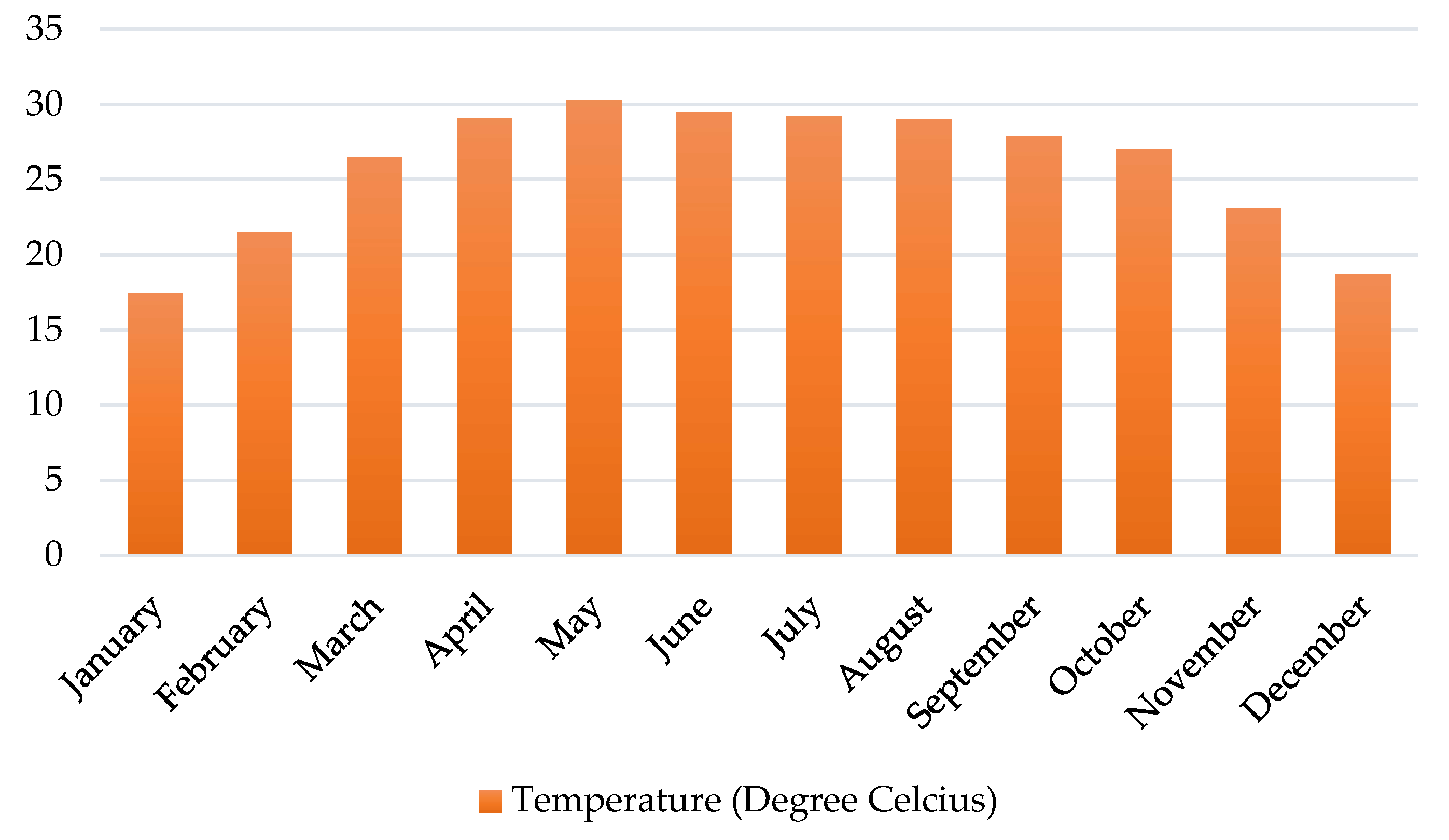
A detrimental effect of temperature arises on a PV module’s efficiency. The energy band gap of the semiconductor material narrows with temperature, requiring less energy to produce a free electron-hole pair, which results in a decrease in efficiency. As a result, a PV module’s power production decreases as temperature increases. The temperature coefficient of power (Pmax), which is often stated as a percentage per degree Celsius (°C), measures this decrease in power output caused by an increase in temperature [49]. Understanding how temperature changes affect a PV module’s performance requires an understanding of the temperature coefficient of power. Applied temperature values in degrees Celsius (°C) from Table 1 for the software simulation are plotted in Figure 4.

2.2.3. Wind Velocity

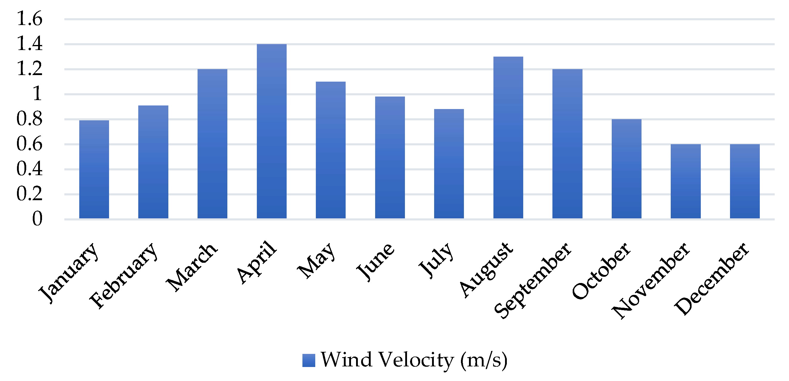
Wind velocity, or wind speed, significantly influences the performance of PV modules by affecting their operating temperature and cooling mechanisms. Accurate wind speed data are crucial for the PVsyst software to estimate the cooling effect on module performance and simulate its impact on energy production. Wind speed plays a beneficial role in solar power generation from panels. It aids in cooling the solar panels, consequently improving their efficiency. As solar panels become hotter, their efficiency tends to decrease. Wind helps dissipate this heat, maintaining or even enhancing the panel’s performance. Wind also aids in removing dirt and debris from solar panels’ surfaces, increasing their effectiveness. The electricity production of solar panels can increase by up to 20% when there is wind. The precise rise, however, relies on several variables, including the surrounding temperature, sun irradiation, and the type of solar panel being utilized. In general, higher wind speeds cause solar power generation to rise more quickly. The rise in power production does level off at a certain point, though. This is because the cooling effect of wind becomes less significant as the wind velocity continues to increase [50,51].

Understanding and incorporating wind speed data into simulations is critical for accurately assessing the impact of wind on solar panel efficiency and optimizing solar power generation. In Figure 5, the values of wind velocity from Table 1 collected for the location for every month of a certain year are plotted.

2.2.4. Linke Turbidity

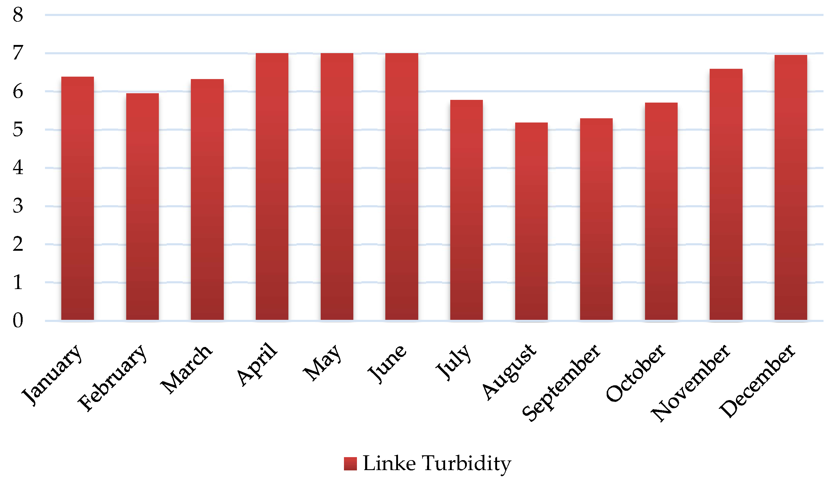
In the context of solar energy modeling, the Linke turbidity coefficient serves as an atmospheric parameter that provides insights into water vapor concentrations and aerosols. While the clear sky model primarily uses location coordinates (latitude, longitude, and altitude), the Linke turbidity coefficient can introduce slight alterations. This coefficient typically ranges from 2.0, indicating a very dry and clear sky, to 5 or 6, indicating a humid and potentially polluted environment. A common default value used for many sites is 3.5 [52,53]. Turbidity, in a broader sense, characterizes the cloudiness or haziness of a liquid caused by numerous small suspended particles, including dust, sediment, organic materials, and plankton in water. Turbidity has a considerable impact on the amount and distribution of solar radiation that reaches solar PV panels or solar thermal collectors in the field of solar energy production.

Turbidity in the atmosphere can absorb and scatter light, reducing the amount of direct and diffuse solar irradiance that reaches solar panels. This decrease in solar irradiance ultimately diminishes the overall energy output of PV panels. Turbidity’s impact is evident in the scattering of sunlight, potentially increasing the diffuse solar radiation component while decreasing direct solar radiation due to scattering. Certain solar energy systems, particularly those adept at capturing diffuse sunlight effectively, can benefit from this shift. Additionally, turbidity may appear as debris, dust, or dirt adhering to the PV panel’s surface. The buildup of these particles reduces direct sunlight’s ability to reach the solar cells, which has an impact on the PV system’s effectiveness and power generation [54]. The performance of solar panels must be maximized, which means keeping them clean and removing as many of these impediments as possible. The values of Linke turbidity from Table 1 are plotted in Figure 6.

2.2.5. Relative Humidity

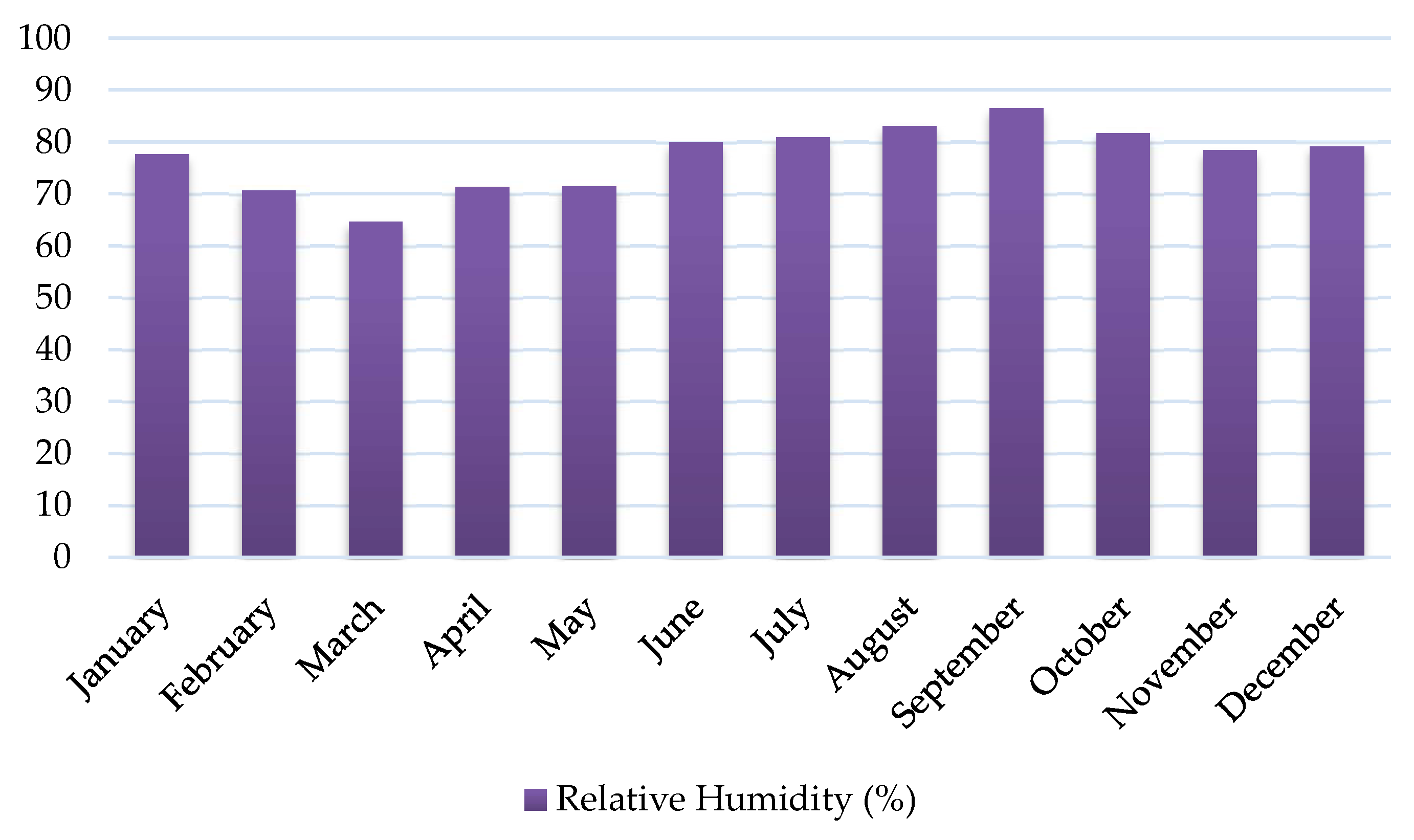
A measurement known as relative humidity (RH) expresses the amount of moisture in the air in relation to the maximum amount of moisture the air may contain at a specific temperature. Its relevance for solar radiation and PV panel efficiency—two important factors impacting solar power generation—is stated as a percentage. The PV module temperature and efficiency are both significantly influenced by relative humidity. It has an impact on the module’s electrical properties, which may therefore have an impact on energy output. The software’s ability to correctly assess these effects depends on accurate input of relative humidity data.

In terms of solar radiation, relative humidity directly affects the amount of direct and diffuse solar radiation reaching solar panels. Cloud cover and a rise in atmospheric water vapor are frequently correlated with a higher relative humidity. Clouds can reflect and absorb sunlight, reducing the amount of direct solar irradiance that reaches solar panels and, as a result, reducing the energy output. Elevated relative humidity levels, often associated with increased cloud cover, lead to a higher proportion of diffuse solar radiation. Despite the reduction in direct sunlight due to cloud cover, diffuse radiation still contributes to the overall energy production of solar panels.

Relative humidity is closely intertwined with temperature. As temperature increases, the air can retain more moisture, resulting in a lower relative humidity for the same absolute moisture content. High temperatures, usually linked with low relative humidity, can enhance PV panel efficiency by reducing resistive losses within the solar cells. Regions with a high moisture content or coastal areas, often characterized by higher humidity levels, can experience dust and dirt accumulation on solar panels. Regular cleaning and maintenance of solar panels are crucial to ensure that accumulated dirt does not obstruct sunlight absorption and impact energy production [55,56]. Keeping the panels clean optimizes their performance and, in turn, the overall solar power generation efficiency. The collected and applied values of relative humidity from Table 1 are plotted in Figure 7.

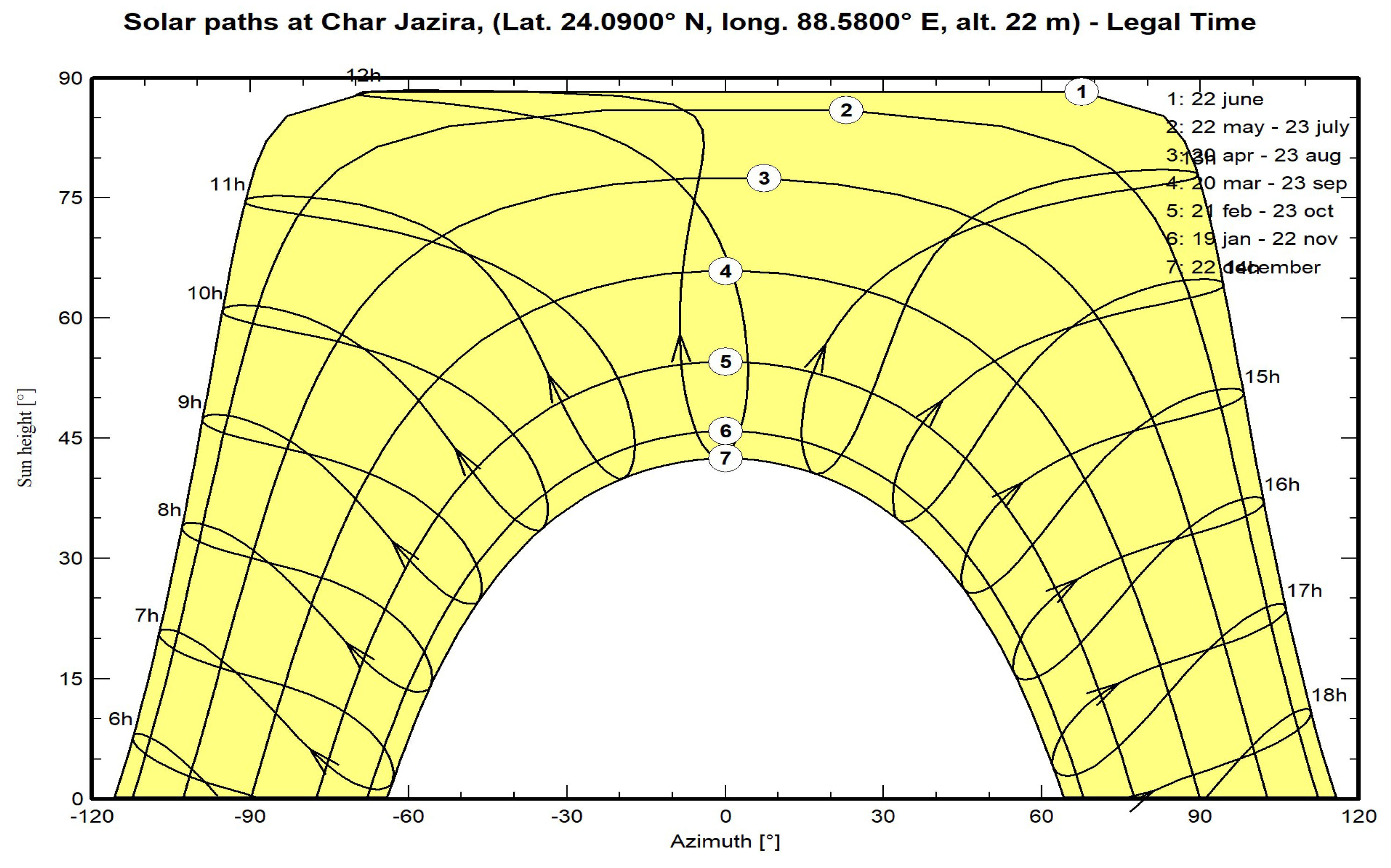
2.3. Sun Paths Diagram

Sun path analysis is crucial for determining the solar irradiation and shading conditions at a specific location over a given period. PVsyst makes use of solar geometry computations to determine the sun’s position in relation to the site and time of interest. It precisely determines the sun’s position throughout the year by taking into account variables like latitude, longitude, time zone, and date. The software can generate detailed graphical representations of the sun’s path, including azimuth and sun height angles [57], as shown in Figure 8 for the selected location of Char Jazira, Lalpur. This graphic of solar paths shows the sun’s daily position in the sky, as well as the seasons. PVsyst assists users in assessing the effects of shadowing, figuring out the best tilt and orientation for solar panels, and analyzing the overall solar energy potential at a particular site by visualizing the sun’s path [58].

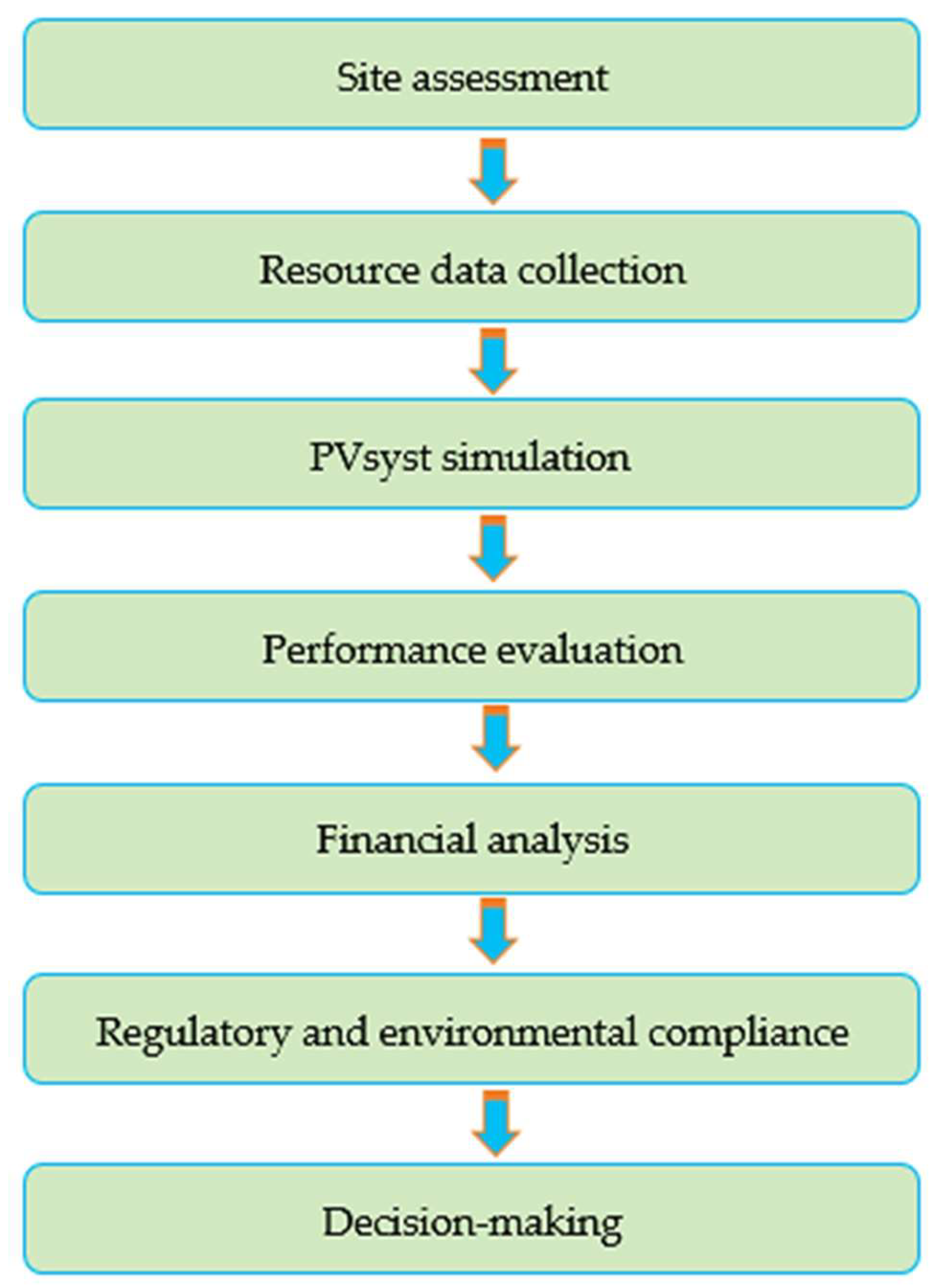
3. Methodology

The steps of methodology for this research work are depicted in Figure 9 as a flowchart. The steps in the flowchart are described as follows. Site assessment: An important stage in guaranteeing the success of a solar project is to carry out an on-site assessment of the solar plant location in Lalpur, Natore, to obtain information on solar irradiance, shading analyses, weather patterns, and topographical factors. This information is essential for precisely estimating the region’s solar potential and adjusting the layout and positioning of solar panels to increase their effectiveness and sustainability. Additionally, the evaluation will help in identifying potential challenges or limitations associated with the location that may need to be addressed during the planning and implementation phases of the solar project.

Resource data collection: After the site assessment, collecting historical solar irradiance, meteorological data (temperature, wind velocity, Linke turbidity, relative humidity), and PV field orientation (tilt, azimuth) for the region to accurately model the plant’s performance is essential for designing and operating a reliable and efficient solar power plant.

PVsyst simulation: Assessing the site and then giving input to PVsyst by using collected data to simulate the solar power plant’s energy production, considering various factors like module type, array layout, inverter specifications, and system losses, allows for a precise and detailed projection of the plant’s potential output. This simulation aids in optimizing the solar power system’s configuration, ensuring it is tailored to the specific conditions of the Lalpur, Natore, location and can operate at peak efficiency, thus maximizing energy generation and overall performance.

Performance evaluation: After PVsyst simulation, the results obtained from PVsyst are crucial to assess the plant’s annual energy yield, capacity factor, and performance ratio, considering local climatic conditions and system parameters. This evaluation provides valuable insights into the solar power plant’s overall efficiency and productivity, allowing for informed decisions on potential optimizations or adjustments needed to enhance energy output and ensure the system operates at its highest capacity throughout the year, factoring in the specific weather patterns and environmental variables of the region.

Financial analysis: Evaluating the performance, and the estimation of project costs, including equipment procurement, installation, grid connection, operation, and maintenance, is essential. Calculation of the LCOE and payback period is crucial to evaluate economic viability, providing key financial indicators that help stakeholders to assess the long-term sustainability and profitability of the solar power project. These assessments ensure that the investment aligns with the financial goals and objectives of the project, enabling informed decision-making and potential adjustments to the project plan to achieve a feasible and economically sound solar power venture.

Regulatory and environmental compliance: Evaluation of legal and regulatory requirements for solar installations in Bangladesh is imperative, ensuring compliance with permits, grid codes, and environmental standards. Adhering to these guidelines not only ensures the legality and smooth operation of the solar power plant but also upholds environmental sustainability and safety standards set by the governing bodies. Comprehensive compliance guarantees that the solar project aligns with the country’s policies, fostering a sustainable and responsible approach to solar energy deployment within the regulatory framework of Bangladesh.

Decision-making: Taking into account both technical and economic factors, based on the detailed analysis, an informed decision has to be made on the feasibility of building the 1.5 MW grid-connected solar power plant. Data on solar radiation, system design, energy output forecasts, costs, regulatory compliance, and environmental factors are all integrated into the study. This comprehensive assessment enables stakeholders to move forward with confidence in the project’s success by allowing for a well-informed judgment of the practicality, sustainability, and economic viability of putting the solar power plant into operation.

During the PVsyst simulation, performance evaluation, and financial analysis of the above procedure, the auxiliary loads are considered as the loads of the lighting system, loads of the maintenance room and control room, etc. The auxiliary load of the plant is 10 kilowatts, i.e., the energy consumed by the auxiliaries can be estimated at 87.6 MWh/year (46.4 MWh/year from the grid and 41.2 MWh/year from solar power). The fixed feed-in tariff is 10 BDT/unit which is the injected electricity selling price to the grid. The consumption tariff is also considered to be 10 BDT/unit for the auxiliary load of the plant.

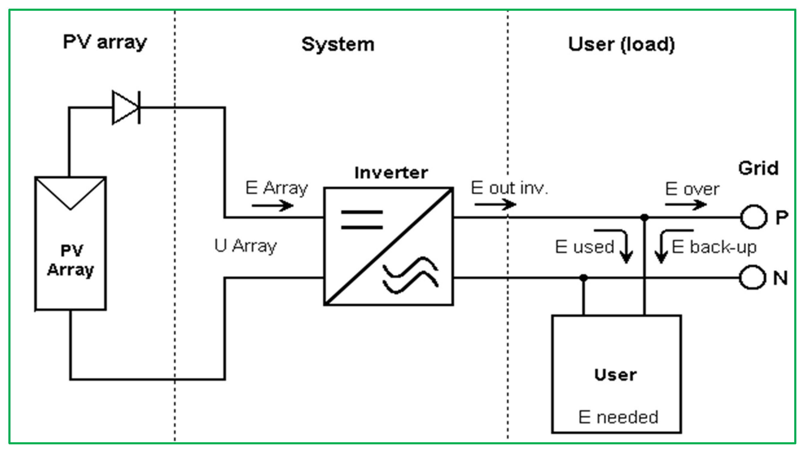
3.1. Proposed System Architecture

Solar irradiation is incident on the PV array, where sunlight is converted into electricity. The PV array output is connected to a DC–DC boost converter input. The inverter’s input is connected to the output of the boost converter. In the inverter, DC voltage is converted into AC voltage. Power from the inverter’s output is injected into the grid and also supplied to fulfill the auxiliary load demand. Figure 10 shows the schematic diagram of the proposed system where the architecture is illustrated into three sections, i.e., PV array, system, and user (load)/grid.

3.2. System Configuration

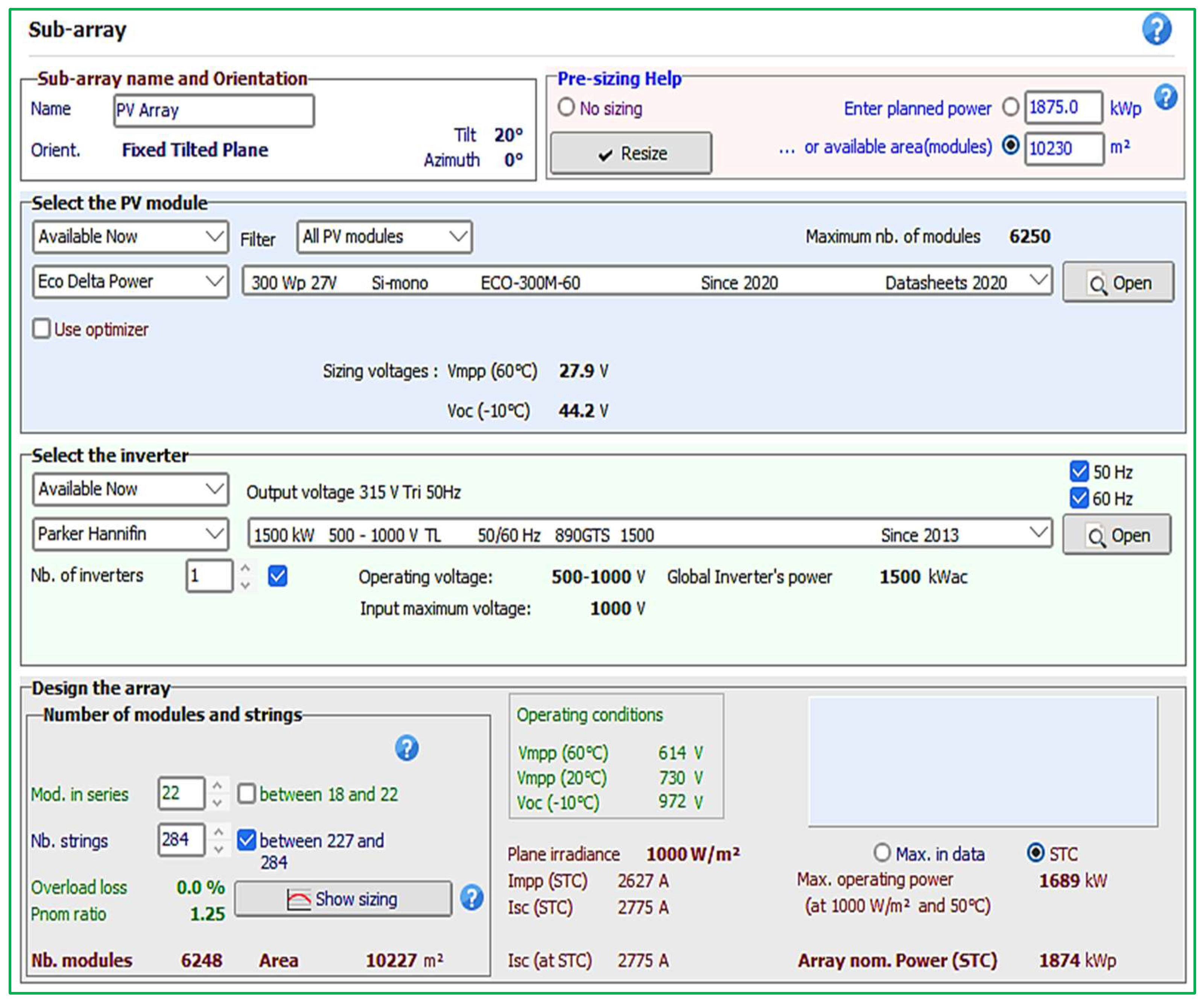
The proposed plant is a grid-connected system in which no 3D scene is defined and no shadings are considered. The system power is 1874 kWp. The system’s power is 1874 kWp means the nominal power in STC is 1874 kWp, during the running of the system there are losses, and after the losses, the actual power remains 1500 kWp, that is, 1.5 MW.

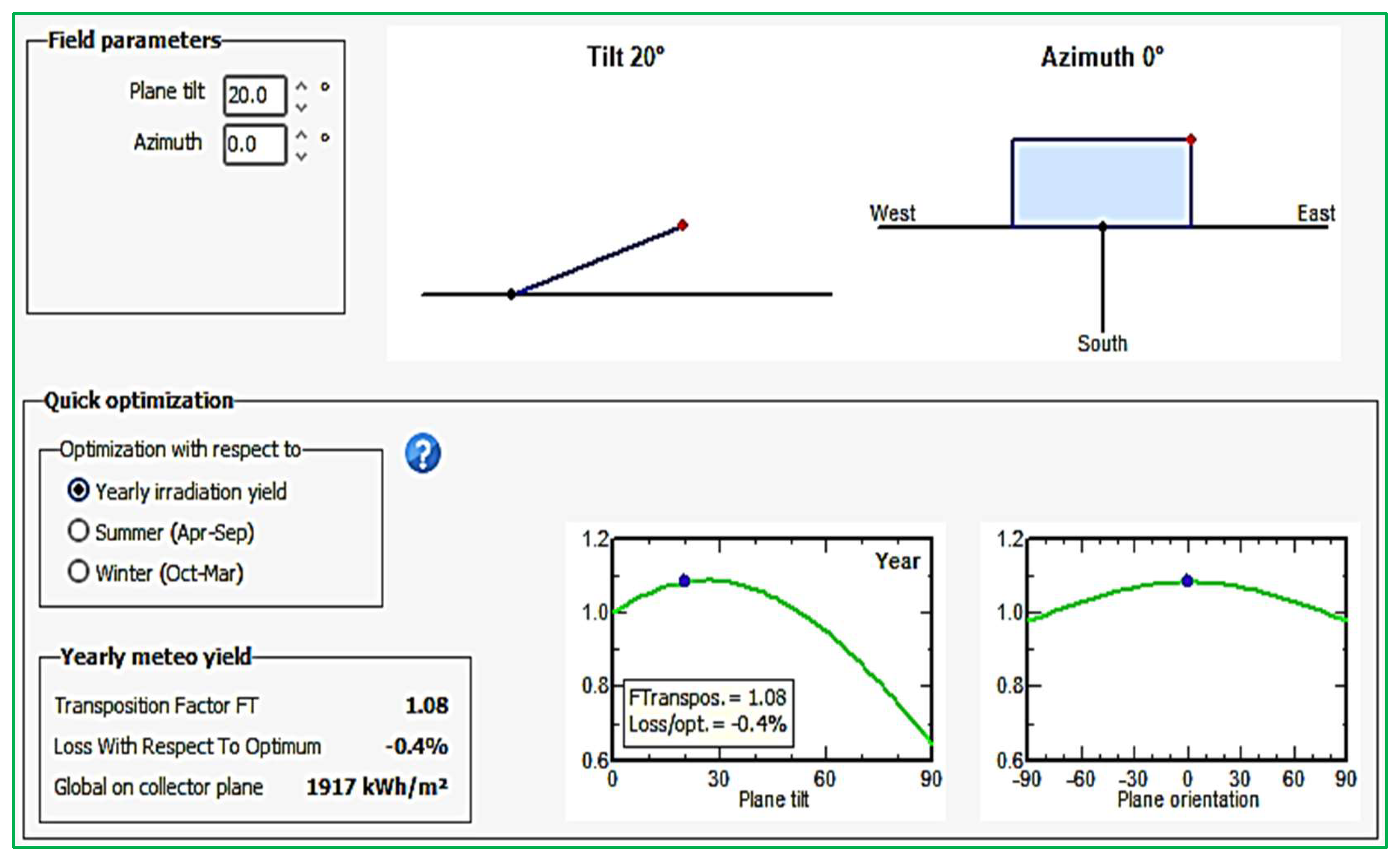
3.2.1. PV Field Orientation

The field type of the PV module and array is a fixed plane. The plane tilt and azimuth of the field array are 20° and 0°, respectively, as shown in Figure 11, where a visual representation as well as quick optimization of the PV field orientation have been depicted. For near shading, no shadings are considered, and no 3D scene is defined in the PVsyst software for the rooftop of the house. The free horizon is considered for the simulation.

3.2.2. PV Array and Inverter Characteristics

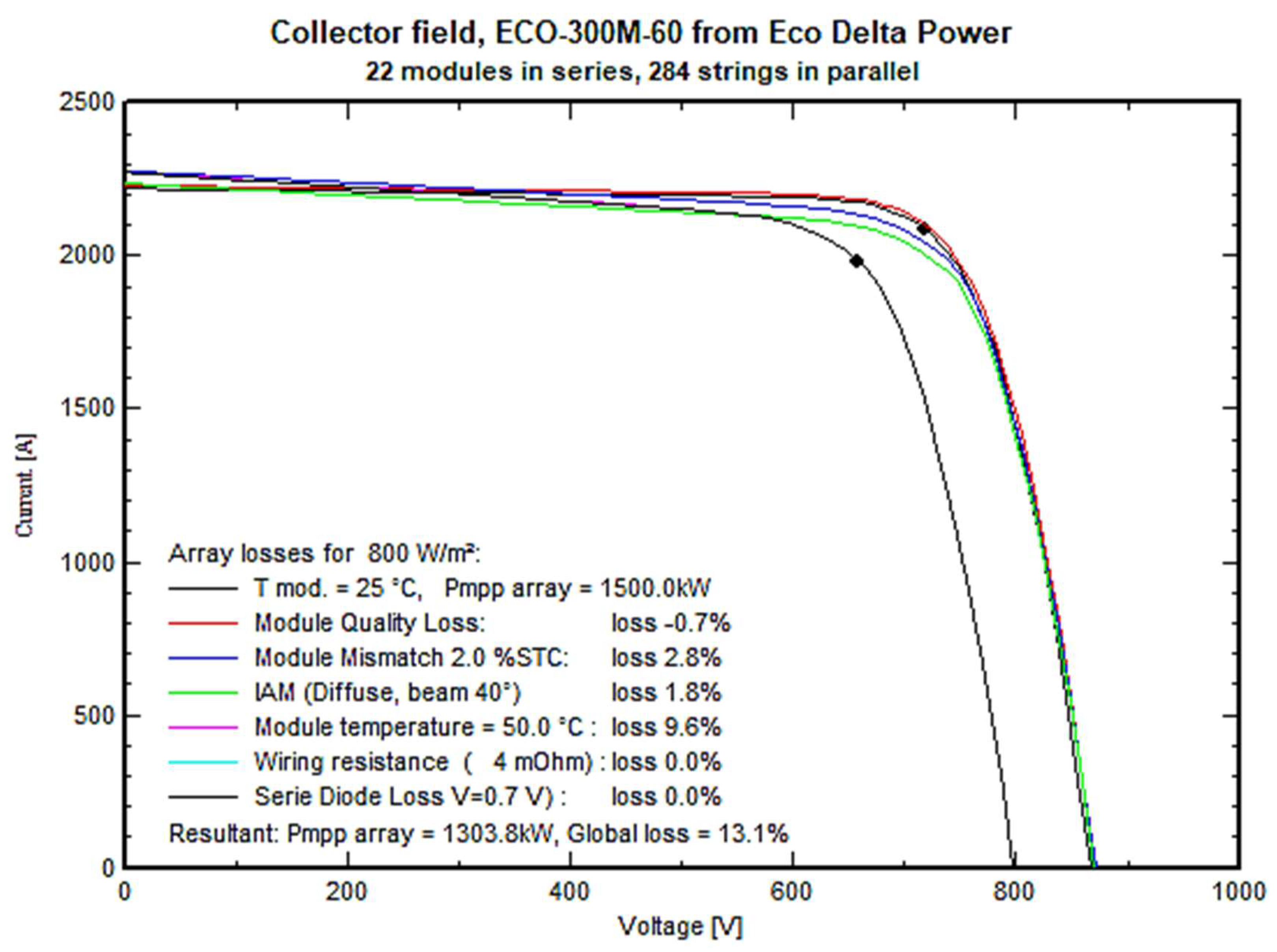
The PV array was made by Eco Delta Power. Its model number, which was taken from the original PVsyst database, is ECO-300M-60. A single unit array has a nominal power (Pnom) of 300 Wp. There are 6248 active PV modules. These 6248 modules are set up in 284 strings, with each string made up of 22 modules connected in series. After installation, there are 10,227 m² of total PV modules and 9110 m² of cells. The nominal power in STC is 1874 kWp. The maximum power points of power (Pmpp), voltage (Vmpp), and current (Impp) for operating conditions at 50 °C are 1689 kWp, 643 V, and 2627 A, respectively. The PV array and inverter characteristics and their details in the design have been shown in Figure 12 which is collected from the PVsyst software.

The manufacturer of the inverter is Parker Hannifin. Its model number is 890GTS_1500 which is collected from the original PVsyst database. The Pnom of the inverter unit is 1500 KWac. The number of used inverters is 1. The operating voltage of the inverter is 500–1000 V. The Pnom ratio is 1.25.

3.3. PV Field and Array Detailed Losses Parameter

Each loss factor of the detailed losses parameters is carefully defined in the software input according to the PV system, as indicated in

Table 2. Detailed losses parameter.

Thermal Loss Factor
Module temperature according to irradiance
Uc (const)	20.0 W/m2K
Uv (wind)	0.0 W/m2K/m/s
Ohmic Losses Series Diode Loss
Voltage drop	0.7 V
Loss fraction	0.1% at STC
DC Wiring Losses
Global array resistance	4.1 mΩ
Loss fraction	1.5% at STC

.

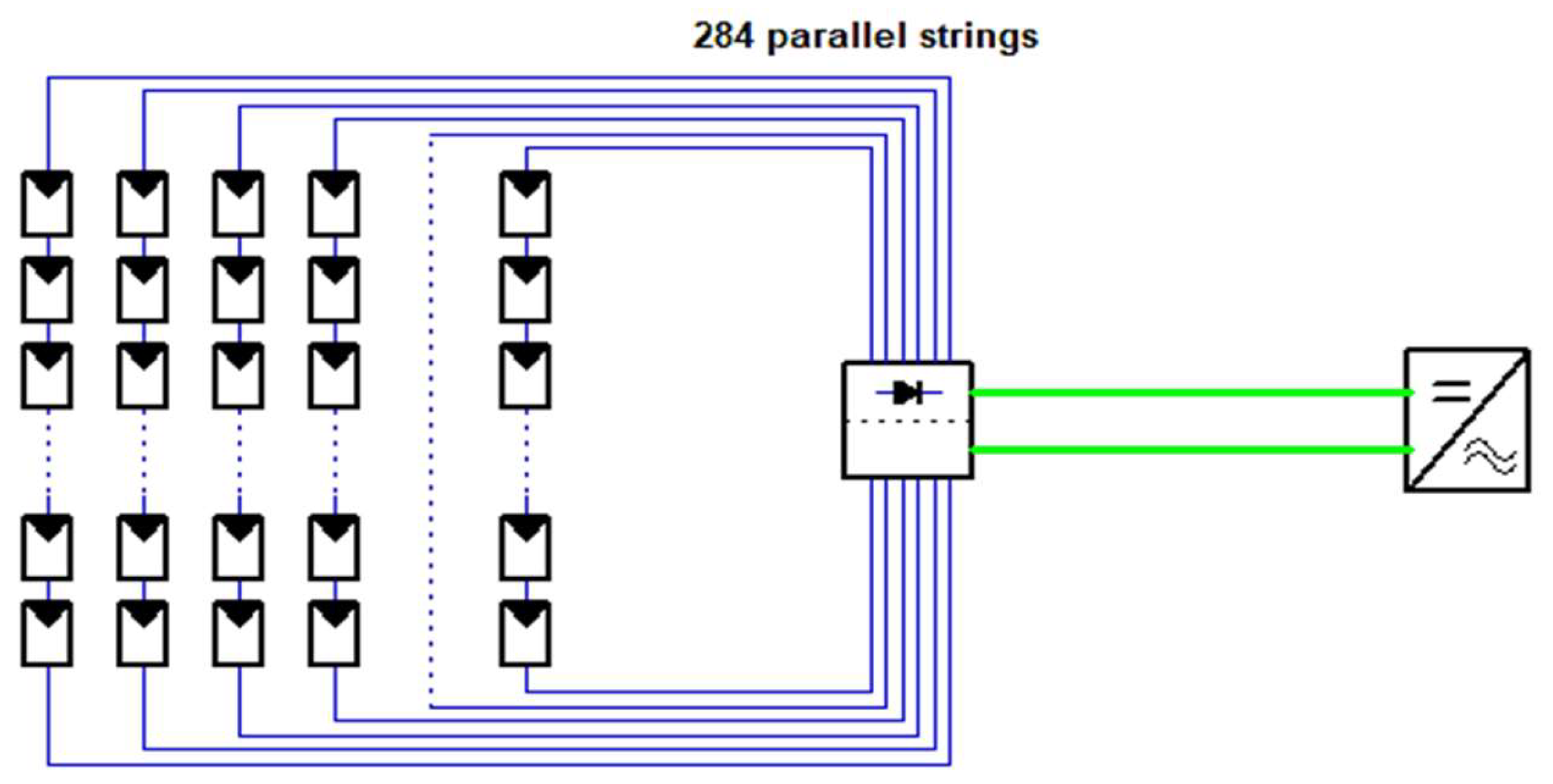
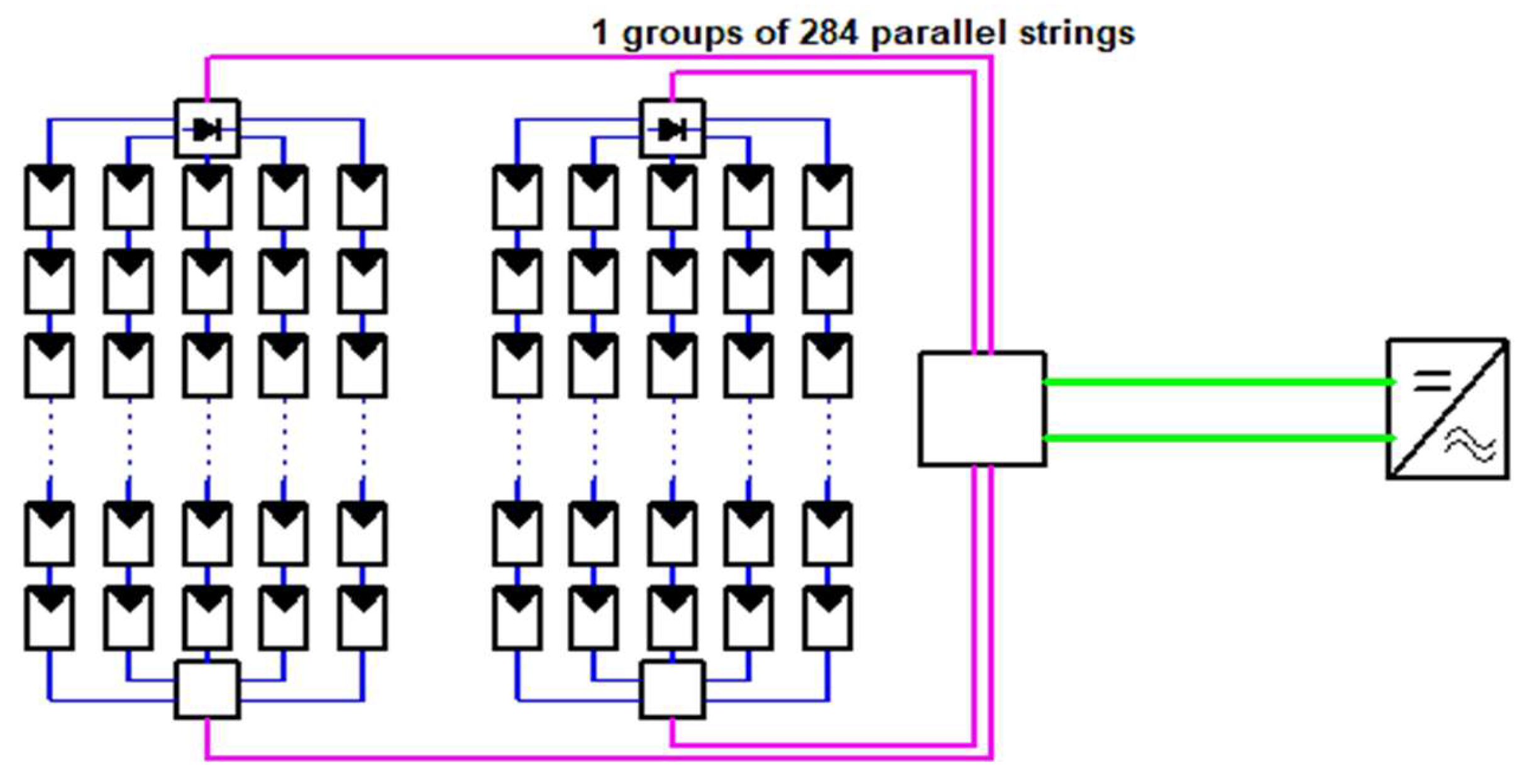
Figure 13 visualizes the wiring layout where 284 strings are created from the total of 6248 modules, each string consisting of 22 modules joined in a series sequence. The wiring diagram for groups of parallel strings, where the input of the inverter is connected to the combined outputs of the parallel strings, is displayed in Figure 14. The loss fraction of different types of losses parameters is defined in percentage for the software input according to the PV system, as indicated in

Table 3. Different types of loss parameter.

Module Quality Loss Loss fraction	−0.8%
LID—Light Induced Degradation Loss fraction	2.0%
Module Mismatch Losses Loss fraction	2.0% at MPP
Strings Mismatch loss Loss fraction	0.1%
Array Soiling Losses Loss fraction	3.0%

.

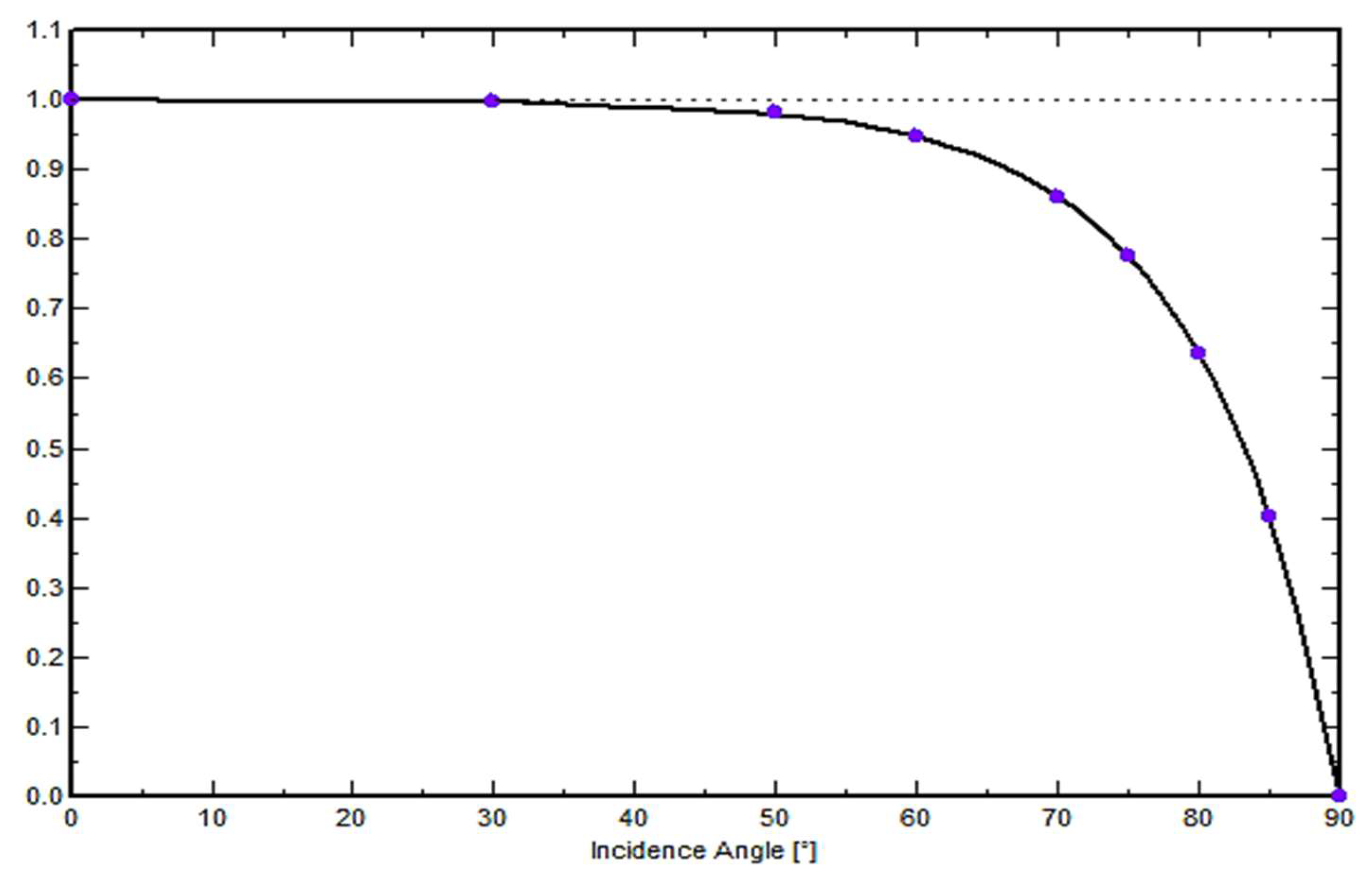
IAM Loss Factor:

The decrease in irradiance that actually reaches the surface of PV cells in comparison to irradiance under normal incidence is known as the incidence effect (abbreviated IAM, for “Incidence Angle Modifier”). Reflections on the glass cover, which increase with the incidence angle, are the primary cause of this drop. The values considered for the IAM are given in the

Table 4. Considered values for IAM.

0°	30°	50°	60°	70°	75°	80°	85°	90°
1.000	0.998	0.981	0.948	0.862	0.776	0.636	0.403	0.000

.

Incidence effect (IAM): Fresnel smooth glass, n = 1.526.

The graphing of the aforementioned information is displayed in Figure 15, also known as the IAM graph. PVsyst’s IAM graph illustrates graphically how the PV modules’ performance changes when the angle of incidence changes. Usually, it displays a curve that illustrates how solar energy decreases as an angle moves away from the optimal perpendicular position.

An illustration of how several factors affect a PV array’s overall performance can be found in PVsyst’s losses graph. Plant designers may improve the design and operation of PV systems to maximize energy production by looking at the losses graph in PVsyst, which provides insights into the intricate relationships of several factors. This graphical representation makes it easier to comprehend in detail how each loss effect affects the PV array’s overall performance. Plotting of the current vs. voltage curves for the loss types under consideration is shown in Figure 16, which displays the PV array behavior for each loss effect in various colors.

3.4. Simulation Modeling

The annualized costs and discount factors from net present costs are calculated using the real discount rate. The variables “Nominal discount rate” and “Expected inflation rate” are used to generate the annual real discount rate, often known as the real interest rate or interest rate.

The following equation is used to obtain the real discount rate:

$$\mathrm{i}=\frac{{\mathrm{i}}^{\prime }-\mathrm{f}}{1+\mathrm{f}}$$

(1)

where i = real discount rate, i′ = nominal discount rate (the rate at which money could be borrowed), and f = expected inflation rate.

The value considered for the nominal discount rate (i′) is 8% and the expected inflation rate (f) is 2%. An annuity, which is a stream of equal yearly cash payments, has a present value that is determined using a ratio called the capital recovery factor. The following equation is used to calculate the capital recovery factor:

$$\mathrm{C}\mathrm{R}\mathrm{F}(\mathrm{i},\mathrm{N})=\frac{\mathrm{i}(1+\mathrm{i}{)}^{\mathrm{N}}}{(1+\mathrm{i}{)}^{\mathrm{N}}-1}$$

(2)

where i = real discount rate, and N = number of years.

The number of years (N) is 25 years, which is the expected lifetime of the PV system.

The present value of all of a system’s lifetime expenses minus the present value of all of its lifetime earnings equals the system’s total net present cost (NPC). Costs include up-front expenses, expenses for repairs and replacements, expenses for operations and maintenance, expenses for fuel, fines for pollution, and the cost of grid electricity. The salvage value as well as grid sales revenue are included in revenues.

The entire annualized cost is used to calculate the levelized cost of energy. The entire annualized cost is equal to the annualized value of the total net present cost. The following equation is used to determine the total annualized cost:

$${\mathrm{C}}_{\mathrm{ann},\mathrm{tot} }=\mathrm{C}\mathrm{R}\mathrm{F}\left(\mathrm{i},\mathrm{N}\right)\cdot {\mathrm{C}}_{\mathrm{N}\mathrm{P}\mathrm{C},\mathrm{tot} }$$

(3)

where C_NPC,tot = the total net present cost [BDT], i = the annual real discount rate [%], N = the project lifetime [year], and CRF (i, N) = a function returning the capital recovery factor.

To calculate the LCOE, the program divides the annual cost of producing electricity (i.e., the total annual cost minus the cost of delivering the thermal load) by the total electric load serviced. The LCOE equation is:

$$\mathrm{L}\mathrm{C}\mathrm{O}\mathrm{E}=\frac{{\mathrm{C}}_{\mathrm{ann},\mathrm{tot}}}{{\mathrm{E}}_{\mathrm{served} }}$$

(4)

where C_ann,tot = total annualized cost of the system [BDT/year], and E_served = total electrical load served [kWh/year].

The following equation is used to determine the total annualized cost when total present cost is considered:

$${\mathrm{C}}_{\mathrm{ann},\mathrm{tot} }=\mathrm{CRF}\left(\mathrm{i},\mathrm{N}\right)\cdot {\mathrm{C}}_{\mathrm{tot} }$$

(5)

where C_tot = the total present cost [BDT], i = the annual real discount rate [%], N = the project lifetime [year], and CRF (i, N) = a function returning the capital recovery factor.

The software divides the annual cost of producing electricity (the total annual cost less the cost of serving the thermal demand) by the total amount of electrical energy produced to arrive at the LCOE. The equation for LCOE is:

$$\mathrm{L}\mathrm{C}\mathrm{O}\mathrm{E}=\frac{{\mathrm{C}}_{\mathrm{ann},\mathrm{tot}}}{{\mathrm{E}}_{\mathrm{g}}}$$

(6)

where C_ann,tot = total annualized cost of the system [BDT/year], and E_g = total electrical energy generated [kWh/year].

4. Results and Discussion

The primary purposes of the PVsyst program are performance analysis and financial assessment of the solar facility. It supports pre-installation modeling by providing essential calculations, including space requirements, energy generation estimations based on allocated space, energy consumption calculations for auxiliary loads from both solar and the grid, injected energy estimations into the grid, and various loss calculations. In terms of financial analysis, the software furnishes data regarding the total installation cost, operational expenses, cost of energy production, payback period, and the potential reduction in CO₂ emissions.

4.1. Performance Analysis

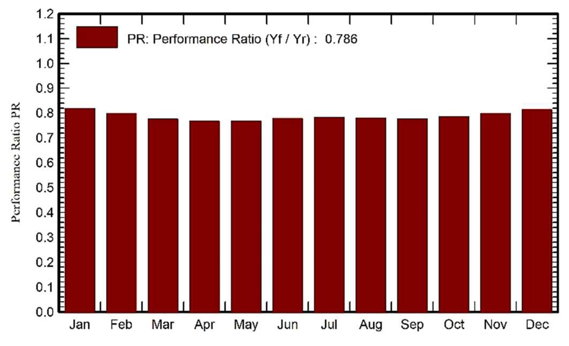
The performance ratio measures how efficiently energy is produced or used in comparison to how much energy would be generated if the system were to run continuously at its nominal STC efficiency. The system’s performance ratio in this instance is 0.786, or 78.63% efficiency as shown in Figure 17.

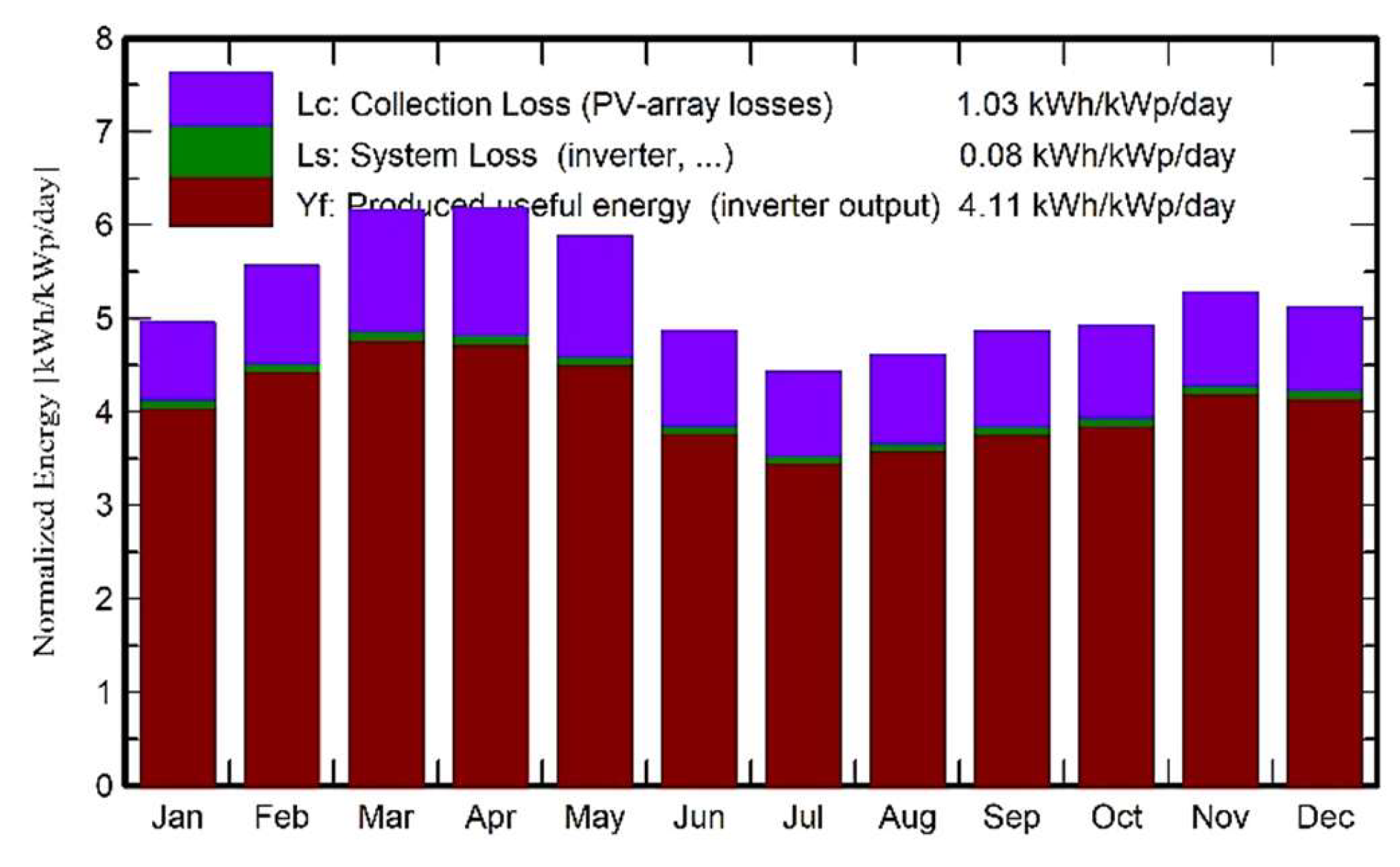
The normalized energy production in Figure 18 draws attention to three key figures: the PV array’s collection loss of 1.03 kWh/kWp/day, the system loss of 0.08 kWh/kWp/day, and the useable energy generated by the inverter output of 4.11 kWh/kWp/day. A solar power plant with a greater normalized energy production will, in contrast to one with a lower normalized energy production, produce more energy per kilowatt of installed capacity. Consequently, a solar power plant demonstrating higher normalized energy production proves to be more productive and cost-effective in its operations.

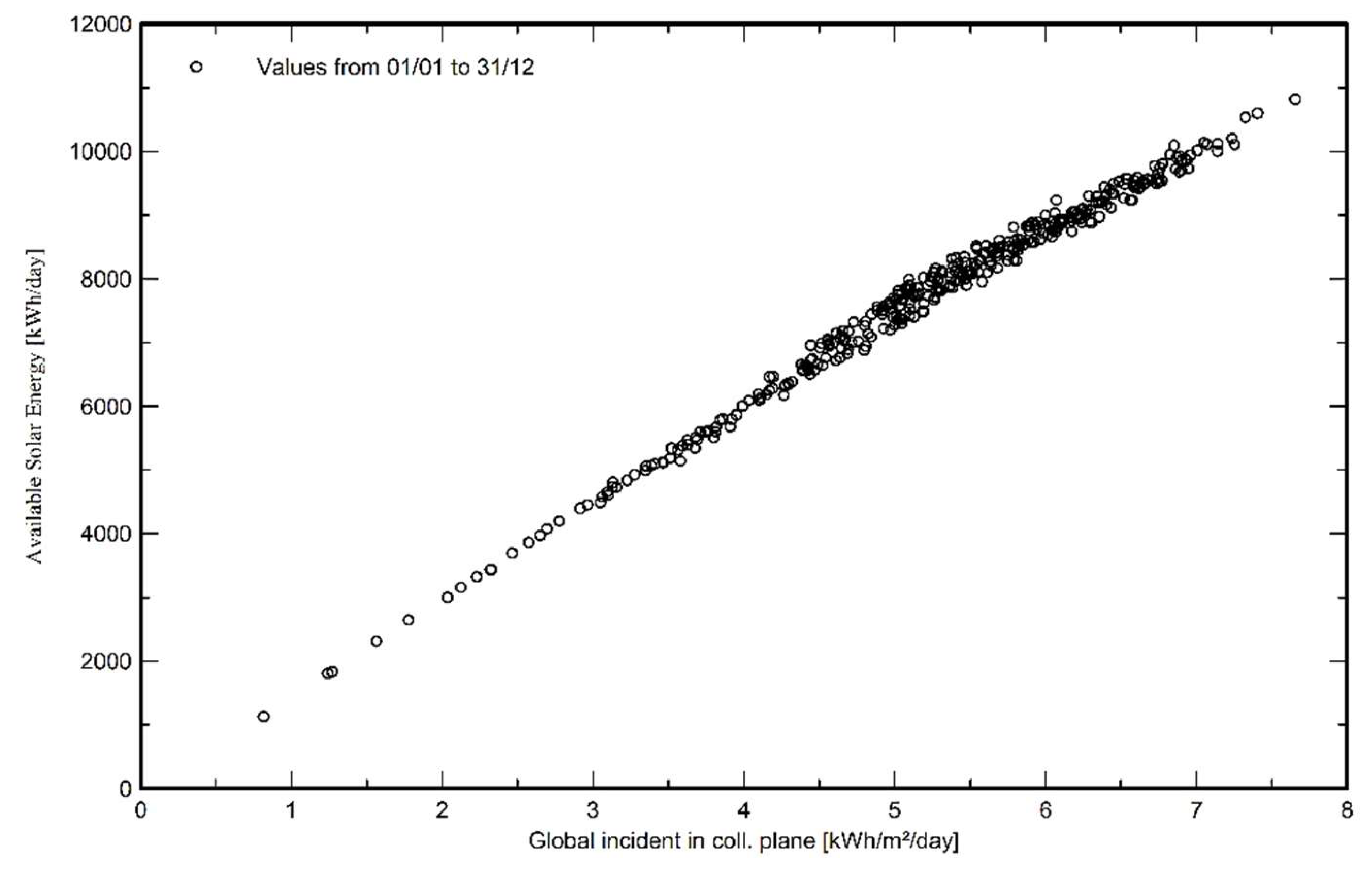
Figure 19 depicts the relationship between the worldwide incident irradiance on the collector plane (measured in kWh/m²/day) and the available solar energy (measured in kWh/day). Daily input/output diagrams are what this illustration is known as. The daily input/output diagram in the PVsyst software is a graphic representation of how the energy generated by a solar power plant varies in response to the daily incident irradiance. This tool is invaluable for comprehending the plant’s performance and pinpointing areas with the potential for enhancement. Ideally, the daily input/output diagram should exhibit a nearly linear trend, albeit with a slight curvature at higher irradiance levels attributed to temperature effects. Any deviation from this pattern, particularly at elevated irradiances, may signify overload conditions on certain days. Monitoring this diagram over time provides insights into the solar power plant’s performance. Changes in the diagram can help to identify issues like reduced energy production or increased losses, enabling timely intervention and system optimization.

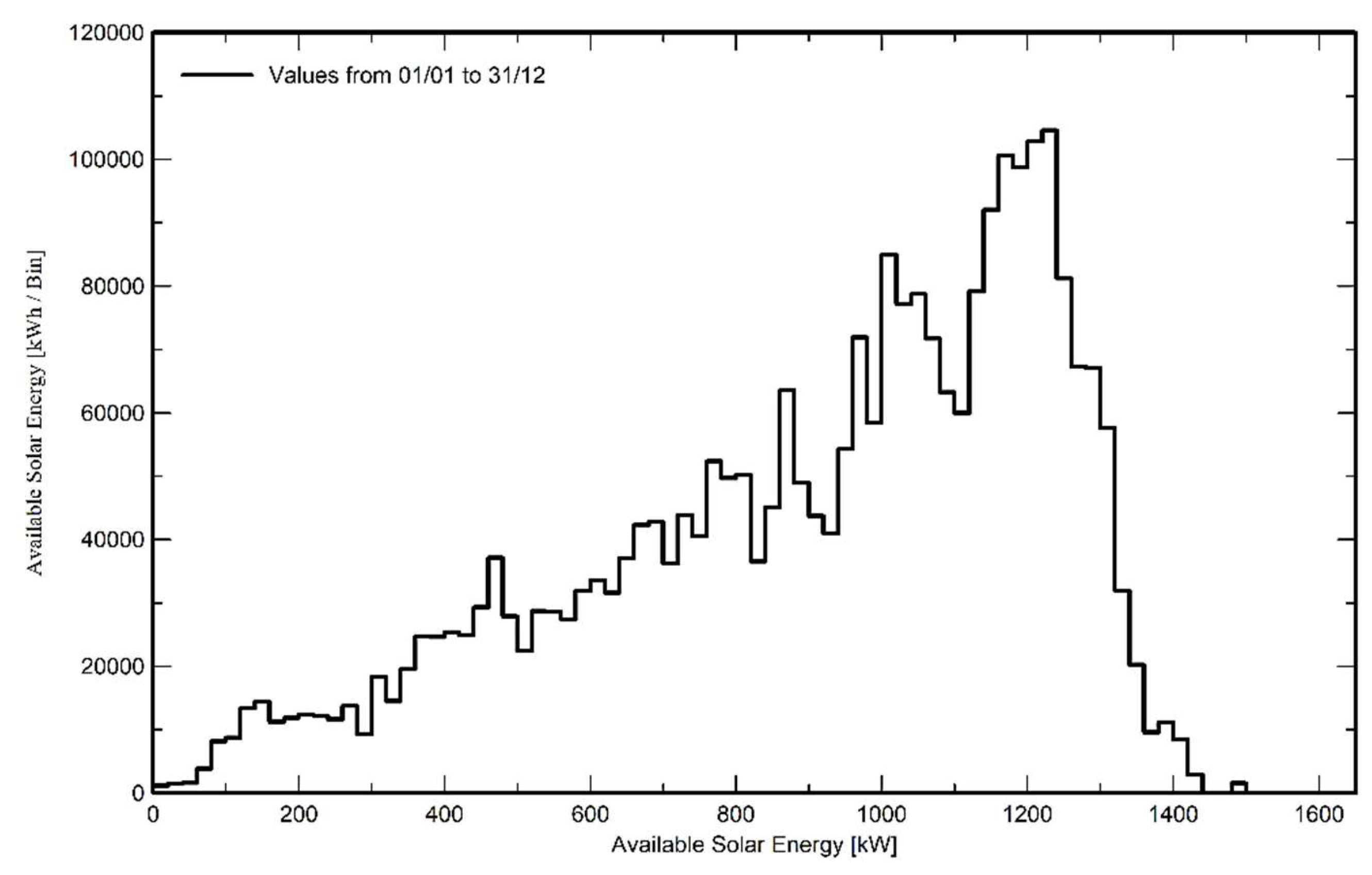
Figure 20, illustrating system output power distribution, presents the relationship between the available solar energy in kW and the available solar energy in kWh per bin (kWh/Bin). In PVsyst software, the system output power distribution graph offers a visual representation of how the power output of a solar power plant is distributed over a specific time span.

Table 5. Balances and main results.

Month	GlobHor kWh/m2	DiffHor kWh/m2	T_Amb °C	GlobInc kWh/m2	GlobEff kWh/m2	EArray MWh	E_User MWh	E_Solar MWh	E_Grid MWh	EFrGrid MWh
January	122.3	54.1	17.35	153.7	145.6	240.7	7.440	3.069	232.8	4.371
February	132.6	60.3	21.49	155.8	147.7	237.9	6.720	3.025	230.2	3.695
March	174.6	78.3	26.48	191.0	180.9	283.4	7.440	3.479	274.4	3.961
April	182.5	88.7	29.10	185.4	175.2	271.9	7.200	3.547	263.1	3.653
May	190.0	100.7	30.27	182.4	171.9	267.5	7.440	3.701	258.6	3.739
June	155.3	99.9	29.46	146.0	137.0	217.5	7.200	3.706	209.3	3.494
July	145.1	99.2	29.24	137.4	128.6	206.0	7.440	3.770	197.9	3.670
August	145.8	90.6	28.99	143.0	134.2	213.7	7.440	3.692	205.5	3.748
September	139.4	74.2	27.91	145.8	137.2	216.8	7.200	3.485	208.8	3.715
October	136.0	72.5	26.95	152.6	144.5	229.4	7.440	3.382	221.3	4.058
November	127.8	54.0	23.13	158.3	150.0	241.5	7.200	2.959	233.9	4.241
December	122.7	50.2	18.73	158.7	150.3	246.6	7.440	3.035	238.7	4.405
Year	1774.2	922.8	25.77	1910.0	1803.1	2872.9	87.600	40.850	2774.4	46.750

Legends: GlobHor—global horizontal irradiation; DiffHor—horizontal diffuse irradiation; T_Amb—ambient temperature; GlobInc—global incident in coll. plane; GlobEff—effective global, corr. for IAM and shadings; EArray—effective energy at the output of the array; E_User—energy supplied to the user; E_Solar—energy from the sun; E_Grid—energy injected into grid; EFrGrid—energy from the grid.

provides detailed balances and main results for every month of a certain year to assess the performance and viability of photovoltaic (PV) systems. These balances and results offer a comprehensive overview of various parameters and outputs related to the solar energy system.

4.2. Loss Diagram

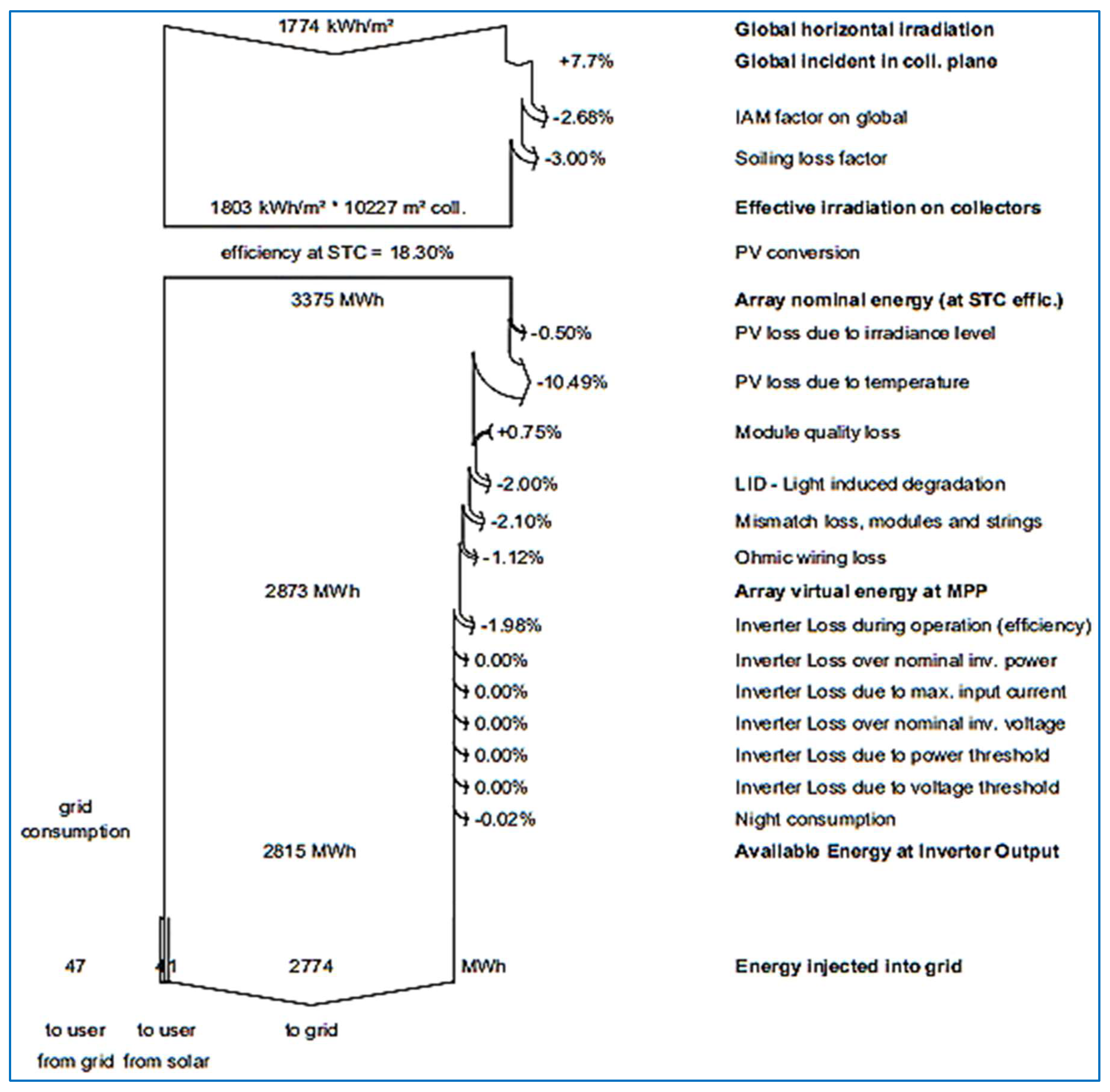
The loss diagram depicted in Figure 21 functions as a visual representation in the form of a system loss flow chart. It serves by breaking down and illustrating the diverse factors contributing to energy losses within a solar installation. Each component, including shading, temperature, module quality, and inverter efficiency, is visually depicted on this diagram, providing users with a clear view of the relative impact of each factor on energy generation [59]. By inputting specific data such as the geographical location, module specifications, and system design, users can generate a tailored loss diagram. This diagram proves to be an invaluable resource for solar professionals and engineers, aiding them in making well-informed decisions to optimize system design and operation. The ultimate goal is to maximize energy production and efficiency while minimizing losses [60]. As such, the loss diagram stands as a critical tool in the design and assessment of the viability of photovoltaic projects.

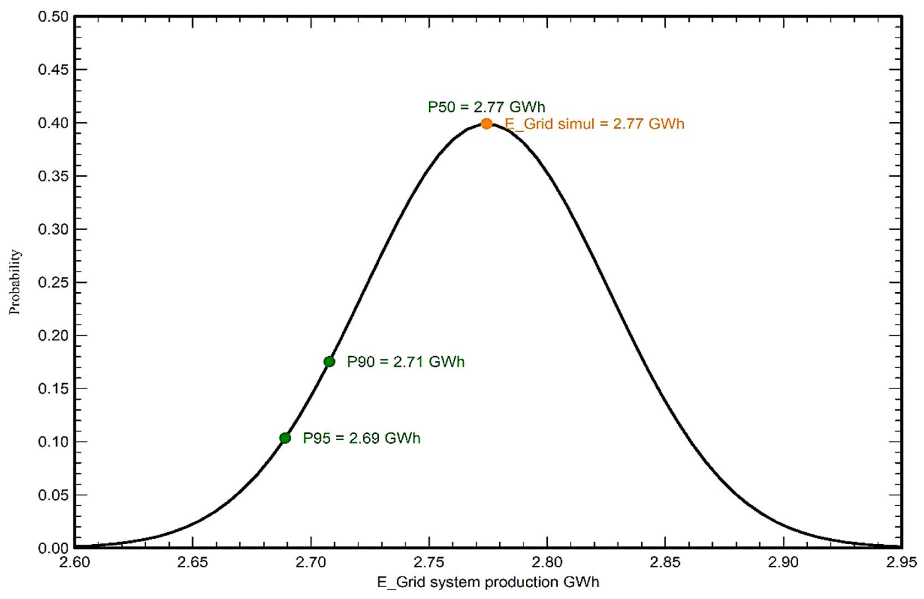
4.3. P50–P90 Evaluation

A probabilistic method for interpreting the simulation results across a number of years is the P50–P90 evaluation as shown in

Table 6. P50–P90 evaluation.

Meteo Data Meteo data source Kind Year-to-year variability (Variance)	Meteonorm 7.3, Sat = 100% Not Defined 0.5%
Specified Deviation Global variability (meteo + system) Variability (Quadratic sum)	1.9%
Simulation and parameters uncertainties PV module modelling/parameters Inverter efficiency uncertainty Soiling and mismatch uncertainties Degradation uncertainty	1.0% 0.5% 1.0% 1.0%
Annual production probability Variability P50 P90 P95	0.05 GWh 2.77 GWh 2.71 GWh 2.69 GWh

. A Gaussian probability distribution is displayed graphically by PVsyst for the number of years. The probability distribution for the plant, where probability is depicted in relation to E_Grid system production in GWh, is displayed in Figure 22.

4.4. Financial Analysis

Financial analysis demonstrates the system’s profitability. Additionally, it displays annual balances in detail between revenues generated by the pricing strategy specified in the tariffs section and costs described in the installation and operating costs section.

Table 7. Installation costs.

Item	Quantity Units	Cost BDT	Total BDT
PV modules ECO-300M-60	6248	12,003.84	75,000,000.00
Inverters 890GTS_1500	1	6,000,000.00	6,000,000.00
Installation settings	1	10,000,000.00	10,000,000.00
Total Depreciable asset			91,000,000.00 91,000,000.00

shows the installation costs, i.e., the costs of PV modules, inverters, and different settings of the system.

Table 8. Operating costs.

Item	Total BDT/Year
Maintenance Cleaning	50,000.00
Total (OPEX) Including inflation (2.00%)	50,000.00 64,060.60

shows the maintenance cost, i.e., the cleaning cost of the solar modules and the maintenance costs of other components of the system. The total installation cost amounts to 91,000,000 BDT, encompassing the initial expenses associated with setting up the solar power plant. This includes costs for solar panels, inverters, mounting systems, and other relevant components. The annual operating cost, considering a 2.00% inflation rate, is 64,060.60 BDT/year. The operating and maintenance cost over 25 years is 1,601,500 BDT. The overall cost over 25 years, inclusive of operation and maintenance, stands at 92,601,500 BDT. This incorporates the total installation cost and the estimated expenses of operating and maintaining the solar power plant over 25 years. This encompasses labor, materials, and other operational costs, with the inflation rate factored in to accommodate the expected rise in goods and services expenses. The energy consumed by auxiliary loads amounts to 87.6 MWh/year (46.4 MWh/year from the grid and 41.2 MWh/year from solar power), representing the energy utilized by auxiliary components within the solar power plant, such as the inverter and monitoring system. Annually, 2774 MWh of energy is supplied to the grid, symbolizing the quantity of energy the solar power plant generates and feeds into the grid. The LCOE stands at 2.82 BDT/kWh, signifying the average cost of generating electricity from the solar power plant throughout its operational life.

Mathematical calculation of LCOE:

Here, ${\mathrm{i}}^{\prime }=$ 8% = 0.08, $\mathrm{f}=$ 2% = 0.02.

Using Equation (1),

$$\begin{gathered} \mathrm{i}=\frac{{\mathrm{i}}^{\prime }-\mathrm{f}}{1+\mathrm{f}} \\ \Rightarrow \mathrm{i}=\frac{0.08-0.02}{1+0.02} \\ \Rightarrow \mathrm{i}=0.0588 \end{gathered}$$

Now, $\mathrm{i}=$ 0.0588, $\mathrm{N}=$ 25 years.

Using Equation (2),

$$\begin{gathered} \mathrm{C}\mathrm{R}\mathrm{F}(\mathrm{i},\mathrm{N})=\frac{\mathrm{i}(1+\mathrm{i}{)}^{\mathrm{N}}}{(1+\mathrm{i}{)}^{\mathrm{N}}-1} \\ \Rightarrow \mathrm{C}\mathrm{R}\mathrm{F}(\mathrm{i},\mathrm{N})=\frac{0.0588(1+0.0588{)}^{25}}{(1+0.0588{)}^{25}-1} \\ \Rightarrow \mathrm{C}\mathrm{R}\mathrm{F}\left(\mathrm{i},\mathrm{N}\right)=0.0773 \end{gathered}$$

Then,

$$\begin{array}{c}{\mathrm{C}}_{\mathrm{tot} }=75,000,000+6,000,000+10,000,000+1,601,500=92,601,500 \mathrm{B}\mathrm{D}\mathrm{T}\hfill \\ \mathrm{i}=0.0588=5.88\%\hfill \\ \mathrm{N}=25 \mathrm{y}\mathrm{e}\mathrm{a}\mathrm{r}\mathrm{s}\hfill \\ \mathrm{CRF}(\mathrm{i}, \mathrm{N})=0.0773\hfill \end{array}$$

Using Equation (3),

$$\begin{gathered} {\mathrm{C}}_{\mathrm{ann},\mathrm{tot} }=\mathrm{C}\mathrm{R}\mathrm{F}\left(\mathrm{i},\mathrm{N}\right)\cdot {\mathrm{C}}_{\mathrm{tot} } \\ \Rightarrow {\mathrm{C}}_{\mathrm{ann},\mathrm{tot} }=0.0773\times 92,601,500 \\ \Rightarrow {\mathrm{C}}_{\mathrm{ann},\mathrm{tot} }=\mathrm{7,158,095.95} \mathrm{B}\mathrm{D}\mathrm{T} \end{gathered}$$

Here,

$$\begin{array}{c}{\mathrm{C}}_{\mathrm{ann},\mathrm{tot} }=\mathrm{7,158,095.95} \mathrm{B}\mathrm{D}\mathrm{T}\hfill \\ {\mathrm{E}}_{\mathrm{g}}=[(2774\times 20)+\{(2774÷2)\times 5\}+(41.2\times 25)]÷25=2537.8 \mathrm{M}\mathrm{W}\mathrm{h}=2,537,800 \mathrm{k}\mathrm{W}\mathrm{h}\hfill \end{array}$$

Using Equation (4),

$$\begin{gathered} \mathrm{L}\mathrm{C}\mathrm{O}\mathrm{E}=\frac{{\mathrm{C}}_{\mathrm{ann},\mathrm{tot} }}{{\mathrm{E}}_{\mathrm{g} }} \\ \Rightarrow \mathrm{L}\mathrm{C}\mathrm{O}\mathrm{E}=\frac{\mathrm{7,158,095.95}}{2,537,800} \\ \Rightarrow \mathrm{L}\mathrm{C}\mathrm{O}\mathrm{E}=2.82 \mathrm{B}\mathrm{D}\mathrm{T} \end{gathered}$$

which is similar to the PVsyst software simulated LCOE = 2.82 BDT/kWh.

The plant’s net present value (NPV), or NPC, is calculated at 232,876,645 BDT by PVsyst software. NPV represents the present value of all future cash flows related to the solar power plant, obtained by discounting future cash flows using an appropriate discount rate. Additionally, the ROI stands at a significant 671.7%, showcasing the return on investment as a percentage. It is derived by dividing the solar power plant’s net present value by the total project cost.

Detailed economic results for every year of the expected project lifetime have been calculated and demonstrated in

Table 9. Detailed economic results (kBDT).

Year	Gross Income	Running Costs	Depreciable Allowance	Taxable Income	Taxes	After-Tax Profit	Self- Consumption Saving	Cumulative Profit	% Amorti.
2024	27,744	50	0	27,694	0	27,694	408	−62,898	30.9%
2025	27,744	51	0	27,693	0	27,693	408	−34,796	61.8%
2026	27,744	52	0	27,692	0	27,692	408	−6696	92.6%
2027	27,744	53	0	27,691	0	27,691	408	21,403	123.5%
2028	27,744	54	0	27,690	0	27,690	408	49,501	154.4%
2029	27,744	55	0	27,689	0	27,689	408	77,598	185.3%
2030	27,744	56	0	27,687	0	27,687	408	105,694	216.1%
2031	27,744	57	0	27,686	0	27,686	408	133,789	247.0%
2032	27,744	59	0	27,685	0	27,685	408	161,883	277.9%
2033	27,744	60	0	27,684	0	27,684	408	189,975	308.8%
2034	27,744	61	0	27,683	0	27,683	408	218,067	339.6%
2035	27,744	62	0	27,682	0	27,682	408	246,157	370.5%
2036	27,744	63	0	27,680	0	27,680	408	274,246	401.4%
2037	27,744	65	0	27,679	0	27,679	408	302,333	432.2%
2038	27,744	66	0	27,678	0	27,678	408	330,420	463.1%
2039	27,744	67	0	27,677	0	27,677	408	358,505	494.0%
2040	27,744	69	0	27,675	0	27,675	408	386,588	524.8%
2041	27,744	70	0	27,674	0	27,674	408	414,671	555.7%
2042	27,744	71	0	27,672	0	27,672	408	442,752	586.5%
2043	27,744	73	0	27,671	0	27,671	408	470,831	617.4%
2044	27,744	74	0	27,670	0	27,670	408	498,909	648.3%
2045	27,744	76	0	27,668	0	27,668	408	526,986	679.1%
2046	27,744	77	0	27,667	0	27,667	408	555,061	710.0%
2047	27,744	79	0	27,665	0	27,665	408	583,134	740.8%
2048	27,744	80	0	27,663	0	27,663	408	611,206	771.7%
Total	693,595	1602	0	691,994	0	691,994	10,212	611,206	771.7%

.

This calculation is based on the energy sold to the grid, which amounts to 2774 MWh/year, and the selling price of energy to the grid, set at 10 BDT/kWh. The gross income is a crucial component of the solar power plant’s cashflow, showcasing the revenue it generates. The operating cost of a 1.5 MW solar power plant over the course of one year is 64,060.60 BDT, while the gross income is 27,744 kBDT, i.e., 27,744,000 BDT. Table 9 and Figure 23 present a comprehensive cashflow analysis of the solar power plant. This cashflow analysis encapsulates all revenues and expenses associated with the solar power plant throughout its operational lifespan. It provides a detailed overview of the financial dynamics, incorporating the gross income generated from selling electricity to the grid. The representation of gross income as a positive cash flow emphasizes its role as a revenue stream for the solar power plant.

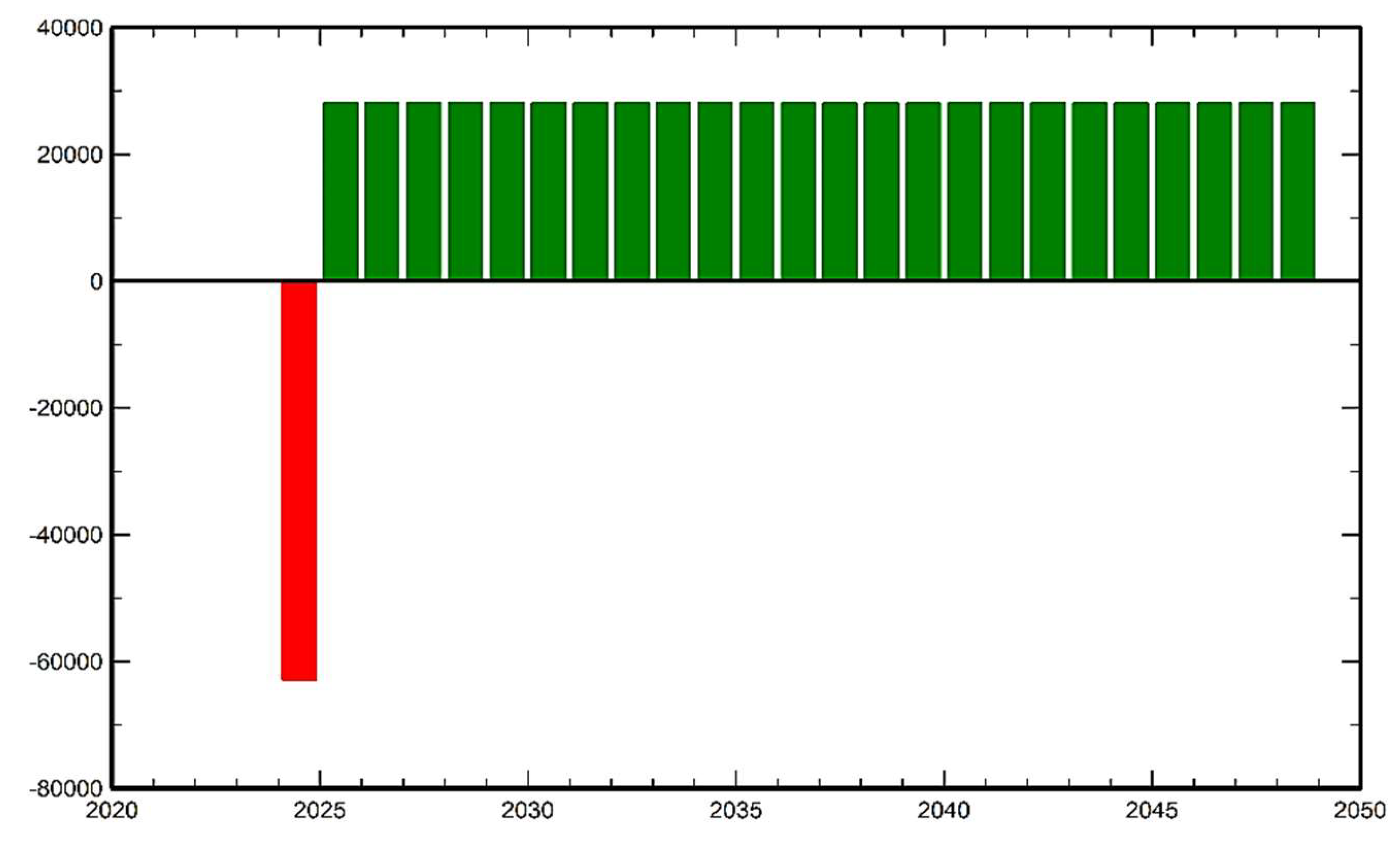
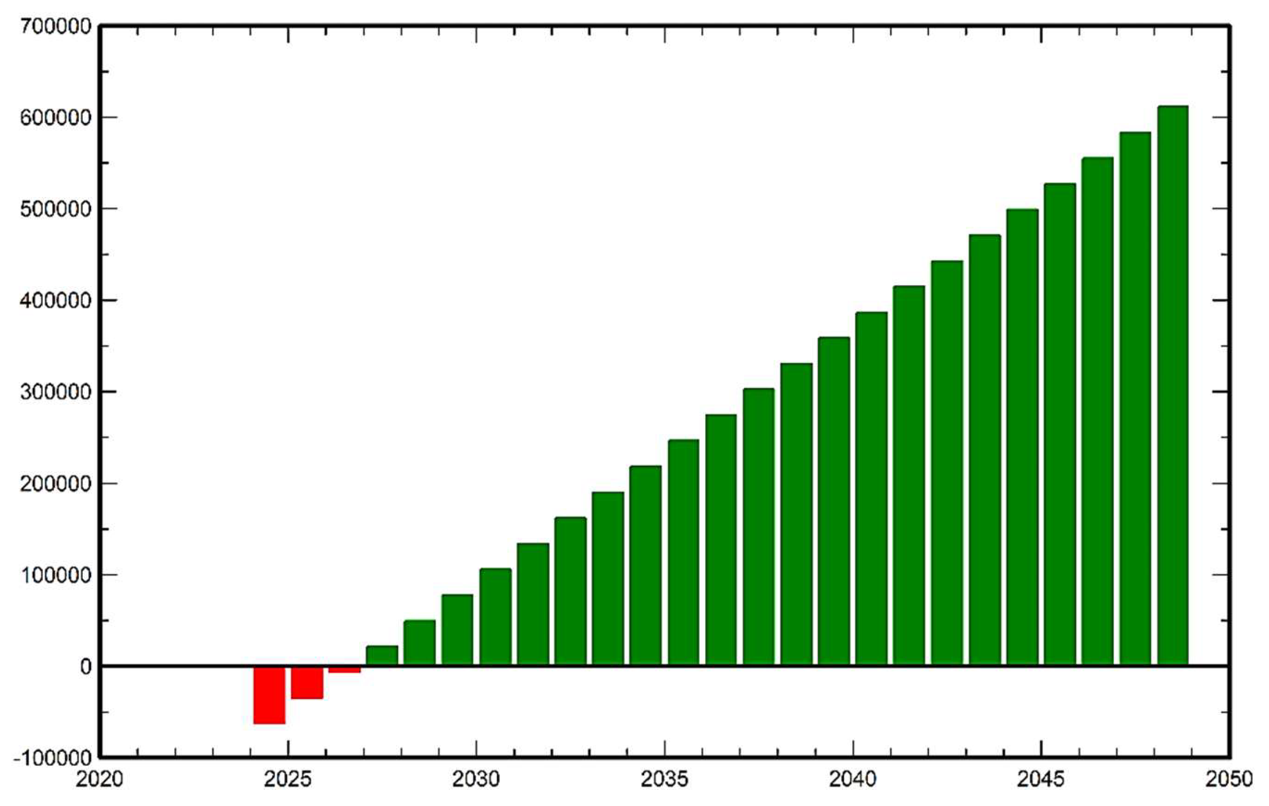
Figure 24 visually presents the cumulative cashflow of the solar power plant. This cumulative cash flow is derived by aggregating the annual cash flows throughout the predefined 25-year project lifespan. By summing up the annual cash flows, we obtain a clear depiction of how the solar power plant’s overall financial performance is anticipated to evolve over the years. The cumulative cash flow serves as a critical metric for assessing the solar power plant’s financial trajectory across its entire operational duration. It provides valuable insights into the financial dynamics and the cumulative impact of revenue generation and expenditure over time. The calculation of the cumulative cash flow is conducted using the specified equation, allowing for a comprehensive evaluation of the solar power plant’s financial sustainability and profitability throughout its projected operational period.

Cumulative cashflow = SUM (Annual cashflow)

where annual cash flow is the cash flow associated with the solar power plant in each year of its lifetime. Figure 24 shows that the cumulative cashflow of the solar power plant is expected to be positive over its lifetime. This means that the solar power plant is expected to generate more revenue than it incurs in expenses. The cumulative cash flow graph is a useful tool for evaluating the financial performance of the solar power plant over its lifetime.

Table 10. Analysis of return on investment (ROI) based on a fixed feed-in tariff.

Electricity Sale Fixed Feed-in Tariff (BDT/kWh)	Net Present Value (NPV) (BDT)	Payback Period (Years)	Return on Investment (ROI) (%)
5.00	72,950,859	6.4	290.6
10.00	232,876,645	3.2	671.7
15.00	392,802,431	2.2	1052.8

demonstrates the analysis of the NPV, payback period, and ROI based on inputting three different fixed feed-in tariff rates to the PVsyst software.

4.5. Calculation of Payback Period

The payback period is the number of years needed to recover the net investment cost as stated in the installation and operational costs section. This period refers to the time it takes for users to recoup their investment through increased efficiency and accurate solar project assessments.

Installation costs = PV modules’ cost + Inverters’ cost + Settings’ cost

= 75,000,000 + 6,000,000 + 10,000,000

= 91,000,000 BDT

Operation and maintenance costs = 64,060.60 BDT/year

Operation and maintenance cost over 25 years = 1,601,500 BDT

Total costs = Installation costs + Operation and maintenance costs over 25 years

= 91,000,000 + 1,601,500

= 92,601,500 BDT

Energy sold to grid = 2774 MWh

Energy consumed by auxiliary load = 41.2 MWh

Total energy generated = 2774 + 41.2 = 2815.2 MWh = 2,815,200 kWh

Total income = 2,815,200 × 10 = 28,152,000 BDT

$$\mathrm{Payback} \mathrm{period}=\frac{Total costs}{Total income}=\frac{\mathrm{92,601,500}}{\mathrm{28,152,000}}=3.2 years$$

After considering all installation and operational costs, and total income, the payback period is 3.2 years. PVsyst aids in minimizing payback periods by optimizing solar installations and maximizing energy production.

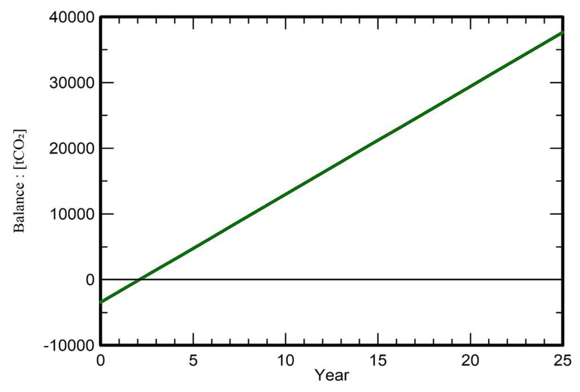
4.6. Carbon Balance

The carbon balancing tool is essential in streamlining the computation of the expected decrease in CO₂ emissions brought on by the installation of a PV system. The life cycle emissions (LCE) concept, which includes all carbon dioxide emissions connected to a particular amount or kind of energy, is the foundation of this computation. These emissions are assessed throughout the component’s complete life cycle, including manufacturing, utilization, maintenance, and disposal, providing a comprehensive view [61].

By utilizing the carbon balance tool, we can determine that the PV system will effectively displace an equivalent amount of current grid power with electricity generated internally. This tool’s justification is that carbon dioxide emissions will be reduced overall if the carbon footprint of the PV system per kWh is lower than that of obtaining energy from the grid [62]. This presents a meaningful way to estimate and promote the positive environmental impact of transitioning to solar energy. The saved CO₂ emission in tCO₂ is plotted against the project lifetime in years in Figure 25.

Therefore, the difference between generated and saved CO₂ emissions is the total carbon balance for a PV plant.

Table 11. System lifecycle emissions details.

Item	LCE	Quantity	Subtotal (kgCO2)
Modules	1713 kgCO2/kWp	1874 kWp	3,210,322
Supports	3.90 kgCO2/kg	62,480 kg	243,377
Inverters	3.90 kgCO2/units	1.00 unit	386
		Total	3454.085

shows the lifecycle emissions details for all the items of the system; it is given in kgCO₂ or tCO₂ and represents the total amount of CO₂ emissions caused by the construction and operation of the components of PV installation.

The LCE grid is expressed in gCO₂/kWh and indicates the average CO₂ emissions per energy unit for grid-produced electricity.

The LCE system is expressed in tCO₂ and represents the total CO₂ emissions brought on by the structure’s construction and operation of the PV installation.

Total energy generated = Energy sold to grid + Energy consumed by auxiliary load

= 2774 + 41.2

= 2815.2 MWh

= 2,815,200 kWh

Project lifetime = 25 years

LCE Grid = 584 gCO₂

LCE System = 3454.1 tCO₂ = 3,454,100,000 gCO₂

Now,

The carbon balance = (Total energy generated × Project lifetime × LCE Grid) − LCE System)

= (2,815,200 kWh × 25 years × 584 gCO₂) − 3,454,100,000 gCO₂

= 41,101,920,000 gCO₂ − 3,454,100,000 gCO₂

= 37,647,820,000 gCO₂ [as 1 tone = 1,000,000 g]

= 37,647.82 tCO₂

Table 12. Comparison of different completed and running solar park projects and this proposed Char Jazira solar power plant in Bangladesh [63,64].

SL.	Project Name	Capacity (MWp)	Location	Latitude, Longitude	Agency	Expected Energy Generation and CO2 Emission Reduction During System Life	Expected Energy Generation and CO2 Emission Reduction until the Data Collection Day
1	200 MW (AC) Solar Park by Beximco Power Co. Ltd.	200	Sundarganj, Gaibandha	25.328795° N, 89.541671° E	BPDB	4 TWh, 2 M tCO2	156 GWh, 74 k tCO2
2	30MW (AC) Solar Park by Intraco CNG Ltd. & Juli New Energy Co. Ltd.	30	Gangachara, Rangpur	25.855312° N, 89.222482° E	BPDB	654 GWh, 309 k tCO2	36 GWh, 17 k tCO2
3	100 MW (AC) Solar Park by Energon Technologies FZE & China Sunergy Co.Ltd (ESUN)	100	Mongla, Bagerhat	22.650135° N, 89.761117° E	BPDB	2 TWh, 1 M tCO2	199 GWh, 94 k tCO2
4	Sirajganj 6.13 MW (AC) Grid-connected Solar Photovoltaic Power Plant	7.6	Sirajganj, Sirajgonj	24.386177° N, 89.748409° E	NWPGCL	166 GWh, 78 k tCO2	22 GWh, 10 k tCO2
5	35 MW AC Solar Park by Consortium of Spectra Engineers Limited & Shunfeng Investment Limited	35	Shibalaya, Manikganj	23.848491° N, 89.913733° E	BPDB	763 GWh, 361 k tCO2	102 GWh, 48 k tCO2
6	50 MW (AC) Solar Park by HETAT-DITROLIC-IFDC Solar Consortium	50	Gauripur, Mymensingh	24.75894° N, 90.59746° E	BPDB	1 TWh, 516 k tCO2	166 GWh, 79 k tCO2
7	Kaptai 7.4 MWp (6.63 MW AC) Grid-connected Solar PV Power Plant	7.4	Kaptai, Rangamati	22.493286° N, 92.218809° E	BPDB	161 GWh, 76 k tCO2	37 GWh, 17 k tCO2
8	8 MW Solar Park by Parasol Energy Ltd.	8	Panchagarh, Panchagarh	26.376098° N, 88.591665° E	BPDB	174 GWh, 82 k tCO2	40 GWh, 19 k tCO2
9	20MW (AC) Solar Park by Joules Power Limited (JPL)	20	Teknaf, Cox’s Bazar	20.980463° N, 92.252503° E	BPDB	436 GWh, 206 k tCO2	116 GWh, 55 k tCO2
10	1.5 MW Grid-connected Solar Power Plant in Lalpur, Natore [Proposed]	1.874	Char Jazira, Lalpur, Natore	24.0900° N, 88.5800° E	Proposed	70.375 GWh, 33074.061 tCO2	Proposed

shows a comparison between the proposed Char Jazira solar power plant and various completed and operational solar park projects in Bangladesh. Location, generation capacity and status of some notable solar farms and future solar initiatives in Bangladesh have been mentioned in

Table 13. Noteworthy solar farms and upcoming solar projects in Bangladesh [1,64].

Location	Generation Capacity (MW)	Project Status
Gangachara, Rangpura	30	Ongoing
Dharmapasha, Sunamganja	32	Ongoing
Gauripur, Mymensingh	50	Ongoing
Chuadangaa	50	Future
Netrokonaa	50	Future
Mongla, Bagerhata	100	Ongoing
Fenia	100	Future
Narsingdia	120	Future
Sundarganj, Gaibandhaa	200	Ongoing

.

5. Conclusions

The escalating consumption of fossil fuels and surging consumer demand have led to frequent occurrences of load shedding. To combat this issue and ensure a continuous supply of electricity, solar energy stands as a promising solution. In this study, we explored the potential of solar energy generation, focusing on addressing the power deficit and reducing reliance on conventional energy sources. The annual solar energy availability of 3375 MWh emphasizes the substantial capacity of solar power. The inverter’s annual output of 2815.2 MWh signifies its ability to generate a significant amount of electricity annually. However, the overall system’s reduced power capacity of 559.8 MWh/year is attributed to diverse losses encountered in the system. Despite this, a notable portion of solar energy, 2774 MWh/year, is successfully integrated into the grid.

An analysis of performance ratios revealed seasonal variations, with the highest PR of 82% in January and the lowest of 77% in April. The yearly average PR of 78.63% indicates the system’s consistent performance and efficiency. Additionally, the solar fraction (SF) of 46.63% underlines the substantial contribution of solar energy in meeting electricity demands. The LCOE at 2.82 BDT per unit demonstrates the economic viability and cost-effectiveness of this solar PV system. A reasonable specific cost per Wp of 48.5 BDT during the investment phase further supports the financial feasibility of the solar project.

Over the plant’s projected 25-year lifespan, the expected energy generation of 70.375 GWh showcases the long-term benefits of solar energy. Remarkably, the calculated payback period of 3 years, 2 months, and 13 days emphasizes the rapid return on investment, highlighting the economic advantages of this sustainable energy solution.

The significant environmental impact is a crucial aspect, with an impressive reduction of 37,647.82 tCO₂ emissions over the 25-year lifespan, reflecting the positive contribution of solar energy in reducing carbon footprints and promoting environmental sustainability. In conclusion, this solar technology proves to be a green and clean energy source, making substantial strides toward a more sustainable and eco-friendly future.

Solar power plants have revolutionized clean energy production but face several shortcomings. One primary limitation is their intermittent nature due to dependency on sunlight. Energy-storage systems like batteries help to mitigate this issue but are expensive and have limited storage capacities. Efficiency remains another challenge; while solar panels have improved, they still cannot convert all sunlight into usable energy.

Future research aims to address these limitations. Improving energy-storage systems is crucial for a consistent power supply. Advancements in battery technology or alternative storage methods such as molten salt, compressed air, or hydrogen are under exploration. Enhancing solar panel efficiency via new materials, designs, and integrated technologies could significantly boost energy output. Innovations in flexible and transparent panels might enable diverse applications. Research on reducing environmental impact involves designing eco-friendly installation methods, recycling solar components, and utilizing less land-intensive solar technologies like floating solar farms or integrating them into infrastructures like highways or buildings.

References

- Solar Energy in Bangladesh: Current Status and Future. Available online: https://energytracker.asia/solar-energy-in-bangladesh-current-status-and-future/?fbclid=IwAR2dpVoe0scUzqZ_VGKQm2M3jkzN0UawrjmlbM3h9i0F_wGdD874jBmZUzg (accessed on 4 September 2023).
- Hossain, M.A.; Pota, H.R.; Hossain, M.J.; Blaabjerg, F. Evolution of Microgrids with Converter-Interfaced Generations: Challenges and Opportunities. Int. J. Electr. Power Energy Syst. 2019, 109, 160–186. [Google Scholar] [CrossRef]
- Karmaker, A.K.; Islam, S.M.R.; Kamruzzaman, M.; Rashid, M.M.U.; Faruque, M.O.; Hossain, M.A. Smart City Transformation: An Analysis of Dhaka and Its Challenges and Opportunities. Smart Cities 2023, 6, 1087–1108. [Google Scholar] [CrossRef]
- Alam, M.S.; Chowdhury, T.A.; Dhar, A.; Al-Ismail, F.S.; Choudhury, M.S.H.; Shafiullah, M.; Hossain, M.I.; Hossain, M.A.; Ullah, A.; Rahman, S.M. Solar and Wind Energy Integrated System Frequency Control: A Critical Review on Recent Developments. Energies 2023, 16, 812. [Google Scholar] [CrossRef]
- Hasan, M.; Tanvir, A.A.; Siddiquee, S.M.S.; Zubair, A. Efficient Hybrid Renewable Energy System for Industrial Sector with On-Grid Time Management. In Proceedings of the 2015 3rd International Conference on Green Energy and Technology (ICGET), Dhaka, Bangladesh, 11 September 2015; pp. 4–9. [Google Scholar] [CrossRef]
- Duman, A.C.; Güler, Ö. Economic Analysis of Grid-Connected Residential Rooftop PV Systems in Turkey. Renew. Energy 2020, 148, 697–711. [Google Scholar] [CrossRef]
- Ihsan, M.A.; Eram, A.F.; Khadem, M.M. Viability Study of Net Metering Scheme in Residential Scale: A Bangladeshi Perspective. In Proceedings of the 2022 International Conference on Computational Intelligence and Sustainable Engineering Solutions (CISES), Greater Noida, India, 20–21 May 2022; pp. 361–365. [Google Scholar] [CrossRef]
- JPI Urban Europe. Positive Energy Districts (PED). Available online: https://jpi-urbaneurope.eu/ped/ (accessed on 9 November 2023).
- Chen, Y.; Wang, J.; Lund, P.D. Sustainability Evaluation and Sensitivity Analysis of District Heating Systems Coupled to Geothermal and Solar Resources. Energy Convers. Manag. 2020, 220, 113084. [Google Scholar] [CrossRef]
- Bottecchia, L.; Gabaldón, A.; Castillo-Calzadilla, T.; Soutullo, S.; Ranjbar, S.; Eicker, U. Fundamentals of Energy Modelling for Positive Energy Districts. In Smart Innovation, Systems and Technologies; Springer: Singapore, 2022; Volume 263, pp. 435–445. [Google Scholar] [CrossRef]
- Lindholm, O.; Rehman, H.U.; Reda, F. Positioning Positive Energy Districts in European Cities. Buildings 2021, 11, 19. [Google Scholar] [CrossRef]
- Moreno, A.G.; Vélez, F.; Alpagut, B.; Hernández, P.; Montalvillo, C.S. How to Achieve Positive Energy Districts for Sustainable Cities: A Proposed Calculation Methodology. Sustainability 2021, 13, 710. [Google Scholar] [CrossRef]
- Alpagut, B.; Akyürek, Ö.; Mitre, E.M. Positive Energy Districts Methodology and Its Replication Potential. Multidiscip. Digit. Publ. Inst. Proc. 2019, 20, 8. [Google Scholar] [CrossRef]
- Bagheri, M.; Shirzadi, N.; Bazdar, E.; Kennedy, C.A. Optimal Planning of Hybrid Renewable Energy Infrastructure for Urban Sustainability: Green Vancouver. Renew. Sustain. Energy Rev. 2018, 95, 254–264. [Google Scholar] [CrossRef]
- Castillo-Calzadilla, T.; Garay-Martinez, R.; Andonegui, C.M. Holistic Fuzzy Logic Methodology to Assess Positive Energy District (PathPED). Sustain. Cities Soc. 2023, 89, 104375. [Google Scholar] [CrossRef]
- Zhang, X.; Penaka, S.R.; Giriraj, S.; Sánchez, M.N.; Civiero, P.; Vandevyvere, H. Characterizing Positive Energy District (PED) through a Preliminary Review of 60 Existing Projects in Europe. Buildings 2021, 11, 318. [Google Scholar] [CrossRef]
- Marotta, I.; Guarino, F.; Longo, S.; Cellura, M. Environmental Sustainability Approaches and Positive Energy Districts: A Literature Review. Sustainability 2021, 13, 13063. [Google Scholar] [CrossRef]
- Krangsås, S.G.; Steemers, K.; Konstantinou, T.; Soutullo, S.; Liu, M.; Giancola, E.; Prebreza, B.; Ashrafian, T.; Murauskaitė, L.; Maas, N. Positive Energy Districts: Identifying Challenges and Interdependencies. Sustainability 2021, 13, 10551. [Google Scholar] [CrossRef]
- Neumann, H.M.; Hainoun, A.; Stollnberger, R.; Etminan, G.; Schaffler, V. Analysis and Evaluation of the Feasibility of Positive Energy Districts in Selected Urban Typologies in Vienna Using a Bottom-Up District Energy Modelling Approach. Energies 2021, 14, 4449. [Google Scholar] [CrossRef]
- Poudyal, R.; Loskot, P.; Parajuli, R. Techno-Economic Feasibility Analysis of a 3-KW PV System Installation in Nepal. Renew. Wind. Water Sol. 2021, 8, 5. [Google Scholar] [CrossRef]
- Imam, A.A.; Al-Turki, Y.A.; Sreerama Kumar, R. Techno-Economic Feasibility Assessment of Grid-Connected PV Systems for Residential Buildings in Saudi Arabia—A Case Study. Sustainability 2020, 12, 262. [Google Scholar] [CrossRef]
- Faiz, F.U.H.; Shakoor, R.; Raheem, A.; Umer, F.; Rasheed, N.; Farhan, M. Modeling and Analysis of 3 MW Solar Photovoltaic Plant Using PVSyst at Islamia University of Bahawalpur, Pakistan. Int. J. Photoenergy 2021, 2021, 6673448. [Google Scholar] [CrossRef]
- Baqir, M.; Channi, H.K. Analysis and Design of Solar PV System Using Pvsyst Software. Mater. Today Proc. 2022, 48, 1332–1338. [Google Scholar] [CrossRef]
- Kumar, R.; Rajoria, C.S.; Sharma, A.; Suhag, S. Design and Simulation of Standalone Solar PV System Using PVsyst Software: A Case Study. Mater. Today Proc. 2020, 46, 5322–5328. [Google Scholar] [CrossRef]
- Satish, M.; Santhosh, S.; Yadav, A. Simulation of a Dubai Based 200 KW Power Plant Using PVsyst Software. In Proceedings of the 2020 7th International Conference on Signal Processing and Integrated Networks (SPIN), Noida, India, 27–28 February 2020; pp. 824–827. [Google Scholar] [CrossRef]
- Jagadale, P.; Choudhari, A.; Jadhav, S. Design and Simulation of Grid Connected Solar Si-Poly Photovoltaic Plant Using PVsyst For Pune, India Location. Renew. Energy Res. Appl. 2022, 3, 41–49. [Google Scholar]
- Grover, A.; Khosla, A.; Joshi, D. Design and Simulation of 20MW Photovoltaic Power Plant Using PVSyst. Indones. J. Electr. Eng. Comput. Sci. 2020, 19, 58–65. [Google Scholar] [CrossRef]
- Chauhan, A.; Sharma, M.; Baghel, S. Designing and Performance Analysis of 15KWP Grid Connection Photovoltaic System Using Pvsyst Software. In Proceedings of the 2020 Second International Conference on Inventive Research in Computing Applications (ICIRCA), Coimbatore, India, 15–17 July 2020; pp. 1003–1008. [Google Scholar] [CrossRef]
- Kapoor, S.; Sharma, A.K.; Porwal, D. Design and Simulation of 60kWp Solar On-Grid System for Rural Area in Uttar-Pradesh by “PVsyst”. J. Phys. Conf. Ser. 2021, 2070, 012147. [Google Scholar] [CrossRef]
- Belmahdi, B.; El Bouardi, A. Solar Potential Assessment Using PVsyst Software in the Northern Zone of Morocco. Procedia Manuf. 2020, 46, 738–745. [Google Scholar] [CrossRef]
- Tamoor, M.; Bhatti, A.R.; Farhan, M.; Miran, S.; Raza, F.; Zaka, M.A. Designing of a Hybrid Photovoltaic Structure for an Energy-Efficient Street Lightning System Using PVsyst Software. Eng. Proc. 2021, 12, 10–14. [Google Scholar] [CrossRef]
- Mohammadi, S.A.D.; Gezegin, C. Design and Simulation of Grid-Connected Solar PV System Using PVSYST, PVGIS and HOMER Software. Int. J. Pioneer. Technol. Eng. 2022, 1, 36–41. [Google Scholar] [CrossRef]
- PVsyst—Logiciel Photovoltaïque. Available online: https://www.pvsyst.com/ (accessed on 1 September 2023).
- Dalal, S.; Jadhav, V.; Raut, R.; Narkhede, S. Analysis of 1kw solar rooftop system by using pvsyst. In Proceedings of the 2nd International Conference on Communication & Information Processing (ICCIP), Tokyo, Japan, 27–29 November 2020; pp. 1–8. [Google Scholar]
- Solar Panel Orientation—Energy Education. Available online: https://energyeducation.ca/encyclopedia/Solar_panel_orientation (accessed on 1 September 2023).
- Tilt and Orientation and Solar Energy. Available online: https://www.viridiansolar.co.uk/resources-1-3-tilt-and-orientation.html (accessed on 1 September 2023).
- Bansal, N.; Pany, P.; Singh, G. Visual Degradation and Performance Evaluation of Utility Scale Solar Photovoltaic Power Plant in Hot and Dry Climate in Western India. Case Stud. Therm. Eng. 2021, 26, 101010. [Google Scholar] [CrossRef]
- Talavera, D.L.; Muñoz-Cerón, E.; de la Casa, J.; Lozano-Arjona, D.; Theristis, M.; Pérez-Higueras, P.J. Complete Procedure for the Economic, Financial and Cost-Competitiveness of Photovoltaic Systems with Self-Consumption. Energies 2019, 12, 345. [Google Scholar] [CrossRef]
- Cui, Y.; Zhu, J.; Meng, F.; Zoras, S.; McKechnie, J.; Chu, J. Energy Assessment and Economic Sensitivity Analysis of a Grid-Connected Photovoltaic System. Renew. Energy 2020, 150, 101–115. [Google Scholar] [CrossRef]
- Meteo Database > Import Meteo Data > Meteonorm Data and Program. Available online: https://www.pvsyst.com/help/meteo_source_meteonorm.htm (accessed on 1 September 2023).
- Intro—Meteonorm (En). Available online: https://meteonorm.meteotest.ch/en/ (accessed on 1 September 2023).
- NASA Technical Reports Server (NTRS). Surface Meteorology and Solar Energy (SSE) Data Release 5.1. Available online: https://ntrs.nasa.gov/citations/20080012141 (accessed on 1 September 2023).
- Solargis. Solar Resource Maps and GIS Data for 200+ Countries. Available online: https://solargis.com/maps-and-gis-data/download/bangladesh (accessed on 1 September 2023).
- Gostein, M.; Hoffmann, A.; Farina, F.; Stueve, B. Measuring Global, Direct, and Diffuse Irradiance Using a Reference Cell Array. In Proceedings of the 2021 IEEE 48th Photovoltaic Specialists Conference (PVSC), Fort Lauderdale, FL, USA, 20–25 June 2021; pp. 923–927. [Google Scholar] [CrossRef]
- PV Performance Modeling Collaborative (PVPMC). Direct Normal Irradiance. Available online: https://pvpmc.sandia.gov/modeling-guide/1-weather-design-inputs/irradiance-insolation/direct-normal-irradiance/ (accessed on 9 November 2023).
- Zhang, C.; Yan, Z.; Ma, C.; Xu, X. Prediction of Direct Normal Irradiation Based on CNN-LSTM Model. In Proceedings of the Proceedings of the 2020 5th International Conference on Multimedia Systems and Signal Processing, Chengdu, China, 28–30 May 2020; pp. 74–80. [Google Scholar] [CrossRef]
- PV Performance Modeling Collaborative (PVPMC). Diffuse Horizontal Irradiance. Available online: https://pvpmc.sandia.gov/modeling-guide/1-weather-design-inputs/irradiance-insolation/diffuse-horizontal-irradiance/ (accessed on 9 November 2023).
- Dubey, S.; Sarvaiya, J.N.; Seshadri, B. Temperature Dependent Photovoltaic (PV) Efficiency and Its Effect on PV Production in the World—A Review. Energy Procedia 2013, 33, 311–321. [Google Scholar] [CrossRef]
- Boston Solar. How Temperature & Shade Affect Solar Panel Efficiency. Available online: https://www.bostonsolar.us/solar-blog-resource-center/blog/how-do-temperature-and-shade-affect-solar-panel-efficiency/ (accessed on 9 November 2023).
- Wind Effect on Solar Panels—AESOLAR. Available online: https://ae-solar.com/wind-effect-on-solar-panels/ (accessed on 9 November 2023).
- Bhattacharya, T.; Chakraborty, A.K.; Pal, K. Effects of Ambient Temperature and Wind Speed on Performance of Monocrystalline Solar Photovoltaic Module in Tripura, India. J. Sol. Energy 2014, 2014, 817078. [Google Scholar] [CrossRef]
- Eltbaakh, Y.A.; Ruslan, M.H.; Alghoul, M.A.; Othman, M.Y.; Sopian, K.; Razykov, T.M. Solar Attenuation by Aerosols: An Overview. Renew. Sustain. Energy Rev. 2012, 16, 4264–4276. [Google Scholar] [CrossRef]
- Page, J.K. Radiation Data. In Solar Energy Conversion II; Elsevier: Amsterdam, The Netherlands, 1981; pp. 23–35. [Google Scholar] [CrossRef]
- ScienceDirect Topics. Linke Turbidity Factor—An Overview. Available online: https://www.sciencedirect.com/topics/engineering/linke-turbidity-factor (accessed on 9 November 2023).
- Shrestha, A.K.; Thapa, A.; Gautam, H. Solar Radiation, Air Temperature, Relative Humidity, and Dew Point Study: Damak, Jhapa, Nepal. Int. J. Photoenergy 2019, 2019, 8369231. [Google Scholar] [CrossRef]
- Sohani, A.; Shahverdian, M.H.; Sayyaadi, H.; Garcia, D.A. Impact of Absolute and Relative Humidity on the Performance of Mono and Poly Crystalline Silicon Photovoltaics; Applying Artificial Neural Network. J. Clean. Prod. 2020, 276, 123016. [Google Scholar] [CrossRef]
- Bowen, A. Fundamentals of solar architecture. In Solar Energy Conversion; Elsevier: Amsterdam, The Netherlands, 1979; pp. 481–553. [Google Scholar] [CrossRef]
- Yousef, B.A.A.; Radwan, A.; Olabi, A.G.; Abdelkareem, M.A. Sun Composition, Solar Angles, and Estimation of Solar Radiation. In Renewable Energy—Volume 1: Solar, Wind, and Hydropower: Definitions, Developments, Applications, Case Studies, and Modelling and Simulation; Academic Press: Cambridge, MA, USA; Elsevier: Amsterdam, The Netherlands, 2023; Volume 1, pp. 3–22. [Google Scholar] [CrossRef]
- Mermoud, A. Modeling Systems Losses in PVsyst; Institute of the Environmental Sciences Group of energy–PVsyst, Universitè de Genève: Geneva, Switzerland, 2013; pp. 1–15. Available online: https://energy.sandia.gov/wp-content/gallery/uploads/Mermoud_PVSyst_Thu-840-am.pdf (accessed on 4 September 2023).
- Soualmia, A.; Chenni, R. Modeling and Simulation of 15MW Grid-Connected Photovoltaic System Using PVsyst Software. In Proceedings of the 2016 International Renewable and Sustainable Energy Conference (IRSEC), Marrakech, Morocco, 14–17 November 2016; pp. 702–705. [Google Scholar] [CrossRef]
- Solar.Com. What Is the Carbon Footprint of Solar Panels? Available online: https://www.solar.com/learn/what-is-the-carbon-footprint-of-solar-panels/ (accessed on 2 September 2023).
- Project Design > Carbon Balance Tool. Available online: https://www.pvsyst.com/help/carbon_balance_tool.htm (accessed on 2 September 2023).
- National Database of Renewable Energy, SREDA. Solar Park. Available online: http://www.renewableenergy.gov.bd/index.php?id=1&i=1&pg=1 (accessed on 4 September 2023).
- Ministry of Power, Energy & Mineral Resources. Sustainable and Renewable Energy Development Authority (SREDA)-Power Division. Available online: http://www.sreda.gov.bd/ (accessed on 4 September 2023).
Figure 1.
Pinned location of Char Jazira, Lalpur, in Bangladesh from Google Maps.
Figure 2.
Red color marked area—location of Char Jazira, Lalpur, from Google Maps.