
Electromagnetic Interaction Model between an Electric Motor and a Magnetorheological Brake

Department of Mechanical and Aerospace Engineering—Politecnico di Torino, 10129 Turin, Italy
*
Author to whom correspondence should be addressed.
Designs 2024, 8(2), 25; https://doi.org/10.3390/designs8020025
Submission received: 7 February 2024
/
Revised: 29 February 2024
/
Accepted: 7 March 2024
/
Published: 14 March 2024
(This article belongs to the Special Issue Design and Manufacture of Electric Vehicles)
Abstract
:This article focuses on modelling and validating a groundbreaking magnetorheological braking system. Addressing shortcomings in traditional automotive friction brake systems, including response delays, wear, and added mass from auxiliary components, the study employs a novel brake design combining mechanical and electrical elements for enhanced efficiency. Utilizing magnetorheological (MR) technology within a motor–brake system, the investigation explores the influence of external magnetic flux from the nearby motor on MR fluid movement, particularly under high-flux conditions. The evaluation of a high-magnetic-field mitigator is guided by simulated findings with the objective of resolving potential issues. An alternative method of resolving an interaction between an electric motor and a magnetorheological brake is presented. In addition, to test four configurations, multiple absorber materials are reviewed.
1. Introduction
The surge in interest in electric vehicles (EVs) is propelled by their potential to mitigate fossil fuel dependency and reduce emissions, with a critical focus on the safety-centric aspect of EV design: the braking system. This paper investigates the integration of a novel magnetorheological (MR) braking system with an in-wheel hub motor, aiming to enhance dependability and efficiency. Magnetorheological brakes [1], utilizing magnetorheological fluid principles, hold promise for improved performance and control compared to traditional braking systems. Through an analysis of the characteristics and performance of these brakes placed within in-wheel hub motors, this study provides comprehensive insights into their viability as an advanced braking solution for EVs [2,3]. Examining the effectiveness of a magnetorheological fluid on a magnetorheological brake, this research addresses a gap in the widespread use of wheel hub motor–brake systems by diving into the limited research on its effects on magnetorheological brakes with radial orientation. The complexity of the case study analysis reflects the need to simulate the electromagnetic external behaviour of an electric motor whose data on the internal layout are not available. The goal is to represent, in the most realistic way possible, the electromagnetic emissions, as it is possible to evaluate their effects on a magnetorheological tool.
Bibliographically, multiple MR applications have been deployed over recent years and not only in the automotive environment. For example, multiple applications to seismic MR dampers have been proposed [4], and some of those present protections for server stations [5], where electromagnetic interaction analyses should be performed to ensure the expected behaviour during the magnetization periods. For this reason, it is important to describe the procedure for evaluating the electromagnetic interactions with an MR tool, as there is no such literature available.
This study investigates the electric motor’s influence on the magnetic field around the brake system and analyses the magnetorheological fluid, rotor, and other components. New technical advancements in engineering have spurred opportunities to optimize conventional braking systems in the automotive domain, particularly through the upgrading of these systems using magnetorheological operational braking systems. These systems offer reliability, with the magnetorheological fluid serving as the operational fluid. MR fluids, as a class of smart fluids, undergo apparent viscosity modifications under the influence of an applied magnetic field. Combining carrier fluid, magnetic particles, and additives, MR fluids exhibit dynamic behaviour. The MR fluid MRF-132-DG was selected for its low viscosity under a zero magnetic field and the high viscosity reached at maximum magnetization, conditions which are ideal for the chosen type of application.
The proposed novel braking system is composed of an MR brake attached to an electric in-wheel motor [6,7]. This combination of the two elements enables significant performance improvements regarding the control strategy of the thermal management of the system. Having the motor present close to the brake, the risk of a magnetic interaction between the two parts should be considered. It is necessary that the fluid is kept under a specific magnetic excitation level, so that no unwanted braking manoeuvres are encountered.
The chosen motor is Emrax 348 [8,9], as its dimensions and power characteristics are compatible with the automotive application needed. Representing this motor in detail is pivotal for indicating the correct motor–brake interaction. Unfortunately, due to having a limited amount of information regarding the geometry of the magnets and the coils inside the motor itself, simulating its behaviour [10] becomes very complex.
In this paper, multiple electric motor (EM) representative models have been taken into consideration to reproduce the realistic magnetic field intensity and direction of the actual EM for distinct stages of its functionality.
When determining the magnetic field’s strength, the EMC Directive’s maximum permitted for magnetic emission must be taken into account from a regulatory perspective. These regulations were found in the European General Directives (2014/30/EU) [11], as well as in the Low Voltage Directive (2014/35/EU) and Machinery Directive (2006/42/EC), along with relevant standards such as EN 60034-1:2010 [12], ISO 12100:2010, and EN 60529:1991/A1:2000/A2:2013 [13].
To accommodate the broad field range, an average electromagnetic field from 0 kHz to 1 MHz or an electromagnetic field flux from 0 to 1 tesla was considered. Altair Flux simulation software was then used to assess different values within this range, ensuring a thorough examination of electromagnetic field exposure. This comprehensive approach enhances the guidelines’ relevance and accuracy in safeguarding human health amid the evolving landscape of telecommunications technology.
2. Electric Motor Representation
Due to their high torque-to-weight ratio, axial flux motors are promising for automotive and aerospace applications. Being able to imitate their behaviour is useful for conducting a variety of investigations. Two main possibilities to describe their electromagnetic behaviour were considered:
- (a)
- Halbach array.
- (b)
- Helmholtz coil.
A detailed comparison is conducted to determine which is the more comparable to the axial flux behaviour. By using a Helmholtz coil arrangement, the motor makes use of its capacity to generate a perpendicular magnetic field, guaranteeing electromagnetic coverage on all surfaces.
The goal of this calculated move is to fit the motor representation to the real motor behaviour in terms of field line direction and intensity growth.
2.1. The Halbach Array
According to [14,15], a Halbach array is a unique configuration of permanent magnets intended to strengthen the magnetic field on one side while cancelling it on the other via a spatially revolving pattern of magnetization (Figure 1).
This arrangement provides benefits for applications such as the Emrax motors. This motor effectively directs flux inwards towards the axial arrangement of the rotor and stator through two exterior plates of Halbach array magnets. The steel housing of the motor is a crucial factor for future applications. The motor is constructed with discrete segments of steel lamination and winding, all fastened on an aluminium hub. One disadvantage of this configuration is that the magnetic elements are arranged in a direct or quasi-direct repelling position. This suggests that neighbouring magnets in the same array are demagnetizing each other, which might cause fluctuations in the magnetic field density along the surface.
2.2. The Helmholtz Coil Configuration
A Helmholtz coil, as described by Abbott [17] and shown in Figure 2, is a parallel pair of comparable circular coils positioned one radius apart and coiled in series, ensuring current flows in the same direction through each coil.
Developed by Hermann von Helmholtz [19], these types of coils generate a homogenous magnetic field at their core, making them valuable for studies requiring a regulated magnetic field, magnetic sensor calibration, and nullification of the Earth’s magnetic field. The strength of the magnetic field is directly influenced by the number of turns and current flowing through the coils, calculated using the equation for field strength based on desired size, radius/coil separation, and magnetic field strength. The Helmholtz coil system produces a uniform magnetic field parallel to the coils’ axes, allowing adjustment of the applied current to generate a controlled, uniform magnetic field. Commercially available Helmholtz coils serve various purposes, and their construction is vital for investigating magnetic field sensing in fluxgate sensors [20]. In [20], a methodical optimization strategy is employed to maximize the magnetic field produced by the coils, utilizing a modified multi-objective and systematic [17] optimization technique effective for addressing electromagnetic design challenges with multiple variables and non-linear constraints [21]. In the pursuit of a stable magnetic field from a motor source, research efforts were directed towards modelling a magnetic source field that remains both constant and perpendicular to the brake. This specialized source was crafted to assess the impact of varying magnetic flux densities on the brake. Helmholtz coils, comprising a pair of identical thin coils positioned apart to optimize the uniformity of the magnetic field in the central volume, were employed for this purpose [22]. While alternatives like square, rectangular, or polygonal coils exist, the common configuration entails two circular coils separated by a distance equal to the radius. Helmholtz coils, as illustrated in Figure 2 displaying a magnetic field simulation, are renowned for creating known magnetic fields. Importantly, their versatility extends to sensing magnetic fields, capitalizing on the inverse relationship between a changing magnetic field and the voltage at the coil’s terminals [23]. The specific objective is to ascertain the magnetic field along the axis of symmetry. Achieving this, a Helmholtz coil has been positioned with defined radius, turns, and distance within a coordinate system, ensuring the coordinate origin aligns with the coil’s midpoint [24]. This approach enhances precision in evaluating the magnetic field’s impact on the brake under diverse conditions.
Taking the Biot–Savart law for a wire:
where: B = magnetic flux density vector [T], = relative permeability [H/m], I = current [A], r − R = coil radius difference [mm], and S = integration path.
Since there are two coils involved, the Biot–Savart law is split into two halves, each of which represents the magnetic field produced by the corresponding coil. Using the superposition principle, it is possible to add the two contributions together to obtain the total magnetic field 1.
After calculating, integrating by parts, is the integration path around the first coil and is the integration path around the second coil. The total path is:
The generation of a uniform magnetic field between coils depends on the direction of current flow. To ensure a linear magnetic field, both coils are connected so that the current flows in the same direction.
From Figure 3, it is possible to demonstrate these two configurations of magnetic field distribution around the two coils (represented by the arrows). In Figure 3a, the currents in the coils have the same direction and in the second they have two different directions. The flow needs to be as constant as possible throughout the whole Helmholtz coil setting. Therefore, the first configuration, shown in Figure 3a, is chosen for its alignment with this requirement, optimizing the desired magnetic field profile between the coils.
It is possible to compute the magnetic field of a Helmholtz coil along the axis of symmetry in 2 different settings:
- Same current direction.
- Opposite direction of current.
In Case (a), the final equation is:
After simplifications, it is possible to obtain:
To have a higher-flux field simulation, a constant k was added:
With: I = current [A], N = number of turns, R = coil radius, k = Helmholtz coil constant, = relative permeability [4].
In summary, as has also been shown by [22,26], only defining a specific geometry for the motor allows implementation of the kind of arrangement of a Halbach array style. The Helmholtz coil arrangement was determined to be the optimum choice for mimicking the motor’s magnetic field in various setup configurations due to the array’s smaller and shorter magnetic field.
2.3. The Helmholtz Coil Geometry
To align the Helmholtz coil geometry with the desired magnetic field output of the chosen motor in the simulations, certain values are set, deviating from natural configurations. Simulating a 1 tesla flux field, for instance, would require an impractically substantial number of coil turns or an exceptionally high current. This anomaly for this kind of application can impact on the desired magnetic field uniformity. To address this, Equation (7) introduces a constant denoted as ‘k’, facilitating the creation of a variable magnetic field in the Helmholtz coil solely for simulation purposes. Those values cannot be considered as real variables; however, they are useful to represent the real behaviour of a motor emitting such peaks for magnetic field. This constant assumes substantial values, ranging from 1 to , so allowing flexibility in adjusting magnetic flux diversity in calculations and simulations while keeping other parameters at a more natural level. The corresponding data for this modified geometry can be found in Table 1, coming from multiple previous analyses [22,23].
Having established the data parameters, the focus shifted to determining an optimal geometric configuration representative of the magnetic flux emitted by a motor. The coils, exhibiting a square section with dimensions of 5 mm in length and 5 mm in width, adhere to a resistivity consistent with the average for steel, as outlined in Table 1. The fill factor indicates the ratio between the actual and maximum obtainable power output average for the given material, and it was considered in the design. The equivalent resistance is contingent upon the arrangement of total resistance, whether in parallel or series. Consequently, the motor’s geometry mirrors that of a simplified motor top, a disc with the same radius of the brake, with a thickness of 8 mm, positioned 6 mm from the brake rotor. To ensure symmetry, boundary conditions were defined aiming to capture the essence of the motor’s magnetic flux characteristics within a well-defined and representative geometrical layout.
3. Model Description
3.1. The Brake
Autodesk Inventor was employed for geometric modelling and Altair Flux for the simulations. Following the resolution of issues related to the motor source field, attention now turns to the brake and its geometry. Simulations [27] explore the influence of the flux field on the brake components, specifically the magnetorheological fluid [28], and the rotor, which exhibit different magnetic field orientations—axial and radial coil configurations. These orientations, evaluated in prior studies [8], impact torque correlations. The strategies employed involve identifying electrical parameters that meet output specifications and appropriately configuring mechanical properties [28].
3.1.1. Braking System Layout
The proposed brake shown in Figure 4 features a revolving disc covered by a static casing, injecting MR fluid into the space between the disc (5) and casing (6–7) as described by [6,7]. The coils (2), wrapping around each bobbin (3), create magnetic fields, causing the MR fluid in the gap (1) to solidify and produce necessary braking torque through shear friction. In fact, magnetorheological fluids are smart fluids, capable of changing their yield behaviour as a function of the magnetic field applied. Their yield stress is a function of the magnetic field. Magnetorheological (MR) fluid brake systems offer distinct advantages over conventional counterparts, characterized by faster response times, enhanced durability, reliability, and the ability to dynamically adjust braking force in real time. Despite these benefits, the design and maintenance of MR fluid brake systems can be more intricate compared to traditional brake systems.
To facilitate experimentation with desired values, particularly in the context of a motor coil with a length of 400 mm, the imposition of a magnetic field aligns with the specific parameters essential for exploration and testing within this innovative braking system.
3.1.2. The Fluid Selection
MR fluid is often modelled as a Bingham solid that has yield strength [29]. For this model, the Bingham’s equation (Equation (8)) governs the MR fluid’s flow [30].
With: = fluid shear stress, = the field-dependent yield stress, = the fluid shear rate, and = the plastic viscosity. The most significant off-state characteristic of MRFs is the field-independent viscosity (η). The related viscosity of the carrier fluid and the particle volume fraction have the most effects on the MR fluid viscosity.
Table 2 displays the physical properties of the chosen MR fluid.
MR fluid exhibits distinctive non-Newtonian properties, with viscosity increasing as the particle volume percentage rises. The fluid, containing magnetic particles ranging from 1 μm to 10 μm, displays sedimentation tendencies that escalate with larger particle sizes. When diving into its magnetic properties through the hysteresis loop, the non-linear relationship between induced magnetization (M) and applied magnetic field (H) becomes evident, highlighting the fluid’s unique response to varying magnetic forces. These non-Newtonian characteristics make MR fluid [33] particularly intriguing for applications where dynamic viscosity alterations can be harnessed for enhanced control and adaptability [34].
3.1.3. Material Selection
According to their permeability values, materials used to design the brake fall into three categories—ferromagnetic, paramagnetic, and diamagnetic. Ferromagnetic materials, like iron and nickel, strongly attract magnetic fields (permeabilities > 1), while paramagnetic materials, including iron salts and rare earth elements, exhibit mild attraction (1 < permeabilities < 1.001). Ferromagnetic materials feature demagnetizing fields, inducing dimensional changes known as magnetostriction. It is important to underline the representation of the MR fluid in the software, performed by inserting its magnetization curve reported in Figure 5.
Magnetic anisotropy, affected by production techniques, causes variations in magnetic characteristics based on measurement direction. Due to hysteresis, saturation, and non-linearity, accurate measurement of ferromagnetic materials requires costly and sensitive equipment. Material selection is crucial in magnetorheological brake (MRB) design, impacting structural, thermal, and magnetic circuits. The chosen materials can be found in Table 3 detailing their magnetic, structural, and thermal properties. For implementing it, after the definition of the application, it is important to take from the model database. The coils in the brake system are made of copper, consisting of four sets fixed axially, each with approximately 1100 turns. Given the utilization of magnetorheological (MR) fluid, crucial steps are needed to prevent leakage that could compromise braking efficiency. Sealing becomes a critical concern due to the presence of iron particles in MR fluids, posing a potential risk of braking loss. The seals, composed of steel and rubber, take the form of two lip rings strategically positioned at the ends of the MR fluid to ensure effective sealing. The primary components—the rotor, stator, and cover—are made of steel. Specifically, the rotor, located closest to the motor at the range of 6–8 mm, warrants careful consideration. The chosen distance allows for a subsequent assessment of the magnetic flux emanating from the motor, potentially necessitating the implementation of an electromagnetic absorber to counteract its influence on the brake system.
3.2. Simulation Methodology
CAD software Inventor 2023 was used to build the geometrical model and then it was imported into the finite element analysis (FEA) software Altair Flux 2022. Due to the deliberate selection of a Helmholtz coil for its capacity to accurately represent the comprehensive behaviour of the motor and brake system, it was decided to simulate the entire combination. It is important to remember, to reduce the computation time, that the simulations are conducted on a quarter or a half of the investigated geometry, taking advantage of the symmetry tools of the software.
Once the geometry is imported, an infinite box was imposed as a domain following the guidelines of generating an infinite box with double the dimensions of the entity of the simulation.
Before defining the physics of the system, the domain was meshed, and the physical application was defined as magnetostatic. The reason is that, although there are rotating parts in the real model, the magnetic field is active on the static parts and the differences between the motion of the ferromagnetic parts and their static behaviour are negligible.
3.3. Simulation of Each Configuration
The following subsection specifies the restrictions and goal of the design optimization. Different Helmholtz coil layouts are used for checking the most realistic behaviour for the magnetic field direction and intensity out of the electric motor, considering the limitations previously described by the regulations [11]. To this end, different positions of the coils are defined, each having different magnetic flux behaviours around the area of interest and evaluating the one that best represents an electric motor’s behaviour. The goal is to represent in the most realistic way the electric motor’s magnetic effect on the surrounding area.
3.3.1. Configuration 1
In this motor design, as shown in Figure 6, the plate’s proximity to the brake and the intentional non-uniform magnetic field contribute to computational insights. The setup envisions a denser field around the brake’s lower portion and a thinner field above, achieved by placing coils extremely close, spaced 20 mm apart. Parameters were kept constant, and the high value of k () emphasizes the irregular intensity of the field. A visual representation indicates a strong average magnetic field () with uneven density. The disproportionate magnetic field density is evident due to the Helmholtz coil rings representing the motor being close, resulting in an unusually high field at the brake’s bottom and almost zero field at the top.
A close-up view of the MRF near the lip seals reveals potential influences from the magnetic conductivity of the seal material in response to the high field intensity.
3.3.2. Configuration 2
In configuring a coil with a 400 mm diameter, the optimal distance from the centre is set at 90 mm, with 180 mm between the coils. This arrangement shows details of a stronger magnetic field towards the centre of the brake. As shown in Figure 7, there is a greater flux field in the middle and a weaker one at the top and bottom. The Helmholtz coil rings representing the motor, shown in light blue, are 180 mm apart and the value of k is .
Although a constant field along the brake is not obtained, the change in density is slighter compared to configuration 1. Surprisingly, the magnetic field density, although more evenly distributed, remains disproportionately absorbed by the fluid. The average magnetic field persists at about , akin to the previous scenario.
3.3.3. Configuration 3
In this configuration, spacing of coils with a 400 mm diameter, positioned 200 mm apart, is employed to generate the desired magnetic field from the motor. Positioned outside the coil’s magnetic flux production, the brake anticipates a greater magnetic flux field at the rotor’s bottom and a weaker one at the brake’s top. With Helmholtz coil rings placed 200 mm from the centre, as it is possible to see in Figure 8, maintaining other settings constant, that this arrangement results in a constant, linear magnetic field with uniform density, typical for regular brake functioning (k = 1). The purple colour suggests an influence from the rotor’s magnetic field. Additionally, near the lip seals, high values indicate material impact, emphasizing the importance of sealing. Exploring the extreme scenario (), where the magnetic flux density is notably high, the simulations remain comparable, emphasizing consistent fluid behavior.
Configuration 3 concentrates maximum magnetic intensity at the top, emphasizing the significance of spatial positioning for optimal performance (Figure 9). Clearing the magnetic circuit of dynamic seals is crucial to prevent sealing failure during braking, emphasizing the importance of surface coatings and sealing procedures to mitigate fluid contamination [35].
3.3.4. Configuration 4
In the last configuration, shown in Figure 10, the brake is fully immersed in the motor’s magnetic field, providing a unique analysis of its behaviour within the field. Submerging the brake leads to a homogenous (constant) magnetic field inside the coil when the distance equals the coil’s radius (d = R). This configuration aims to achieve a consistent flow across the entire brake and its components.
Despite the field’s uniformity, the values are higher at the bottom of the brake compared to most of its surface, echoing findings from similar cases [22]. Like previous configurations, the magnetic field exhibits greater intensity at the bottom of the fluid and lower values on the top, creating a more blended distribution throughout. Once again, the region near the lip seals records the highest intensity, demonstrating the distinctive behaviour of the MRF in proximity to these components.
3.4. Brake Analysis Layout
Materials made of magnetic steel are used as the central parts of brakes, inductors, transformers, and motors. Since they lack ‘intrinsic’ magnetism, they will remain in an environment devoid of magnetic forces. The B-H curve is frequently used to characterize the permeability of such materials when discussing their magnetic properties. Permeability is defined as:
where: B and H represent the magnetic flux density in Tesla (T) and the magnetic field intensity in amperes per meter (A/m), respectively. Examining the magnetic circuit in the magnetorheological brake, Ampere’s law is applied to calculate the correlation between magnetic field strength H and the applied current in the active zone gap of the MR fluid.
where: and represent the circuit’s link’s magnetic field strength and effective length, respectively. i is the applied current, while Nc is the coil’s number of turns. Equation (11) shows the magnetization parameter J correlated to the magnetic field strength H and relative magnetic permeability :
It is then possible to calculate the magnetic field of a Helmholtz coil along the axis of symmetry.
where: Φ is the magnetic flux, is the cross-sectional area, and is the magnetic flux density, described by:
where: is the constant magnetic permeability of free space and is the relative permeability.
The magnetic brake parts are made of the same steel type:
and are the magnetic field in the steel and MR fluid links, respectively. Using the relations in Equations (12) and (13), it is possible to write:
Substituting Equations (13) and (14) in Equation (15), it is possible to write:
or
Now, transforming Equation (9):
where: and are the relative permeabilities of the motor, which is in the material of steel, and MR fluid, respectively, and and are the effective cross-sectional areas of the corresponding relative steel material and MR fluid links.
The relative permeability of the magnetic fluid, MRF-132-DG, and the metallic component can vary with the magnetic field strength, with steel having a relative permeability around 2500, while that of MR fluids typically ranges around 2.5. Despite being treated as constants for ease of calculation, the model yields reasonably accurate outcomes. Table 4 presents essential characteristics of MRF-132-DG and the motor. The average magnetic field along the shear gap region, derived from six points of consideration, ranges from for the lowest k to 0.2260 for the highest in the third configuration, resulting in an overall average of 0.1932 A/m.
4. Analysis of the Results
Utilizing the data obtained from simulations, a numerical comparison is performed to assess the four configurations shown in Figure 11, which are represented in yellow, and the brake is presented in shades of blue. The subsequent presentation displays the reference configurations and their corresponding equations, enabling a detailed examination of solutions through numerical methods. Table 5 and Table 6 depict magnetic field averages for the magnetorheological fluid and motor flux density across all constants for each configuration. It is crucial to acknowledge that variations in magnetic field density can influence values in configurations 1, 2, and 4.
However, in the third case the Helmholtz coils are positioned in a way to ensure more accurate results. This configuration represents the most natural behaviour of the flux coming out from the surface of a motor, or a source field, also considering the Helmholtz coil configuration.
The Helmholtz coil presented in this configuration is designed in a way that can maximize the magnetic field produced by the coils. In this solution, the field is distributed uniformly and at a high magnetic field strength. The averages as seen in Table 5 and Table 6, derived from Altair Flux simulations, are yet to be configured by magnetization equations.
In Figure 12a, it is possible to see that the curve of the fourth configuration is a short yellow line. This indicates that the average values of this type of placement are minor compared to Figure 12b.
The values shown in Table 5 and Table 6 are the average magnetic fields and flux density, respectively, computed in the MRF surface. The configurations have similar behaviour with respect to each other. Figure 12b shows a closer representation of the values of each k for configuration 3, which is the configuration of interest. To obtain the non-linear characteristic B-H curves, the raw results from Table 5 and Table 6 are applied to Equations (17) and (18). Through these calculations we obtain the graphs shown in Figure 13, where it is possible to see the B-H curves with the values of each configuration. The graphs for configurations 1 and 2 have a very similar tendency. In these two cases, the only difference lies in the distance between the Helmholtz coils; in particular, in the first configuration the coils are 40 mm apart while in the second they are 180 mm apart.
The graphs in Figure 13 are inverted to examine any potential similarities between the magnetic field and the typical B-H magnetization curves of materials, as shown in Figure 5. In Figure 13a, we can note that configuration 4 has an unusually linear-looking graph because of completely immersing the brake in the field, causing the magnetic flux density on the MRB to be unusually high. On the other hand, the graph for configuration 3 shows lower values of the motor’s magnetic flux density. Figure 13b takes a closer look at this graph, showing how this configuration causes typical B-H curve magnetization characteristics. One can notice how the flux density rises in direct proportion to the field strength until it settles around a constant value even as field strength increases. This is because as the magnetic domains in the iron align, it constrains the flux density that the core can produce.
The point on the graph when the flux density reaches its maximum is the magnetic saturation, sometimes referred to as core saturation. As the small molecular magnets inside the material become ‘lined up’, saturation takes place because of the haphazardly random arrangement of the molecule structure within the core material changing. Any increase in the magnetic field strength caused by an increase in the electrical current flowing through the coil will have little or no impact because these molecular magnets become increasingly aligned as the magnetic field strength (H) increases until they reach perfect alignment and produce the maximum flux density.
5. The Absorber Solution
5.1. Analysis of the Results
This section delves into the foundational theories of transmission line theory and Maxwell’s equations to provide a comprehensive understanding of electromagnetic (EM) wave absorbers, as seen in Figure 14. The use of transmission line problems with analogous plane-wave behaviour simplifies the comprehension of plane-EM-wave problems without directly solving Maxwell’s equations.
Materials that absorb electromagnetic fields play a crucial role in mitigating the effects of electromagnetic radiation across various frequencies. Ferrite materials, including sheets and beads, prove effective in absorbing magnetic fields, particularly in the lower frequency range. Metal-based materials such as conductive foams and metamaterials exhibit excellent absorption capabilities for specific frequencies. Polymer-based materials like polyurethane foam and polystyrene foam are preferred in construction due to their flexibility and low weight.
Specialized materials, such as soft magnetic composites, contribute to radar signal absorption and reduction of magnetic field emissions [37]. Researchers have explored microwave absorption in hexaferrite–polymer composites, revealing enhanced absorption capabilities with increased ferrite concentrations in the polymer matrix within the frequency range of 0.2 to 12.4 GHz [38]. These diverse materials empower scientists and engineers to devise efficient solutions to challenges posed by electromagnetic fields across various applications.
5.2. The Materials
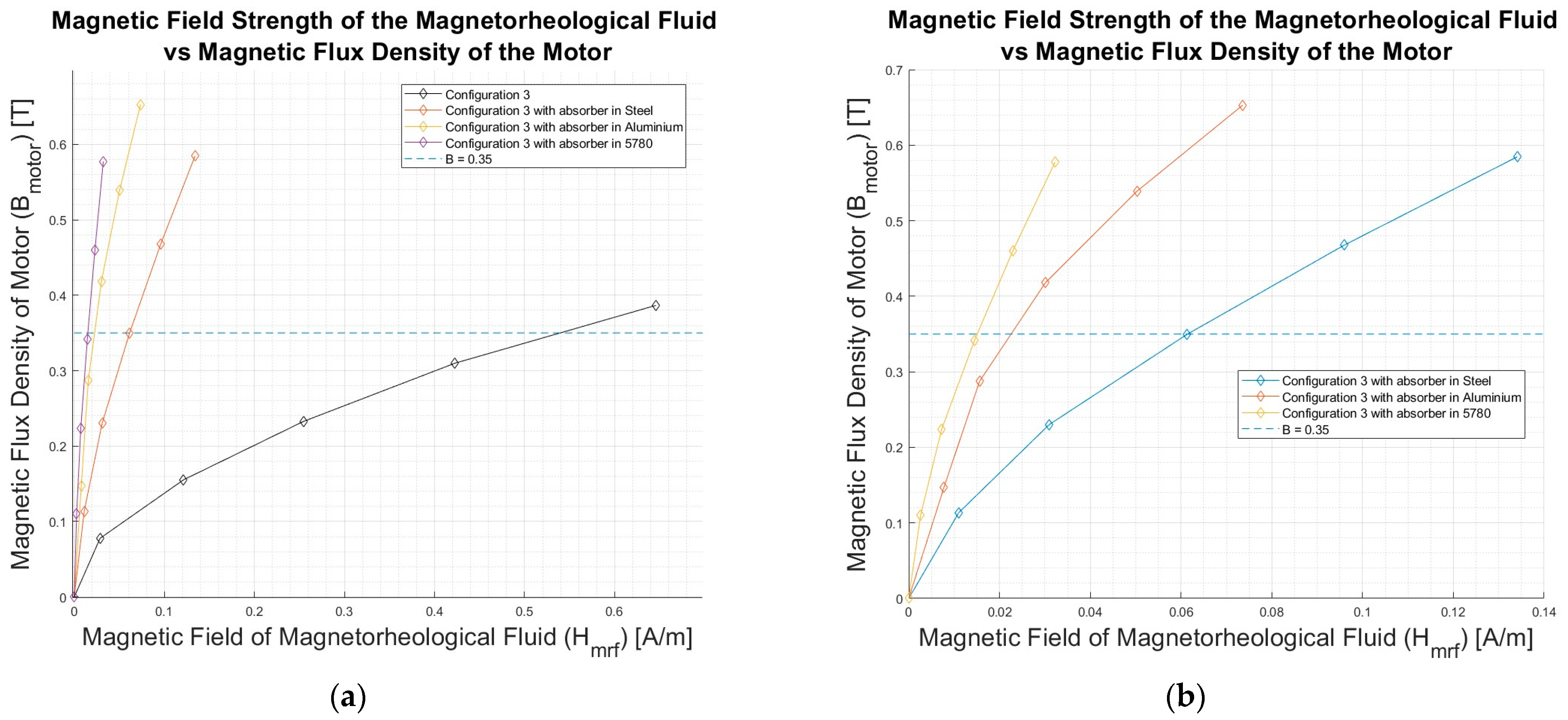
Configuration 3, equipped with a 6 mm steel absorber plate, exhibits slightly higher motor magnetic flux density compared to the normal configuration, attributed to the absorber’s proximity to the motor flux outlet. Notably, the magnetic field in the fluid decreases, indicating effective separation of the motor’s influence on the magnetorheological fluid’s magnetic field. The choice of absorber material, its thickness, composition, and distance contribute to these outcomes. The selected insulator, 5780-C5B from Holland Shielding Systems BV [39], composed of a magnetic powder and rubber composite, demonstrates efficient electromagnetic wave absorption and suppression capabilities.
Detailed material analyses, as presented in Table 7, reveal that the 5780-C5B absorber material outperforms steel and aluminium, reducing magnetic field density in the fluid. The comparative performance graph further emphasizes the superiority of the 5780-C5B absorber. B-H curve comparisons illustrate the absorbers’ similar characteristics, indicating a potential loss in magnetic qualities due to absorption, resulting in a high magnetic flux density ratio in the motor compared to the magnetic field strength in the fluid.
In Figure 15a,b, obtained by the results of Table 8 and Table 9, it is possible to note that the average magnetic flux density on the motor decreases by: 33.44% for the steel material, 43.16% for the aluminium material, and 32.18% for the 5780-C5B absorber material.
This is obtained by the comparison with the normal state of the brake, without the absorber, as seen in Table 5 and Table 6. Increasing the magnetic field strength makes slight changes to the flux density and the magnetic material is said to be saturated. This means that to produce a decrease in flux density a disproportionately large decrease in magnetic field strength is necessary. After the insertion of the absorber, the magnetic field strength on the MRF-132-DG decreases by 77.42% for the steel material, 61.58% for the aluminium material, and 78.35% for the 5780-C5B absorber material. In Figure 15b, the configuration with the absorber in 5790-C5B is linear. This trend occurs because the diminished influence of the magnetic field coming from the motor causes the fluid in a static state to lose magnetization and become more rigid. Similarly, in non-magnetic materials, the magnetization curve is a straight line passing through the origin.
6. Conclusions
This article investigates how magnetorheological brakes interact with electric motors. It examines them using a new analytical model, which differs from traditional designs by employing a simplified approach to understand their electromagnetic emissions. The brake design introduces a unique coil arrangement directly on its side housing, deviating from the traditional bobbin-coiled setup. On the other hand, the motor design explores four layouts, with a primary goal of minimizing magnetic field interference between the in-wheel motor and the brake, while remaining within the European directive limits. The two components were studied together through mathematical computations and various simulation analyses, which evaluated the impact of the motor’s magnetic field on the brake, leading to a non-traditional solution inspired by Helmholtz coil configurations. Using this solution, four potential motor–brake configurations are generated, and after thorough evaluation, the third configuration is selected. Simulations and numerical methods applied confirm its accuracy and viability for the intended application.
The behaviour analysed in this work is consistent with similar analyses in terms of FEA simulations of Helmholtz coils [40]. Furthermore, the results of the simulations are not only useful for underlining the effect of the magnetic emissions of the motor on the innovative braking system but also for correlating the Helmholtz coil similitude to real electromagnetic emissions. The simulation strategy in the present paper is also verified by comparing the obtained direction and strength of the magnetic flux to those found in various FEA studies [41]. In this study, a time- and cost-effective solution is represented, enabling the simulation of how the motor interacts with a brake without the need for designing the entire motor.
A comprehensive study in the fifth section addresses excessive electromagnetic fields using absorbers made of varied materials. Despite minimal interference, the importance of absorbers is highlighted considering potential alterations based on torque and fluid magnetization variations. The proposed unique MRB design requires experimental validation to affirm its effectiveness.
Future works could start from analysing the interaction between the motor and the brake during dynamic braking manoeuvres and while there is an electromagnetic emission from both the motor and the brake. Other advancements include developing a comprehensive multi-physics simulation for magnetic, fluid flow, structural, and heat analysis, followed by experimentally evaluating the innovative MRB design. This article unveils a novel MRB design, navigating optimization complexities, motor selection, and absorber considerations, contributing to the efficiency and resilience of MRBs in diverse operational scenarios, advancing innovation in the field.
Author Contributions
Conceptualization, G.I., H.d.C.P. and M.C.; Methodology, G.I. and H.d.C.P.; Software, G.I. and S.C.; Validation, G.I., H.d.C.P. and S.C.; Formal analysis, G.I., H.d.C.P., S.C. and M.C.; Investigation, G.I., H.d.C.P., S.C. and M.C.; Resources, M.C.; Data curation, G.I.; Writing—original draft, S.C.; Writing—review and editing, G.I., H.d.C.P. and M.C.; Visualization, H.d.C.P.; Supervision, M.C.; Project administration, M.C.; Funding acquisition, M.C. All authors have read and agreed to the published version of the manuscript.
Funding
This research received no external funding.
Data Availability Statement
All relevant data are reported in the article.
Conflicts of Interest
The authors declare no conflicts of interest.
References
- De Carvalho Pinheiro, H.; Messana, A.; Carello, M. In-wheel and on-board motors in BEV: Lateral and vertical performance comparison. In Proceedings of the 2022 IEEE International Conference on Environment and Electrical Engineering and 2022 IEEE Industrial and Commercial Power Systems Europe (EEEIC/I&CPS Europe), Prague, Czech Republic, 28 June–1 July 2022; pp. 1–6. [Google Scholar] [CrossRef]
- Imberti, G.; de Carvalho Pinheiro, H.; Carello, M. Impact of the Braking System Generated Pollutants on the Global Vehicle Emissions: A Review. In Proceedings of the ICESE 2023, Leuven, Belgium, 8–10 September 2023; Springer: Berlin/Heidelberg, Germany, 2023. [Google Scholar]
- Imberti, G. Regenerative Braking Effects on Pollutant Release and Zero-Emissions Brakes Technologies. Master’s Thesis, Politecnico di Torino, Turin, Italy, 2021. [Google Scholar]
- Dyke, S.J.; Spencer, B.F., Jr.; Sain, M.K.; Carlson, J.D. An experimental study of MR dampers for seismic protection. Smart Mater. Struct. 1998, 7, 693. [Google Scholar] [CrossRef]
- Brancati, R.; Di Massa, G.; Motta, C.; Pagano, S.; Petrillo, A.; Santini, S. A Test Rig for Experimental Investigation on a MRE Vibration Isolator. In The International Conference of IFToMM ITALY; Springer International Publishing: Cham, Switzerland, 2022. [Google Scholar] [CrossRef]
- Imberti, G.; de Carvalho Pinheiro, H.; Carello, M. Design of an Innovative Zero-Emissions Braking System for Vehicles. In Proceedings of the 2022 International Conference on Electrical, Computer, Communications and Mechatronics Engineer-ing, ICECCME, Male, Maldives, 16–18 November 2022. [Google Scholar] [CrossRef]
- de Carvalho Pinheiro, H.; Imberti, G.; Carello, M. Pre-Design and Feasibility Analysis of a Magneto-Rheological Braking System for Electric Vehicles; SAE Technical Paper; SAE Publications: Warrendale, PA, USA, 2023. [Google Scholar] [CrossRef]
- Fahem, M.E. Axial and Radial Flux Permanent Magnet Machines—What Is the Difference? EMWORKS, 2020. Available online: https://www.emworks.com/blog/electromechanical/axial-and-radial-flux-permanent-magnet-machines-what-is-the-difference (accessed on 6 June 2023).
- Emrax. Emrax 348, Motor Installation and Maintenance Manual; EMRAX d.o.o: Kamnik, Slovenia, 2020. [Google Scholar]
- Woolmer, T.; McCulloch, M. Analysis of the Yokeless and Segmented Armature Machine. In Proceedings of the 2007 IEEE International Electric Machines & Drives Conference, Antalya, Turkey, 3–5 May 2007. [Google Scholar]
- European Union. Commission Communication in the Framework of the Implementation of Directive 2006/95/EC of the European Parliament and of the Council on the Harmonisation of the Laws of Member States Relating to Electrical Equipment Designed for Use within Certain Voltag; European Union: Brussels, Belgium, 2015. [Google Scholar]
- AIS-004; (Part 3): Automotive Vehicles–Requirements for Electromagnetic Compatibility, Central Motor Vehicle Rules—Technical Standing Committee. The Automotive Research Association of India: Pune, India, 2009.
- European Parliament. Directive 2014/30/EU of the European Parliament; European Union: Brussels, Belgium, 2014; Available online: https://eur-lex.europa.eu/legal-content/EN/TXT/?uri=CELEX:32014L0030#d1e32-97-1 (accessed on 11 September 2018).
- Halbach, K. Design of permanent multipole magnets with oriented rare earth cobalt material. Nucl. Instrum. Methods 1980, 169, 1–10. [Google Scholar] [CrossRef]
- Halbach, K. Applications of Permanent Magnets in Accelerators and Electron Storage Rings. J. Appl. Phys. 1985, 57, 3605–3608. [Google Scholar] [CrossRef]
- SDM Magnetics. Brief Introduction to Halbach Array. Techtalk, 2022. Available online: https://www.magnet-sdm.com/2018/10/30/halbach-array/ (accessed on 12 March 2024).
- Abbott, J.J. Parametric design of tri-axial nested Helmholtz coils. Rev. Sci. Instrum. 2015, 86, 054701. [Google Scholar] [CrossRef] [PubMed]
- Sundarnath, J.K.; Resendiz, E.M.; Kuravi, S. Particle Arrangement using External Magnetic Field and its effect on Pressure Drop in a Tightly Packed Ferromagnetic Porous Bed. Powder Technol. 2020, 375, 275–283. [Google Scholar] [CrossRef]
- Butta, M.; Ripka, P.; Infante, G.; Badini-Confalonieri, G.A. Magnetic microwires with field induced helical anisotropy for coil-less fluxgate. IEEE Trans. Magn. 2010, 46, 2562–2565. [Google Scholar] [CrossRef]
- Sadiq, U.A.; Oluyombo, O.W. Optimization Design and Characterization of Helmholtz Coils. J. Inf. Eng. Appl. 2019, 9, 4. [Google Scholar]
- Daron, B.B.; Jonathan, E.; Madsen, M.J. Magnetic field mapping. Wabash J. Phys. 2015, 4, 1–13. [Google Scholar]
- Jiang, C.; Gao, P.; Yang, X.; Ji, D.; Sun, J.; Yang, Z. Helmholtz Coils Based WPT Coupling Analysis of Temporal Interference Electrical Stimulation System. Appl. Sci. 2022, 12, 9832. Available online: https://www.mdpi.com/2076-3417/12/19/9832 (accessed on 30 May 2023). [CrossRef]
- Scientific Instruments GmbH. Definitions Used for Helmholtz Coils; Scientific Instruments GmbH: Gilching, Germany, 2021; Available online: https://www.si-gmbh.de/wp-content/uploads/2021/06/DefinitionsUsedForHelmholtzCoils.pdf (accessed on 12 March 2024).
- Fufaev, A. Derivation, Magnetic Field of a Helmholtz Coil. 2021. Available online: https://en.universaldenker.org/arguments/326#calculate-the-magnetic-field-of-the-first-helmholtz-coil (accessed on 20 June 2023).
- Holmes, N.; Tierney, T.M.; Leggett, J.; Boto, E.; Mellor, S.; Roberts, G.; Hill, R.M.; Shah, V.; Barnes, G.R.; Brookes, M.J.; et al. Balanced, bi-planar magnetic field and field gradient coils for field compensation in wearable magnetoencephalography. Sci. Rep. 2019, 9, 14196. [Google Scholar] [CrossRef] [PubMed]
- Rajnak, M.; Wu, Z.; Dolnik, B.; Paulovicova, K.; Tothova, J.; Cimbala, R.; Kurimský, J. Magnetic Field Effect on Thermal, Dielectric, and Viscous Properties of a Transformer Oil-Based Magnetic Nanofluid, Peter Kopcansky, Lars Wadsö, Milan Timko. Energies 2019, 12, 4532. [Google Scholar] [CrossRef]
- Bruneel, J. Axial Flux Motor vs Radial Flux Motor: A Focus on Magnetic Field Orientation. TRAXIAL. 04 04 2022. Available online: https://traxial.com/blog/electric-motor-design-magnetic-field-orientation/ (accessed on 5 April 2023).
- Akatsu, K.; Wakui, S. A comparison between axial and radial flux PM motor by optimum design method from the required output NT characteristics. COMPEL-Int. J. Comput. Math. Electr. Electron. Eng. 2006, 25, 496–509. [Google Scholar] [CrossRef]
- Cary, N. Designing with MR Fluid; Lord Corporation Engineering: Cary, NC, USA, 1999. [Google Scholar]
- Özsoy, K.; Usal, M.R. A mathematical model for the magnetorheological materials and magneto reheological devices. Eng. Sci. Technol. Int. J. 2018, 21, 1143–1151. [Google Scholar] [CrossRef]
- Lord, C. MRF-132DG Magneto-Rheological Fluid; Lord Technical Data; Lord Corporation Engineering: Cary, NC, USA, 2023. [Google Scholar]
- Kumbhar, B.K.; Patil, S.R.; Sawant, S.M. Synthesis and characterization of magneto-rheological (MR) fluids. Eng. Sci. Technol. Int. J. 2015, 18, 432–438. [Google Scholar]
- AspenCore Inc. Magnetic Hysteresis. Electronics Tutorials 2023. Available online: https://www.electronics-tutorials.ws/electromagnetism/magnetic-hysteresis.html (accessed on 20 June 2023).
- ASTM International. Annual Book of ASTM Standards; ASTM International: West Conshohocken, PA, USA, 2005. [Google Scholar]
- Karakoc, K. Design of a Magnetorheological Brake System Based on Magnetic Circuit Optimization. Master’s Thesis, Bogazici University, Istanbul, Turkey, 2007. [Google Scholar]
- Taiyo. Radio Wave Absorber MICROSOBER® for a Clean Electromagnetic Environment. Taiyo Wire Cloth Co. 22 March 2022. Available online: https://www.twc-net.com/blog/2022/post-688.html (accessed on 30 June 2023).
- Kotsuka, Y. Electromagnetic Wave Absorbers: Detailed Theories and Applications; John Wiley & Sons, Inc.: Hoboken, NJ, USA, 2019. [Google Scholar]
- Mušič, B.; Žnidaršič, A.; Venturini, P.; Domžale, H. Materials, electromagnetic absorbing. Inf. MIDEM 2011, 41, 86–91. [Google Scholar]
- Holland Shielding Systems, BV. 5780-C-EMI Flexible Absorber Sheets, Technical Datasheet. Lipsweg 124, Netherlands, 19-9-2017. Available online: https://hollandshielding.com/en/flexible-emi-absorber-sheets (accessed on 12 March 2024).
- Zhang, W.; Yang, S.-L. Analysis and verification of the Helmholtz field coil electromagnetic based on finite element method. Energy Mech. Eng. 2016, 702–711. [Google Scholar] [CrossRef]
- Tan, L.; Eldin, K.; Elnail, I.; Ju, M.; Huang, X. Comparative Analysis and Design of the Shielding Techniques in WPT Systems for Charging EVs. Energies 2019, 12, 2115. [Google Scholar] [CrossRef]
Figure 1.
(a) Magnetic field configuration magnet array; (b) Simulation Analysis of a Halbach Array Model [16].
Figure 1.
(a) Magnetic field configuration magnet array; (b) Simulation Analysis of a Halbach Array Model [16].
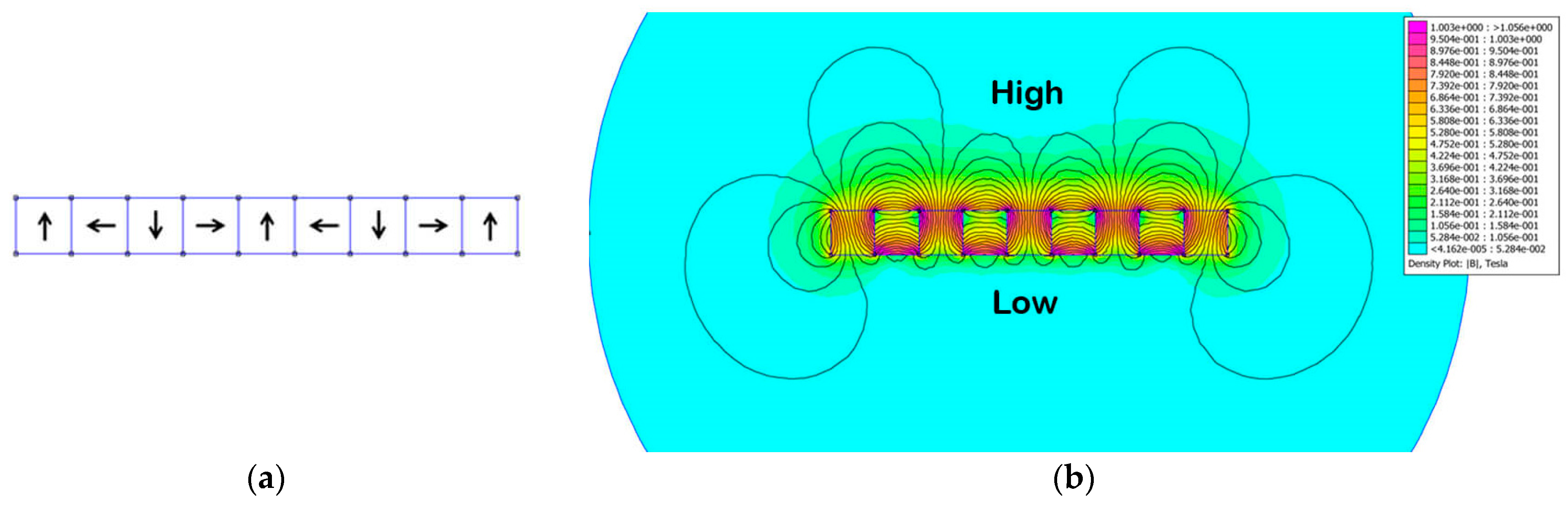
Figure 2.
Magnetic field simulation of the Helmholtz coil comprising two 200 mm, 500500-turnectric coils in air [18]: (a) Top view; (b) Side view.
Figure 2.
Magnetic field simulation of the Helmholtz coil comprising two 200 mm, 500500-turnectric coils in air [18]: (a) Top view; (b) Side view.

Figure 3.
Coil configuration and simulation in two different directions [25]: (a) Same direction; (b) Opposite direction.
Figure 3.
Coil configuration and simulation in two different directions [25]: (a) Same direction; (b) Opposite direction.

Figure 4.
Brake geometry: (a) Brake section; (b) Brake parts: 1. MR Fluid Selection (blue), 2. Coils (purple), 3. Bobbins (red), 4. Lip Seals (black), 5. Rotor (light green), 6. Stator (dark green), 7. Cover (grey).
Figure 4.
Brake geometry: (a) Brake section; (b) Brake parts: 1. MR Fluid Selection (blue), 2. Coils (purple), 3. Bobbins (red), 4. Lip Seals (black), 5. Rotor (light green), 6. Stator (dark green), 7. Cover (grey).
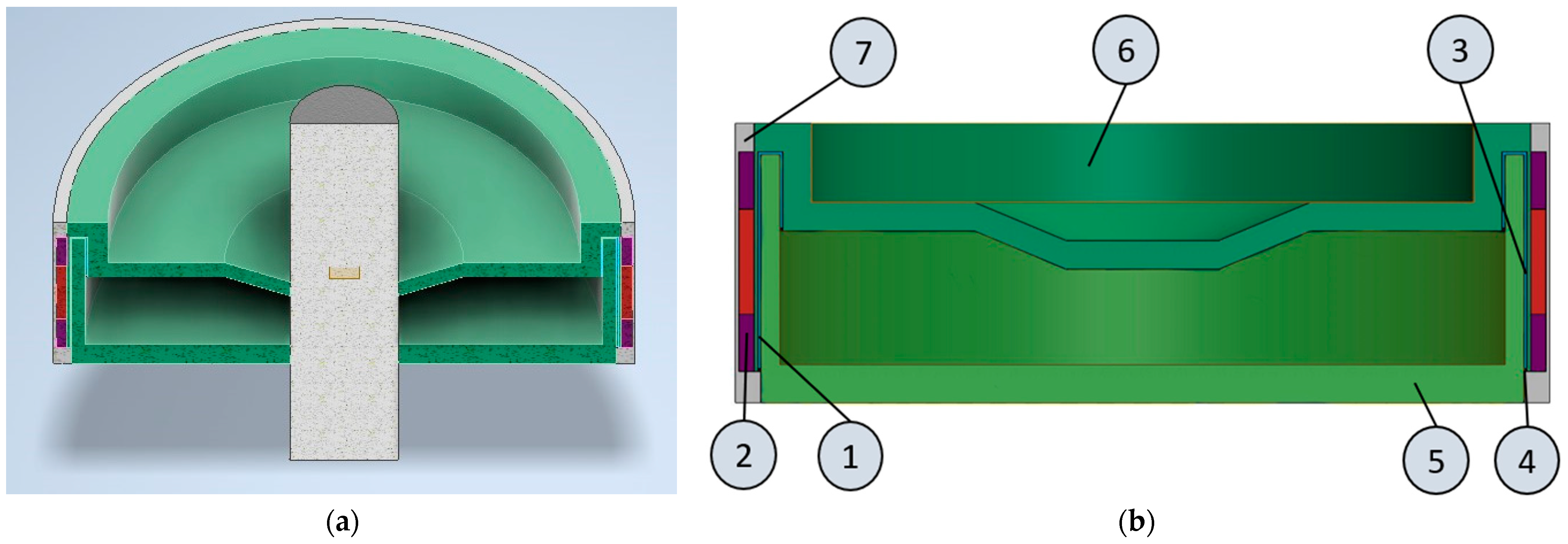
Figure 5.
B-H curve for MRF [31].
Figure 5.
B-H curve for MRF [31].
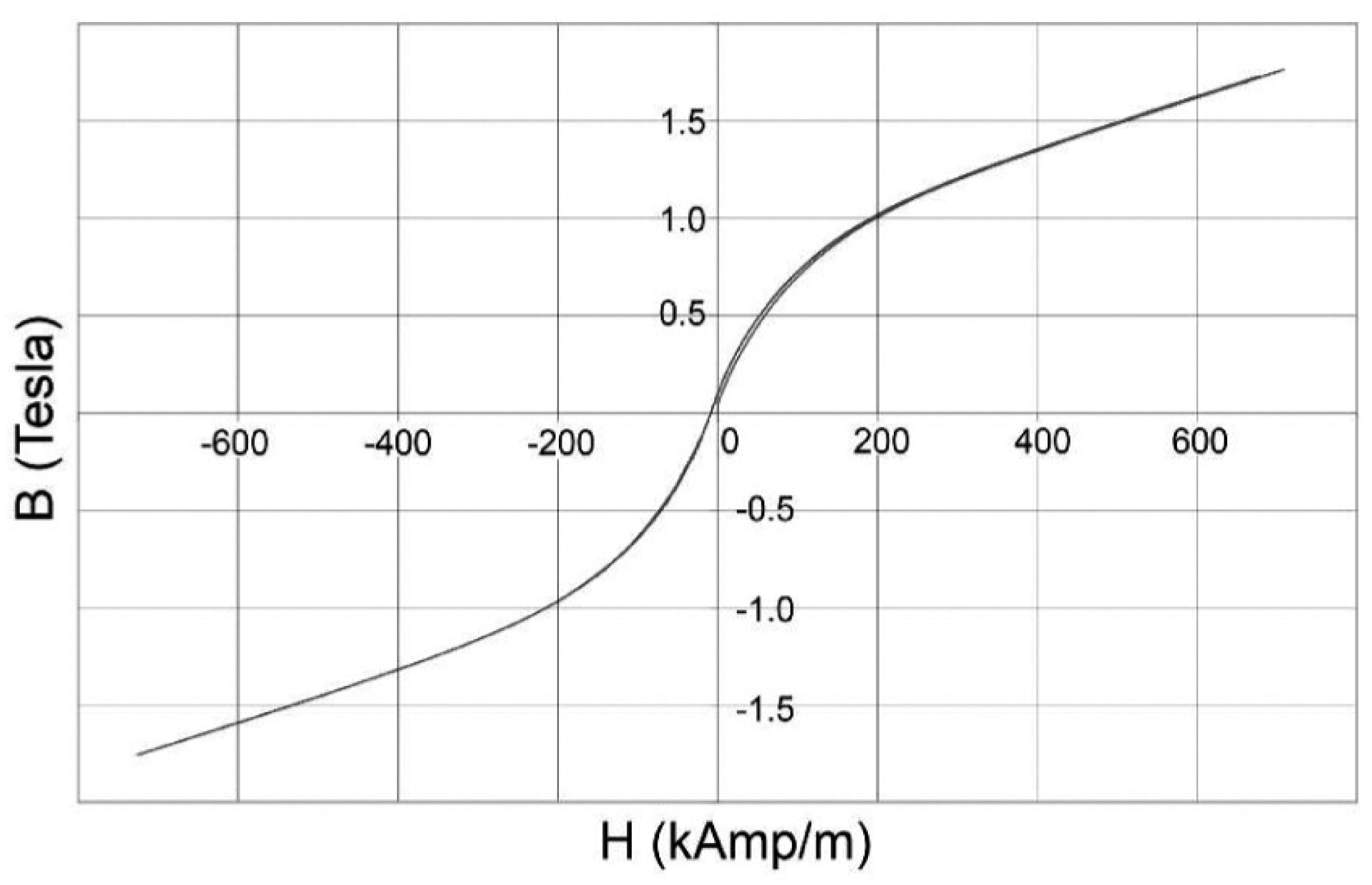
Figure 6.
Configuration simulation at : (a) Coil configuration side view; (b) Influence of coil configuration on the brake; (c) Close-up lip view.
Figure 6.
Configuration simulation at : (a) Coil configuration side view; (b) Influence of coil configuration on the brake; (c) Close-up lip view.
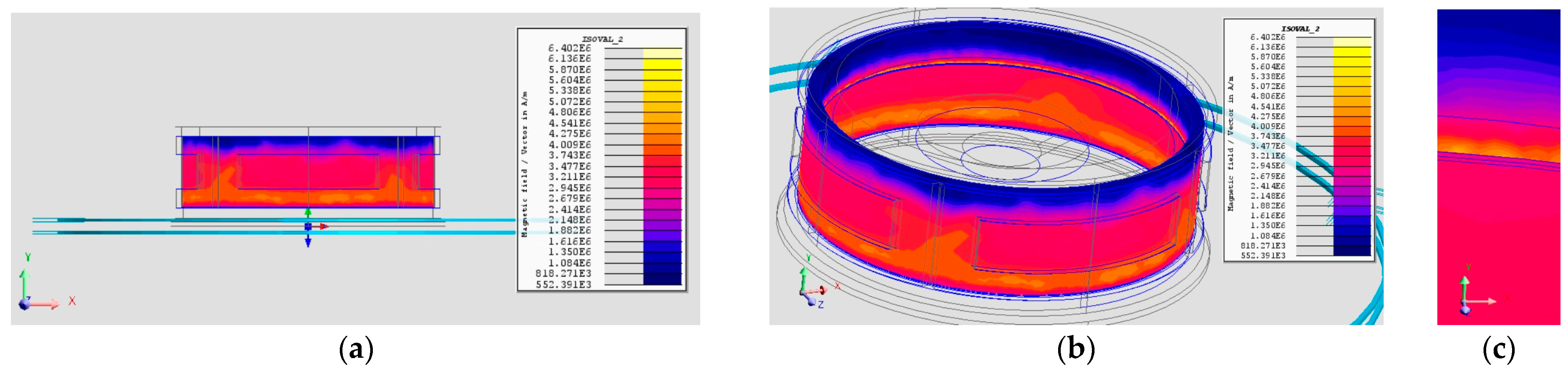
Figure 7.
Configuration 2 simulation at : (a) Coil configuration side view; (b) Influence of coil configuration on the brake; (c) Close-up lip view.
Figure 7.
Configuration 2 simulation at : (a) Coil configuration side view; (b) Influence of coil configuration on the brake; (c) Close-up lip view.
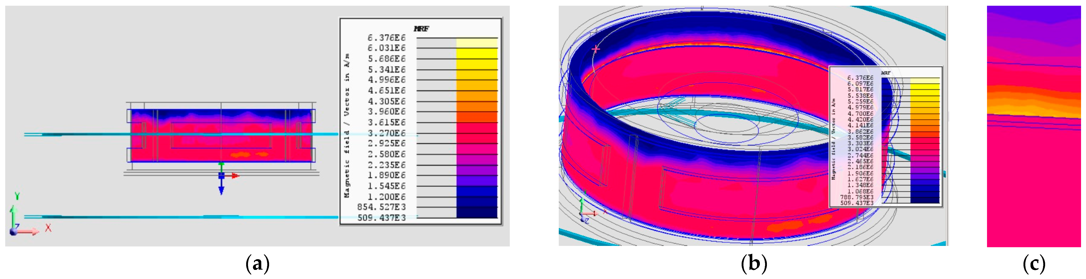
Figure 8.
Configuration 3 simulation at k = 1: (a) Coil configuration side view; (b) Influence of coil configuration on the brake; (c) Close-up lip view.
Figure 8.
Configuration 3 simulation at k = 1: (a) Coil configuration side view; (b) Influence of coil configuration on the brake; (c) Close-up lip view.
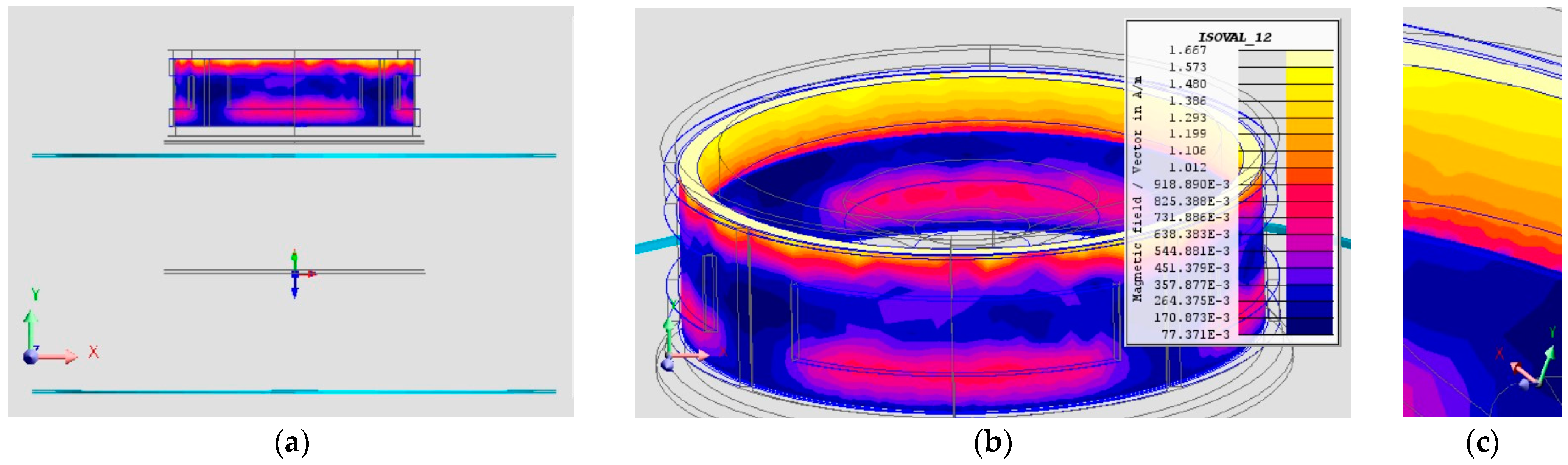
Figure 9.
Configuration 3 simulation at : (a) Coil configuration side view; (b) Influence of coil configuration on the brake; (c) Close-up lip view.
Figure 9.
Configuration 3 simulation at : (a) Coil configuration side view; (b) Influence of coil configuration on the brake; (c) Close-up lip view.

Figure 10.
Configuration 4 simulation at : (a) Coil configuration side view; (b) Influence of coil configuration on the brake; (c) Close-up lip view.
Figure 10.
Configuration 4 simulation at : (a) Coil configuration side view; (b) Influence of coil configuration on the brake; (c) Close-up lip view.
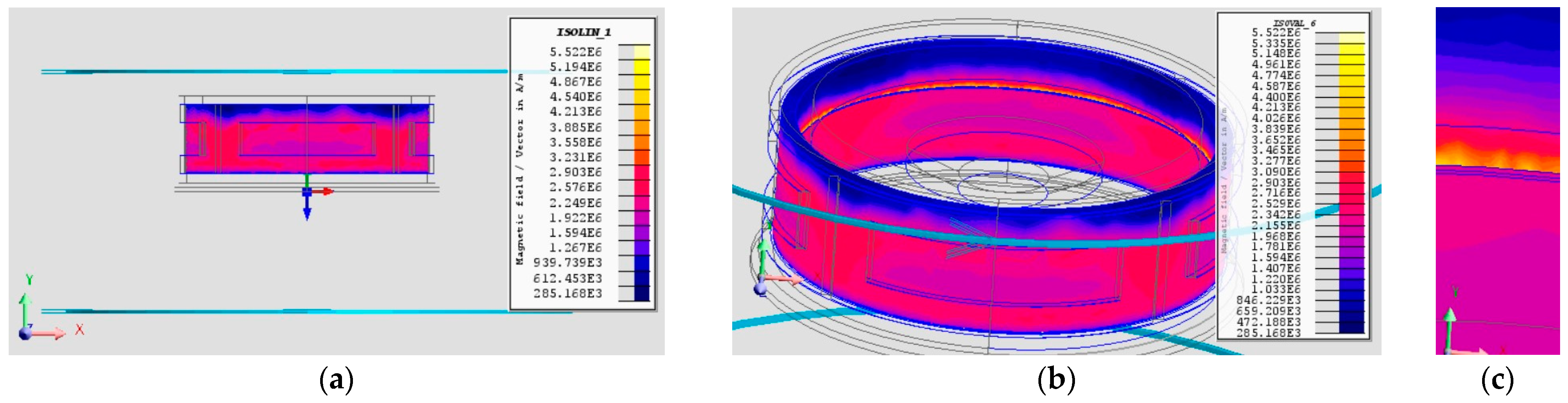
Figure 11.
The four configurations of the Helmholtz coil: (a) Configuration 1; (b) Configuration 2; (c) Configuration 3; (d) Configuration 4.
Figure 11.
The four configurations of the Helmholtz coil: (a) Configuration 1; (b) Configuration 2; (c) Configuration 3; (d) Configuration 4.
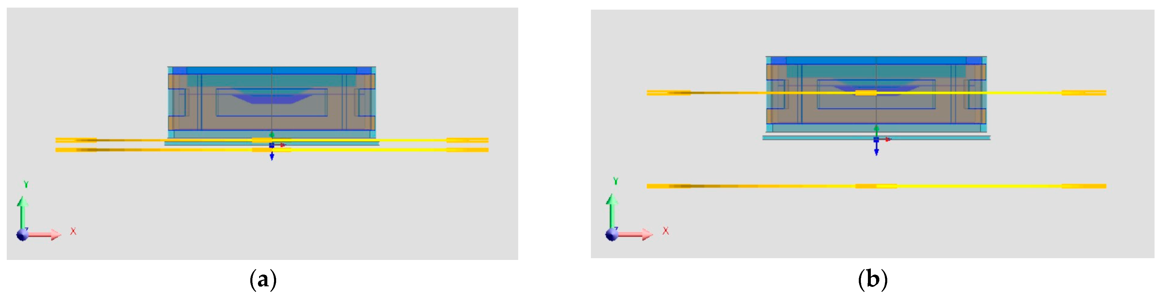
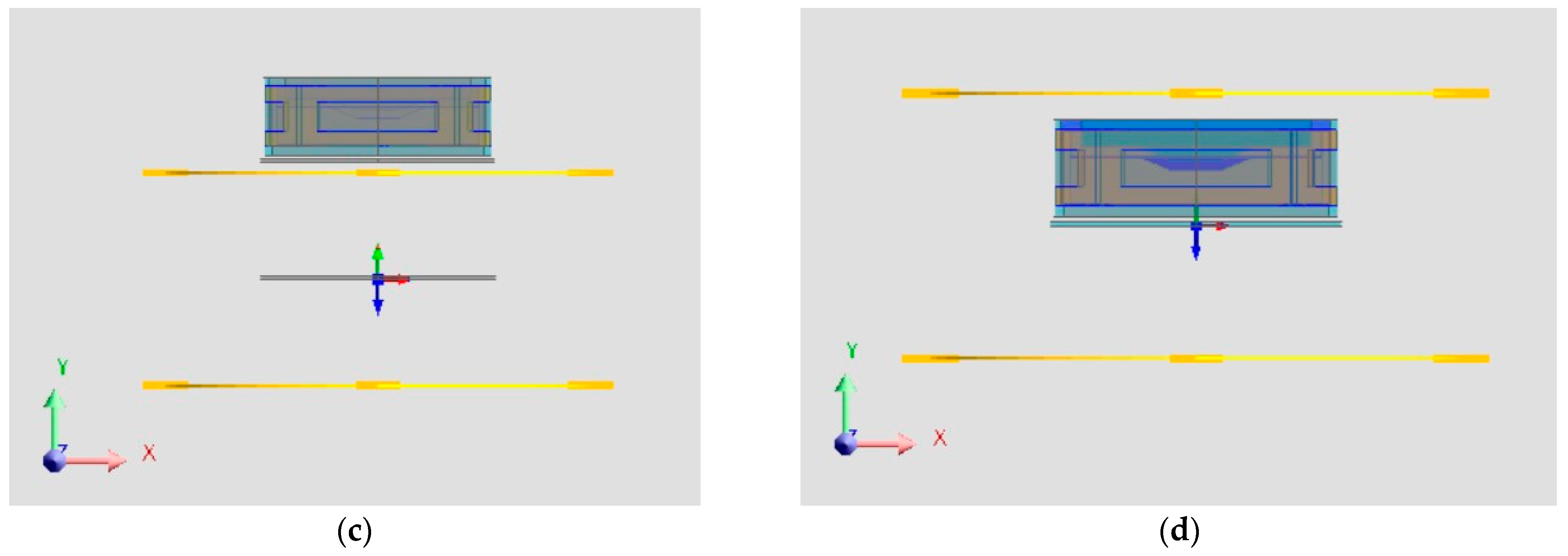
Figure 12.
Magnetic Flux Density of the motor averages vs. Magnetic Field of the Motor: (a) B-H curves of all configurations; (b) Zoomed-in B-H curves of all configurations.
Figure 12.
Magnetic Flux Density of the motor averages vs. Magnetic Field of the Motor: (a) B-H curves of all configurations; (b) Zoomed-in B-H curves of all configurations.
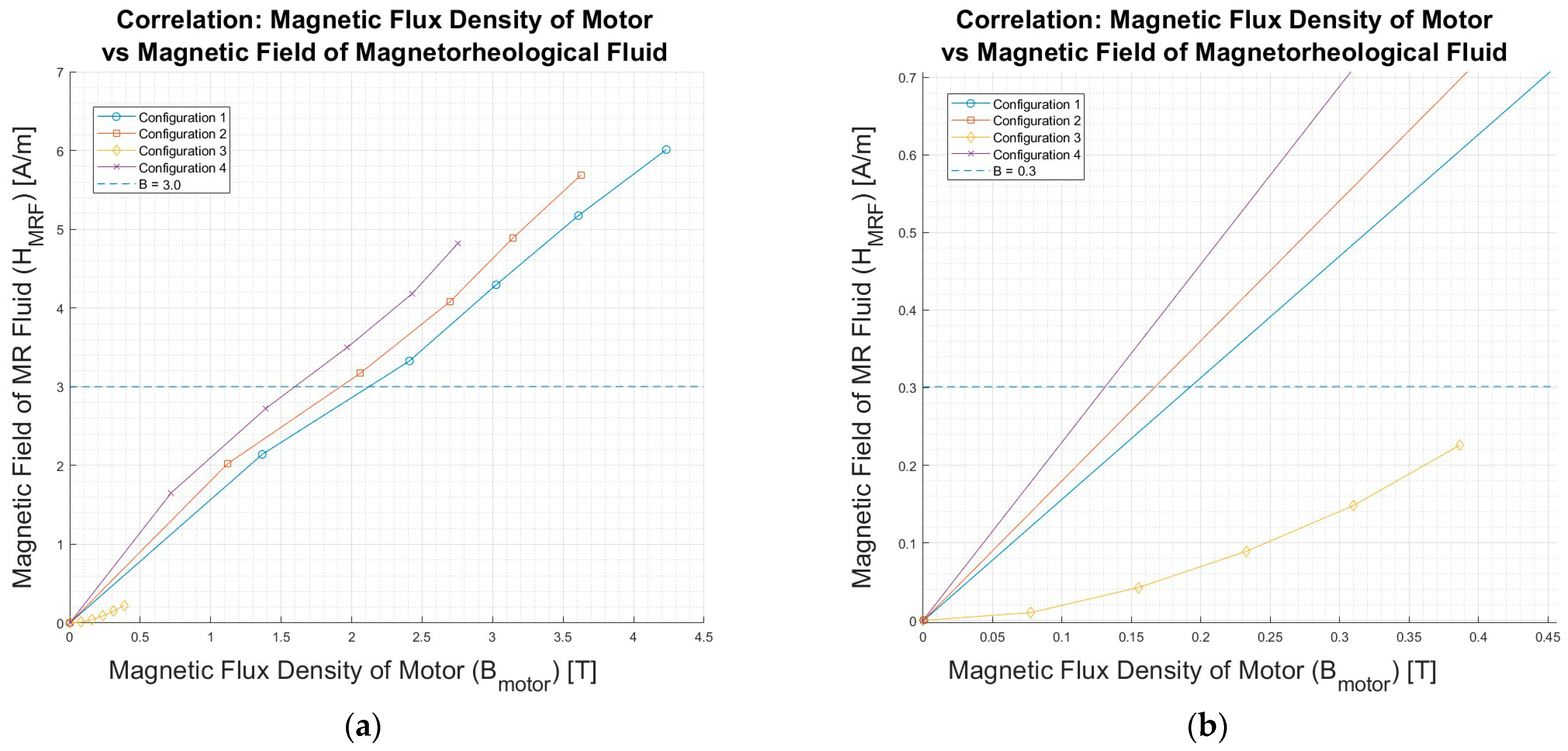
Figure 13.
Magnetic Flux Density of the motor averages vs. Magnetic Field of the MRF: (a) B-H curves of all configurations; (b) B-H curves of Configuration 3.
Figure 13.
Magnetic Flux Density of the motor averages vs. Magnetic Field of the MRF: (a) B-H curves of all configurations; (b) B-H curves of Configuration 3.
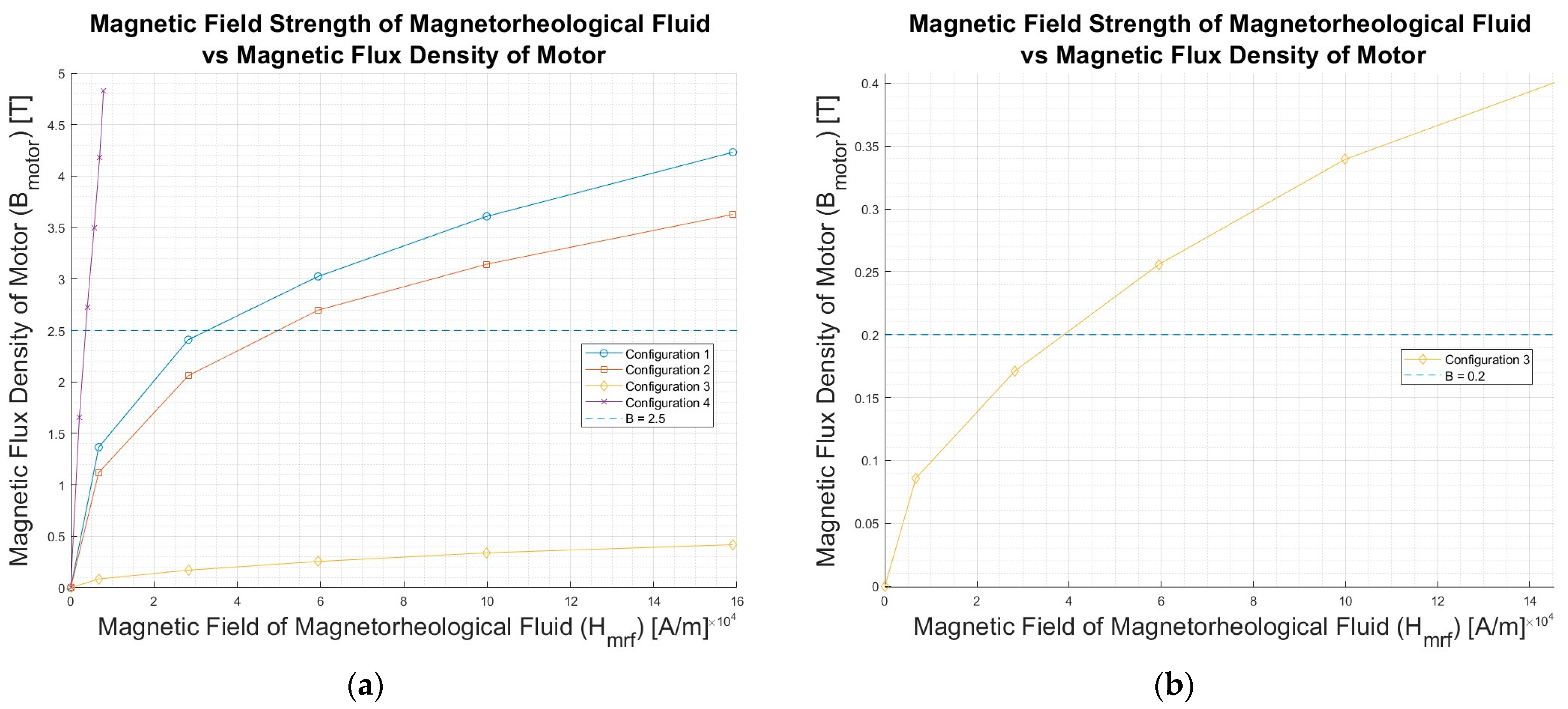
Figure 14.
Magnetic field influence on a metal object and on a magnetic sheet [36]: (a) metal object without the absorber; (b) metal object after the insertion of the absorber.
Figure 14.
Magnetic field influence on a metal object and on a magnetic sheet [36]: (a) metal object without the absorber; (b) metal object after the insertion of the absorber.
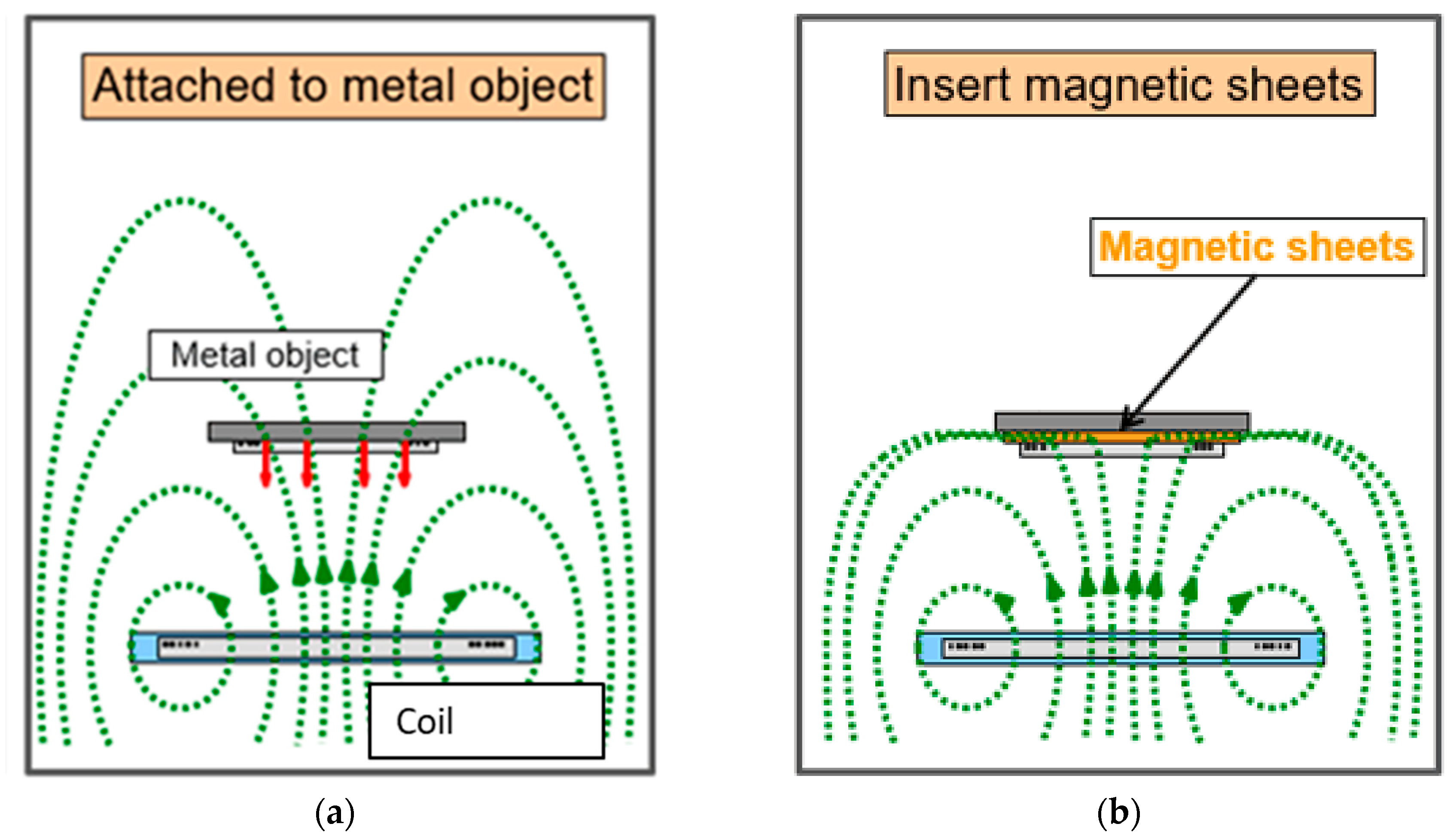
Figure 15.
Magnetic field strength of MRF-132-DG vs. Magnetic flux density on Configuration 3: (a) Comparison of B-H curves between three absorbers; (b) Comparison of B-H curves with and without the absorber.
Figure 15.
Magnetic field strength of MRF-132-DG vs. Magnetic flux density on Configuration 3: (a) Comparison of B-H curves between three absorbers; (b) Comparison of B-H curves with and without the absorber.

Table 1.
Geometry of Helmholtz coil data.
| Character | Name | Values | ||
|---|---|---|---|---|
| R | Coil radius [m] | 0.40 | ||
| d/2 | Half distance from the centre [m] | 0.01 | 0.09 | 0.20 |
| d | Distance from the centre [m] | 0.02 | 0.18 | 0.40 |
| A | Rectangular coil section area [] | |||
| N | Number of turns per coil | 100 | ||
| ρ | Resistivity [Wm] | |||
| FF | Fill factor [0 < Sf < 1] | 0.71 | ||
| V | Volume of the coil [] | |||
| Req | Equivalent resistance [W] | 24.07 | ||
| k | Helmholtz coil constant | |||
| MRF-132-DG | |
|---|---|
| Initial viscosity [Pa s] (at 25 °C) | 0.2–0.5 |
| Density [g/] | 2.95–3.15 |
| Magnetic field strength [kA/m] | 150–250 |
| Yield point [kPa] | 50–100 |
| Reaction time [ms] | 15–25 |
| Operating temperature [°C] | −40 to +130 |
| Typical supply voltage [V] | 2–25 |
| Typical current intensity [A] | 1–2 |
Table 3.
Material properties.
| Magnetic Properties | Aluminium | Copper | Steel | MRF-132-DG |
|---|---|---|---|---|
| Initial relative permeability | 1 | 1 | 2500 | 3.798 |
| Saturation magnetization [T] | - | - | 2.5 | 2.1 |
| Knee adjusting coefficient | - | - | 0.5 | 0.4 |
| Thermal conductivity [Wm−1K−1] | 0.52 | 0.92 | - | - |
| Saturation flux density [T] | - | - | 1.55 | 1.65 |
Table 4.
Average values needed for the calculation.
| MRF-132-DG | Motor (Steel) | |
|---|---|---|
| Permeability [h/m] | 3.798 | 2500 |
| Cross sectional area A [] | 0.00042 | 0.0012 |
| Average magnetic flux density B [T] | - | 0.1932 |
| Average magnetic field H [A/m] | - |
Table 5.
Magnetic field of the MRF for each configuration [A/m].
| Magnetic Field of the MRF [A/m] | ||||
|---|---|---|---|---|
| k | Configuration 1 | Configuration 2 | Configuration 3 | Configuration 4 |
| 0.03 | ||||
| 2.14 | 2.02 | 0.01 | ||
| 3.32 | 3.17 | 0.04 | ||
| 4.29 | 4.08 | 0.09 | ||
| 5.17 | 4.89 | 0.15 | ||
| 6.01 | 5.69 | 0.23 | ||
Table 6.
Magnetic flux density of the motor for each configuration [T].
| Magnetic Flux density of the Motor [T] | ||||
|---|---|---|---|---|
| k | Configuration 1 | Configuration 2 | Configuration 3 | Configuration 4 |
| 6.19 | ||||
| 1.37 | 1.12 | 0.08 | 1.65 | |
| 2.41 | 2.06 | 0.16 | 2.72 | |
| 4.29 | 2.70 | 0.23 | 3.50 | |
| 3.02 | 3.14 | 0.31 | 4.18 | |
| 3.61 | 3.63 | 0.39 | 4.83 | |
Table 7.
Properties of 5780-C absorber.
| 5780-C5B Absorber | |
|---|---|
| Material | Magnetic powder + rubber |
| Initial relative permeability | 250 |
| Saturation magnetization [T] | Around 2 |
| Knee adjusting coefficient | 0.5 |
| Mass density [kg/] | 4.4 |
| Surface resistance |
Table 8.
Comparison of B values for configuration 3 with and without absorber.
| Configuration 3—Magnetic Flux Densities on the Motor B [T] | ||||
|---|---|---|---|---|
| Coefficient k | Without Absorber | With Absorber in | ||
| Steel | Aluminium | 5780-C5B | ||
| 0.08 | 0.11 | 0.15 | 0.11 | |
| 0.16 | 0.23 | 0.29 | 0.22 | |
| 0.23 | 0.35 | 0.42 | 0.34 | |
| 0.31 | 0.47 | 0.54 | 0.46 | |
| 0.39 | 0.58 | 0.65 | 0.58 | |
Table 9.
Comparison of H values for configuration 3 with and without absorbers.
| Configuration 3—Magnetic Field on the MRF-132-DG H [A/m] | ||||
|---|---|---|---|---|
| Coefficient k | Without Absorber | With Absorber in: | ||
| Steel | Aluminium | 5780-C5B | ||
Disclaimer/Publisher’s Note: The statements, opinions and data contained in all publications are solely those of the individual author(s) and contributor(s) and not of MDPI and/or the editor(s). MDPI and/or the editor(s) disclaim responsibility for any injury to people or property resulting from any ideas, methods, instructions or products referred to in the content. |
© 2024 by the authors. Licensee MDPI, Basel, Switzerland. This article is an open access article distributed under the terms and conditions of the Creative Commons Attribution (CC BY) license (https://creativecommons.org/licenses/by/4.0/).
Share and Cite
MDPI and ACS Style
Caushaj, S.; Imberti, G.; de Carvalho Pinheiro, H.; Carello, M. Electromagnetic Interaction Model between an Electric Motor and a Magnetorheological Brake. Designs 2024, 8, 25. https://doi.org/10.3390/designs8020025
AMA Style
Caushaj S, Imberti G, de Carvalho Pinheiro H, Carello M. Electromagnetic Interaction Model between an Electric Motor and a Magnetorheological Brake. Designs. 2024; 8(2):25. https://doi.org/10.3390/designs8020025
Chicago/Turabian StyleCaushaj, Sidorela, Giovanni Imberti, Henrique de Carvalho Pinheiro, and Massimiliana Carello. 2024. "Electromagnetic Interaction Model between an Electric Motor and a Magnetorheological Brake" Designs 8, no. 2: 25. https://doi.org/10.3390/designs8020025