
Scanning Technologies to Building Information Modelling: A Review


1
Applied Geotechnologies Group, School of Mining and Energy Engineering, University of Vigo, 36310 Vigo, Spain
2
ICT & Innovation Department, Ingeneria Insitu, 36310 Vigo, Spain
*
Author to whom correspondence should be addressed.
Infrastructures 2022, 7(4), 49; https://doi.org/10.3390/infrastructures7040049
Submission received: 25 February 2022
/
Revised: 19 March 2022
/
Accepted: 28 March 2022
/
Published: 30 March 2022
(This article belongs to the Section Smart Infrastructures)
Abstract
:Building information modelling (BIM) is evolving significantly in the architecture, engineering and construction industries. BIM involves various remote-sensing tools, procedures and standards that are useful for collating the semantic information required to produce 3D models. This is thanks to LiDAR technology, which has become one of the key elements in BIM, useful to capture a semantically rich geometric representation of 3D models in terms of 3D point clouds. This review paper explains the ‘Scan to BIM’ methodology in detail. The paper starts by summarising the 3D point clouds of LiDAR and photogrammetry. LiDAR systems based on different platforms, such as mobile, terrestrial, spaceborne and airborne, are outlined and compared. In addition, the importance of integrating multisource data is briefly discussed. Various methodologies involved in point-cloud processing such as sampling, registration and semantic segmentation are explained in detail. Furthermore, different open BIM standards are summarised and compared. Finally, current limitations and future directions are highlighted to provide useful solutions for efficient BIM models.
1. Introduction
In recent decades, building information modelling (BIM) has become one of the most significant emerging technologies in the architecture, engineering and construction (AEC) industries. The applications of BIM are gaining popularity in numerous fields such as transport infrastructures [1,2,3,4], 3D city modelling [5,6], economic systems [7,8] and mechanical, electrical and plumbing (MEP) fields [9,10,11]. BIM is defined as an intelligent 3D model that provides information about the assets during the project lifecycle, which is useful to plan, design, create and operate infrastructures and buildings more efficiently. BIM aims to have benefits like cost reduction and control, coordination and collaboration, better customer service, production quality and easy maintenance [11,12]. In this way, it saves time and gives a complete picture to the project team so that they can easily maintain and operate buildings and unravel any complexities that might arise. Despite the benefits, some challenges are still faced, such as interoperability, big data and a lack of automatic processes. Therefore, standard platforms for integration and standardisation are necessary for developing BIM to predict and analyse the future stages of as-built models or new building models. For successful BIM implementation, high-performing measurement, sufficient attribute information and accurate graphics are the most important factors. Laser-scanning advancements have increased the usefulness and accessibility of 3D measurement devices in BIM. These sensors make direct measurements from the sensor to objects in the surroundings and are extensively employed in BIM models. Using attributes of the objects in the model, BIM can indicate what needs to be measured. It assists in determining the dimensions of any object by measuring points within the scanning range. The vast volume of data generated by 3D-measurement laser scanners needs to be processed and transmitted efficiently. It is, therefore, necessary to have a thorough understanding of point-cloud processing algorithms and BIM standards. At present, LiDAR is seen as a robust method to collect 3D measurement points more efficiently. The process of capturing a physical site or space using scan data, from the air or from the ground, to develop an intelligent 3D model by employing BIM software, is known as ‘Scan to BIM’ [13,14].
General Framework: Scan to BIM
The Scan to BIM process is used to produce the as-built model of an asset that tends to suffer from a lack of information, outdated plans or incomplete documentation. This is where the Scan to BIM plays a vital role. This process takes point clouds as an input and outputs a final 3D reconstruction model where all the assets are classified or labelled. The framework design consists of the following steps:
- Data capture: Laser-scanner technologies play a fundamental role in the construction of an as-built BIM. The data are captured in the form of raw point clouds. There are also other methods to generate point clouds such as photogrammetry. However, this method is time-consuming and its accuracy degrades when surveying large areas. In this step, certain points must be clear—for example, scanning parameters, point clouds’ resolution, and their density—with appropriate equipment selected according to the user’s application.
- Semantic segmentation: Once the registration of all the scans is completed, it is combined into a single 3D point cloud. Then, assets are detected and classified, which can be further processed in BIM software.
- BIM model: In the last step, standards such as IFC and gbXML are applied to exchange the information between software applications for BIM.
To our knowledge, this is the first review that focuses on the entire chain of the Scan to BIM framework. Existing research focuses on one of three topics: point-cloud processing, 3D reconstruction or building information modelling [15,16,17]. However, none of these studies has given a comprehensive review of the Scan to BIM framework. Recently, the authors in [17] published a survey based on the 3D reconstruction of buildings, which mainly focused on data acquisition and processing techniques. In contrast, our paper gives detailed information regarding scanning technologies, point-cloud data-processing techniques for sampling, registration, and semantic segmentation, as well as the open standards used in BIM, which will be useful for new researchers. This will help academics and even construction companies to comprehend the challenges they face and gain useful insights into future trends.
2. Research Methodology
Figure 1 outlines the structure of the review paper. In the first stage, we focus on the importance of 3D point clouds obtained from LiDAR and photogrammetry and outline how LiDAR data is useful in BIM. In the next stage, LiDAR systems based on different platforms are outlined and compared. Additionally, the importance of combining multisource data from different LiDAR and photogrammetry methods is discussed. In stage 3, various point-cloud processing methods are explained and major challenges of traditional and deep-learning approaches are outlined, which can be critical for developing the Scan to BIM framework. Stage 4 defines the interoperability and open standards for Scan to BIM. The last stage concludes and identifies future research directions.
To carry out a comprehensive review, Elsevier Scopus and Google Scholar were mainly used. Table 1 illustrates the literature search keywords. The keyword search was carried out utilising the “AND” and “OR” Boolean operators to combine keywords, for example, “Scan to BIM” AND “point clouds”, “registration” AND “deep learning”.
Furthermore, the numbers of different document types sampled—articles, conference papers, reviews, book chapters and survey papers—are specified in Figure 2. There are 91 article papers and 84 conference papers, followed by 15 review papers, 1 book chapter and 1 short review. Figure 3 displays the relevant papers published per year related to BIM, point-cloud processing and BIM standards.
Figure 4 and Figure 5 show the CiteScore and SCImago journal rankings from 2011 to 2020. The top 11 journals have been included in the graphs. According to Figure 4, the Proceedings of the IEEE International Conference on Computer Vision gained the highest CiteScore at 37.2, and the second most commonly cited publication was the Proceedings of the IEEE Computer Society Conference on Computer Vision and Pattern Recognition. These journals are mostly related to deep-learning methods of point-cloud processing. It can be seen that the trend of researching deep-learning algorithms is increasing rapidly. However, they have not been applied to large datasets of point clouds in Scan to BIM.
To determine which publications should be included, we first limited our search to point-cloud processing based on LiDAR data, and then we searched for BIM and open BIM standards. In the sample, 71% of the papers in this study are related to point-cloud processing methods and BIM, and 29% are related to BIM and BIM standards. We found that deep-learning methods based on registration and segmentation are not fully employed in the Scan to BIM framework. To address the aforementioned gaps, this article gives a detailed review of the state-of-the-art point-cloud processing methods, to establish a basis for construction applications, more specifically, ones in large-infrastructure BIM.
The main aim of this paper is to summarise the potential held by processing 3D point-cloud data from the perspective of LiDAR and photogrammetry of different platforms, such as terrestrial, mobile, and airborne platforms, within the Scan to BIM framework. Then, the subsequent processing steps like registration and semantic segmentation can be implemented and merged with different standards (IFC, gbXML), which can be used as a foundation to build BIM.
3. 3D Point-Cloud Data
The foundation for 3D models in a built environment, in Scan to BIM, is point clouds. A point cloud is a collection of points where each has its own set of x, y and z coordinates, and in some cases, additional attributes (intensity, RGB, GPS time), representing the recorded environment in terms of its 3D shape or feature. Scan to BIM is used in modelling in such applications as urban planning, environmental monitoring, disaster management and simulation. The geometry of the 3D object is captured by combining a large number of spatial points into a single dataset with a common coordinate frame.
The two most common approaches in remote sensing to generate point clouds are photogrammetry and LiDAR. Figure 6 illustrates the surveying images of photogrammetry and LiDAR. Photogrammetry is a passive remote-sensing technique that captures multiple digital images from different angles to determine the geometry of an object. It provides coloured and fully textured point clouds and is quick and cost-effective. On the other hand, LiDAR is an active remote-sensing technique that emits laser beams to measure the environment. It illuminates the surface with a series of laser lights. The time it takes for the reflected light to reach the sensor is measured by the system.
Depending on the environment to be captured, each technique has its own set of features. LiDAR is the most promising tool and is widely used for Scan to BIM applications because of its high accuracy and speed. Photogrammetry, on the other hand, produces less complicated data but requires more processing time. LiDAR and photogrammetry may also complement each other [20] and are receiving tremendous interest in the development of remote-sensing technology. Related work is further discussed in Section 4.2. A comparison of photogrammetry and LiDAR is made in Table 2. In case study [21], the authors examined and compared the accuracy of aerial LiDAR, mobile-terrestrial LiDAR and UAV photogrammetry data elevations. They concluded that mobile-terrestrial or UAV photogrammetry is more ideal for as-built projects when terrain models of roads or other paved surfaces are required. Aerial LiDAR, on the other hand, is more suitable for larger projects, especially surveying undeveloped areas, because of its high accuracy.
The quality of the point cloud is mainly evaluated by its accuracy, precision, point density and resolution. Accuracy refers to the closeness of the measured value to the true (actual) value, whereas precision is the closeness of repeated measurements of the same object. It is worth noting that since the true value of 3D spatial coordinates is not known, the accuracy of the true value can only be estimated [22]. Point density, on the other hand, is the number of points per square metre, while resolution deals with the level of identifiable details in the scanned point clouds. Not all instruments necessitate the same degrees of accuracy and point density. The levels required mainly depend on the acquisition and processing times. Moreover, they are influenced by further factors such as the geometry of the scan, environmental conditions, types of instruments used, etc.
Many challenges are associated with processing large LiDAR point clouds, including data storage and integration. Processing generates a large amount of data in a minimum amount of time. The challenges associated with collecting, storing and processing massive data make the point clouds class as ‘big data’ [23]. The authors in [24] explained big data as characterised by five Vs. Data from multisource and multimodal sensors are heterogeneous (variety), which results in massive data (volume). Due to this, significant time is required, which reduces the processing efficiency (velocity) and increases the demand to convert a vast amount of point cloud data into reliable (veracity) and actionable data (value). Therefore, it becomes critical and time-consuming to process and exchange such huge data. For example, the computational cost increases as the size of the point cloud increases, leading to time complexity. To address this bottleneck, compression methods have been adopted in numerous applications for 3D point clouds [25,26,27], which alleviate the problem of large-volume point clouds, to maintain the same quality of information.
4. LiDAR Systems
The recent development of georeferenced data-capture devices based on light detection and ranging (LiDAR) is becoming popular in the development of remote-sensing technology. LiDAR was first developed in the early 1960s for meteorological applications. Due to its ability to capture three-dimensional spatial data in a short data-acquisition time and accurately, LiDAR is being used widely for applications such as 3D modelling analysis, asset inventory, topography, forestry management, HD maps, etc. There are two methods for range measurement in LiDAR: the (i) time of flight (ToF) and (ii) phase shift [28]. Commercial laser scanners using the ToF principle are Teledyne Optech [29], Riegl [30], Velodyne [31] and SICK [32], while commercial phase-shift laser scanners are FARO Focus 3D [33], Hexagon-Leica [34], Z + F IMAGER® 5016 [35] and Trimble GX [35]. Phase shift has a medium-range, high accuracy and is fast, while ToF has a longer range and is slightly less accurate than phase shift [36].
Until now, LiDAR has been the most relevant data source for acquiring point clouds as it is reliable, accurate and less prone to error. The data can be obtained in various ways using airplanes (airborne), satellites (spaceborne) and ground-based modes (terrestrial or mobile). Most LiDAR systems (airborne, spaceborne and mobile) are integrated with a global navigation satellite system (GNSS) and inertial measurement unit (IMU), which determine the position, distance and orientation of the vehicle, respectively. IMUs are used to measure the accurate position, trajectory and orientation of aircraft, while the purpose of the GNSS is to identify the absolute location in terms of X, Y and Z.
4.1. Classification of LiDAR Systems
This study will focus on three main LiDAR systems, which are the key technologies serving as inputs for Scan to BIM, namely: mobile laser scanning (MLS), terrestrial laser scanning (TLS) and airborne laser scanning (ALS). The high-quality data, fast acquisition speed and longer measurement range of laser scanners mean they have a significant benefit over other LiDAR systems, such as triangular-based LiDAR, which has a short measurement range and is more suitable for small objects [37]. Laser scanners differ in terms of their resolution and spatial extent. Table 3 further compares LiDAR systems based on their characteristics and applications.
4.1.1. Terrestrial Laser Scanning
Terrestrial laser scanning is mounted on a non-moving tripod and is used for static scans. This performs well in high-resolution mapping of the landscape, terrain or vegetation with a range limit of 0.5–6000 m and where small infrastructure is being surveyed. Moreover, TLS has a higher resolution compared to other LiDAR since those are static scanners.
4.1.2. Mobile Laser Scanning
Mobile laser scanning is mounted on a moving platform such as a van, railway, backpack, boat or vehicle. MLS is incorporated with a laser scanner, GNSS and IMU. It is the most widely used technology to collect point-cloud data and has received much attention in transportation applications as road features can be captured with a high level of detail. MLS can provide very accurate (centimetre-level) point clouds with high point densities (up to a few thousand points/m2) [38].
4.1.3. Airborne Laser Scanning
An airborne laser scanner, on the other hand, is mounted on a helicopter, plane or drone to collect data at a very high speed. Again, it consists of laser scanners, GNSS and IMU. ALS is widely used in terrain mapping, urban monitoring, vegetation monitoring, power line detection, etc. However, ALS has a lower density compared to terrestrial and mobile laser scanners and becomes expensive when covering large areas.
4.2. Multisource Point-Cloud Data
When there are noisy data induced by a complex environment or missing information, data captured from a single source becomes inadequate for 3D reconstruction. As stated in Table 2, LiDAR (ALS, MLS, TLS) and photogrammetry have different characteristics and scanning perspectives. For instance, terrestrial and mobile LiDAR capture data from a side-scanning view with a high resolution, whereas airborne LiDAR captures data from the top view covering large areas but has low resolution. In some cases, ALS fails to provide complete information on objects such as building facades and trees beneath their canopy. This is where ground-based LiDAR (mobile and terrestrial) has proven to be useful in providing data faster and with a high resolution. Photogrammetry provides semantic and textural information, with a high automation level, high horizontal accuracy and low cost, but it cannot operate efficiently in low-lit conditions. LiDAR, on the other hand, has high vertical accuracy and can operate in low-lit conditions. These technologies complement each other, providing high-quality and accurate 3D models that can be obtained at the automation level.
To combine data from multisource scans, the point clouds must be aligned in a common coordinate frame. This can be achieved using registration methods, where two point clouds are first aligned in a common coordinate frame. Local co-registration is applied and then unnecessary points, outliers and noise are filtered out to obtain compatible point clouds [39]. Weng et al. [38] proposed the integration of point clouds in three levels: low, medium and high. At the low level, point clouds from different sources are processed separately and then merged to obtain final results. At the medium level, features are extracted from one data source, and based on that extracted information, the second dataset is analysed for the final results. At the high level, all the data sources are directly transformed into a single coordinate frame, and then further processing is done of the combined dataset. Although their proposed approach seems plausible, it has not been tested or validated yet. Registration methods are further discussed in detail in Section 4.2.
Numerous studies have attempted to use multisource data in various applications such as 3D building models, urban mapping, forest inventories, agriculture and flood disasters. Multisource data can be achieved by combining different LiDAR platforms (aerial, mobile and terrestrial) or LiDAR with photogrammetry. For example, Yang et al. [40] and Cheng et al. [41] achieved automatic registration of terrestrial and airborne point clouds using building outline features. Yan et al. [42] combined two terrestrial point clouds (TLS-TLS) and TLS-MLS point clouds using a genetic algorithm. Son and Dowman [43] extracted building footprints by combining satellite imagery data with airborne laser scanning. Romerio-Jaren and Arranz [44] used TLS and MMS point clouds to determine 3D surfaces from building elements. Kedzierski et al. [45,46] and Abdullah et al. [47] generated 3D building models by integrating terrestrial and airborne data. Gonzalez-Jorge et al. [48] combined aerial and terrestrial LiDAR data to survey roads and their surroundings, while Zhu and Hyyppa [49] used ALS and MLS data to extract and reconstruct 3D models in a railway environment. To enhance the extraction of the road centreline, Zhang et al. used high-resolution (VHR) aerial images and LiDAR [50].
Combining multisource data is advantageous in many ways; nevertheless, there are some challenges with heterogeneous point-cloud data. LiDAR and photogrammetry have different scan view angles, light intensities and point densities, which make data registration difficult. Small overlaps occur, which make it hard to match the correspondence between the point clouds, resulting in poor automation and loss of 3D information. Existing literature has tried to solve this issue. However, such methods still need improvement and more efficient algorithms are required to align and unify heterogeneous point-cloud data.
5. Point-Cloud Processing
Processing a 3D point cloud involves registration, sampling and outlier-removal techniques and compression methods so that subsequent steps like segmentation, object detection and classification can be implemented. When the data are acquired from LiDAR or photogrammetry, they take the form of raw point clouds. These point clouds must first be aligned and combined in a common coordinate frame, which is called registration. Outlier-removal techniques are used to remove the noise and outliers present in the point clouds, while sampling or compression methods are applied to reduce the size of the point clouds.
5.1. Down-Sampling
Point clouds generated by LiDAR are very large and it becomes difficult and time-consuming to carry out processes such as registration, segmentation and 3D reconstruction. To lift the burden, sampling is necessary. Generally, sampling is the pre-processing step for 3D point clouds. Other processes such as filters and outlier removal are also considered in the pre-processing steps. Further details about the filtering methods of point clouds are presented in review paper [51]. Fast and efficient down-sampling is important and is the first step to process point clouds. Until now, there has been no in-depth review paper published on 3D point-cloud down-sampling. This section will review the existing algorithms for sampling 3D point clouds. Software such as CloudCompare, Leica and Z+F Laser Control software, Autodesk and Geomagic Suite are often used in down-sampling 3D point clouds.
Different approaches have been developed to sample point clouds. Al-Durgham [52] proposed an adaptive down-sampling approach where points in a low density are kept, while redundant points in a high density are removed. This method has since been adopted in various studies. Lin et al. [53] extended the method based on planar neighbourhoods. Al-Rabwabdeh et al. [54] incorporated planar adaptive down-sampling and Gaussian sphere-based down-sampling methods for irregular point clouds. This method was time-consuming, however, as it evaluated the local density based on the neighbouring information, hence limiting the ability to accelerate its performance.
Another sampling approach is octree-based, which was developed by El-Sayed et al. [55]. The authors presented an octree-balanced down-sampling approach with principal component analysis (PCA). In this method, point clouds are first converted into small cubes using the octree approach. The cubes are then down-sampled based on their local densities. Finally, PCA is applied on a down-sampled octree structure.
The methods based on down-sampling the points in normal spaces are normal-space sampling (NSS) [56] and dual normal-space sampling (DNSS) [57]. NSS samples the points in translational normal spaces, while DNSS samples the points in both translational and rotational components. NSS and DNSS have low computational costs and are simple methods. However, they are not suitable for large-scale point clouds as they ignore the spatial distribution of the sampling points.
For large-scale point clouds, Labussiere et al. [58] proposed a novel sampling method named the spectral decomposition filter (SpDF). This approach aims to reduce the number of points while retaining the geometric details with a non-uniform density. First, geometric primitives are identified, with their saliencies, from the input point clouds. Then, density measures from saliencies are computed for each geometric primitive. If the geometric primitive density is higher than the desired density, each geometric primitive is sub-sampled, and the process is repeated until the density is less than the desired density. In the end, it provides an output as a uniformly sampled point cloud, which can be used efficiently in large-scale environments. However, the computational time required for this method is high and may limit its real-time applications.
To reduce large datasets, Wioleta Błaszczak-Bąk [59] developed an optimal dataset method (OptD) for ALS point-cloud processing, specifically for digital terrain applications. The OptD method is a fully automated reduction method that produces an optimal result based on optimisation criteria. It can be performed in two ways: OptD-single, based on single-objective optimisation, and OptD-multi, based on multi-objective optimisation. The OptD methods have also been leveraged in MLS [60,61]. For example, the authors in [60] modified the OptD method called OptD-single-MLS to handle MLS data. This method was tested on both raw sensory measurements and georeferenced 3D point clouds. OptD methods have also provided viable solutions when using TLS datasets for sampling in building and structure diagnostics [62,63,64]. Recently, Blaszczak-Bak et al. [65] used the OptD approach to reduce the data from LiDAR datasets’ ALS/MLS, to extract off-road objects such as traffic signs, power lines, roadside trees and light poles. It is apparent from Table 4 that methods such as adaptive down-sampling, OptD, octree-based methods and SpDF work efficiently with mobile, terrestrial and aerial LiDAR, while other methods are only limited in their appropriateness to small datasets.
5.2. Registration Methods
Registration of point clouds is the most crucial step to process point clouds in Scan to BIM. Registration finds the relative position and orientation in a global coordinate frame, to find the corresponding areas between point clouds. Several reviews have been published on point-cloud registration methods. Some of them focused on traditional registration methods [67,68] and some addressed deep-learning methods [69,70]. Together, these studies outline how existing registration methods remain insufficient for large datasets. Hence, more robust algorithms should be developed to evaluate the performance of point-cloud registration, taking the following factors into account: outliers caused by moving objects, varying overlaps and the operational speed.
5.2.1. Traditional Methods
According to the study [67], traditional point-cloud registration is divided into two parts: coarse and fine. Coarse registration is used in rough estimation work to match the correspondence of 3D features of two point clouds. It is also known as the feature-based method and is classified into point-based, line-based and surface-based methods. Yet, this type of method becomes complicated when using targetless and automatic algorithms [71], providing poor results. Generally, the coarse registration method is performed initially to roughly align the point clouds, and then fine registration is applied to transform the two datasets using iterative approximation methods, to improve the accuracy. This process is known as coarse-to-fine registration.
The main function of the fine registration method is to obtain the maximum overlap between two point clouds by reducing the error function. This can be done by using iterative closest point (ICP) algorithms, random sample consensus methods (RANSAC) [72,73] and normal distribution transform (NDT) methods. Fine registration uses an iterative process to transform two point clouds more precisely. By minimising the predefined error function, the method optimises the transformation matrix, resulting in an accurate solution. Iterative approximation is one of the most popular methods for accurate and stable registration of 3D point-cloud data. In this method, firstly, the correspondence between two sets of points is identified, and then the average distance between the two sets is minimised for an optimal rigid transformation. However, a fundamental issue with the classical ICP algorithm is that the initial value of the iteration must be specified; otherwise, the first local minimum may occur and the results may not be appropriate for valid registration [74].
To deal with this issue, many authors have worked on improving ICP algorithms such as point-to-line [75], point-to-plane [76,77], point-to-surface, generalised-ICP [78] and GO-ICP [79,80]. Generalised-ICP uses the combination of ICP and point-to-plane ICP in a single probabilistic structure. GO ICP, on the other hand, uses a branch-and-bound (BnB) approach for global optimisation. The authors in [81] presented a comprehensive evaluation of ICP algorithms in 3D point-cloud registration. In their study, factors such as the angle, distance, overlap ratio and noise were evaluated and compared using point-to-point and point-to-plane ICP on four datasets. Their study noted how different parameters affect the performance of ICP algorithms. For example, point-to-point ICP is more resilient to Gaussian noise in terms of validity. In contrast, point-to-plane ICP is more robust with respect to accuracy. Furthermore, some of the improved ICP methods are based on octree [82] or k-d tree [83]. Usually, ICP methods are combined with coarse registration methods [84,85] to provide high-accuracy results.
Another fine registration method is RANSAC, which is widely used for pre-processing and segmentation of point-cloud data. It randomly selects different sets of samples to register from the point-cloud data and then fits a model efficiently in the presence of noise and outliers. The RANSAC method has a high computing efficiency, but it fails to give a globally optimal solution due to its randomised nature [86].
NDT is another approach to fine registration, based on the probability density function. Point-cloud data are represented as a 3D grid and the probability distribution is applied to each grid point for optimal fine registration. This method does not need a good initial position and is faster than ICP algorithms, making it more reliable and precise in real-time applications than ICP [87,88]. However, this method requires a large number of calculations, making it labour-intensive. Figure 7 shows the taxonomy of classical registration methods for 3D point clouds.
Among the aforementioned methods, ICP is the most widely used registration method for 3D point clouds. For ICP methods, a high density is required to obtain accurate results. ICP does not work efficiently in airborne LiDAR due to the large and noisy data [89]. Sampling large datasets with ICP may improve the performance of ALS data, but such methods are time-consuming and the memory inefficient. Gressin et al. [90] analysed and compared the ICP algorithms on different LiDAR platforms such as airborne, mobile and terrestrial LiDAR. They concluded that the best results were obtained from TLS and MMS datasets in terms of accuracy, while ALS was subpar. Until now, NDT has only been applied to TLS datasets and is not suitable for a large, complex environment. RANSAC, meanwhile, is applied on ALS, TLS and MLS datasets, mostly used as a pre-processing step to remove the outliers and occlusions.
5.2.2. Deep-Learning Methods
Registration of point clouds is still an open problem due to the unordered and sparse nature of 3D point clouds. With the success of deep learning in recent decades, the importance of point-cloud registration has been increasing in deep neural networks. This section presents an overview of state-of-the-art deep-learning-based registration methods.
PointNet and Graph Neural networks are the most popular geometric deep-learning methods for 3D point clouds. Motivated by these methods, numerous deep-learning registration methods have been developed. Based on the PointNet architecture, Deng et al. [91] introduced the Point Pair Feature Network (PPFNet), which learns globally informed 3D local feature descriptors directly from unorganised point sets. The main drawback of this method is that it requires a significant amount of annotation data. Furthermore, the authors in [92] developed PPF-FoldNet, which uses unsupervised learning of 3D local descriptors to eliminate the annotation-requirement constraint issue. Aoki et al. [93] developed PointNetLK, which integrates the Lucas and Kenade algorithm with a PointNet-based global feature descriptor and uses iterative approximation for the estimation of the relative transformation. Another deep-learning method is PCRNet [94], which also uses PointNet for the extraction of global features. This method utilises five multi-layered perceptrons in a Siamese architecture, to obtain the global features. The features are then applied to the five fully connected layers as an input, along with an output layer of the dimension of parameterisation chosen for the pose. The PCRNet approach without iterations is faster and more robust, but it suffers in terms of its accuracy.
DeepVCP [95] combines PointNet++ and mini PointNet to learn the descriptors, and then key points are extracted, estimating the correspondence from the extracted key points. This method relies on high-quality initialisation. Inspired by DGCNN, Deep Closest Point (DCP) [96] was proposed, which is an end-to-end learning approach for point-cloud registration. First, the DGCCNN network is used to extract the features, and then the correspondence between the point clouds is predicted by an attention-based module.
Most point-cloud registration based on deep learning is focused on indoor applications. Very few studies have been carried out on outdoor scenes. For example, Yew and Lee proposed 3D FeatNet [97], which learns 3D feature detectors and descriptors from GNSS/INS 3D point clouds in a weakly supervised manner. However, this method does not perform well in noisy environments.
Another effective method is Fully Convolutional Geometric Features (FCGF) [98], which extracts geometric features, computing a full convolution network. Based on the probability distribution, DeepGPMR [99] was developed, which combines GMM registration with neural networks. This method does not require costly iterative procedures. Deep globalisation registration [100] is a robust deep-learning method that aligns 3D scans of the real world. First, a 6D convolutional network is used to estimate the correspondence of the point sets, and then the weighted Procrustes method is applied to the given correspondence for global optimisation. For real-time object tracking, AlignNet-3D [101] was developed, which learns using the predicted frame-to-frame alignments for the estimation of the relative motion between 3D point clouds.
The most recent works on deep-learning-based registration were PREDATOR [102], RGM [103] and PointDSC [104]. PREDATOR handles low-overlap pairwise registration of 3D point clouds. The method follows the encoder-decoder framework and learns to recognise the overlap between two unregistered point clouds. RGM uses a deep graph-matching approach to solve the problem of outliers in point-cloud registration. In this framework, graphs are constructed from point clouds to extract the node features and then a module is developed—namely, the AIS module—to establish a correspondence between two graph nodes. PointDSC is an outlier rejection network for point-cloud registration that explicitly utilises the spatial consistency generated by Euclidean transformation. Table 5 shows the characteristics of deep-learning registration methods.
Due to irregular, sparse and uneven characteristics of 3D point clouds, finding correspondence between two point sets has become an open challenge. As discussed in Section 4.2, fully automated point-cloud registration between multiple scans is difficult. Traditional registration approaches are suitable for large-scale point clouds. However, such methods are time-consuming and inefficient. In contrast, deep-learning methods outperform traditional methods in terms of accuracy and efficiency and have the advantage of achieving good results in real-time applications [69]. Yet, these methods are only suitable for indoor or small-scale outdoor applications. Nevertheless, there is still room for improvement in terms of efficiency and robustness in 3D point-cloud registration. To the best of our knowledge, deep-learning registration methods have not been employed yet in BIM applications.
6. Semantic Segmentation
Semantic segmentation is an essential part of the process in Scan to BIM, in which an image or point cloud is divided into semantically significant parts and each of these parts is semantically labelled into one of the predefined classes [113]. This section will summarise the traditional and deep-learning methods of 3D point-cloud semantic segmentation.
6.1. Traditional Methods
Before deep-learning methods were developed, heuristic methods were traditionally used for the segmentation of point clouds. The authors in [114] presented a comprehensive review of point-cloud segmentation (PCS) and point-cloud semantic segmentation (PCSS) methods. PCS aims to group points with similar characteristics into homogenous regions [115] without considering semantic information and instead based on handicraft features, while PCSS semantically classifies and labels data points into one predefined class, based on supervised learning methods. The authors grouped point-cloud segmentation into edge-based, region growing-based, model fitting-based and unsupervised clustering-based methods, as shown in Table 6. Semantic segmentation, meanwhile, is based on supervised machine-learning methods that are grouped into individual PCSS and statistical contextual models, as shown in Table 7.
From the aforementioned methods, support vector machine (SVM), Hough-transform, conditional random field and RANSAC are widely used for semantic segmentation. For example, Koo et al. [116] exploited SVM for the classification of BIM elements for IFC. ZHU and Brilikas [117] explored Hough transforms and edge-detection to classify the concrete elements of a building. Vo et al. [118] used an octree-based region-growing approach and conditional random field for BIM reconstruction. Tarsha Kurdi et al. [119] automatically detected 3D roof planes from LiDAR data using Hough-transform and RANSAC. Traditional methods have shown immense potential in dealing with large point clouds. However, these require manual labelling, which is quite time-consuming for processing large-volume point clouds.

Table 6.
3D point-cloud segmentation methods.
| Type | Methods |
|---|---|
| Edge-based | [120] |
| Region growing | Seeded Region [121], Unseeded Region [122] |
| Model fitting | Hough-Transform, RANSAC [73] |
| Unsupervised clustering methods | K-Means Clustering [123], Fuzzy Clustering [124], Mean Shift [125], Graph-Based [126] |
Table 7.
3D point-cloud semantic segmentation methods.
| Type | Methods |
|---|---|
| Individual point cloud semantic segmentation | Gaussian Mixture Models [127], Support Vector Machines [128], AdaBoost [129], Cascade Binary Classifiers [129], Random Forests [130], Bayesian Discriminant Classifiers [131] |
| Statistical contextual models | Associative and Non-Associative Markov Networks [132,133], Simplified Markov Random Fields [134], Conditional Random Fields [135] |
6.2. Deep-Learning Methods
Recently, deep-learning algorithms have played an important role in the semantic segmentation of 3D point clouds, enhancing the performance of applications such as automotive driving, 3D reconstruction, BIM, etc. A significant number of papers have presented comprehensive reviews of deep-learning-based semantic segmentation [136,137,138]. This section outlines the state-of-the-art deep-learning methods. In addition, methods applied to buildings and infrastructure are also discussed. From the existing reviews, it can be noted that due to the small amount of training data, it becomes critical to apply deep-learning algorithms to real-world applications. Moreover, LiDAR datasets are sparse and dense, which makes it difficult to train the data. Thus, pre-processing techniques are required to remove unnecessary data. During this process, some of the information is lost, giving poor segmentation results.
Deep-learning methods for semantic segmentation of 3D point clouds are grouped as multiview-based, voxel-based and point-based, as shown in Table 8. Multiview-based methods transform 3D data into 2D multiview images, which are further processed using 2D CNN. These methods are sensitive to occlusions, resulting in information loss. Multiview-based methods are characterised as DeePr3SS [139], SnapNet [140] and TangentConv [141]. Voxel-based methods convert 3D point-cloud data into voxel grids and it is then processed by 3D CNN. These methods require a high resolution to avoid data loss, which may further result in high computation and memory consumption. Certain types of voxel-based methods are SEGCloud [142], SparseConvNet [143], MinKowskiNet [144] and VVNet [145]. A point-based method applies the deep-learning architecture directly to unstructured point clouds. These methods have provided good results in small point clouds, but due to model’s computational complexity, they are less useful in large environments. Point-based methods are further classified as pointwise MLP (PointNet [146], PointNet++ [147], PointSift [148], Engelmann [149], 3DContextNet [150], A-SCN [151], PointWeb [152], PAT [153], RandLA-Net [154], ShellNet [155] and LSANeT [156]), point convolution (PointCNN [157], DCNN [158], A-CNN [159], ConvPoint [160], KPCONV [161], DPC [162] and InterpCNN [163]), RNN-based (RSNET [164], G+RCU [165] and 3D-RNN [166]) and graph-based (DGCNN [167], SPG [168], SSP+SPG [169], GACNet [170], PAG [171], HDGCN [172], HPEIN [173], SPH3D-GCN [174] and DPAM [175]).
Some of the latest research on deep learning is Deep FusionNet [176], AMVNET [177] and LGENet [178]. Deep FusionNet uses a mini PointNet and a fusion module for feature aggregation in large-scale LiDAR point clouds. This method shows a better performance with a low requirement for memory and low computational costs. AMVNet is a multiview fusion for LiDAR point-cloud semantic segmentation, which uses late fusion for feature aggregation. Meanwhile, AMVNet achieved promising results, but some uncertainties were detected between two object classes, for instance, a sidewalk and parking, terrain and vegetation. LGENet is a semantic segmentation method for ALS point clouds, leveraging the Local and Global Encoder Network.
Deep-learning algorithms have garnered great interest in semantic segmentation due to their fast speed. Many studies have utilised deep-learning methods such as PointNet, PointNet++, CNN, KPCONV and DGCCN in building models and civil infrastructure applications. For example, Babacan et al. [179] employed a convolution neural network for semantic segmentation in indoor mapping. Yet, this approach is limited to labelling basic components such as windows, walls, chairs, etc. Malinverni et al. [180] used PointNet++ for semantic segmentation of a cultural heritage building using TLS point clouds. The authors applied the DGCNN architecture for the semantic segmentation of a historical building. Balado et al. [181] used PointNet to segment the main features of a road, such as the road surface, guardrails, embankments, ditches and borders, using mobile laser-scanner (MLS) point clouds. The author proposed that heuristic methods for segmenting small elements work effectively without incurring a high training cost. PointNet must be used when segmenting the parts of a whole scene. Inspired by the latter study, Soilán et al. [182] applied PointNet and KPCONV architectures to evaluate the semantic segmentation of railway tunnels and classified them as ground, lining, wiring and rail. Both learning models performed well, but the method requires heuristic post-processing. Synthetic-based data have also received a lot of attention in semantic segmentation. For example, the authors in [183] combined PointNet with a dynamic graph convolutional neural network (DGCNN) to generate semantic segmentation point clouds of building interiors, using synthetic data generated from as-built BIM. Yet, this study undertook a manual process of splitting 3D models at the object scale, which could lead to a high cost of generating synthetic data. Additionally, variations occurred in both the surface and volumetric information, causing uncertainty when acquiring information on the same object.
Beyond this, deep-learning algorithms, together with unsupervised clustering methods, are also implemented in the Scan to BIM framework for segmentation. Recently, Ma and Leite [184] proposed a framework that uses density-based spatial clustering of applications with noise (HDBSCAN) as a clustering tool to generate segments from point clouds, which are then classified using deep-learning methods such as PointNet and DGCNN. This study had limitations, however, such as time complexity since the point-cloud data were massive and random sampling was required.
From the aforementioned methods, it can be observed that deep-learning semantic segmentation methods for point clouds are still a challenge due to the sparsity and varying densities of point clouds. Nevertheless, they have provided promising results with 2D images and 3D indoor point clouds. Some methods such as FusionNet and AMVNET have shown robust results, with reduced computational complexity and memory consumption. Meanwhile, data hunger is still a major problem faced by deep-learning algorithms, limiting the performance of the model due to insufficient training data in terms of size and diversity. The authors in [138] addressed the data hunger issues in 3D semantic segmentation and how they affect the performance of deep-learning models on different datasets. They concluded that existing datasets are not sufficient to solve the data hunger issue. More training of the data is required to improve the accuracy of the point clouds, which is quite labour-intensive. Although deep-learning algorithms have realised the full potential of semantic segmentation for 3D point clouds, issues such as complex computation, memory consumption and loss of information are still the main concerns. Moreover, the complicated geometry and varying surface textures involved in the civil infrastructure model make the segmentation process quite challenging [185]. This is because point clouds obtained in different scenarios have unique characteristics. It is important to highlight that there is a huge difference between outdoor and indoor scenes. The algorithms developed for indoors might not work in outdoor environments, and vice versa. There is a need for a standardised approach, adequate not only for specific objects or classes but also for real-world applications. Hence, efficient algorithms should be developed in the future, which could be implemented in large civil infrastructure applications for BIM.
Table 8.
Deep-learning semantic segmentation methods.
| Strategy | Methods |
|---|---|
| Multiview-based | DeePr3SS [139], SnapNet [140], TangentConv [141] |
| Voxel-based | SEGCloud [142], SparseConvNet [143], MinKowskiNet [144], VVNet [145] |
| Pointwise MLP | PointNet [146], PointNet++ [147], PointSift [148], Engelmann [149], 3DContextNet [150], A-SCN [151], PointWeb [152], PAT [153], RandLA-Net [154], ShellNet [155], LSANeT [156] |
| Point convolution | PointCNN [157], DCNN [158], A-CNN [159], ConvPoint [160], KPCONV [161], DPC [162], InterpCNN [163] |
| RNN-based | RSNET [164], G+RCU [165], 3D-RNN [166] |
| Graph-based | DGCNN [167], SPG [168], SSP+SPG [169], GACNet [170], PAG [171], HDGCN [172], HPEIN [173], SPH3D-GCN [174], DPAM [175], MBBOS-GCN [186] |
| Other methods | Deep FusionNet [176], AMVNET [177], LGENet [178] |
7. Standardisation and Interoperability of BIM
To satisfy the needs of various planning states, a segmented model obtained with LiDAR must be translated to a compatible building information model. BIM is not a single software, but rather a process that involves multiple software, operators, vendors, etc. Different organisations are involved in the construction process, and they use different software and may need different types of information [187]. Projects based on construction are complicated; data loss and communication issues are more likely to occur, resulting in poor project efficiency. This is due to the heterogeneous data that make the interoperability of software applications critical. The term interoperability is defined as the ability to exchange and use information across different technologies. To adequately address the interoperability issues, there is a need for a standardised exchangeable data format that allows information to be stored and exchanged among various parties with minimal data loss. This is where BIM standards come into play.
BIM standards involve a variety of organisations using exchange protocols and principles to develop a common framework. The Open Geospatial Consortium (OGC) and buildingSMART have developed various open BIM standards such as IFC, MVD, IDM, gbXML and LandXML. An existing review of open BIM standards was presented in [188]. The authors described different open BIM standards and software tools for interoperability. However, the survey did not focus on standards such as gbXML and LandInfra. To fill the research gap, this section will briefly explain all the standards that are related to Scan to BIM.
The International Organization for Standardization (ISO) published the first global standard, IS0 19650, which aims to assist with the management of information during an asset’s lifecycle in BIM. These standards are based on the UK 1192 series, namely, BS 1192 and PAS 1192. Table 9 depicts four parts of the IS0 19650 standards.
7.1. Industry Foundation Classes (IFCs)
IFCs are the well-known and worldwide accepted, neutral and open data format for BIM models, used for exchanging and sharing information on construction data between heterogeneous software applications. It is registered with international standard ISO 16739-1:2018 and managed by buildingSMART. This principle uses the ISO-STEP EXPRESS language to describe its model. The first version of the IFCs, IFC 1.0, was developed in 1996 by the International Alliance for Interoperability (IAI), and later it was changed into the International Alliance for Interoperability (buildingSMART). Since then, it has been updated in various versions. The current version of the IFCs is IFC 4.2. Another version, IFC5, is expected to be introduced in the coming years and will include extensive support for infrastructure applications (e.g., IFC Bridge, IFC Rail, IFC Road, IFC Tunnel, etc.). This extension will allow for effective and digital planning of construction projects. IFCs can be encoded in various formats based on their readability, scalability and software support, namely .ifc, .ifcXML, .ifcZIP, .ttl and .rdf.
The IFCs involve numerous tasks that address building information, for instance, assessment of the geometry of the building, analysis and simulation, operation and maintenance, planning, etc. In addition, the IFCs have the advantage of providing several levels of detail based on the same data standard [190]. While the IFCs are powerful and can describe building models effectively, they pose some challenges such as a lack of geometric representation and loss of information, especially in transport infrastructures.
7.2. Model View Definition and Information Delivery Manual
Due to the huge variety of object types included in the IFCs and their complex structure, it becomes complicated to integrate these into software applications. To overcome this problem, BuildingSMART developed the Model View Definition (MVD) framework. It is a subset of the IFC schema, which describes the information exchange for a particular use. An MVD instructs the software developer, specifying which IFC elements to use, how to execute them and what results to expect [191]. Further information about the MVD database is provided in [192].
The Information Delivery Manual (IDM) is another buildingSMART standard that is specified within ISO 29481-1:2010. The IDM aims to capture the process and define the workflow during the lifecycle of the building. There is a close relationship between the MVD and IDM, which provides a new way to define and view the information needed during the design, build and operation phases, as has been discussed in various BIM research projects. The IDM/MVD framework concerns which information should be sent by whom, when and to which destination [193].
7.3. gbXML
BIM is not only gaining attention in building design but also making a significant contribution to building energy models. To support the interoperability between BIM and building energy analysis, Green Building XML (gbXML), architecture-engineering-construction XML (aecXML) and ifcXML are playing important roles in the construction and building industry [194]. Among them, the most commonly used data format for sharing building information is gbXML. GbXML is a structured XML schema or language, used to store data, particularly for energy building models. It has over 500 elements and attributes that can be utilised to describe all the characteristics of the building [195]. Due to its XML structure, it is faster and more flexible, and it links easily with BIM software. However, gbXML does not include all the information on building elements for environmental analysis. For example, gbXML represents only the rectangular geometry of the building [195,196].
7.4. Other Open Standards
The current version of the IFCs does not contain schemas for infrastructure objects such as roads, bridges, tunnels and railways. Another open standard is LandXML, which is based on XML and is used specifically for civil engineering design and survey measurement data. It is not officially standardised by international standards, such as those of the ISO or OGC. To make LandXML comply with the OGC, a new open standard LandINFRA [197] was introduced as a subset of LandXML, supported by the UML conceptual model and implemented with InfraGML. Kavisha et al. [197] compared LandINFRA with CityGML and IFC and concluded that LandINFRA may serve as a bridge between GIS and BIM; however, this standard is still new and has not yet reached maturity.
CityGML [198] is the international standard implemented by the OGC, which uses the Geography Markup Language (GML) [199] to structure and exchange 3D city models. It defines the geometry, semantics, topology and representation of the urban 3D city models with five levels of detail (LODs) [200]. The CityGML model has been completely updated to reflect the growing demand for enhanced interoperability with other related standards such as the IFC. The relationship between BIM and CityGML has been a hot topic in recent years.
Table 10 illustrates the summary of open standards. It is important to note that LandXML, LandINFRA and CityGML are commonly used to exchange information between GIS and BIM. The Open Geospatial Consortium and buildingSMART initiated the Integrated Digital Built Environment (IDBE) joint working group. In their article [201], they discussed the challenges and opportunities that are involved in the integration of IFC, CityGML and LandINFRA.
In summary, the IFC is a good option for BIM and operational aspects, whereas CityGML is more focused on 3D city models but lacks detailed building information. LandINFRA includes information on the land and civil engineering infrastructure; however, it is still a conceptual model. When working on energy-efficient buildings for BIM, gbXML may be a reasonable choice. To date, open standards for the BIM infrastructure have certain complexities in terms of the limited availability of libraries for infrastructure objects due to their complex geometric characteristics [202]. The open standards mentioned above do not work efficiently with all types of BIM applications, especially when it comes to large infrastructure such as railways, roads, tunnels and bridges. More efficient standards should be developed to minimise the costs and time required throughout the project lifecycle.
8. Conclusions and Future Directions
Despite the growing interest in BIM in the architecture, engineering and construction (AEC) industries, certain issues are associated with Scan to BIM. Laser scanners have been the key technology in BIM, which generate data usually in the form of large, unstructured point clouds, making data-processing challenging in practice. As technology advances, researchers have developed automatic approaches for BIM reconstruction. However, the current studies demonstrate the poor performance of these in identifying complex structural elements; these approaches still require manual verification to increase their efficiency in a complex environment. Thus, a fully automated process for the extraction of semantics from the raw data in BIM remains a challenge.
Currently, point-cloud processing based on deep learning is still in its infancy. Numerous algorithms such as PointNet, PointNet++, KPCONV and DGCNN have been successfully exploited in the classification and segmentation of point clouds. Yet, registration of the point clouds is still an open challenge. As discussed in Section 5.2.2, deep-learning-based registration methods have not been explored in a large, complex environment. They have only been used in basic features such as lamps, cars, etc., or for indoor scenes or small-scale outdoor scenes. With an increasing demand for machine learning and deep neural networks, registration methods can be improved. Future work should focus on developing efficient and fast learning algorithms in large environments such as roads, bridges, tunnels, buildings, etc.
Furthermore, the multisource fusion of LiDAR data should also be taken into consideration in BIM. As discussed in Section 4.2, point-cloud data obtained from various sources are heterogeneous in terms of the scanning view, resolution, ranges, density and accuracy, which make their integration critical. Future studies must aim to develop efficient algorithms to combine airborne, terrestrial and mobile lasers, which will increase the automation level of 3D reconstruction in BIM.
Due to the massive number of points, data storage and data transmission become critical. In this regard, point-cloud compression methods have been used in practice to reduce the sizes of point clouds. However, such an approach has not yet been utilised in BIM reconstruction. Thus, it is recommended that we develop effective 3D point-cloud compression methods, which can be implemented in Scan to BIM applications.
Even with the growing popularity of open BIM standards, interoperability remains an open issue. As discussed in Section 7, the IFC is the most popular data-exchange format used in Scan to BIM applications, but it poses certain challenges since many BIM software tools do not support IFC features. Moreover, transport infrastructure projects are typically more complex than architectural projects; using BIM tools to design and manage them could be extremely beneficial. However, the IFC still lacks support for data exchange in transport infrastructure. Another alternative is LandINFRA, a conceptual model standard, which has not been widely used yet. Researchers are still trying to investigate, to see if it could serve as a connection between BIM and GIS. Thus, the potential standards and formats for interoperability should be addressed in the future. In public-sector infrastructure projects, however, there remains a lack of digital competence and BIM capacity within the market.
Integrating emerging technologies and BIM into a single framework has become a hot research subject in recent years. Moreover, the integration of advanced technologies such as the Internet of Things (IoT), laser scanners, virtual reality (VR) and cloud computing could be promising for automation in BIM. However, integrating these technologies is complicated and the existing solutions may not be efficient. To support future solutions and promote practical implementation, a complete architecture needs to be implemented to link scanning technologies, BIM, virtual reality 3D printing, the Internet of Things and even artificial intelligence. This will allow the entire BIM process to become automatic and will improve the efficiency and productivity across the project lifecycle.
BIM is one of the revolutionising technologies in the construction industry that uses standard measuring methodologies to optimise and automate the process. To construct an efficient digital representation of BIM, it is necessary to examine and comprehend the complete chain that leads from the acquisition of 3D point clouds from various scanning technologies to well-structured and semantically enriched digital 3D models. During any phase of the BIM lifecycle, this information must be shared between several applications or disciplines. This is where standardisation and interoperability come to the fore. This review paper has explained the Scan to BIM methodology in detail, from scanning technologies and 3D point-cloud processing methods to the interoperability standards of BIM. Furthermore, limitations and future trends have been discussed to propose beneficial solutions that will aid scholars in computer science and the construction industry, by offering insights into these valuable data and instructions on how to obtain them. In future studies, the authors will investigate the deep learning approach, which can be applied to develop an increasingly efficient management of transport infrastructure assets within the Scan to BIM framework.
Author Contributions
Conceptualisation, R.R., J.M.-S., P.A. and Z.Q.; methodology, R.R. and Z.Q.; data curation, R.R.; writing—original draft preparation, R.R.; writing—review and editing, R.R., J.M.-S., P.A. and Z.Q.; supervision, J.M.-S. and P.A. All authors have read and agreed to the published version of the manuscript.
Funding
This project received funding from the European Union’s Horizon 2020 research and innovation programme under Marie Sklodowska-Curie grant agreement no. 860370. J.M.-S. and P.A. want to extend their thanks for grant PID2019-108816RB-I00 funded by MCIN/AEI/10.13039/501100011033.
Institutional Review Board Statement
Not applicable.
Informed Consent Statement
Not applicable.
Conflicts of Interest
The authors declare no conflict of interest.
References
- Biancardo, S.A.; Capano, A.; de Oliveira, S.G.; Tibaut, A. Integration of BIM and Procedural Modeling Tools for Road Design. Infrastructures 2020, 5, 37. [Google Scholar] [CrossRef] [Green Version]
- Kurwi, S.; Demian, P.; Blay, K.B.; Hassan, T.M. Collaboration through Integrated BIM and GIS for the Design Process in Rail Projects: Formalising the Requirements. Infrastructures 2021, 6, 52. [Google Scholar] [CrossRef]
- Barazzetti, L.; Previtali, M.; Scaioni, M. Roads Detection and Parametrization in Integrated BIM-GIS Using LiDAR. Infrastructures 2020, 5, 55. [Google Scholar] [CrossRef]
- Biancardo, S.A.; Viscione, N.; Oreto, C.; Veropalumbo, R.; Abbondati, F. BIM Approach for Modeling Airports Terminal Expansion. Infrastructures 2020, 5, 41. [Google Scholar] [CrossRef]
- Biljecki, F.; Lim, J.; Crawford, J.; Moraru, D.; Tauscher, H.; Konde, A.; Adouane, K.; Lawrence, S.; Janssen, P.; Stouffs, R. Extending CityGML for IFC-Sourced 3D City Models. Autom. Constr. 2021, 121, 103440. [Google Scholar] [CrossRef]
- El-Mekawy, M.; Östman, A.; Hijazi, I. A Unified Building Model for 3D Urban GIS. ISPRS Int. J. Geo-Inf. 2012, 1, 120–145. [Google Scholar] [CrossRef] [Green Version]
- Jang, S.; Lee, G. Process, Productivity, and Economic Analyses of BIM–Based Multi-Trade Prefabrication—A Case Study. Autom. Constr. 2018, 89, 86–98. [Google Scholar] [CrossRef]
- Ahmad, T.; Thaheem, M.J. Economic Sustainability Assessment of Residential Buildings: A Dedicated Assessment Framework and Implications for BIM. Sustain. Cities Soc. 2018, 38, 476–491. [Google Scholar] [CrossRef]
- Hu, Z.Z.; Tian, P.L.; Li, S.W.; Zhang, J.P. BIM-Based Integrated Delivery Technologies for Intelligent MEP Management in the Operation and Maintenance Phase. Adv. Eng. Softw. 2018, 115, 1–16. [Google Scholar] [CrossRef]
- Bosché, F.; Ahmed, M.; Turkan, Y.; Haas, C.T.; Haas, R. The Value of Integrating Scan-to-BIM and Scan-vs-BIM Techniques for Construction Monitoring Using Laser Scanning and BIM: The Case of Cylindrical MEP Components. Autom. Constr. 2015, 49, 201–213. [Google Scholar] [CrossRef]
- Ozturk, G.B. Interoperability in Building Information Modeling for AECO/FM Industry. Autom. Constr. 2020, 113, 103122. [Google Scholar] [CrossRef]
- Pasetto, M.; Giordano, A.; Borin, P.; Giacomello, G. Integrated Railway Design Using Infrastructure-Building Information Modeling. the Case Study of the Port of Venice. Transp. Res. Procedia 2020, 45, 850–857. [Google Scholar] [CrossRef]
- Rocha, G.; Mateus, L.; Fernández, J.; Ferreira, V. A Scan-to-BIM Methodology Applied to Heritage Buildings. Heritage 2020, 3, 47–67. [Google Scholar] [CrossRef] [Green Version]
- Badenko, V.; Fedotov, A.; Zotov, D.; Lytkin, S.; Volgin, D.; Garg, R.D.; Min, L. Scan-to-Bim Methodology Adapted for Different Application. ISPRS-Int. Arch. Photogramm. Remote Sens. Spat. Inf. Sci. 2019, 42, 24–25. [Google Scholar] [CrossRef] [Green Version]
- Volk, R.; Stengel, J.; Schultmann, F. Building Information Modeling (BIM) for Existing Buildings—Literature Review and Future Needs. Autom. Constr. 2014, 38, 109–127. [Google Scholar] [CrossRef] [Green Version]
- Tang, P.; Huber, D.; Akinci, B.; Lipman, R.; Lytle, A. Automatic Reconstruction of As-Built Building Information Models from Laser-Scanned Point Clouds: A Review of Related Techniques. Autom. Constr. 2010, 19, 829–843. [Google Scholar] [CrossRef]
- Xu, Y.; Stilla, U. Toward Building and Civil Infrastructure Reconstruction From Point Clouds: A Review on Data and Key Techniques. IEEE J. Sel. Top. Appl. Earth Obs. Remote Sens. 2021, 14, 2857–2885. [Google Scholar] [CrossRef]
- Remondino, F.; Barazzetti, L.; Nex, F.; Scaioni, M.; Sarazzi, D. UAV Photogrammetry for Mapping and 3d Modeling–Current Status and Future Perspectives. Int. Arch. Photogramm. Remote Sens. Spat. Inf. Sci 2011, XXXVIII -1/C22, 25–31. [Google Scholar] [CrossRef] [Green Version]
- Hatta Antah, F.; Khoiry, M.A.; Abdul Maulud, K.N.; Abdullah, A. Perceived Usefulness of Airborne Lidar Technology in Road Design and Management: A Review. Sustainability 2021, 13, 11773. [Google Scholar] [CrossRef]
- Lato, M.; Kemeny, J.; Harrap, R.M.; Bevan, G. Rock Bench: Establishing a Common Repository and Standards for Assessing Rockmass Characteristics Using LiDAR and Photogrammetry. Comput. Geosci. 2013, 50, 106–114. [Google Scholar] [CrossRef]
- Khanal, M.; Hasan, M.; Sterbentz, N.; Johnson, R.; Weatherly, J. Accuracy Comparison of Aerial Lidar, Mobile-Terrestrial Lidar, and UAV Photogrammetric Capture Data Elevations over Different Terrain Types. Infrastructures 2020, 5, 65. [Google Scholar] [CrossRef]
- Heidemann, H.K. Lidar Base Specification Version 1.0. In US Geological Survey Techniques and Methods; Book 11; USGS: Sioux Falls, SD, USA, 2012; Chap. B4; p. 63. [Google Scholar]
- Sánchez-Rodríguez, A.; Riveiro, B.; Soilán, M.; González-deSantos, L.M. Automated Detection and Decomposition of Railway Tunnels from Mobile Laser Scanning Datasets. Autom. Constr. 2018, 96, 171–179. [Google Scholar] [CrossRef]
- Poux, F. The Smart Point Cloud: Structuring 3D Intelligent Point Data. Ph.D. Thesis, Université de Liège, Liège, Belgique, 2019. [Google Scholar]
- Zhao, L.; Ma, K.-K.; Liu, Z.; Yin, Q.; Chen, J. Real-Time Scene-Aware LiDAR Point Cloud Compression Using Semantic Prior Representation. In IEEE Transactions on Circuits and Systems for Video Technology; IEEE: Piscataway, NJ, USA, 2022; p. 1. [Google Scholar] [CrossRef]
- Sun, X.; Ma, H.; Sun, Y.; Liu, M. A Novel Point Cloud Compression Algorithm Based on Clustering. IEEE Robot. Autom. Lett. 2019, 4, 2132–2139. [Google Scholar] [CrossRef]
- Imdad, U.; Asif, M.; Ahmad, M.T.; Sohaib, O.; Hanif, M.K.; Chaudary, M.H. Three Dimensional Point Cloud Compression and Decompression Using Polynomials of Degree One. Symmetry 2019, 11, 209. [Google Scholar] [CrossRef] [Green Version]
- Puente, I.; González-Jorge, H.; Martínez-Sánchez, J.; Arias, P. Review of Mobile Mapping and Surveying Technologies. Measurement 2013, 46, 2127–2145. [Google Scholar] [CrossRef]
- Optech., A.T.T. Company. © 2022 T. Home | Teledyne Optech. Available online: http://www.teledyneoptech.com/en/home/ (accessed on 17 January 2022).
- RIEGL-RIEGL Laser Measurement Systems. Available online: http://www.riegl.com/ (accessed on 17 January 2022).
- Smart Powerful Lidar Solutions | Velodyne Lidar. Available online: https://velodynelidar.com/ (accessed on 8 February 2021).
- SICK United Kingdom | SICK. Available online: https://www.sick.com/gb/en (accessed on 8 February 2021).
- FARO® Focus Laser Scanners | Hardware | FARO. Available online: https://www.faro.com/en/Products/Hardware/Focus-Laser-Scanners (accessed on 8 April 2021).
- When It Has to Be Right | Leica Geosystems. Available online: https://leica-geosystems.com/ (accessed on 8 February 2021).
- ZF-Laser-Laser Measurement Technology. Available online: https://www.zf-laser.com/Home.91.0.html?&L=1 (accessed on 6 April 2021).
- Suchocki, C. Comparison of Time-of-Flight and Phase-Shift TLS Intensity Data for the Diagnostics Measurements of Buildings. Materials 2020, 13, 353. [Google Scholar] [CrossRef] [Green Version]
- Shanoer, M.M.; Abed, F.M. Evaluate 3D Laser Point Clouds Registration for Cultural Heritage Documentation. Egypt. J. Remote Sens. Space Sci. 2018, 21, 295–304. [Google Scholar] [CrossRef]
- Wang, Y.; Chen, Q.; Zhu, Q.; Liu, L.; Li, C.; Zheng, D. A Survey of Mobile Laser Scanning Applications and Key Techniques over Urban Areas. Remote Sens. 2019, 11, 1540. [Google Scholar] [CrossRef] [Green Version]
- Bracci, F.; Drauschke, M.; Kühne, S.; Márton, Z.-C. Challenges in Fusion of Heterogeneous Point Clouds. ISPRS-Int. Arch. Photogramm. Remote Sens. Spat. Inf. Sci. 2018, XLII-2, 155–162. [Google Scholar] [CrossRef] [Green Version]
- Yang, B.; Zang, Y.; Dong, Z.; Huang, R. An Automated Method to Register Airborne and Terrestrial Laser Scanning Point Clouds. ISPRS J. Photogramm. Remote Sens. 2015, 109, 62–76. [Google Scholar] [CrossRef]
- Cheng, X.; Cheng, X.; Li, Q.; Ma, L. Automatic Registration of Terrestrial and Airborne Point Clouds Using Building Outline Features. IEEE J. Sel. Top. Appl. Earth Obs. Remote Sens. 2018, 11, 628–638. [Google Scholar] [CrossRef]
- Yan, L.; Tan, J.; Liu, H.; Xie, H.; Chen, C. Automatic Registration of TLS-TLS and TLS-MLS Point Clouds Using a Genetic Algorithm. Sensors 2017, 17, 1979. [Google Scholar] [CrossRef] [PubMed] [Green Version]
- Sohn, G.; Dowman, I. Data Fusion of High-Resolution Satellite Imagery and LiDAR Data for Automatic Building Extraction. ISPRS J. Photogramm. Remote Sens. 2007, 62, 43–63. [Google Scholar] [CrossRef]
- Romero-Jarén, R.; Arranz, J.J. Automatic Segmentation and Classification of BIM Elements from Point Clouds. Autom. Constr. 2021, 124, 103576. [Google Scholar] [CrossRef]
- Kedzierski, M.; Fryskowska, A. Terrestrial and Aerial Laser Scanning Data Integration Using Wavelet Analysis for the Purpose of 3D Building Modeling. Sensors 2014, 14, 12070–12092. [Google Scholar] [CrossRef] [Green Version]
- Kedzierski, M.; Fryskowska, A. Methods of Laser Scanning Point Clouds Integration in Precise 3D Building Modelling. Measurement 2015, 74, 221–232. [Google Scholar] [CrossRef]
- Abdullah, C.; Baharuddin, N.; Mohd Ariff, M.F.; Majid, Z.; Lau, C.; Yusoff, A.; M Idris, K.; Aspuri, A. Integration of point clouds dataset from different sensors. ISPRS-Int. Arch. Photogramm. Remote Sens. Spat. Inf. Sci. 2017, XLII-2/W3, 9–15. [Google Scholar] [CrossRef] [Green Version]
- González-Jorge, H.; Díaz-Vilariño, L.; Lagüela, S.; Martínez-Sánchez, J.; Arias, P. Influence of the Precision of Lidar Data in Surface Water Runoff Estimation for Road Maintenance. ISPRS-Int. Arch. Photogramm. Remote Sens. Spat. Inf. Sci. 2015, XL-3/W3, 3–8. [Google Scholar] [CrossRef] [Green Version]
- Zhu, L.; Hyyppa, J. The Use of Airborne and Mobile Laser Scanning for Modeling Railway Environments in 3D. Remote Sens. 2014, 6, 3075–3100. [Google Scholar] [CrossRef] [Green Version]
- Zhang, Z.; Zhang, X.; Sun, Y.; Zhang, P. Road Centerline Extraction from Very-High-Resolution Aerial Image and LiDAR Data Based on Road Connectivity. Remote Sens. 2018, 10, 1284. [Google Scholar] [CrossRef] [Green Version]
- Han, X.F.; Jin, J.S.; Wang, M.J.; Jiang, W.; Gao, L.; Xiao, L. A Review of Algorithms for Filtering the 3D Point Cloud. Signal Process. Image Commun. 2017, 57, 103–112. [Google Scholar] [CrossRef]
- Al-Durgham, M.M. The Registration and Segmentation of Heterogeneous Laser Scanning Data; University of Toronto: Toronto, ON, Canada, 2014. [Google Scholar]
- Lin, Y.J.; Benziger, R.R.; Habib, A. Planar-Based Adaptive down-Sampling of Point Clouds. Photogramm. Eng. Remote Sens. 2016, 82, 955–966. [Google Scholar] [CrossRef]
- Al-Rawabdeh, A.; He, F.; Habib, A. Automated Feature-Based Down-Sampling Approaches for Fine Registration of Irregular Point Clouds. Remote Sens. 2020, 12, 1224. [Google Scholar] [CrossRef] [Green Version]
- El-Sayed, E.; Abdel-kader, R.; Nashaat, H.; Marie, M. Plane Detection in 3D Point Cloud Using Octree-Balanced Density Down-Sampling and Iterative Adaptive Plane Extraction. IET Image Process. 2018, 12, 1595–1605. [Google Scholar] [CrossRef] [Green Version]
- Rusinkiewicz, S.; Levoy, M. Efficient Variants of the ICP Algorithm. In Proceedings of the Third International Conference on 3-D Digital Imaging and Modeling, Quebec City, QC, Canada, 28 May–1 June 2001; pp. 145–152. [Google Scholar] [CrossRef] [Green Version]
- Kwok, T.H. DNSS: Dual-Normal-Space Sampling for 3-D ICP Registration. IEEE Trans. Autom. Sci. Eng. 2019, 16, 241–252. [Google Scholar] [CrossRef] [Green Version]
- Labussière, M.; Laconte, J.; Pomerleau, F. Geometry Preserving Sampling Method Based on Spectral Decomposition for Large-Scale Environments. Front. Robot. AI 2020, 7, 572054. [Google Scholar] [CrossRef]
- Błaszczak-Bąk, W. New Optimum Dataset Method in LiDAR Processing. Acta Geodyn. Geomater. 2016, 13, 381–388. [Google Scholar] [CrossRef] [Green Version]
- Błaszczak-Bąk, W.; Koppanyi, Z.; Toth, C. Reduction Method for Mobile Laser Scanning Data. ISPRS Int. J. Geo-Inf. 2018, 7, 285. [Google Scholar] [CrossRef] [Green Version]
- Błaszczak-Bąk, W.; Sobieraj-żłobińska, A.; Kowalik, M. Multi-Objective Optimization Problem in the OptD-Multi Method. Metrol. Meas. Syst. 2019, 26, 253–266. [Google Scholar] [CrossRef]
- Suchocki, C.; Błaszczak-Bąk, W.; Damięcka-Suchocka, M.; Jagoda, M.; Masiero, A. On the Use of the OptD Method for Building Diagnostics. Remote Sens. 2020, 12, 1806. [Google Scholar] [CrossRef]
- Błaszczak-Bąk, W.; Suchocki, C.; Janicka, J.; Dumalski, A.; Duchnowski, R.; Sobieraj-Żłobińska, A. Automatic Threat Detection for Historic Buildings in Dark Places Based on the Modified OptD Method. Int. J. Geo-Inf. 2020, 9, 123. [Google Scholar] [CrossRef] [Green Version]
- Suchocki, C.; Błaszczak-Bąk, W. Down-Sampling of Point Clouds for the Technical Diagnostics of Buildings and Structures. Geosciences 2019, 9, 70. [Google Scholar] [CrossRef] [Green Version]
- Błaszczak-Bąk, W.; Janicka, J.; Suchocki, C.; Masiero, A.; Sobieraj-Żłobińska, A. Down-Sampling of Large LiDAR Dataset in the Context of Off-Road Objects Extraction. Geosciences 2020, 10, 219. [Google Scholar] [CrossRef]
- Pomerleau, F.; Liu, M.; Colas, F.; Siegwart, R. Challenging Data Sets for Point Cloud Registration Algorithms. Int. J. Robot. Res. 2012, 31, 1705–1711. [Google Scholar] [CrossRef] [Green Version]
- Cheng, L.; Chen, S.; Liu, X.; Xu, H.; Wu, Y.; Li, M.; Chen, Y. Registration of Laser Scanning Point Clouds: A Review. Sensors 2018, 18, 1641. [Google Scholar] [CrossRef] [Green Version]
- Tam, G.K.L.; Cheng, Z.; Lai, Y.; Langbein, F.C.; Liu, Y.; Marshall, D.; Martin, R.R.; Sun, X.; Rosin, P.L. Registration of 3D Point Clouds and Meshes: A Survey from Rigid to Nonrigid. IEEE Trans. Vis. Comput. Graph. 2013, 19, 1199–1217. [Google Scholar] [CrossRef] [Green Version]
- Villena-Martinez, V.; Oprea, S.; Saval-Calvo, M.; Azorin-Lopez, J.; Fuster-Guillo, A.; Fisher, R.B. When Deep Learning Meets Data Alignment: A Review on Deep Registration Networks (DRNs). Appl. Sci. 2020, 10, 7524. [Google Scholar] [CrossRef]
- Zhang, Z.; Dai, Y.; Sun, J. Deep Learning Based Point Cloud Registration: An Overview. Virtual Real. Intell. Hardw. 2020, 2, 222–246. [Google Scholar] [CrossRef]
- Bueno, M.; González-Jorge, H.; Martínez-Sánchez, J.; Lorenzo, H. Automatic Point Cloud Coarse Registration Using Geometric Keypoint Descriptors for Indoor Scenes. Autom. Constr. 2017, 81, 134–148. [Google Scholar] [CrossRef]
- Fontanelli, D.; Ricciato, L.; Soatto, S. A Fast RANSAC-Based Registration Algorithm for Accurate Localization in Unknown Environments Using LIDAR Measurements. In Proceedings of the 2007 IEEE International Conference on Automation Science and Engineering, Scottsdale, Arizona, 22–25 September 2007; pp. 597–602. [Google Scholar] [CrossRef]
- Fischler, M.A.; Bolles, R.C. Random Sample Consensus: A Paradigm for Model Fitting with Applications to Image Analysis and Automated Cartography. Commun. ACM 1981, 24, 381–395. [Google Scholar] [CrossRef]
- He, Y.; Liang, B.; Yang, J.; Li, S.; He, J. An Iterative Closest Points Algorithm for Registration of 3D Laser Scanner Point Clouds with Geometric Features. Sensors 2017, 17, 1862. [Google Scholar] [CrossRef] [PubMed] [Green Version]
- Censi, A. An ICP Variant Using a Point-to-Line Metric. In Proceedings of the 2008 IEEE International Conference on Robotics and Automation, Pasadena, CA, USA, 19–23 May 2008; pp. 19–25. [Google Scholar] [CrossRef] [Green Version]
- Grant, D.; Bethel, J.; Crawford, M. Point-to-Plane Registration of Terrestrial Laser Scans. ISPRS J. Photogramm. Remote Sens. 2012, 72, 16–26. [Google Scholar] [CrossRef]
- Makovetskii, A.; Voronin, S.; Kober, V.; Tihonkih, D. Affine Registration of Point Clouds Based on Point-to-Plane Approach. Procedia Eng. 2017, 201, 322–330. [Google Scholar] [CrossRef]
- Segal, A.; Haehnel, D.; Thrun, S. Generalized-Icp. In Proceedings of the Robotics: Science and Systems, Zurich, Switzerland, 25–28 June2009; Volume 2, p. 435. [Google Scholar]
- Yang, J.; Li, H.; Campbell, D.; Jia, Y. Go-ICP: A Globally Optimal Solution to 3D ICP Point-Set Registration. IEEE Trans. Pattern Anal. Mach. Intell. 2015, 38, 2241–2254. [Google Scholar] [CrossRef] [Green Version]
- Yang, J.; Li, H.; Jia, Y. Go-ICP: Solving 3D Registration Efficiently and Globally Optimally. In Proceedings of the 2013 IEEE International Conference on Computer Vision, Sydney, NSW, Australia, 1–8 December 2013; pp. 1457–1464. [Google Scholar] [CrossRef] [Green Version]
- Li, P.; Wang, R.; Wang, Y.; Tao, W. Evaluation of the ICP Algorithm in 3D Point Cloud Registration. IEEE Access 2020, 8, 68030–68048. [Google Scholar] [CrossRef]
- Elseberg, J.; Borrmann, D.; Nüchter, A. One Billion Points in the Cloud—An Octree for Efficient Processing of 3D Laser Scans. ISPRS J. Photogramm. Remote Sens. 2013, 76, 76–88. [Google Scholar] [CrossRef]
- Greenspan, M.; Yurick, M. Approximate K-d Tree Search for Efficient ICP. In Proceedings of the Fourth International Conference on 3-D Digital Imaging and Modeling, 3DIM 2003, Banff, AB, Canada, 6–10 October 2003; pp. 442–448. [Google Scholar] [CrossRef] [Green Version]
- Joung, J.H.; An, K.H.; Kang, J.W.; Chung, M.J.; Yu, W. 3D Environment Reconstruction Using Modified Color ICP Algorithm by Fusion of a Camera and a 3D Laser Range Finder. In Proceedings of the 2009 IEEE/RSJ International Conference on Intelligent Robots and Systems, St. Louis, MO, USA, 11–15 October 2009; pp. 3082–3088. [Google Scholar] [CrossRef]
- Wu, P.; Li, W.; Yan, M. 3D Scene Reconstruction Based on Improved ICP Algorithm. Microprocess. Microsyst. 2020, 75, 103064. [Google Scholar] [CrossRef]
- Yu, C.; Ju, D. A Maximum Feasible Subsystem for Globally Optimal 3D Point Cloud Registration. Sensors 2018, 18, 544. [Google Scholar] [CrossRef] [Green Version]
- Magnusson, M.; Nuchter, A.; Lorken, C.; Lilienthal, A.J.; Hertzberg, J. Evaluation of 3D Registration Reliability and Speed-A Comparison of ICP and NDT. In Proceedings of the 2009 IEEE International Conference on Robotics and Automation, Kobe, Japan, 12–17 May 2009; pp. 3907–3912. [Google Scholar]
- Park, G.; Lee, B.; Sung, S. Integrated Pose Estimation Using 2D Lidar and INS Based on Hybrid Scan Matching. Sensors 2021, 21, 5670. [Google Scholar] [CrossRef]
- Kumari, P.; Carter, W.E.; Shrestha, R.L. Adjustment of Systematic Errors in ALS Data through Surface Matching. Adv. Space Res. 2011, 47, 1851–1864. [Google Scholar] [CrossRef]
- Gressin, A.; Mallet, C.; Demantké, J.Ô.; David, N. Towards 3D Lidar Point Cloud Registration Improvement Using Optimal Neighborhood Knowledge. ISPRS J. Photogramm. Remote Sens. 2013, 79, 240–251. [Google Scholar] [CrossRef] [Green Version]
- Deng, H.; Birdal, T.; Ilic, S. Ppfnet: Global Context Aware Local Features for Robust 3d Point Matching. In Proceedings of the IEEE conference on computer vision and pattern recognition, Salt Lake City, UT, USA, 18–22 June 2018; pp. 195–205. [Google Scholar]
- Deng, H.; Birdal, T.; Ilic, S. PPF-FoldNet: Unsupervised Learning of Rotation Invariant 3D Local Descriptors. In Lecture Notes in Computer Science (Including Subseries Lecture Notes in Artificial Intelligence and Lecture Notes in Bioinformatics); Springer: Berlin/Heidelberg, Germany, 2018; Volume 11209, pp. 620–638. [Google Scholar] [CrossRef] [Green Version]
- Aoki, Y.; Goforth, H.; Srivatsan, R.A.; Lucey, S. PointNetLK: Robust & Efficient Point Cloud Registration Using PointNet. In Proceedings of the 2019 IEEE/CVF Conference on Computer Vision and Pattern Recognition (CVPR), Long Beach, CA, USA, 15–20 June 2019; pp. 7156–7165. [Google Scholar]
- Sarode, V.; Li, X.; Goforth, H.; Aoki, Y.; Srivatsan, R.A.; Lucey, S.; Choset, H. PCRNet: Point Cloud Registration Network Using PointNet Encoding. arXiv 2019, arXiv:abs/1908.0. [Google Scholar]
- Lu, W.; Wan, G.; Zhou, Y.; Fu, X.; Yuan, P.; Song, S. DeepVCP: An End-to-End Deep Neural Network for Point Cloud Registration. In Proceedings of the IEEE/CVF International Conference on Computer Vision, Seoul, Korea, 27–28 October 2019; pp. 12–21. [Google Scholar]
- Wang, Y.; Solomon, J. Deep Closest Point: Learning Representations for Point Cloud Registration. In Proceedings of the IEEE/CVF International Conference on Computer Vision, Seoul, Korea, 27–28 October 2019; pp. 3522–3531. [Google Scholar]
- Yew, Z.J.; Lee, G.H. 3DFeat-Net: Weakly Supervised Local 3D Features for Point Cloud Registration. arXiv 2018, arXiv:abs/1807.0. [Google Scholar]
- Choy, C.; Park, J.; Koltun, V. Fully Convolutional Geometric Features. In Proceedings of the IEEE/CVF International Conference on Computer Vision, Seoul, Korea, 27–28 October 2019; pp. 8957–8965. [Google Scholar]
- Yuan, W.; Eckart, B.; Kim, K.; Jampani, V.; Fox, D.; Kautz, J. DeepGMR: Learning Latent Gaussian Mixture Models for Registration. In Proceedings of the European Conference on Computer Vision, Glasgow, UK, 23–28 August 2020; pp. 733–750. [Google Scholar]
- Choy, C.; Dong, W.; Koltun, V. Deep Global Registration. In Proceedings of the 2020 IEEE/CVF Conference on Computer Vision and Pattern Recognition, Seattle, WA, USA, 14–19 June 2020; pp. 2511–2520. [Google Scholar]
- Grob, J.; Osep, A.; Leibe, B. AlignNet-3D: Fast Point Cloud Registration of Partially Observed Objects. In Proceedings of the 2019 International Conference on 3D Vision, 3DV 2019, Quebec, QC, Canada, 15–18 September 2019; pp. 623–632. [Google Scholar] [CrossRef] [Green Version]
- Huang, S.; Gojcic, Z.; Usvyatsov, M.; Wieser, A.; Schindler, K. PREDATOR: Registration of 3D Point Clouds with Low Overlap. In Proceedings of the IEEE Computer Society Conference on Computer Vision and Pattern Recognition, Nashville, TN, USA, 20–25 June 2021; pp. 4267–4276. [Google Scholar]
- Fu, K.; Liu, S.; Luo, X.; Wang, M. Robust Point Cloud Registration Framework Based on Deep Graph Matching. arXiv 2021, arXiv:2103.04256. [Google Scholar]
- Bai, X.; Luo, Z.; Zhou, L.; Chen, H.; Li, L.; Hu, Z.; Fu, H.; Tai, C.-L. PointDSC: Robust Point Cloud Registration Using Deep Spatial Consistency. In Proceedings of the IEEE Computer Society Conference on Computer Vision and Pattern Recognition, Nashville, TN, USA, 20–25 June 2021; pp. 15859–15869. [Google Scholar]
- Zeng, A.; Song, S.; Nießner, M.; Fisher, M.; Xiao, J.; Funkhouser, T. 3DMatch: Learning Local Geometric Descriptors from RGB-D Reconstructions. In Proceedings of the 2017 IEEE Conference on Computer Vision and Pattern Recognition(CVPR), Honolulu, HI, USA, 21–26 July 2017; pp. 199–208. [Google Scholar] [CrossRef] [Green Version]
- Zhirong, W.; Song, S.; Khosla, A.; Fisher, Y.; Linguang, Z.; Xiaoou, T.; Xiao, J. 3D ShapeNets: A Deep Representation for Volumetric Shapes. In Proceedings of the IEEE conference on computer vision and pattern recognition; Boston, MA, USA, 7–12 June 2015, pp. 1912–1920. [CrossRef] [Green Version]
- Geiger, A.; Lenz, P.; Urtasun, R. Are We Ready for Autonomous Driving? In The KITTI Vision Benchmark Suite. In Proceedings of the 2012 IEEE Conference on Computer Vision and Pattern Recognition (CVPR), Providence, RI, USA, 16–21 June 2012; pp. 3354–3361. [Google Scholar] [CrossRef]
- Maddern, W.; Pascoe, G.; Linegar, C.; Newman, P. 1 Year, 1000 Km: The Oxford RobotCar Dataset. Int. J. Robot. Res. 2017, 36, 3–15. [Google Scholar] [CrossRef]
- Lu, W.; Zhou, Y.; Wan, G.; Hou, S.; Song, S. L3-Net: Towards Learning Based LiDAR Localization for Autonomous Driving. In Proceedings of the 2019 IEEE/CVF Conference on Computer Vision and Pattern Recognition (CVPR), Long Beach, CA, USA, 15–20 June 2019; pp. 6382–6391. [Google Scholar] [CrossRef]
- Handa, A.; Whelan, T.; McDonald, J.; Davison, A.J. A Benchmark for RGB-D Visual Odometry, 3D Reconstruction and SLAM. In Proceedings of the IEEE International Conference on Robotics and Automation, Hong Kong, China, 31 May–7 June 2014; Institute of Electrical and Electronics Engineers Inc.: Piscataway, NJ, USA, 2014; pp. 1524–1531. [Google Scholar] [CrossRef] [Green Version]
- Choi, S.; Zhou, Q.Y.; Koltun, V. Robust Reconstruction of Indoor Scenes. In Proceedings of the IEEE Conference on Computer Vision and Pattern Recognition (CVPR), Boston, MA, USA, 7–12 June 2015; IEEE Computer Society: Washington, DC, USA, 2015; pp. 5556–5565. [Google Scholar] [CrossRef] [Green Version]
- Park, J.; Zhou, Q.-Y.; Koltun, V. Colored Point Cloud Registration Revisited. In Proceedings of the IEEE International Conference on Computer Vision, Venice, Italy, 22–29 October 2017; pp. 143–152. [Google Scholar] [CrossRef]
- Lateef, F.; Ruichek, Y. Survey on Semantic Segmentation Using Deep Learning Techniques. Neurocomputing 2019, 338, 321–348. [Google Scholar] [CrossRef]
- Xie, Y.; Tian, J.; Zhu, X.X. Linking Points With Labels in 3D: A Review of Point Cloud Semantic Segmentation. IEEE Geosci. Remote Sens. Mag. 2020, 8, 38–59. [Google Scholar] [CrossRef] [Green Version]
- Wang, Q.; Tan, Y.; Mei, Z. Computational Methods of Acquisition and Processing of 3D Point Cloud Data for Construction Applications. Arch. Comput. Methods Eng. 2020, 27, 479–499. [Google Scholar] [CrossRef]
- Koo, B.; La, S.; Cho, N.-W.; Yu, Y. Using Support Vector Machines to Classify Building Elements for Checking the Semantic Integrity of Building Information Models. Autom. Constr. 2019, 98, 183–194. [Google Scholar] [CrossRef]
- Zhu, Z.; Brilakis, I. Automated Detection of Concrete Columns from Visual Data. In Proceedings of the 2009 ASCE International Workshop on Computing in Civil Engineering, Austin, TX, USA, 24–27 June 2009; Volume 346, pp. 135–145. [Google Scholar] [CrossRef]
- Vo, A.V.; Truong-Hong, L.; Laefer, D.F.; Bertolotto, M. Octree-Based Region Growing for Point Cloud Segmentation. ISPRS J. Photogramm. Remote Sens. 2015, 104, 88–100. [Google Scholar] [CrossRef]
- Tarsha-Kurdi, F.; Landes, T.; Grussenmeyer, P. Hough-Transform and Extended RANSAC Algorithms for Automatic Detection of 3D Building Roof Planes from Lidar Data. In Proceedings of the ISPRS Workshop on Laser Scanning 2007 and SilviLaser 2007, Espoo, Finland, 12–17 September 2007; Volume XXXVI, pp. 407–412. [Google Scholar]
- Jiang, X.Y.; Meier, U.; Bunke, H. Fast Range Image Segmentation Using High-Level Segmentation Primitives. In Proceedings of the Third IEEE Workshop on Applications of Computer Vision, WACV’96, Sarasota, FL, USA, 2–4 December 1996; pp. 83–88. [Google Scholar] [CrossRef]
- Tóvári, D.; Pfeifer, N. Segmentation Based Robust Interpolation- A New Approach to Laser Data Filtering. Int. Arch. Photogramm. Remote Sens. Spat. Inf. Sci. 2012, 36, 79–84. [Google Scholar]
- Chen, J.; Chen, B. Architectural Modeling from Sparsely Scanned Range Data. Int. J. Comput. Vis. 2008, 78, 223–236. [Google Scholar] [CrossRef]
- Sampath, A.; Shan, J. Clustering Based Planar Roof Extraction from Lidar Data. In Proceedings of the American Society for Photogrammetry and Remote Sensing Annual Conference 2006: Prospecting for Geospatial Information Integration, San Antonio, TX, USA, 6–10 November 2006; Volume 3, pp. 1262–1267. [Google Scholar]
- Sampath, A.; Shan, J. Segmentation and Reconstruction of Polyhedral Building Roofs From Aerial Lidar Point Clouds. IEEE Trans. Geosci. Remote Sens. 2010, 48, 1554–1567. [Google Scholar] [CrossRef]
- Shahzad, M.; Zhu, X. Robust Reconstruction of Building Facades for Large Areas Using Spaceborne TomoSAR Point Clouds. IEEE Trans. Geosci. Remote Sens. 2015, 53, 752–769. [Google Scholar] [CrossRef] [Green Version]
- Golovinskiy, A.; Funkhouser, T. Min-Cut Based Segmentation of Point Clouds. In Proceedings of the 2009 IEEE 12th International Conference on Computer Vision Workshops, ICCV Workshops, Kyoto, Japan, 29 September–2 October 2009; pp. 39–46. [Google Scholar] [CrossRef] [Green Version]
- Lalonde, J.F.; Unnikrishnan, R.; Vandapel, N.; Hebert, M. Scale Selection for Classification of Point-Sampled 3D Surfaces. In Proceedings of the Fifth International Conference on 3-D Digital Imaging and Modeling (3DIM’05), Ottawa, ON, Canada, 13–16 June 2005; pp. 285–292. [Google Scholar] [CrossRef] [Green Version]
- Zhang, J.; Lin, X.; Ning, X. SVM-Based Classification of Segmented Airborne LiDAR Point Clouds in Urban Areas. Remote Sens. 2013, 5, 3749–3775. [Google Scholar] [CrossRef] [Green Version]
- Carlberg, M.; Gao, P.; Chen, G.; Zakhor, A. Classifying Urban Landscape in Aerial LiDAR Using 3D Shape Analysis. In Proceedings of the 2009 16th IEEE International Conference on Image Processing (ICIP), Cairo, Egypt, 7–10 November 2009; pp. 1701–1704. [Google Scholar] [CrossRef] [Green Version]
- Chehata, N.; Guo, L.; Mallet, C. Airborne LIDAR Feature Selection for Urban Classification Using Random Forests. Int. Arch. Photogramm. Remote Sens. Spat. Inf. Sci. 2009, 39, 207–212. [Google Scholar]
- Khoshelham, K.; Oude Elberink, S. Accuracy and Resolution of Kinect Depth Data for Indoor Mapping Applications. Sensors 2012, 12, 1437–1454. [Google Scholar] [CrossRef] [Green Version]
- Munoz, D.; Bagnell, J.A.; Vandapel, N.; Hebert, M. Contextual Classification with Functional Max-Margin Markov Networks. In Proceedings of the 2009 IEEE Conference on Computer Vision and Pattern Recognition, Miami, FL, USA, 20–25 June 2009; pp. 975–982. [Google Scholar] [CrossRef]
- Shapovalov, R.; Velizhev, A.; Barinova, O. Non-Associative Markov Networks for 3D Point Cloud Classification. In Proceedings of the International Archives of the Photogrammetry, Remote Sensing and Spatial Information Sciences XXXVIII, Part 3A, Saint Mandé, France, 1–3 September 2010; pp. 103–108. [Google Scholar]
- Lu, Y.; Rasmussen, C. Simplified Markov Random Fields for Efficient Semantic Labeling of 3D Point Clouds. In Proceedings of the 2012 IEEE/RSJ International Conference on Intelligent Robots and Systems, Algarve, Portugal, 7–12 October 2012; pp. 2690–2697. [Google Scholar] [CrossRef]
- Lafferty, J.; Mccallum, A.; Pereira, F. Conditional Random Fields: Probabilistic Models for Segmenting and Labeling Sequence Data. In Proceedings of the Eighteenth International Conference on Machine Learning, Williamstown, MA, USA, 28 June–1 July 2001; pp. 282–289. [Google Scholar]
- Zhang, J.; Zhao, X.; Chen, Z.; Lu, Z. A Review of Deep Learning-Based Semantic Segmentation for Point Cloud. IEEE Access 2019, 7, 179118–179133. [Google Scholar] [CrossRef]
- Guo, Y.; Wang, H.; Hu, Q.; Liu, H.; Liu, L.; Bennamoun, M. Deep Learning for 3D Point Clouds: A Survey. IEEE Trans. Pattern Anal. Mach. Intell. 2020, 43, 4338–4364. [Google Scholar] [CrossRef]
- Gao, B.; Pan, Y.; Li, C.; Geng, S.; Zhao, H. Are We Hungry for 3D LiDAR Data for Semantic Segmentation? arXiv 2020, arXiv:2006.04307. [Google Scholar]
- Lawin, F.J.; Danelljan, M.; Tosteberg, P.; Bhat, G.; Khan, F.S.; Felsberg, M. Deep Projective 3D Semantic Segmentation. In Proceedings of the International Conference on Computer Analysis of Images and Patterns, Ystad, Sweden, 22–24 August 2017; pp. 95–107. [Google Scholar]
- Boulch, A.; Guerry, J.; Le Saux, B.; Audebert, N. SnapNet: 3D Point Cloud Semantic Labeling with 2D Deep Segmentation Networks. Comput. Graph. 2018, 71, 189–198. [Google Scholar] [CrossRef]
- Tatarchenko, M.; Park, J.; Koltun, V.; Zhou, Q.-Y. Tangent Convolutions for Dense Prediction in 3D. In Proceedings of the IEEE Computer Society Conference on Computer Vision and Pattern Recognition, Salt Lake City, UT, USA; 2018; pp. 3887–3896. [Google Scholar] [CrossRef] [Green Version]
- Tchapmi, L.; Choy, C.; Armeni, I.; Gwak, J.; Savarese, S. SEGCloud: Semantic Segmentation of 3D Point Clouds. In Proceedings of the 2017 International Conference on 3D Vision (3DV), Qingdao, China, 10–12 October 2017; pp. 537–547. [Google Scholar] [CrossRef] [Green Version]
- Graham, B.; Engelcke, M.; Van Der Maaten, L. 3D Semantic Segmentation with Submanifold Sparse Convolutional Networks. In Proceedings of the IEEE Computer Society Conference on Computer Vision and Pattern Recognition, Salt Lake City, UT, USA, 18–22 June 2018; pp. 9224–9232. [Google Scholar] [CrossRef] [Green Version]
- Choy, C.; Gwak, J.; Savarese, S. 4D Spatio-Temporal Convnets: Minkowski Convolutional Neural Networks. In Proceedings of the IEEE Computer Society Conference on Computer Vision and Pattern Recognition, Long Beach, CA, USA, 16–20 June 2019; pp. 3070–3079. [Google Scholar] [CrossRef] [Green Version]
- Meng, H.-Y.; Gao, L.; Lai, Y.-K.; Manocha, D. VV-Net: Voxel VAE Net with Group Convolutions for Point Cloud Segmentation. In Proceedings of the IEEE International Conference on Computer Vision, Seoul, Korea, 27–28 October 2019; pp. 8500–8508. [Google Scholar] [CrossRef] [Green Version]
- Qi, C.R.; Su, H.; Mo, K.; Guibas, L.J. Pointnet: Deep Learning on Point Sets for 3d Classification and Segmentation. In Proceedings of the IEEE Conference on Computer Vision and Pattern Recognition, Honolulu, HI, USA, 21 June–26 July 2017; pp. 77–85. [Google Scholar]
- Qi, C.R.; Yi, L.; Su, H.; Guibas, L.J. PointNet++: Deep Hierarchical Feature Learning on Point Sets in a Metric Space. In Proceedings of the 31st International Conference on Neural Information Processing Systems, NIPS’17, Long Beach, CA, USA, 4–9 December 2017; pp. 5105–5114. [Google Scholar]
- Jiang, M.; Wu, Y.; Zhao, T.; Zhao, Z.; Lu, C. Pointsift: A Sift-like Network Module for 3d Point Cloud Semantic Segmentation. arXiv 2018, arXiv:1807.00652. [Google Scholar]
- Engelmann, F.; Kontogianni, T.; Schult, J.; Leibe, B. Know What Your Neighbors Do: 3D Semantic Segmentation of Point Clouds. In Proceedings of the European Conference on Computer Vision (ECCV), Munich, Germany, 8–14 September 2018; pp. 395–409. [Google Scholar] [CrossRef] [Green Version]
- Zeng, W.; Gevers, T. 3DContextNet: K-d Tree Guided Hierarchical Learning of Point Clouds Using Local and Global Contextual Cues. In Proceedings of the European Conference on Computer Vision (ECCV), Munich, Germany, 8–14 September 2018; pp. 314–330. [Google Scholar] [CrossRef] [Green Version]
- Xie, S.; Liu, S.; Chen, Z.; Tu, Z. Attentional Shapecontextnet for Point Cloud Recognition. In Proceedings of the IEEE Conference on Computer Vision and Pattern Recognition, Salt Lake City, UT, USA, 18–23 June 2018; pp. 4606–4615. [Google Scholar]
- Zhao, H.; Jiang, L.; Fu, C.; Jia, J. PointWeb: Enhancing Local Neighborhood Features for Point Cloud Processing. In Proceedings of the 2019 IEEE/CVF Conference on Computer Vision and Pattern Recognition (CVPR), Long Beach, CA, USA, 15–20 June 2019; pp. 5560–5568. [Google Scholar] [CrossRef]
- Yang, J.; Zhang, Q.; Ni, B.; Li, L.; Liu, J.; Zhou, M.; Tian, Q. Modeling Point Clouds with Self-Attention and Gumbel Subset Sampling. In Proceedings of the IEEE/CVF Conference on Computer Vision and Pattern Recognition, Long Beach, CA, USA, 15–20 June 2019; pp. 3323–3332. [Google Scholar]
- Hu, Q.; Yang, B.; Xie, L.; Rosa, S.; Guo, Y.; Wang, Z.; Trigoni, N.; Markham, A. Randla-Net: Efficient Semantic Segmentation of Large-Scale Point Clouds. In Proceedings of the IEEE/CVF Conference on Computer Vision and Pattern Recognition, Long Beach, CA, USA, 16–20 June 2020; pp. 11108–11117. [Google Scholar]
- Zhang, Z.; Hua, B.-S.; Yeung, S.-K. Shellnet: Efficient Point Cloud Convolutional Neural Networks Using Concentric Shells Statistics. In Proceedings of the IEEE/CVF International Conference on Computer Vision, Seoul, Korea, 27 October–3 November 2019; pp. 1607–1616. [Google Scholar]
- Chen, L.-Z.; Li, X.-Y.; Fan, D.-P.; Wang, K.; Lu, S.-P.; Cheng, M.-M. LSANet: Feature Learning on Point Sets by Local Spatial Aware Layer. arXiv 2019, arXiv:1905.05442. [Google Scholar]
- Li, Y.; Bu, R.; Sun, M.; Wu, W.; Di, X.; Chen, B. Pointcnn: Convolution on x-Transformed Points. Adv. Neural Inf. Process. Syst. 2018, 31, 820–830. [Google Scholar]
- Wang, S.; Suo, S.; Ma, W.; Pokrovsky, A.; Urtasun, R. Deep Parametric Continuous Convolutional Neural Networks. In Proceedings of the 2018 IEEE Conference on Computer Vision and Pattern Recognition, Salt Lake City, UT, USA, 18–22 June 2018; pp. 2589–2597. [Google Scholar]
- Komarichev, A.; Zhong, Z.; Hua, J. A-CNN: Annularly Convolutional Neural Networks on Point Clouds. In Proceedings of the 2019 IEEE Conference on Computer Vision and Pattern Recognition, Long Beach, CA, USA, 15–20 June 2019; pp. 7413–7422. [Google Scholar]
- Boulch, A. ConvPoint: Continuous Convolutions for Point Cloud Processing. Comput. Graph. 2020, 88, 24–34. [Google Scholar] [CrossRef] [Green Version]
- Thomas, H.; Qi, C.R.; Deschaud, J.-E.; Marcotegui, B.; Goulette, F.; Guibas, L.J. Kpconv: Flexible and Deformable Convolution for Point Clouds. In Proceedings of the IEEE/CVF International Conference on Computer Vision, Seoul, Korea, 27 October–2 November 2019; pp. 6411–6420. [Google Scholar]
- Engelmann, F.; Kontogianni, T.; Leibe, B. Dilated Point Convolutions: On the Receptive Field Size of Point Convolutions on 3D Point Clouds. In Proceedings of the 2020 IEEE International Conference on Robotics and Automation (ICRA), Virtual, 31 May–31 August 2020; pp. 9463–9469. [Google Scholar]
- Mao, J.; Wang, X.; Li, H. Interpolated Convolutional Networks for 3D Point Cloud Understanding. In Proceedings of the 2019 IEEE Conference on Computer Vision and Pattern Recognition, Seoul, Korea, 27 October–2 November 2019; pp. 1578–1587. [Google Scholar]
- Huang, Q.; Wang, W.; Neumann, U. Recurrent Slice Networks for 3D Segmentation of Point Clouds. In Proceedings of the 2018 IEEE Conference on Computer Vision and Pattern Recognition, Salt Lake City, UT, USA, 18–22 June 2018; pp. 2626–2635. [Google Scholar]
- Engelmann, F.; Kontogianni, T.; Hermans, A.; Leibe, B. Exploring Spatial Context for 3D Semantic Segmentation of Point Clouds. In Proceedings of the 2017 IEEE International Conference on Computer Vision Workshops, Venice, Italy, 22–29 October 2017; pp. 716–724. [Google Scholar]
- Ye, X.; Li, J.; Huang, H.; Du, L.; Zhang, X. 3d Recurrent Neural Networks with Context Fusion for Point Cloud Semantic Segmentation. In Proceedings of the European Conference on Computer Vision (ECCV), Munich, Germany, 8–14 September 2018; pp. 403–417. [Google Scholar]
- Wang, Y.; Sun, Y.; Liu, Z.; Sarma, S.; Bronstein, M.; Solomon, J. Dynamic Graph CNN for Learning on Point Clouds. ACM Trans. Graph. 2019, 38, 1–12. [Google Scholar] [CrossRef] [Green Version]
- Landrieu, L.; Simonovsky, M. Large-Scale Point Cloud Semantic Segmentation with Superpoint Graphs. In Proceedings of the Conference on Computer Vision and Pattern Recognition (CVPR), Salt Lake City, UT, USA, 18–22 June 2018; pp. 4558–4567. [Google Scholar]
- Landrieu, L.; Boussaha, M. Point Cloud Oversegmentation with Graph-Structured Deep Metric Learning. In Proceedings of the IEEE/CVF Conference on Computer Vision and Pattern Recognition, Long Beach, CA, USA, 15–20 June 2019; pp. 7440–7449. [Google Scholar]
- Wang, L.; Huang, Y.; Hou, Y.; Zhang, S.; Shan, J. Graph Attention Convolution for Point Cloud Semantic Segmentation. In Proceedings of the IEEE/CVF Conference on Computer Vision and Pattern Recognition, Long Beach, CA, USA, 15–20 June 2019; pp. 10296–10305. [Google Scholar]
- Pan, L.; Chew, C.-M.; Lee, G.H. PointAtrousGraph: Deep Hierarchical Encoder-Decoder with Point Atrous Convolution for Unorganized 3D Points. In Proceedings of the 2020 IEEE International Conference on Robotics and Automation (ICRA), Virtual Conference. Paris, France, 31 May—31 August 2020; pp. 1113–1120. [Google Scholar]
- Liang, Z.; Yang, M.; Deng, L.; Wang, C.; Wang, B. Hierarchical Depthwise Graph Convolutional Neural Network for 3D Semantic Segmentation of Point Clouds. In Proceedings of the 2019 International Conference on Robotics and Automation (ICRA), Montreal, QC, Canada, 20–24 May 2019; pp. 8152–8158. [Google Scholar] [CrossRef]
- Jiang, L.; Zhao, H.; Liu, S.; Shen, X.; Fu, C.; Jia, J. Hierarchical Point-Edge Interaction Network for Point Cloud Semantic Segmentation. In Proceedings of the 2019 IEEE/CVF International Conference on Computer Vision (ICCV), Long Beach, CA, USA, 16–20 June 2019; pp. 10433–10441. [Google Scholar] [CrossRef] [Green Version]
- Lei, H.; Akhtar, N.; Mian, A. Spherical Convolutional Neural Network for 3d Point Clouds. arXiv 2018, arXiv:1805.07872. [Google Scholar]
- Liu, J.; Ni, B.; Li, C.; Yang, J.; Tian, Q. Dynamic Points Agglomeration for Hierarchical Point Sets Learning. In Proceedings of the 2019 IEEE/CVF International Conference on Computer Vision (ICCV), Long Beach, CA, USA, 16–20 June 2019; pp. 7545–7555. [Google Scholar] [CrossRef]
- Zhang, F.; Fang, J.; Wah, B.; Torr, P. Deep Fusionnet for Point Cloud Semantic Segmentation. In Proceedings of the Computer Vision—ECCV 2020: 16th European Conference, Virtual, 23–28 August 2020; Volume 2, p. 6. [Google Scholar]
- Liong, V.E.; Nguyen, T.N.T.; Widjaja, S.; Sharma, D.; Chong, Z.J. AMVNet: Assertion-Based Multi-View Fusion Network for LiDAR Semantic Segmentation. arXiv 2020, arXiv:2012.04934. [Google Scholar]
- Lin, Y.; Vosselman, G.; Cao, Y.; Yang, M.Y. LGENet: Local and Global Encoder Network for Semantic Segmentation of Airborne Laser Scanning Point Clouds. arXiv 2020, arXiv:2012.10192. [Google Scholar]
- Babacan, K.; Chen, L.; Sohn, G. Semantic segmentation of indoor point clouds using convolutional neural network. ISPRS Ann. Photogramm. Remote Sens. Spat. Inf. Sci. 2017, IV-4/W4, 101–108. [Google Scholar] [CrossRef] [Green Version]
- Malinverni, E.S.; Pierdicca, R.; Paolanti, M.; Martini, M.; Morbidoni, C.; Matrone, F.; Lingua, A. Deep learning for semantic segmentation of 3d point cloud. ISPRS-Int. Arch. Photogramm. Remote. Sens. Spat. Inf. Sci. 2019, XLII-2/W15, 735–742. [Google Scholar] [CrossRef] [Green Version]
- Balado Frias, J.; Martínez-Sánchez, J.; Arias, P.; Novo, A. Road Environment Semantic Segmentation with Deep Learning from MLS Point Cloud Data. Sensors 2019, 19, 3466. [Google Scholar] [CrossRef] [PubMed] [Green Version]
- Soilán, M.; Nóvoa, A.; Sánchez Rodríguez, A.; Riveiro, B.; Arias, P. Semantic segmentation of point clouds with pointnet and kpconv architectures applied to railway tunnels. ISPRS Ann. Photogramm. Remote Sens. Spat. Inf. Sci. 2020, V-2-2020, 281–288. [Google Scholar] [CrossRef]
- Ma, J.W.; Czerniawski, T.; Leite, F. Semantic Segmentation of Point Clouds of Building Interiors with Deep Learning: Augmenting Training Datasets with Synthetic BIM-Based Point Clouds. Autom. Constr. 2020, 113, 103144. [Google Scholar] [CrossRef]
- Ma, J.W.; Leite, F. Performance Boosting of Conventional Deep Learning-Based Semantic Segmentation Leveraging Unsupervised Clustering. Autom. Constr. 2022, 136, 104167. [Google Scholar] [CrossRef]
- Khaloo, A.; Lattanzi, D. Robust Normal Estimation and Region Growing Segmentation of Infrastructure 3D Point Cloud Models. Adv. Eng. Inform. 2017, 34, 1–16. [Google Scholar] [CrossRef]
- Zhan, D.; Liang, D.; Jin, H.; Wu, X. MBBOS-GCN: Minimum Bounding Box over-Segmentation—Graph Convolution 3D Point Cloud Deep Learning Model. J. Appl. Remote Sens. 2022, 16, 016502. [Google Scholar] [CrossRef]
- Guillen, A.J.; Crespo, A.; Gómez, J.; González-Prida, V.; Kobbacy, K.; Shariff, S. Building Information Modeling as Assest Management Tool. IFAC-PapersOnLine 2016, 49, 191–196. [Google Scholar] [CrossRef]
- Jiang, S.; Jiang, L.; Han, Y.; Wu, Z.; Wang, N. OpenBIM: An Enabling Solution for Information Interoperability. Appl. Sci. 2019, 9, 5358. [Google Scholar] [CrossRef] [Green Version]
- BIM-Building Information Modelling-ISO 19650 | BSI. Available online: https://www.bsigroup.com/en-GB/iso-19650-BIM/ (accessed on 21 March 2021).
- Sánchez-Rodríguez, A.; Esser, S.; Abualdenien, J.; Borrmann, A.; Riveiro, B. From Point Cloud to IFC: A Masonry Arch Bridge Case Study. In Proceedings of the EG-ICE 2020 Workshop on Intelligent Computing in Engineering, Berlin, Germany, 30 June–3 July 2020; pp. 422–431. [Google Scholar]
- Barbosa, M.J.; Pauwels, P.; Ferreira, V.; Mateus, L. Towards Increased BIM Usage for Existing Building Interventions. Struct. Surv. 2016, 34, 168–190. [Google Scholar] [CrossRef]
- MVD Database-Building SMART Technical. Available online: https://technical.buildingsmart.org/standards/ifc/mvd/mvd-database/ (accessed on 20 March 2021).
- Beetz, J.; Borrmann, A.; Weise, M. Process-Based Definition of Model Content. In Building Information Modeling: Technology Foundations and Industry Practice; Borrmann, A., König, M., Koch, C., Beetz, J., Eds.; Springer International Publishing: Cham, Switzerland, 2018; pp. 127–138. [Google Scholar] [CrossRef]
- Ham, Y.; Golparvar-Fard, M. Mapping Actual Thermal Properties to Building Elements in GbXML-Based BIM for Reliable Building Energy Performance Modeling. Autom. Constr. 2015, 49, 214–224. [Google Scholar] [CrossRef]
- About gbXML Green Building XML Schema. Available online: https://www.gbxml.org/About_GreenBuildingXML_gbXML (accessed on 18 March 2021).
- Scarponcini, P. OGC® Land and Infrastructure Conceptual Model Standard (LandInfra); Open Geospatial Consortium: Wayland, MA, USA, 2016; Version 1.0. [Google Scholar]
- Kumar, K.; Labetski, A.; Ohori, K.; Ledoux, H.; Stoter, J. The LandInfra Standard and Its Role in Solving the BIM-GIS Quagmire. Open Geospat. Data Softw. Stand. 2019, 4, 5. [Google Scholar] [CrossRef] [Green Version]
- Gröger, G.; Kolbe, T.H.; Nagel, C.; Häfele, K.-H. OGC City Geography Markup Language (CityGML) Encoding Standard; Open Geospatial Consortium Inc.: Rockville, MD, USA, 2012. [Google Scholar]
- Geography Markup Language | OGC. Available online: https://www.ogc.org/standards/gml (accessed on 22 March 2021).
- Gröger, G.; Plümer, L. CityGML-Interoperable Semantic 3D City Models. ISPRS J. Photogramm. Remote Sens. 2012, 71, 12–33. [Google Scholar] [CrossRef]
- Gilbert, T.; Rönsdorf, C.; Plume, J.; Simmons, S.; Nisbet, N.; Gruler, H.-C.; Kolbe, T.H.; van Berlo, L.; Mercer, A. Built Environment Data Standards and Their Integration: An Analysis of IFC, CityGML and LandInfra; Open Geospatial Consortium: Wayland, MA, USA; buildingSMART International: London, UK, 2020. [Google Scholar]
- Ciccone, A.; Di Stasio, S.; Asprone, D.; Salzano, A.; Nicolella, M. Application of OpenBIM for the Management of Existing Railway Infrastructure: Case Study of the Cancello–Benevento Railway Line. Sustainability 2022, 14, 2283. [Google Scholar] [CrossRef]
Figure 1.
Overview of research methodology.

Figure 2.
Documents by type.

Figure 3.
Number of relevant papers on BIM, point-cloud processing and BIM standards published each year between 1996 and 2021.
Figure 3.
Number of relevant papers on BIM, point-cloud processing and BIM standards published each year between 1996 and 2021.

Figure 4.
SCImago journal rank by year.

Figure 5.
SCImago journal rank by year.


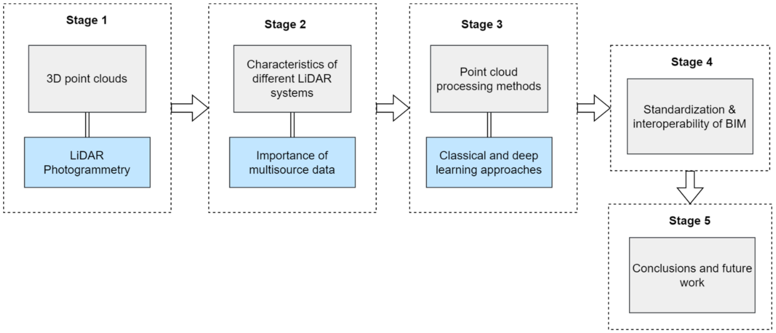
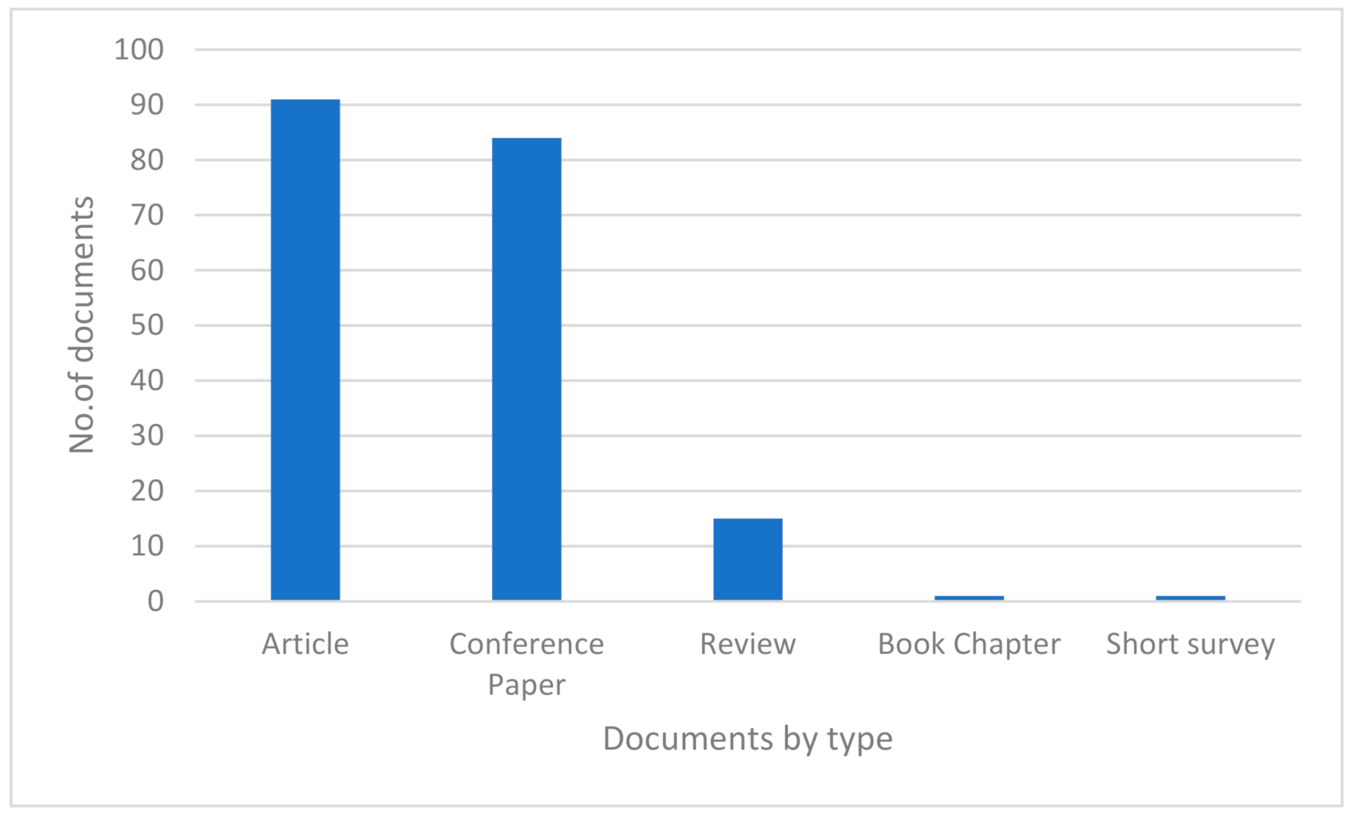
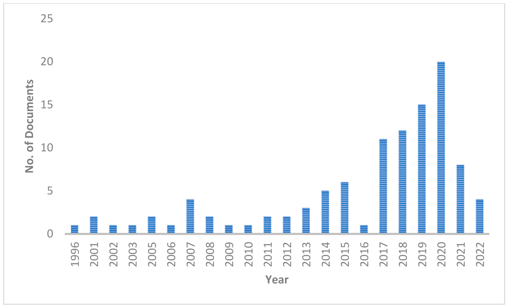
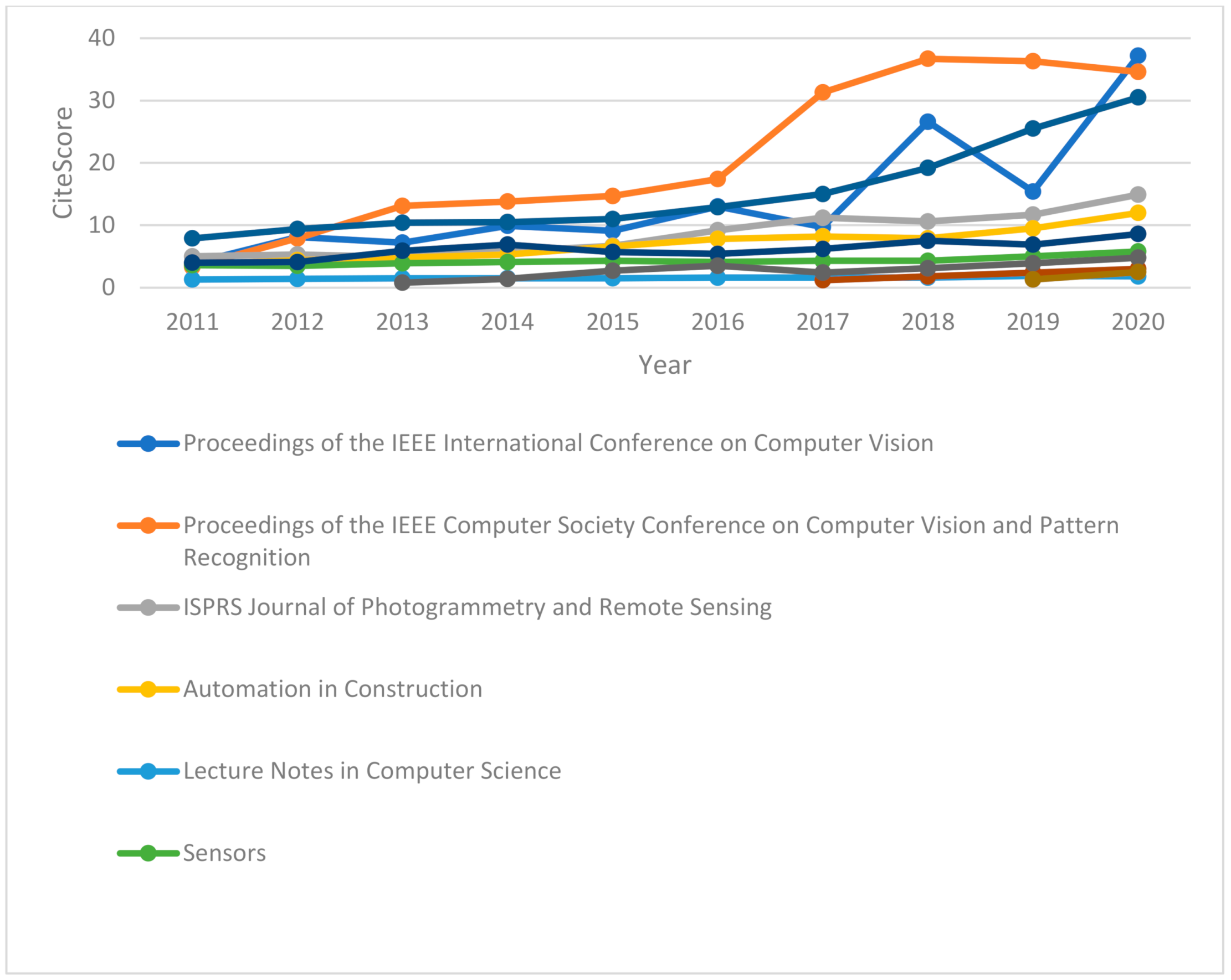
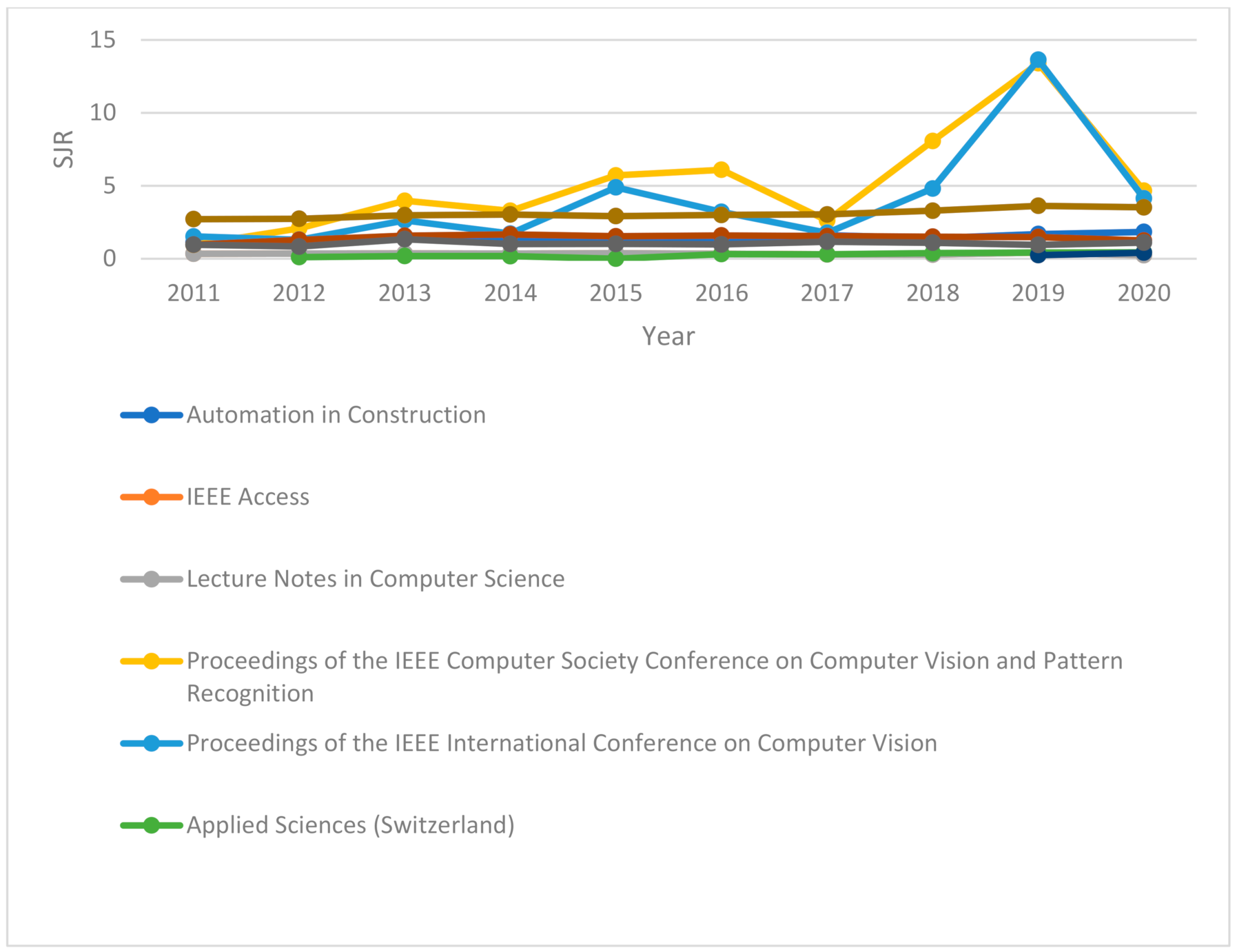
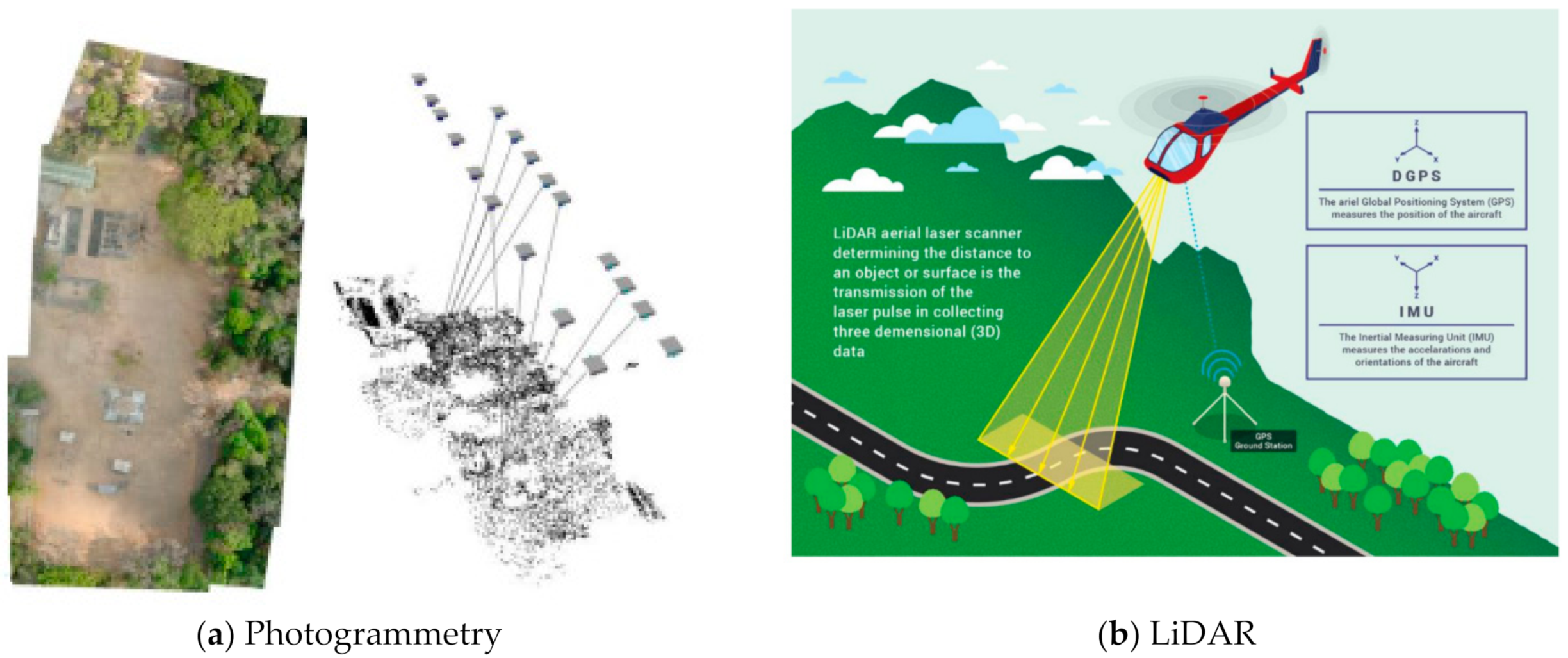
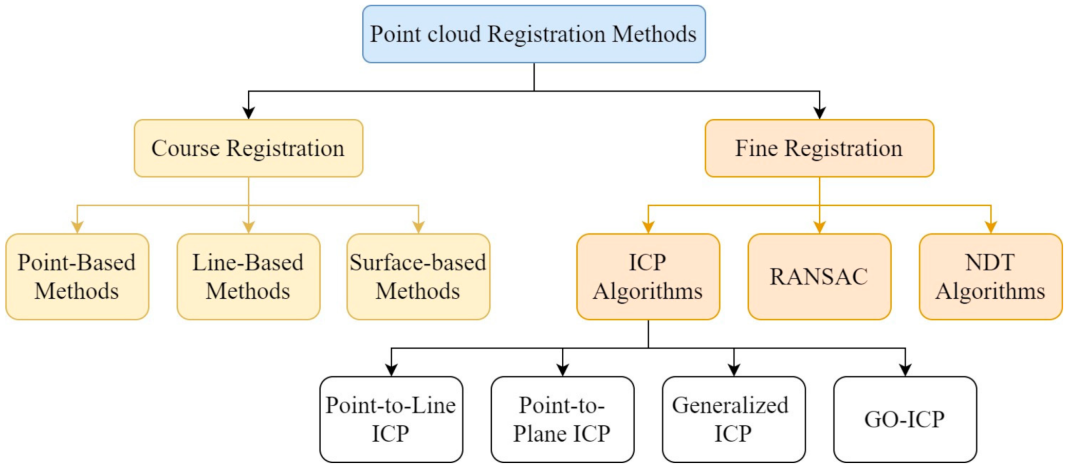
Figure 7.
Taxonomy of classical registration methods for 3D point clouds.

Table 1.
Literature search keywords.
| Aspect | Keywords |
|---|---|
| BIM | “Scan to BIM”, “BIM”, “building information modelling” |
| Point-cloud processing | “automatic registration”, “sampling”, “point clouds”, “LiDAR”, “semantic segmentation”, “photogrammetry”, “deep learning”, “remote sensing” |
| Standards of BIM | “interoperability”, “open standards”, “IFC” |
Table 2.
Comparison of photogrammetry and LiDAR.
| Photogrammetry | LiDAR | |
|---|---|---|
| Sensor type | Passive sensor | Active sensor |
| Cost | Low | High |
| Point density | High | Medium |
| Automation level | High | Medium |
| Portability | High | Medium |
| Processing time | Low | High |
| Range | Medium | High |
| Usage in low-lit conditions | Low | High |
| Time flight | More flight time required | Less time flight required |
| Power consumption | Low | High |
Table 3.
Comparison of LiDAR systems on different platforms.
| LiDAR | Terrestrial LiDAR | MLS | ALS |
|---|---|---|---|
| Point density | Dense (>100 pt/m2) | Dense (>100 pt/m2) | Up to 50 pt/m2 |
| Scanning range | Point shape | Stripe shape | Surface shape |
| Accuracy | High accuracy (mm level) | High accuracy (cm level) | High accuracy (<15 cm) |
| Scanning perspective | Side view | Side view | Top view |
| Sensors | Laser scanner | GNSS, IMU, laser scanner | GNSS, IMU, laser scanner |
| Advantages | Provides the highest level of detail | Provides faster data, reduces acquisition time | Suitable for large area |
| Disadvantages | Not suitable for large infrastructure | Absolute accuracy is low because the satellite signals are blocked by buildings | Expensive for small project sites |
| Applications | Small area 3D reconstruction | HD mapping, urban monitoring, road mapping | Terrain mapping, vegetation monitoring, power line detection, bathymetric applications in shallow water |
Table 4.
Point-cloud down-sampling method.
| Down-Sampling Method | Test Platforms |
|---|---|
| Adaptive down-sampling | ALS, TLS, MLS |
| Octree-based down-sampling | ALS, TLS, MLS |
| OptD down-sampling | ALS, TLS, MLS |
| NSS | Mesh models |
| DNSS | Mesh models |
| SpDF | Challenging datasets for point-cloud registration algorithm [66] |
Table 5.
Deep-learning registration methods.
| Method | Year | Architecture | Testing Benchmarks | Applications |
|---|---|---|---|---|
| PPFNet | 2018 | PointNet | 3DMatch [105] | Indoor |
| PPF Foldnet | 2018 | PointNet | 3DMatch [105] | Indoor |
| PointNetLK | 2019 | PointNet | ModelNet40 [106] | Indoor |
| PCRNet | 2019 | PointNet | ModelNet40 [106] | Indoor |
| 3D FeatNet | 2018 | Siamese CNN | KITTI [107], ETH [66], OxfordRobot Car [108] | Outdoor |
| DCP | 2019 | DGCNN | ModelNet40 [106] | Indoor |
| Deep VCP | 2019 | CNN | KITTI [107], Apollo-SouthBay [109] | Outdoor |
| FCGF | 2019 | ResUNet | KITTI [107], 3DMatch [105] | Indoor and outdoor |
| AlignNet-3D | 2019 | CanonicalNet, MLP | ModelNet40 [106], KITTI [107] | Outdoor |
| D3 FeatNet | 2020 | KPCONV | KITTI [107], 3DMatch [105], ETH [66] | Indoor and outdoor |
| DeepGMR | 2020 | PointNet | ModelNet40 [106], Augmented ICL-NUIM [110,111] | Indoor |
| PREDATOR | 2020 | GNN | 3DMatch [105], DLoMatch, ModelNet40 [106] | Indoor |
| Deep global registration | 2020 | 6DConv | 3DMatch [105], Augmented ICL-NUIM [110,111], Indoor LiDAR RGB-D [112], Stanford RGB-D, KITTI [107] | Indoor and outdoor |
| RGM | 2021 | RGM | ModelNet40 [106] | Indoor |
| PointDSC | 2021 | SC-NONLOCAL, NSM | 3DMatch [105], KITTI [107], Augmented ICL-NUIM [110,111] | Indoor and outdoor |
Table 9.
BIM 1SO 19650 standards (information retrieved from [189]).
Table 9.
BIM 1SO 19650 standards (information retrieved from [189]).
| IS0 19650 Standards | Description |
|---|---|
| BS EN ISO 19650-1 | Information management using building information modelling: Concepts and principles |
| BS EN ISO 19650-2 | Information management using building information modelling: Delivery phase of the assets. |
| BS EN ISO 19650-3 | Information management using building information modelling: Operational phase of the assets |
| BS EN ISO 19650-5 | Information management using building information modelling: Security-minded approach to information management |
Table 10.
Summary of open standards.
| Open Standards | Body | User | Focus |
|---|---|---|---|
| IFC | buildingSMART | AEC, BIM | Exchange of data |
| MVD | buildingSMART | AEC, BIM | Specifies which information to be shared |
| gbXML | Green Building Studio | AEC, BIM, energy modelers | Exchange of data between building design and energy model analysis |
| LandXML | Open Geospatial Consortium (OGC) | BIM, surveying engineers | Represents civil engineering and survey measurement data |
| LandINFRA | Open Geospatial Consortium (OGC) | BIM, surveying engineers | Defines land and civil engineering infrastructure |
| CityGML | Open Geospatial Consortium (OGC) | 3D city modelers | Represents and exchanges 3D city models |
Publisher’s Note: MDPI stays neutral with regard to jurisdictional claims in published maps and institutional affiliations. |
© 2022 by the authors. Licensee MDPI, Basel, Switzerland. This article is an open access article distributed under the terms and conditions of the Creative Commons Attribution (CC BY) license (https://creativecommons.org/licenses/by/4.0/).
Share and Cite
MDPI and ACS Style
Rashdi, R.; Martínez-Sánchez, J.; Arias, P.; Qiu, Z. Scanning Technologies to Building Information Modelling: A Review. Infrastructures 2022, 7, 49. https://doi.org/10.3390/infrastructures7040049
AMA Style
Rashdi R, Martínez-Sánchez J, Arias P, Qiu Z. Scanning Technologies to Building Information Modelling: A Review. Infrastructures. 2022; 7(4):49. https://doi.org/10.3390/infrastructures7040049
Chicago/Turabian StyleRashdi, Rabia, Joaquín Martínez-Sánchez, Pedro Arias, and Zhouyan Qiu. 2022. "Scanning Technologies to Building Information Modelling: A Review" Infrastructures 7, no. 4: 49. https://doi.org/10.3390/infrastructures7040049