GIS Integration of DInSAR Measurements, Geological Investigation and Historical Surveys for the Structural Monitoring of Buildings and Infrastructures: An Application to the Valco San Paolo Urban Area of Rome

Abstract

Structural health monitoring is a crucial issue in areas with different hazard sources, such as Italy. Among non-invasive monitoring techniques, remote sensing provides useful information in supporting the management process and safety evaluations, reducing the impact of disturbances on the functionality of construction systems. The ground displacement time-series based on the analysis of Differential Interferometric Synthetic Aperture Radar (DInSAR) measurements, as well as the information about the geology of the area and the geometry of the construction under monitoring, provides useful data for the built environment’s structural assessment. This paper focuses on the structural monitoring and damage assessment of constructions based on the GIS integration of DInSAR measurements, geological investigation, historical surveys and 3D modeling. The methodology is applied to the residential area of Valco San Paolo in the city of Rome (Italy). Once the geological interpretation has confirmed the results of the DInSAR measurements, a quick damage assessment that considers all the possible conditions of the pre-existing damage at the time zero of the monitoring is shown for a damaged manufact in the area. The presented results highlight how the strategy to correlate the DInSAR-monitored ground settlements with the damage scales allows potentially to monitor continuous construction systems.

1. Introduction

Existing systems of buildings and infrastructures (generally called constructions from herein) could reach or even overcome their service life, thus needing structural monitoring and assessment to be performed to verify their residual capacity. Among non-invasive structural monitoring techniques, remote sensing can provide useful information in supporting the management process and the safety evaluations, reducing the impact of disturbances on the building/infrastructure functionality. In particular, the ground displacement time-series based on the analysis of Differential Interferometric Synthetic Aperture Radar (DInSAR) data, combined with information about the geology of the area and the geometry of the structure under monitoring, can be of great help for the structural assessments.

Numerous applications of DInSAR satellite data for monitoring ground deformations induced by natural and/or anthropogenic processes—often resulting in structural damage and/or consistent human or economic losses—can be found in the literature. Among others, different studies assessed the ground instabilities induced by subsidence on single constructions (e.g., [1,2,3,4,5,6,7]) or extended urban areas (e.g., [8,9,10]). Similarly, different works studied the urban area of Rome, investigating the effects of vertical settlements related to subsidence or excavations on single buildings (e.g., [11,12,13,14,15]) or extended areas (e.g., [16,17,18,19]). An overview of the potential and limitations of the use of satellite radar interferometry for the assessment and monitoring of existing structures can be found in Talledo et al. [20], such as that the satellite data have been used to assess other external actions not related to subsidence (e.g., [21]).

Well-known building damage criteria used in geotechnical engineering practice [22,23,24,25,26,27,28] can be adopted for the diagnosis of structural damage induced by ground settlements generated, among others, by subsidence. Empirical methods (e.g., [7]), semi-empirical approaches (e.g., [29]) or analytical approaches (e.g., [30,31]) can be used to assess the damage.

Information derived from historical investigations of the monitored structure, visual inspections (e.g., photographic and dimensional surveys, damage assessment of the construction) and field investigations (e.g., geological assessment of the area) can be useful to implement an accurate structural monitoring system. On one side, the geometry of the building and the correspondence of the original drawing with the as-built details can be checked, providing useful data for both the 3D modeling and the technical knowledge of the structure. On the other side, the deformation response of the subsoil, either to structural loads or geological and environmental processes acting on it, depends on the geotechnical properties—mainly the deformability moduli—of the lithological units forming the subsoil. The recognition of the lithological units, the definition of their spatial distribution in the subsoil volume and the identification of the relevant geotechnical properties remain the main issues of an engineering–geological model of the subsoil of an area [32,33]. The aim of the geological model is to support the interpretation of the ground movements (e.g., vertical displacements as induced by subsidence) observed over wider areas interacting with the constructions at both large and detailed scale [18].

In this research scenario, this paper focuses on the structural monitoring of constructions affected by subsidence based on the GIS integration of DInSAR data, geological investigation, historical surveys and 3D modeling. The methodology presented in this paper has been, then, applied to the residential area of Valco San Paolo in the city of Rome (Italy). This area, included in the larger area of the Tiber River bend, is characterized by significant ground movements affecting relevant constructions, as observed by processing some datasets of COSMO-SkyMed (CSK) SAR images (collected in the 2011–2019 time frame) through the advanced multi-temporal DInSAR techniques.

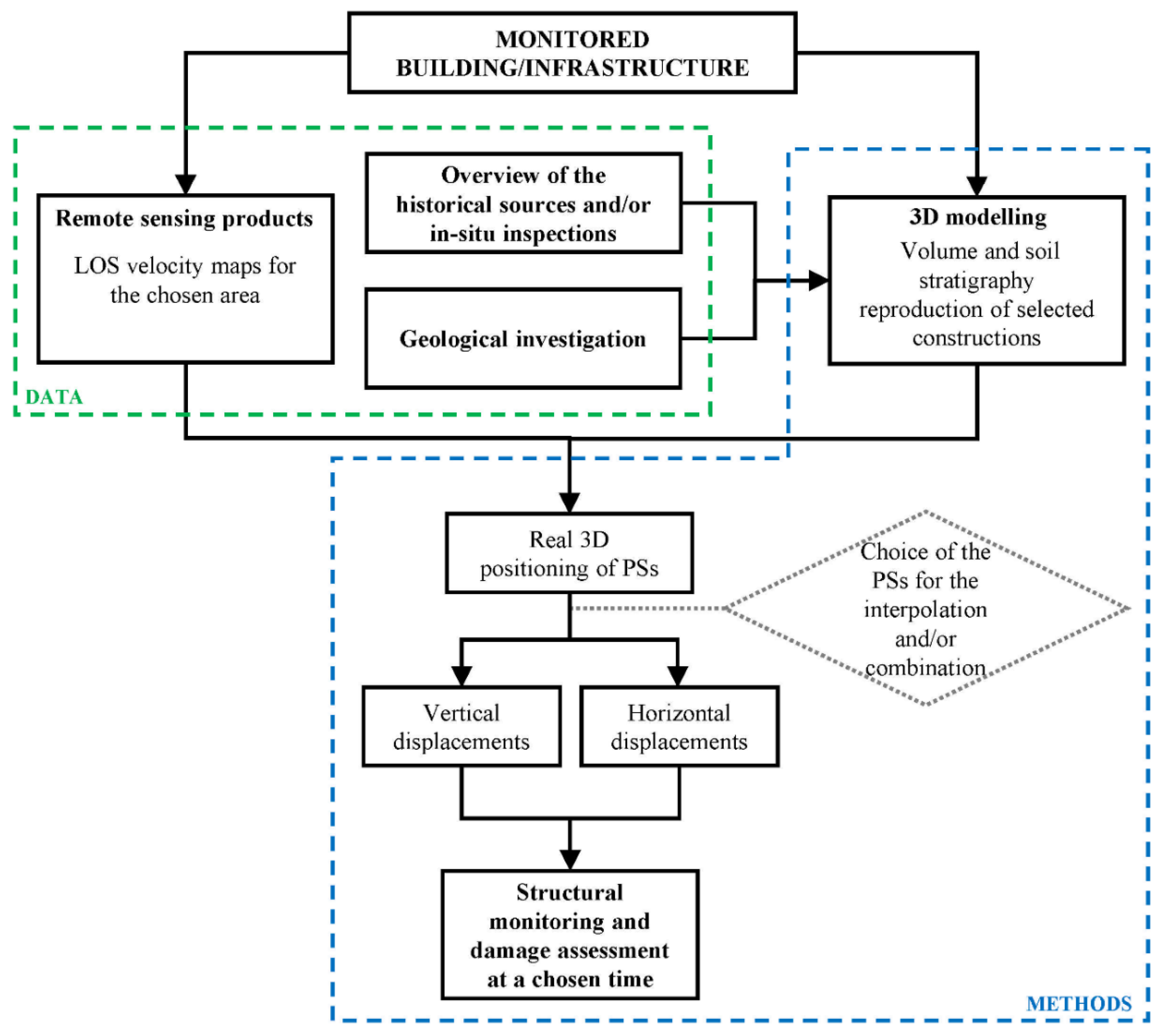
2. Materials and Methods

This section describes the methodology proposed for the structural monitoring of constructions, based on the GIS integration of DInSAR measurements, geological investigation, historical surveys and 3D modeling. The first step of the procedure shown in Figure 1 concerns the remote sensing products, achieved with the processing of the collected Synthetic Aperture Radar (SAR) images through the DInSAR analysis, which allows to retrieve velocity maps of the investigated area along the satellite Line of Sight (LOS, Section 2.1.1). Information from historical sources (such as technical drawings and cartographies), in situ surveys (Section 2.1.2) and geological investigations (Section 2.1.3) are exploited for the 3D modeling of the investigated construction. The precise volume of the structure is integrated in a 3D modeling software with the geological setting of the terrain below the construction (Section 2.2.1). Once the volume of the construction is defined, it is possible to implement a site-specific procedure for its structural monitoring (Section 2.2.2). First, the DInSAR-derived measurement points, referred to as persistent scatterers (PSs), are precisely located in the 3D space. Then, different strategies of interpolation of the velocity maps and combinations of the PSs can be used to define the vertical and horizontal (East−West) components of the LOS velocity vectors. Finally, the structural damage of the investigated construction is evaluated and ranked according to well-known damageability criteria (e.g., [28]).

2.1. Materials

2.1.1. Remote Sensing

Displacement measures for targets located on the ground surface can be obtained through the well-established Small BAseline Subset (SBAS) approach [34,35,36,37], in the framework of the existing multi-temporal DInSAR techniques. Deformation time series and mean velocity maps are derived for each pixel of the SAR image along the sensor LOS, i.e., the direction joining the satellite sensor with the target on the ground, with sub-centimetric accuracy. The technique is based on the exploitation of a large number of SAR images, acquired by satellite sensors over the investigated area, during a certain time period, which are properly selected to generate a multi-temporal sequence of differential interferograms, representing the phase differences between pairs of SAR images. Small temporal and spatial separations between the acquisition orbits (defined as temporal and perpendicular baselines) characterize the selected interferometric SAR data pairs, thus allowing to minimize the noise effects and maximize the spatial pixel density. As reported by Casu et al. [38] and Bonano et al. [39], the mean deformation velocity and the single displacement measurements are characterized by a precision of about 1–2 mm/year and 5–10 mm, respectively.

Radar images of the same geographical area from different perspectives, namely the ascending (ASC) and descending (DES) orbits of satellites, allow the generation of LOS ASC and DES deformation time series and velocity maps, which contribute to the reconstruction of the real ground deformation process. The two independent sets of deformation measurements are also characterized by a time lag between measures of the two datasets, due to the difference of their first acquisition dates (temporal reference of each single dataset).

The precision and accuracy of the PSs georeferencing is an important aspect. In the case of full resolution CSK SBAS-DInSAR processing, the precision of the PSs georeferencing can be assumed about 1–2 m, 2–3 m and 1–2 m in the North−South (N–S), East−West (E−W) and vertical (V) directions, respectively, corresponding to about one standard deviation. Further details can be found in Di Carlo et al. [15] and Talledo et al. [20].

The ASC and DES measurements can be combined to retrieve the actual direction of the displacement vector of each PS of the whole investigated area. The N–S component of the displacement vector is not effectively detectable due to the near polar orbits of the radar systems, with the ASC and DES LOS directions being nearly perpendicular to the N–S direction. Given that we know the LOS information of the same point in the two datasets and the LOS directional cosines in the two acquisition geometries, named n_E-W,i and n_V,i (with i = ASC or DES), the components of the displacement or mean velocity vectors (generically identified as X in Equation (1)) along the V and E–W directions can be evaluated through the following system of equations:

$$\{\begin{array}{c}{\mathrm{X}}_{\mathrm{LOS},\mathrm{ASC}}={\mathrm{X}}_{\mathrm{E}-\mathrm{W}}·{\mathrm{n}}_{\mathrm{E}-\mathrm{W},\mathrm{ASC}}+{\mathrm{X}}_{\mathrm{V}}·{\mathrm{n}}_{\mathrm{V},\mathrm{ASC}} \\ {\mathrm{X}}_{\mathrm{LOS},\mathrm{DES}}={\mathrm{X}}_{\mathrm{E}-\mathrm{W}}·{\mathrm{n}}_{\mathrm{E}-\mathrm{W},\mathrm{DES}}+{\mathrm{X}}_{\mathrm{V}}·{\mathrm{n}}_{\mathrm{V},\mathrm{DES}}\end{array}$$

(1)

It is worth highlighting that it is rather unusual to find a biunivocal spatial correspondence between points of the two ASC and DES datasets, especially for buildings. A spatial resampling, starting from ASC and DES PSs sufficiently near to be representative with a good approximation of the same reflective target, is thus usually required to decompose the measured displacement along the vertical and E–W directions [12,40]. Continuous LOS mean velocity maps for each dataset can be obtained and projected on a defined grid to compute the vectors of the mean interpolated LOS velocities V_LOS,ASC and V_LOS,DES in each vertex of the grid [15]. The V and E–W components (V_V and V_E-W, respectively) of each point of the above-mentioned grid can therefore be evaluated with Equation (1). The grid cell size, however, should not exceed the resolution of the satellite products (i.e., about 3 × 3 m² for CSK Stripmap data).

2.1.2. Historical Analysis and Field Surveys

Documental research is the first step to acquire a base technical knowledge of the monitored construction. By cross-checking the written and iconographic sources related to the original design and construction site projects of the construction, a base knowledge of both the geometry and the “hidden” building details of the structure can be achieved. Furthermore, in the preliminary analysis of the area, historical investigations can be also useful to detect—exploiting historical cartography—the original path of some elements of the infrastructures that nowadays are buried underground (e.g., the sewerage).

The data derived from the historical investigation can be confirmed via field surveys and photographic surveys. In particular, the geometry of the building and the correspondence of the original drawing with the as-built details can be checked providing useful data for both the 3D modeling and the technical knowledge of the structure. Field surveys, supported by the technical knowledge of the structure derived from the historical survey, can also provide base information about visible damage and decay phenomena.

2.1.3. Geological Investigation

Structures and infrastructures interact with significant volumes of subsoil, in numerous cases bigger than the portion directly beneath their foundations. In this portion of subsoil, the stress state is directly modified by the structural load and the corresponding deformative response of the subsoil is controlled by the geotechnical properties of the soil/rocks enveloped in it. This portion of the subsoil is conventionally named the “pressure bulb” according to the Boussinesq theory [41]. In addition to the delimited volume of the “pressure bulb”, geological and environmental processes eventually occurring in the subsoil should be considered in the investigation. It has been demonstrated by a number of case histories that these processes could cause deformations at a larger scale than the single building including the subsoil where the foundations are placed, thus consequently inducing additional displacements to the structures and infrastructures independently from their own load. This refers, for instance, to subsidence triggered by water withdrawal in deep aquifers [42,43] or subsidence due to secondary consolidation processes in normally consolidated soils [44]. The deformation response of the subsoil, either to the structural loads or to the geological and environmental processes acting on it, depends on the geotechnical properties—mainly deformability moduli—of the lithological units forming the subsoil. The recognition of the lithological units, the definition of their spatial distribution in the subsoil volume and the identification of the relevant geotechnical properties remain the main issues of an engineering−geological model of the subsoil of an area [32,33]. The aim of the engineering−geological model is to support the interpretation of the ground displacements observed over wider areas, also considering the portion of subsoil interacting with the foundations of structures and infrastructures located in it [18]. The reconstruction of the 3D geological setting of the investigated area aims also at generating engineering–geological models encompassing the essential geometries and properties of the significant volume of the subsoil, which are deemed relevant for the purpose and scale of a specific investigation.

2.2. Methods

2.2.1. 3D Modeling

The extended 3D modeling of the structures under monitoring and soil stratigraphy of the area supports the integration of the DInSAR measurements, geological investigation and historical surveys mentioned above. The 3D modeling of the volumes of the structures under monitoring use the combination of historical analysis and visual survey as input data. The geological investigation provides input data for the 3D reconstruction of the soil stratigraphy in terms of spatial distribution of different lithotypes.

The construction of the integrated 3D model features 3 steps: (i) 3D parametric modeling of the volume of the structures under monitoring; (ii) 3D geological modeling of the soil stratigraphy; (iii) combination of the model of the structure with the geological model in the 3D GIS environment, including the positioning of the PSs. It is worthy to notice that, via the integration of the soil stratigraphic units with the actual geometry of the structure, the foundations are “visually” linked to the lithotype on or through which they are built, thus assisting in the analysis of possible causes of displacement of the topographic surface and structures under monitoring.

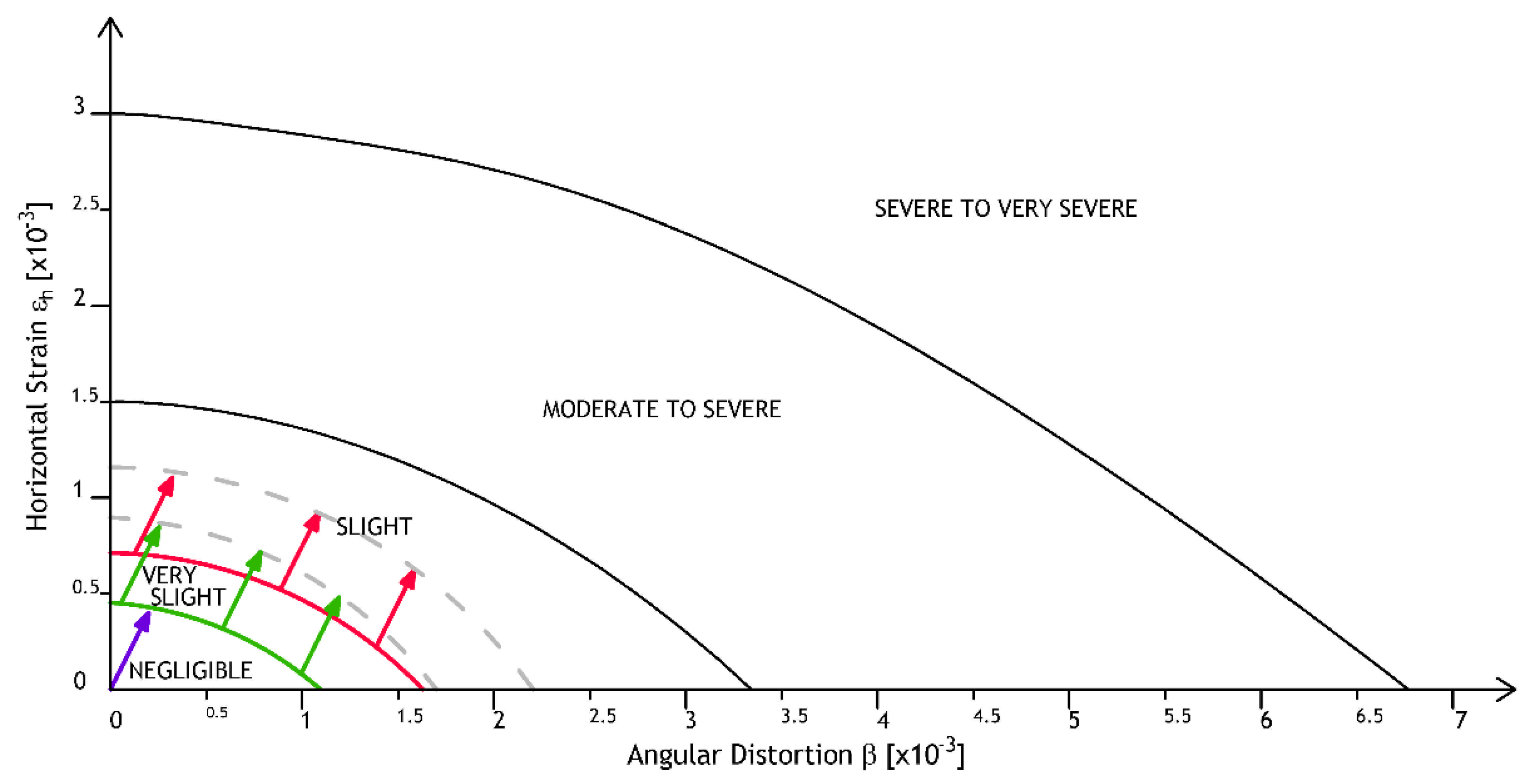
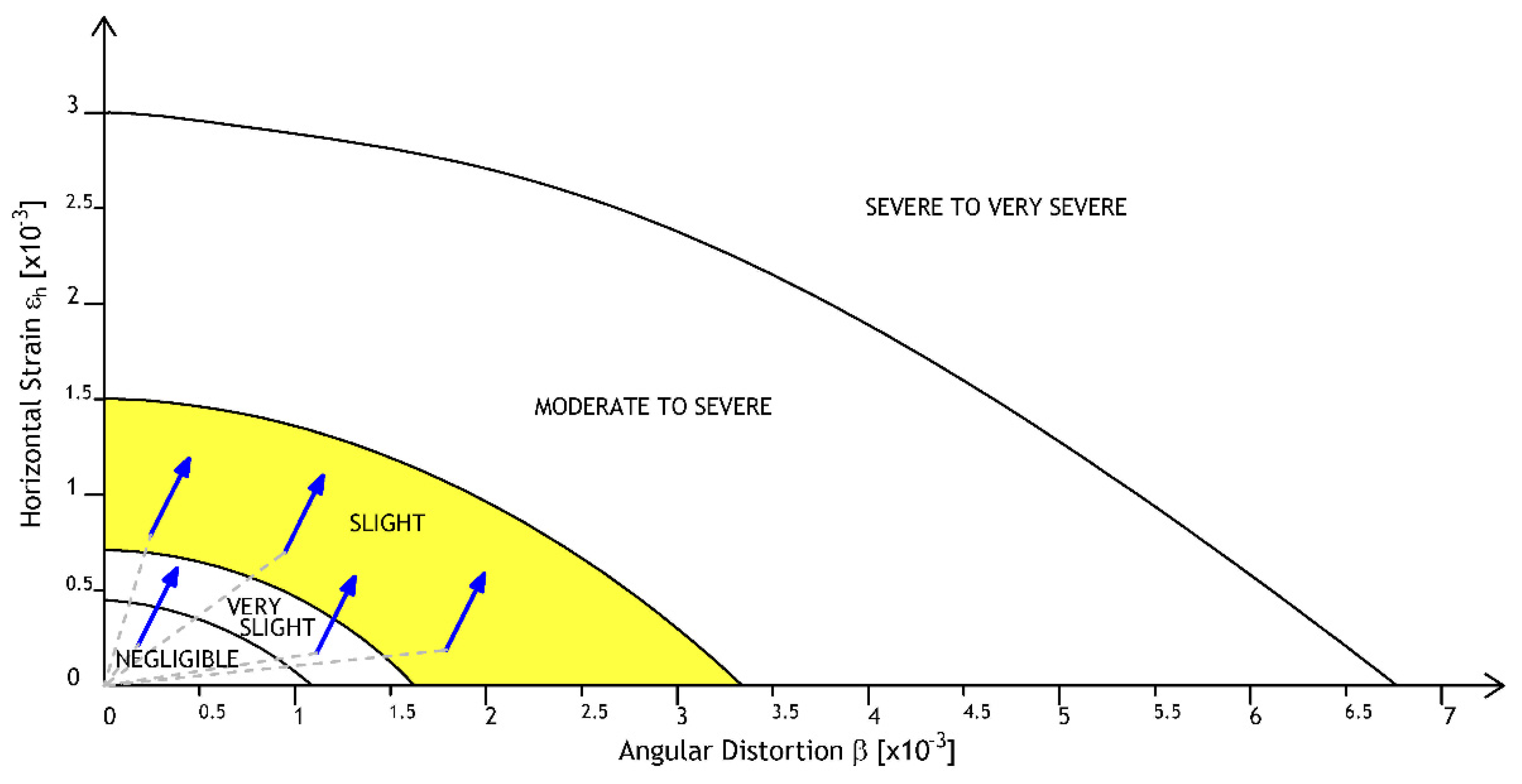
2.2.2. Structural Monitoring and Damage Assessment

In the framework of a preliminary structural damage assessment, the evaluation of the maximum displacements and the maximum differential settlements experienced by a structure is an asset to determine possible critical scenarios for the monitored construction. Deformations monitored through DInSAR techniques can be an input for a preliminary structural assessment of the condition of existing constructions. In this regard, it is fundamental to define the typology of external actions affecting a construction that can be potentially detected using DInSAR measurements. As demonstrated by the scientific literature, DInSAR measurements can be exploited to detect pseudo-static actions, as those related to ground deformations (e.g., subsidence, as in the case study presented in this work). The deformations induced on a construction by pseudo-static actions can be correlated with the damage observed on the structure via visual inspection of fractures on a set of building façades for different case studies. Cracking of building façades is generally assumed to be a consequence of angular distortion, expressed by the ratio of the differential settlement experienced by the foundation system and the distance between two points at the ground level. Skempton and MacDonald [22] summarized settlements and damage observations on mainly infilled steel and reinforced concrete framed structures. Meyerhof [23] treated the behavior of framed panels and loadbearing masonry walls separately. Then, Polshin and Tokar [24] discussed the allowable deformations and settlements for framed and load bearing structures and defined their limitations. Bjerrum [25] related the magnitude of the structure’s angular distortion to various types of damage, while Burland and Wroth [26] linked the onset of the visible cracking on the façades with a critical tensile strain. Burland et al. [27] proposed a five-level classification of damage based on the width of fractures on masonry buildings and correlated them to the maximum expected settlement/angular distortion. Boscarding and Cording [28] proposed a set of curves using the deep beam analysis to relate horizontal extension and angular distortion with the degree of building damage for brick bearing-wall structures.

Table 1. Summary of criteria for settlement and differential settlement of structures by sources from the literature, where L = length between panels and H = height (modified after Poulos et al. [45]).

Type of Structure	Type of Damage/Concern	Criterion	Limiting Value(s)
Framed buildings and reinforced load bearing walls	Structural damage	Angular distortion	1/150–1/250
	Cracking in walls and partitions	Angular distortion	1/500 (1/1000–1/1400) for end bays
	Visual appearance	Tilt	1/300
	Connection to services	Total settlement	50–75 mm (sands)
			75–135 mm (clays)
Tall buildings	Operation of lifts and elevators	Tilt after lift installation	1/1200–1/2000
Structures with unreinforced load bearing walls	Cracking by sagging	Deflection ratio	1/2500 (L/H = 1)
			1/1250 (L/H = 5)
	Cracking by hogging	Deflection ratio	1/5000 (L/H = 1)
			1/2500 (L/H = 5)

(synthesis by Poulos et al. [45]) summarizes different limiting values as a function of the type of structure and the type of damage/concern, as available in the literature. The main adopted parameter for the identification of the limiting values related to structural damage is the angular distortion previously described. For example, the limiting values of angular distortion to cause structural damage to columns and beams in framed buildings and to structures belonging to bridges with multiple spans are suggested as 1/150–1/250 and 1/250, respectively.

The methodology presented in this paper can be useful for a preliminary Structural Health Monitoring of buildings, enabling the assessment of the overall stability of an urbanized area. The damage classification can help establish a list of priorities of the most critical constructions for a better planning of more in-depth evaluations. Nevertheless, it should be clear that a complete structural assessment of an existing building can be performed only when the DInSAR measurements are supported by additional information, generally obtained from in situ inspections (e.g., for the definition of the material mechanical properties), to establish a structural model and to perform accurate structural checks. The proposed preliminary structural assessment can be repeated in different times, so it can be framed as a monitoring process [20].

3. Application to the Valco San Paolo Area in Rome

In this work, the residential area of Valco San Paolo in Rome has been selected as the sample case study area. Section 3.1 presents the interdisciplinary surveys conducted on the area. Section 3.2 explains the integrated 3D modeling procedure and the positioning of the PSs in the GIS environment. In Section 3.3, the structural monitoring and damage assessment of selected constructions are performed by analyzing the V and E–W components’ velocity maps of the area.

3.1. Analyses of the Area: SAR Data, Historical Sources and Geological Overview

In this section, the area is analyzed from the threefold point of view of the SAR overview of the area (presented in Section 3.1.1), the historical surveys and field surveys (presented in Section 3.1.2) and the geological overview of the area, with the identification of the stratigraphy of the soil (presented in Section 3.1.3).

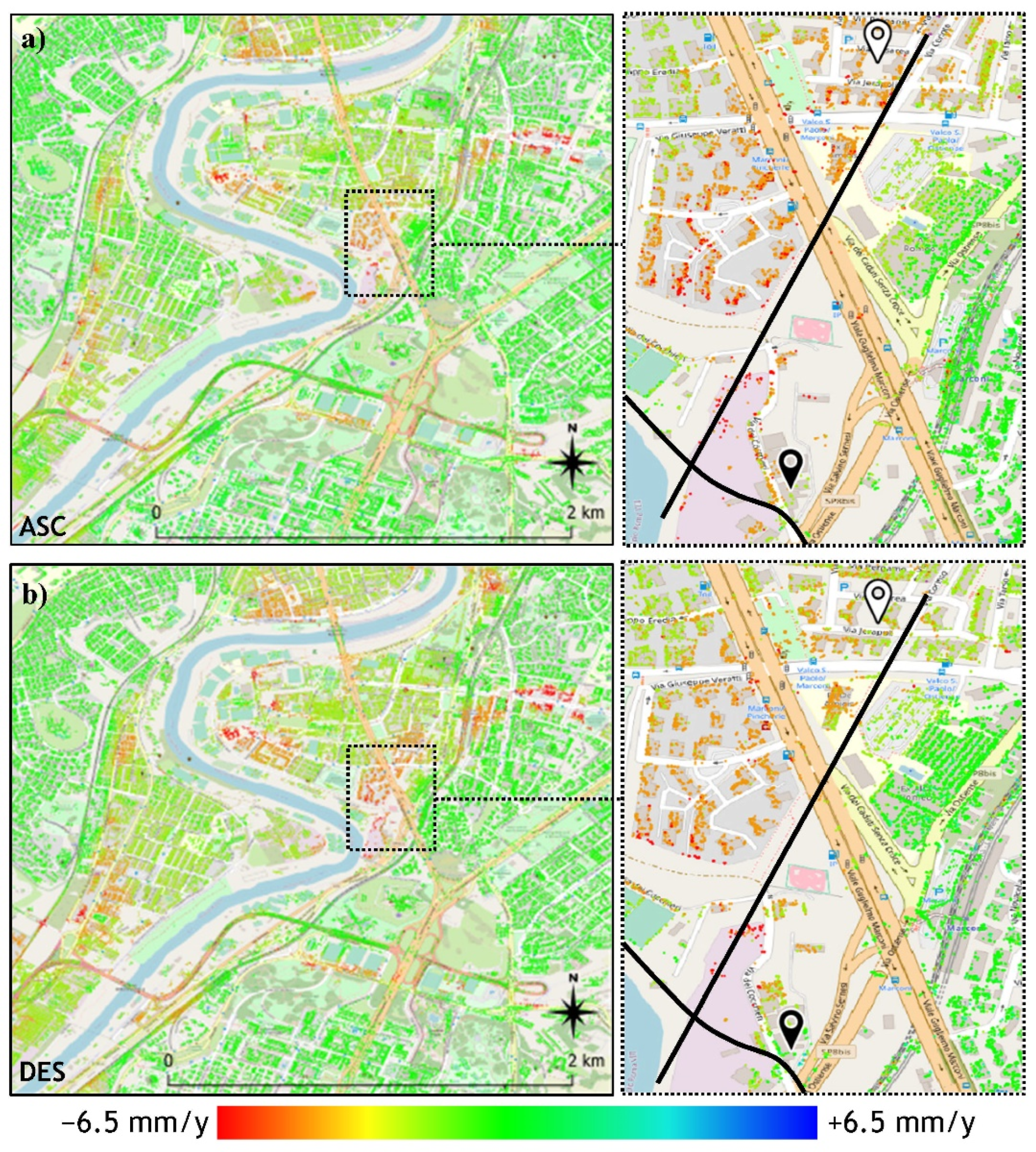
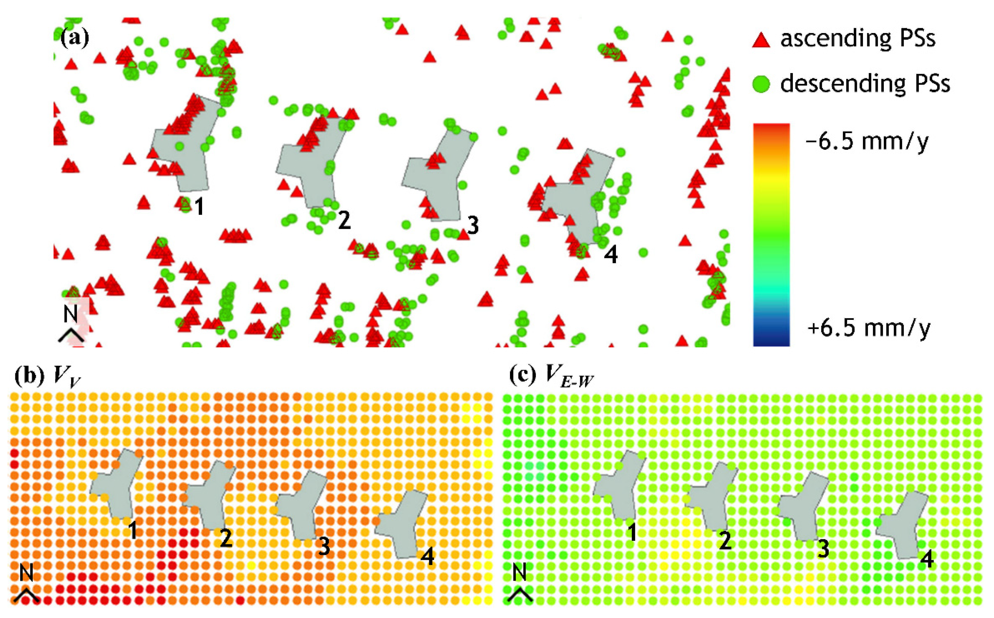
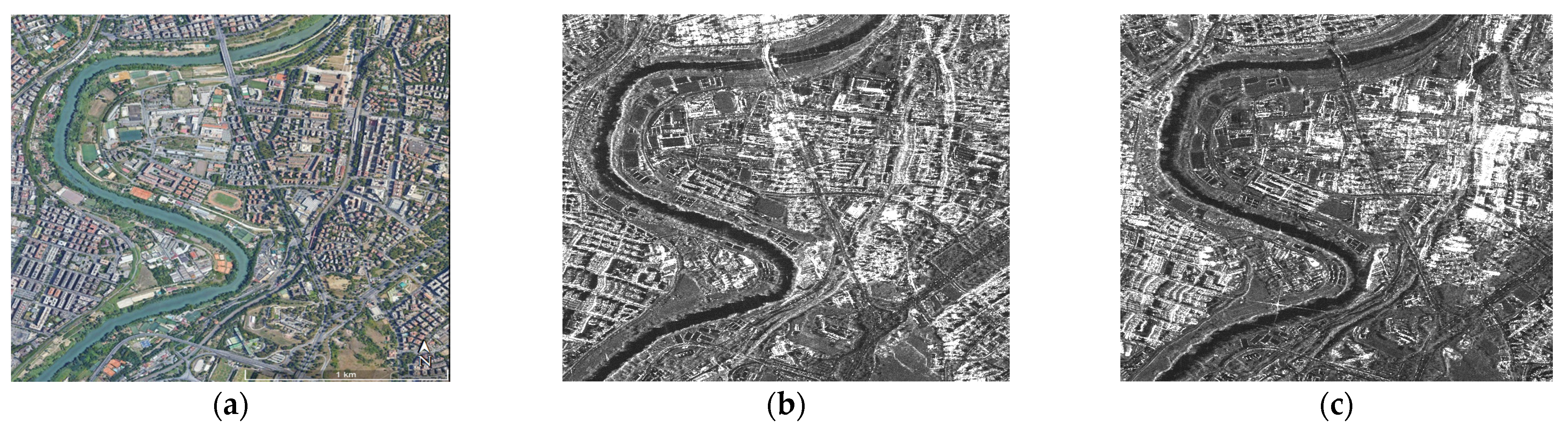
3.1.1. SAR Overview of the Area

The interferometric products used in this work have been obtained by applying the full resolution SBAS-DInSAR approach [36,39] to ASC (129 images collected between 23 March 2011 and 11 March 2019, average look angle ~34°, Beam-ID: H4-05) and DES (107 images between 29 July 2011 and 13 March 2019, average look angle ~29°, Beam-ID: H4-03) SAR images, obtained by the sensors of the Italian CSK constellation. The images are acquired through the standard Stripmap mode with HH polarization and a ground spatial resolution of about 3 m in both azimuth (along-track) and range (cross-track) directions. The full resolution deformation time series and corresponding LOS mean velocity measurements of each PS have been computed by using the 1-arcsec Shuttle Radar Topography Mission (SRTM) DEM of the study area, to remove the topographic phase component. The main parameters of the exploited datasets are summarized in

Table 2. Main parameters of the dataset.

Wavelength	~3.1 cm
Acquisition mode	Stripmap H-IMAGE
Spatial extension	~40 km × ~40 km
Spatial resolution of the interferometric data	~3 m × 3 m

.

A large overview of the area of interest is represented in Figure 2a, accompanied by two temporal multilook SAR images in ASC and DES acquisition orbit, respectively, in Figure 2b,c.

The LOS mean velocity maps are shown in Figure 3a,b for the ASC and DES orbits, respectively, expressed in cm/year and referring to the 2011–2019 time span. A zoomed-in view of the Valco San Paolo area and on the investigated manufacts is also shown on the right side of each figure, marked with the black dashed lines. In particular, the investigated constructions are indicated with benchmarks, white for the Torri Stellari complex of buildings and black for the Collector sewer point of disposal n. 7. Moreover, the left lower Collector sewer, part of the Marana di Grotta Perfetta hydraulic management, is marked with a continuous line. High values of the LOS mean velocity can be observed in the area included into the two dashed rectangles reported in Figure 3a,b between the Marana di Grotta Perfetta watercourse and the Collector sewer arm. The maximum LOS mean velocity values observed in the investigated areas are on the order of 1 cm/year.

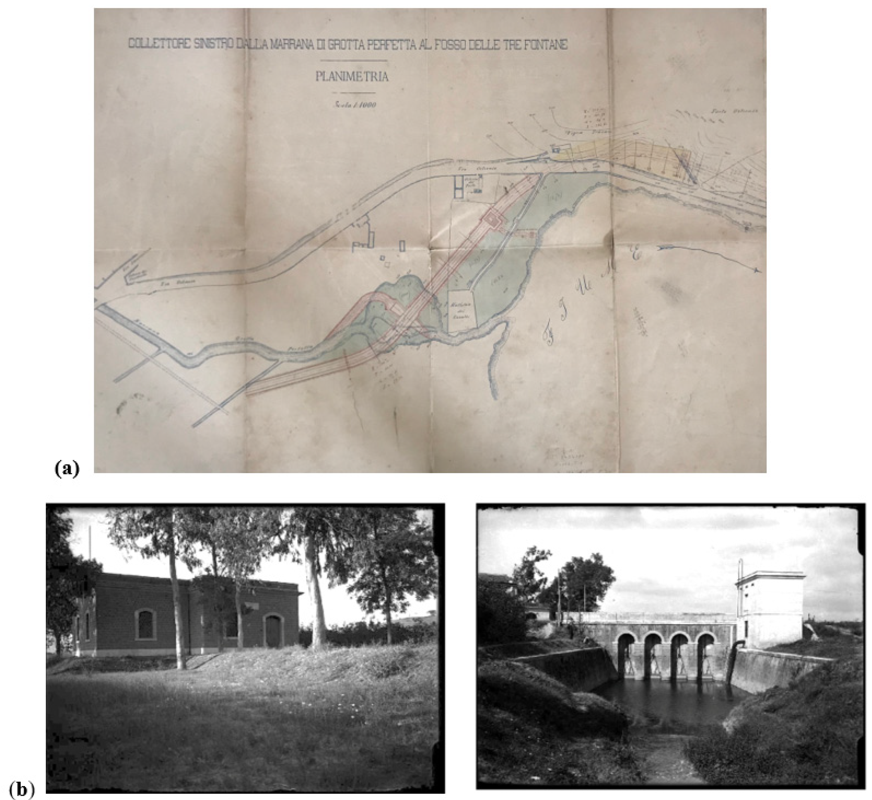
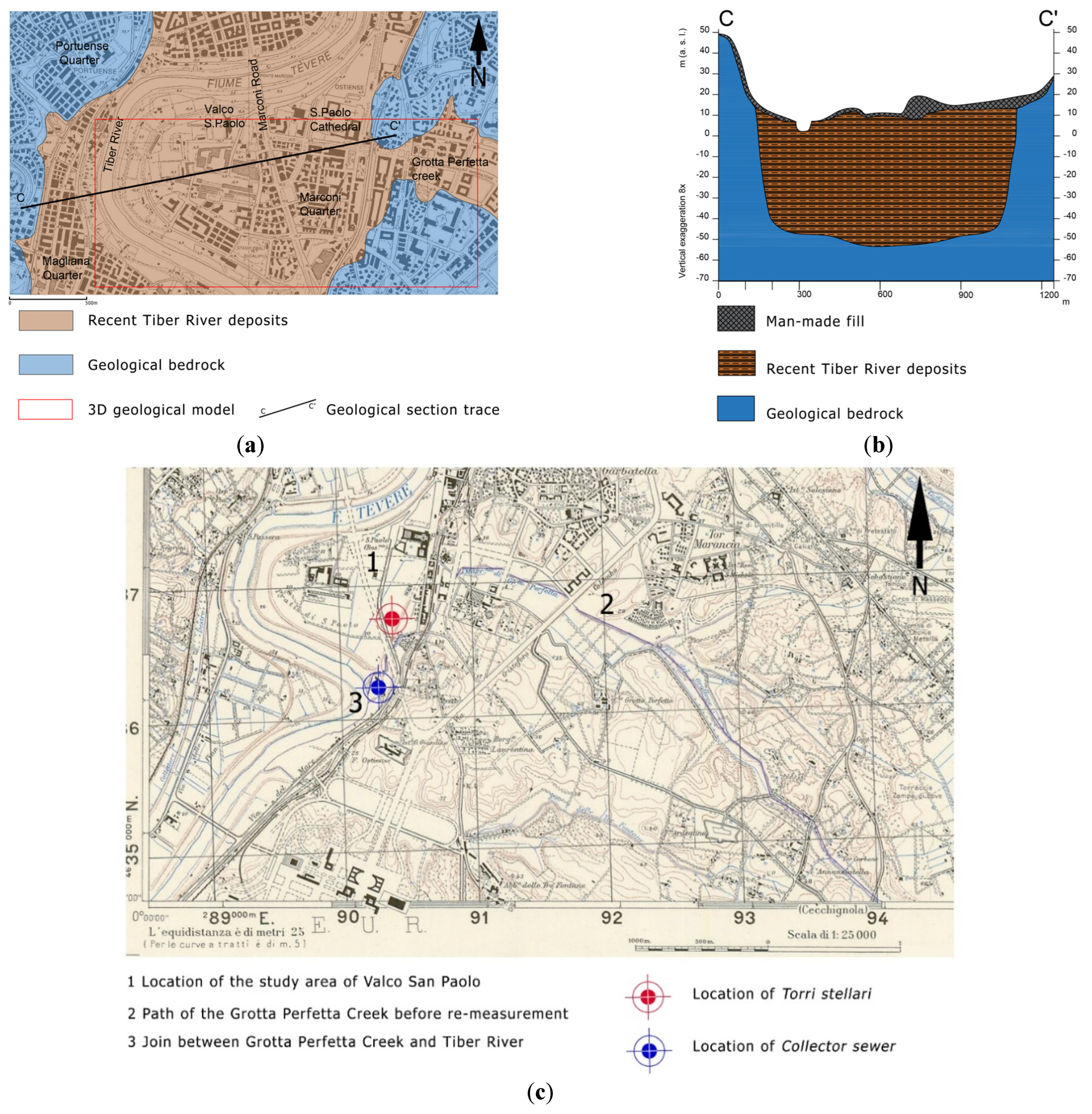
3.1.2. Historical Overview of the Area and Field Surveys

The Valco San Paolo area features the presence of 19th and 20th century heritage constructions: the hydraulic infrastructure, built between the end of the 19th century and the beginning of the 20th century, for the Tiber River and the watercourse of the Marana di Grotta Perfetta management, together with the improvement of the city’s sewage system (research, 1925) and the INA-Casa housing quarter built between 1949 and 1952 [46]. The housing district is indeed characterized by four 8-floor tower buildings, which feature a star-shaped plan. The load-bearing structure of the four towers is a reinforced concrete frame with brick walls and hollow block slabs. Due to these building characteristics, the towers can be considered a representative model of the Italian construction trends in post-war years. Regarding the hydraulic infrastructure, as shown in the historical cartography (Figure 4a), the area is crossed by the left lower Collector sewer, the related point of disposal and the passage works. The Collector sewer is an underground tunnel of an ovoid shape (5 m × 7 m), constructed in masonry. Also existing in the area is the point of disposal n. 7, a one-story building in tuff masonry positioned above the tunnel. The Marana watercourse crosses the Collector sewer with four tunnels of 1.80 m in diameter, passing through a bridge with four masonry arches and a two-story square control turret (Figure 4b).

Both the buildings of the INA Casa housing quarter and the hydraulic infrastructure are well documented by archival sources concerning technical documents of the design and construction time.

In particular, the study of the Torri Stellari complex focused on the available original design drawings and documentation collected in the archive of the architect Mario De Renzi (1897–1967), who elaborated the general plan and the execution design of the tower n. 1 [15]. The collections of the Genio Civile of Rome Archive proved to be an essential source for the technical characterization and the location of the hydraulic infrastructure. The cross-check of the technical drawings and reports, as well as the historical cartographies and pictures, allowed the correct location of the works in the considered area and the characterization of the actual geometry of the structure under monitoring.

In both cases, the original design drawings provided the knowledge of the geometry, the loadbearing structure and the execution details of each construction. Dimensional and visual checks of the external volumes were performed on-site on the tower n. 1 and the point of disposal n. 7 building, together with a photographic survey.

3.1.3. Geological Overview of the Area

The geology of the metropolitan area of Rome is widely discussed in the scientific literature [47,48,49,50,51,52,53,54]. The geological history of the case study of the Roman area can be roughly summarized in four phases characterized by different environments:

1.

Sedimentation in the marine environment of a subsident basin, from Pliocene to lower Pleistocene;

2.

Filling of the basin by marine sedimentation with clayey deposits followed by sandy sedimentation, lower Pleistocene;

3.

Sin-glacial subaerial sedimentation with aggradational sedimentary cycles, linked to eustatic fluctuations and contemporary evolution of the Lazio volcanoes, middle Pleistocene;

4.

Final landscape modeling of the territory by erosive action of the Tiber River network during the last glacial period (named Wurm) followed by the filling of the main and secondary paleovalleys by alluvial sedimentation, from Late Pleistocene to Holocene.

The study area is bordered by a Tiber’s meander on its left bank to the west and the geological limit of the alluvial body with the right flank of the paleo-valley dug into pre-Holocene deposits, and a tributary of the Tiber River named Grotta Perfetta creek to the east (Figure 5a). The area is characterized by a large flat surface representing the alluvial plain of the Tiber River, slightly sloping toward the riverbed. In the schematic geological map of Figure 5a, the bedrock formations can be distinguished—including the marine, continental and volcanic formations deposited during the phases 1, 2 and 3 previously listed—from the recent alluvial deposits of the Tiber River, partially filling the valley excavated during the last glacial period (phase 4). In the geological section of Figure 5b, the geometrical relationships between the Tiber River alluvial body up to 50–60 m thick and the geological bedrock can be appreciated. At the east margin of the study area, the Grotta Perfetta creek is characterized by a small basin, whose main branches drain from the southern areas of the city of Rome (Tenuta di Tor Carbone, Tenuta di Grotta Perfetta) toward the Tiber River on the left bank (Figure 5c). From the XX century, the Grotta Perfetta creek, like other small hydrographic basins, is re-measured and conveyed inside a Collector sewer, which in turn leads into a deep collector that follows the path of the left bank of the Tiber River [55]. The recent alluvial deposits of the Grotta Perfetta valley are about 45–50 m thick. They are characterized by the presence of highly compressible organic soils, typical of a marshy depositional environment [56,57,58].

The recent and present alluvial deposits constitute a hydrogeological unit in the Hydrogeological Map of Rome [59]. They host an important confined aquifer located in the gravel layer at the base of the alluvial body [60] flowing from north to south along the path of the river. Some less important water circulation is located in the more permeable layers of the alluvial body.

The geological model of Valco San Paolo subsoil (the area in the red rectangle of Figure 5a of about 2.2 km²) has been reconstructed focusing on the details of the main recent alluvial body of the Tiber River. For this reason, the Grotta Perfetta creek and its filling have been considered as a part of the flank of the Tiber paleo-valley, as shown in the geological map of Figure 5a. Multi-source input data have been used: the Digital Terrain Model 5 × 5 (DTM) of Rome provided by Open Data Lazio service (www.dati.lazio.it, accessed on 2 May 2017), literature geological maps and cross-sections [51], and 31 stratigraphic logs of boreholes performed for several geognostic campaigns from 1989 to 2008. The boreholes reached different depths, from about 20 m to 70 m b.g.l. depth, and 6 out of 31 cross the alluvial body and reach the geological bedrock. All the input data were georeferenced to SR ED50/UTMzone33 EPSG:23033 and then reprojected in WGS 84 to uniform both geological and structural data.

The stratigraphic logs have been analyzed and interpreted with reference to the work of Bozzano et al. [48]. The following lithotypes (from the top to the bottom) of the recent alluvial body of the Tiber River have been distinguished:

• Lithotype R: anthropic fill material characterized by abundant, variously sized brick fragments and blocks of tuff embedded in a brown-green silty-sandy matrix;
• Lithotype A: mainly silty and secondly sandy deposits with traces of organic matter, identified with the historical alluvium;
• Lithotype B: brown to yellow (more rarely gray) colored, sandy and silty-sandy deposits;
• Lithotype C: gray clay and silty clay with a variable organic content that gives a local black color. Occasional up to 100 mm thick peat levels and rare sandy silt layers with gravel are also present;
• Lithotype D: alternating silty-sandy, sandy-silty, clayey-silty and clayey levels. Viewed together, this unit is gray in color;
• Lithotype G: predominantly limestone gravel in a gray, sandy-silty matrix;
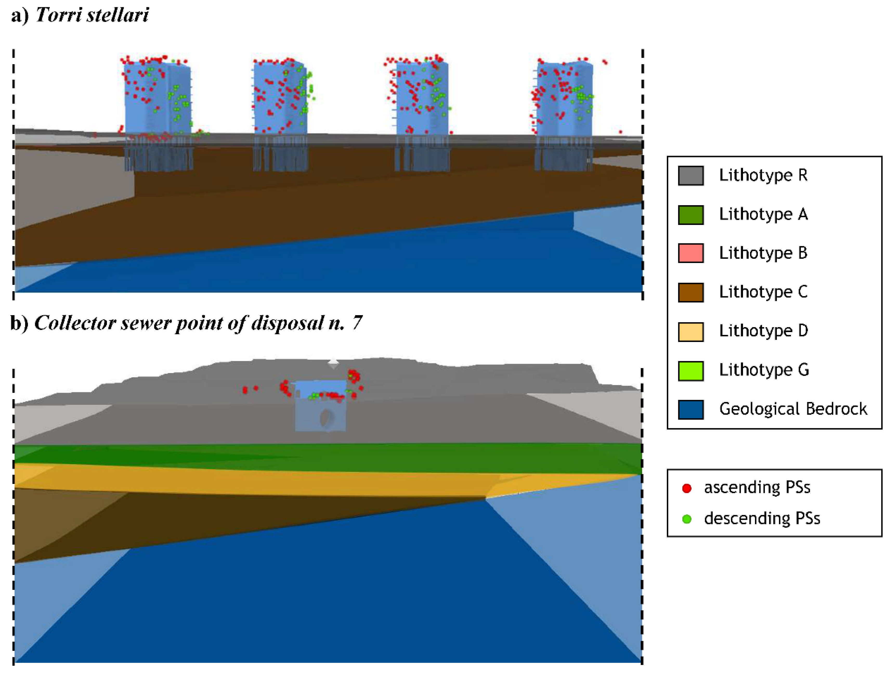
• Geological Bedrock: all the other pre-Holocene deposits that form the bottom and the flanks of the Tiber erosive paleovalley (Figure 5b). It is assumed that these over-consolidated sediments do not contribute to the settlement transmitted to the topographic surface and buildings.

The main part of the alluvial body is constituted by the lithotype C, which is a low-consistency, saturated, fine-grained soil characterized by the highest compressibility and lowest hydraulic conductivity with respect to the other lithotypes according to our geotechnical database. For this lithotype, oedometric tests allowed to estimate an oedometric modulus of about E = 6.7 ± 3.2 MPa. A compressibility progressively decreasing from lithotype C to lithotype A (mainly fine grained), followed by D, B and finally G (progressively shifting toward coarse grained material from loose to dense depending also on the depth below ground level), is inferred. Geological bedrock formations are assumed to be incompressible. Regarding the hydraulic conductivity, an increase from lithotypes C, to A, then D, B and finally G is expected. As already mentioned, lithotype G hosts an important confined aquifer of the hydrogeological unit named “recent and present alluvial deposits” in the Hydrogeological Map of Rome [59], while lithotypes B and D could host local and less important water circulations, thus shaping a multilayer aquifer. Mainly lithotype C and secondly A are considered as aquitards internal to this hydrogeological unit. The aquiclude of this multilayer aquifer is locally represented by the Marne Vaticane formation included in the bedrock (OC clays).

3.2. 3D Modeling

As explained in Section 2.2.1., the 3D modeling procedure features three steps following the selection of the input data derived from remote sensing, historical analysis, and geological investigation. The first step, the 3D modeling of the volume of the constructions, is explained in Section 3.2.1. The second step, the 3D geological modeling, is described in Section 3.2.2. The last step, the integration of the 3D model in the GIS environment, including the positioning of the PSs, is presented in Section 3.2.3.

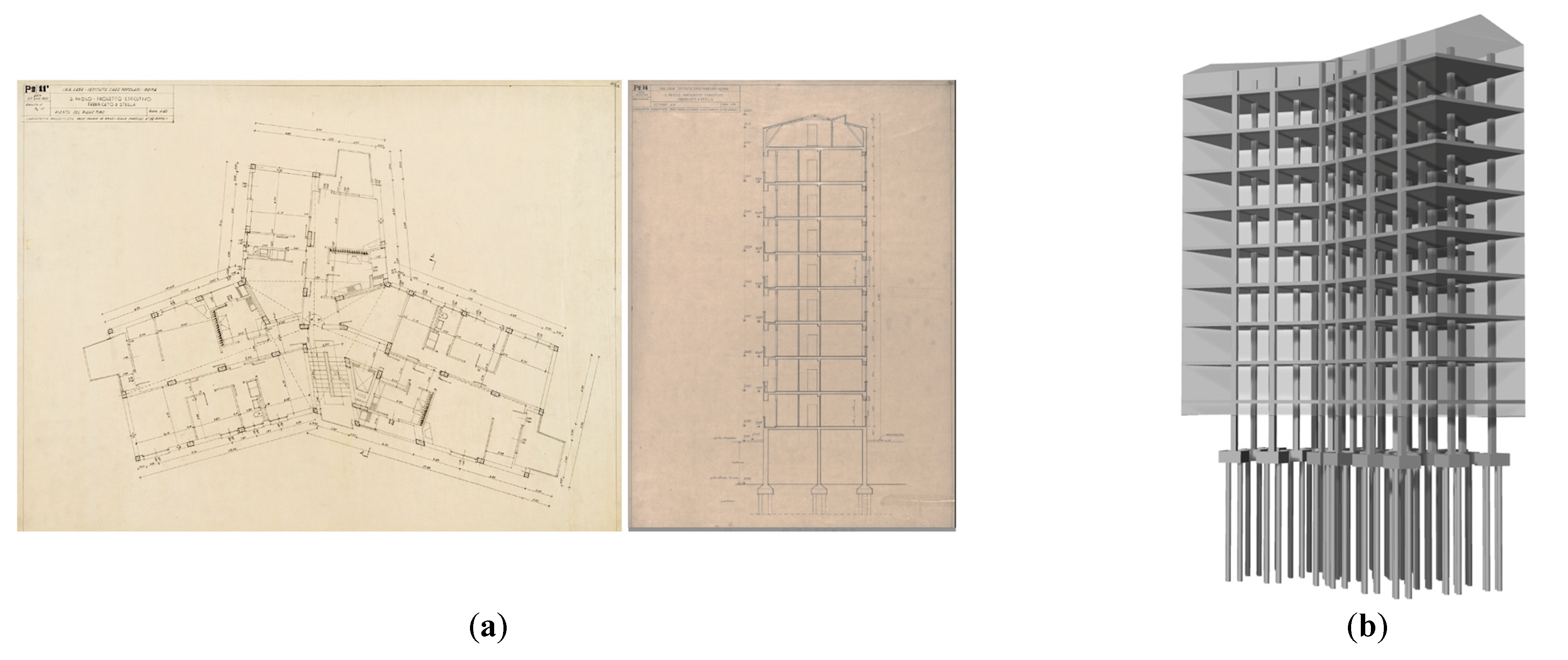
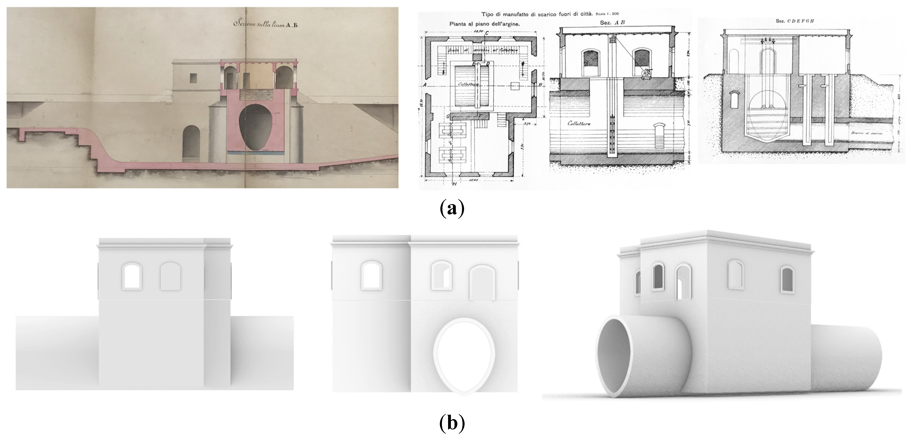
3.2.1. Architectural 3D Modeling

The architectural 3D modeling focuses on the Torri Stellari and on the building of the Collector sewer’s point of disposal n. 7. As described in detail in Di Carlo et al. [15], the 3D modeling process is based on historical documents. In particular, the geometrical data derived from the original drawings are used as input data for the 3D model reconstruction, exploiting parametric modeling and on-site surveys of specific building details. To integrate the building volumes in the geological 3D model, foundations and underground constructions were implemented in the architectural model.

As shown in Figure 6b, for the Torri Stellari, a schematic 3D model of the foundation system (plinths and piles) is derived from the historical sources (Figure 6a) and added to the building volume together with the elevation load-bearing structure (pillars and slabs).

For the building of the Collector sewer’s point of disposal n. 7, the 3D modeling focuses on both the reconstruction of the building external volume and the Collector sewer underground tunnel (Figure 7b). The data derived from the historical surveys—original cross-section drawings, plans, construction reports and pictures of the time (Figure 7a)—allow the modeling of the actual geometry of the underground tunnel.

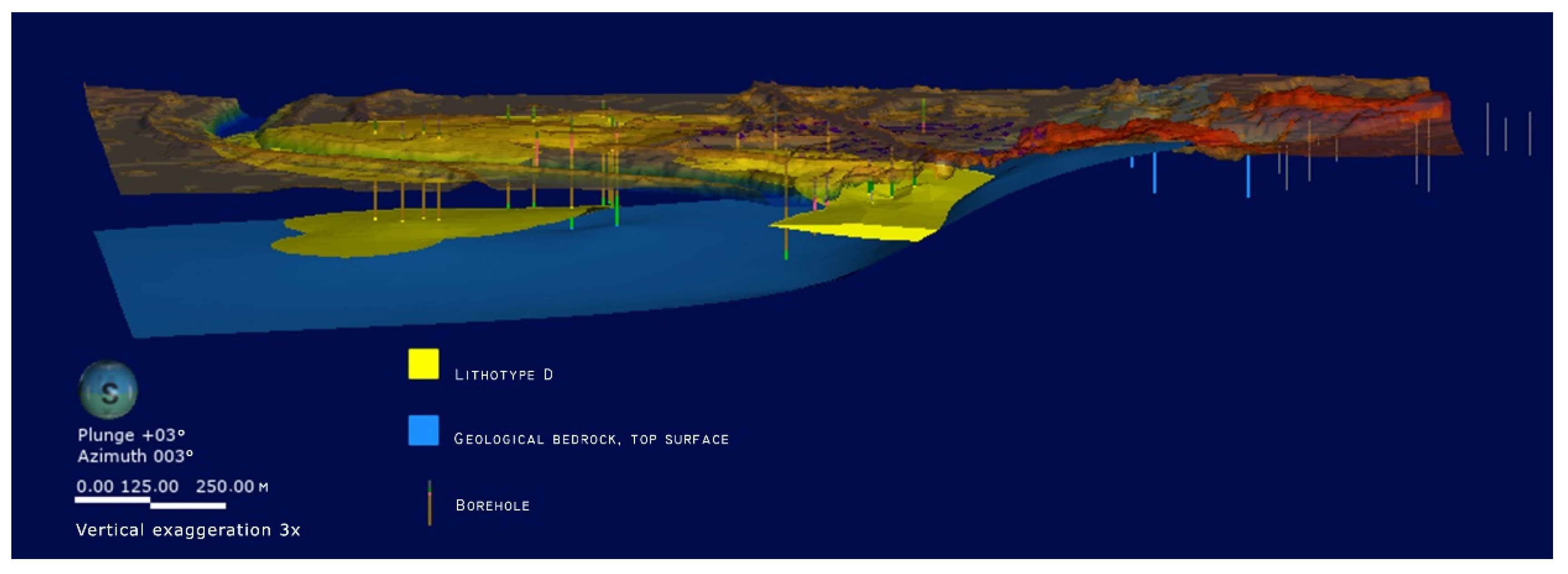
3.2.2. Geological 3D Modeling

Using the stratigraphic information mentioned in Section 3.1.3, a three-dimensional model of the subsurface has been reconstructed in the software package Leapfrog works 4.0 [61], as shown in Figure 8. The model is referred to the area delimited by the red box in Figure 5a. This model can be sectioned and exploded to better investigate the examined phenomena.

The 3D geological model shows the following main features:

• The basal surface of the alluvial body is the unconformity surface that sharply separates it from the formations constituting the bedrock represented by the blue color in the 3D model. The shape of this surface is concave upward, in the central part it is deeper (up to 70 m below ground level) and about horizontal, while in the eastern part is sloping toward the W-direction;
• In the lowest and deepest part, there is a bank about 10 m thick of lithotype G (predominantly limestone gravel in a gray, sandy-silty matrix). It is characterized by a flat horizontal top surface. Along the eastern flank of the buried paleovalley, this bank is lacking (Figure 8) as it is under the Torri Stellari aggregate and left lower Collector sewer areas (Figure 9);
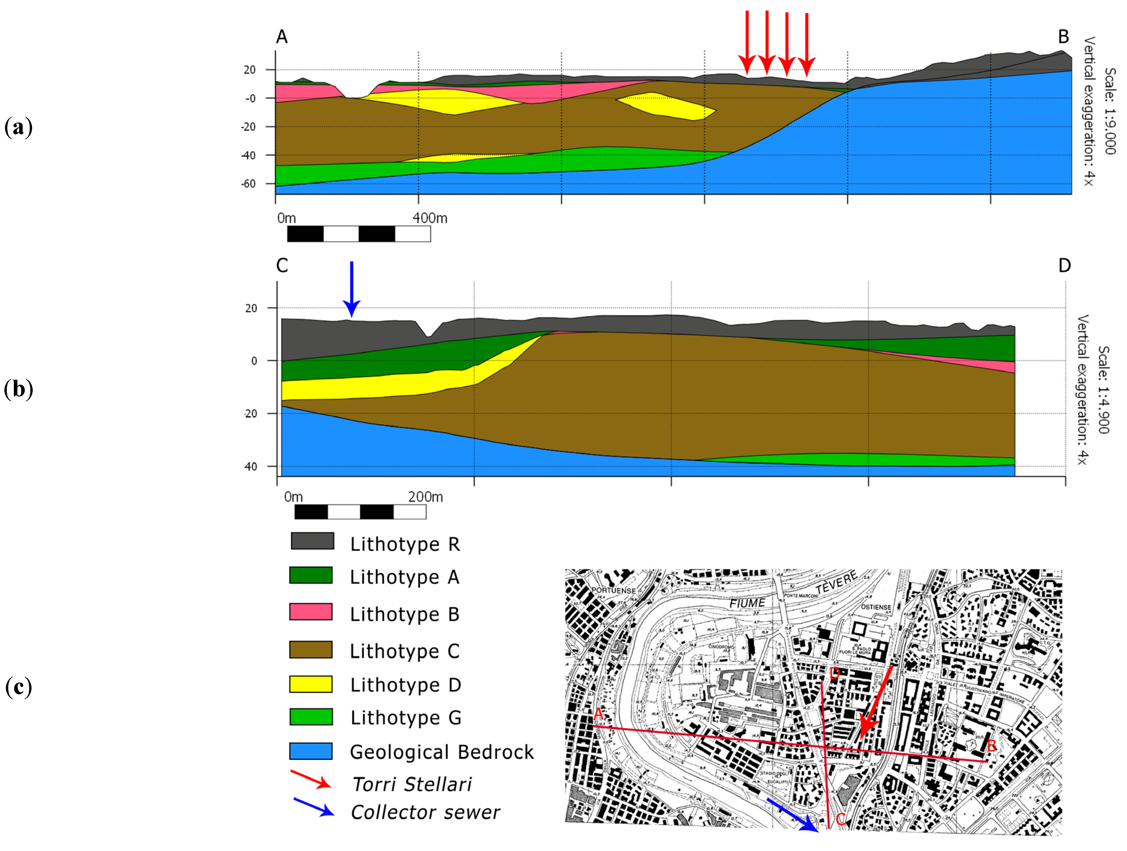
• Lithotype C—gray clay and silty clay with a variable organic content, a normally consolidated fine-grained soil characterized by the highest compressibility with respect to the other lithotypes, constitutes the main and huge part of the Tiber River alluvial body. In some parts of the model, it reaches thickness up to 50 m representing the only lithotype. This setting is observed in the central-eastern part of the area (Figure 9) where the Torri Stellari buildings are located. It can be observed here the direct contact of the lithotype C against the bedrock along the eastern flank of the Tiber River paleo-valley and the thickness of lithotype C decreasing of about 20 m from the western to eastern part, under this structural aggregate (Figure 9);
• In the main part of the alluvial body constituted by the lithotype C, there are some lenses of lithotype D (alternating silty-sandy, sandy-silty, clayey-silty and clayey levels). One lens of this lithotype is located in the subsoils of the confluence area of the Grotta di Perfetta creek in the Tiber River, where the left lower Collector sewer is located. In Figure 8, it can be observed that this area is near to the eastern flank of the Tiber paleo-valley. Here, the overall thickness of man-made fill and alluvial deposits overlying the bedrock is about 40 m, and the lithotype D lens is overlaying a thin layer of lithotype C over the bedrock and overlaid by lithotype A. It is possible that an aquifer is locally hosted in lithotype D, lens and lithotype A and C or the bedrock acting as aquitard/aquiclude;
• The upper part of the Tiber alluvial body is characterized by lithotype B (brown to yellow colored, sandy and silty-sand deposits) and lithotype A (mainly silty and secondly sandy deposits with traces of organic matter). The first one is lenticular shaped, and the main lens of this lithotype, about 10–15 thick, occupies the internal part of the Tiber meander. It has been tentatively interpreted as the sedimentary record of the lateral migration toward west of the Tiber meander;
• A layer of made fill covers the alluvial body with thickness ranging from few meters up to 15 m. In the area where the left lower Collector sewer is located, the thickness is the highest of our model (Figure 9).

Based on other similar experiences performed in other parts of the Tiber River alluvial valley in the urban area of Rome, the accuracy of our 3D geological reconstruction is of approximately a few meters in the x, y and z coordinates with respect to the location of boundaries between the lithotypes constituting the alluvial body. Furthermore, with regards to the spatial trend of thickness’ variations of the lithotypes along the sections and specifically in the subsoil under the selected areas, we are confident to have picked up the main ones.

3.2.3. 3D Modeling Integration

An integrated 3D model is composed of the union of the 3D models of the buildings’ external volumes, including the foundation structures, and the 3D geological model. The integration of the two 3D models is performed in the ArcGIS Pro [62] environment, exploiting a unique georeferenced system (using the World Geodetic System 1984 coordinate system, WGS 84) together with the positioning of the PSs. First, the different 3D layers of the geological model and the 3D volumes of the buildings are georeferenced by using their coordinates and merged in the GIS environment. Then, the PSs are positioned by their associated latitude and longitude. An empirical check of the relative PSs positioning to the buildings volumes is done. The integrated model allows to exploit the real positioning of the PSs on the actual building volumes and on the surrounding area. The error sources, compared to the plano-altimetric error of the in the positioning of the PSs, are also limited. In general, it can be stated that the accuracy level in the integrated model, derived mainly from the PSs coordinates accuracy, can be acceptable for the aims of the present methodology, which aims to maximize the information from the highest number of PSs and by using the deformations values with a step in the order of meters (e.g., inter-axis among columns).

The possibility to create a volume of the construction is important when the monitoring regards the single building. In this case, when satellite data with a great accuracy, as those derived from COSMO-SkyMed constellation, are available, it is possible to verify the position of the PSs on the actual building volumes, to distinguish those relative to the roof from those relative to the facades or to the ground. Then, in the geological 3D model, the stratigraphic logs of the soil−structure interaction can be visually checked. First of all, this information is important to understand if the final settlement profiles are those expected in relation to the soil typologies, to validate the reliability of the displacement results. Moreover, in the integrated model, it can be evaluated in which layer the structural foundations of the building are attested. This is very important for the final correlation of the estimated settlements under the monitored buildings, derived from the DInSAR measurements, with the geological characterization of the subsoil.

The integrated models, embedding the positioning of the PSs, are represented in Figure 10, with a focus on the Torri Stellari and on the building of the Collector sewer’s point of disposal n. 7.

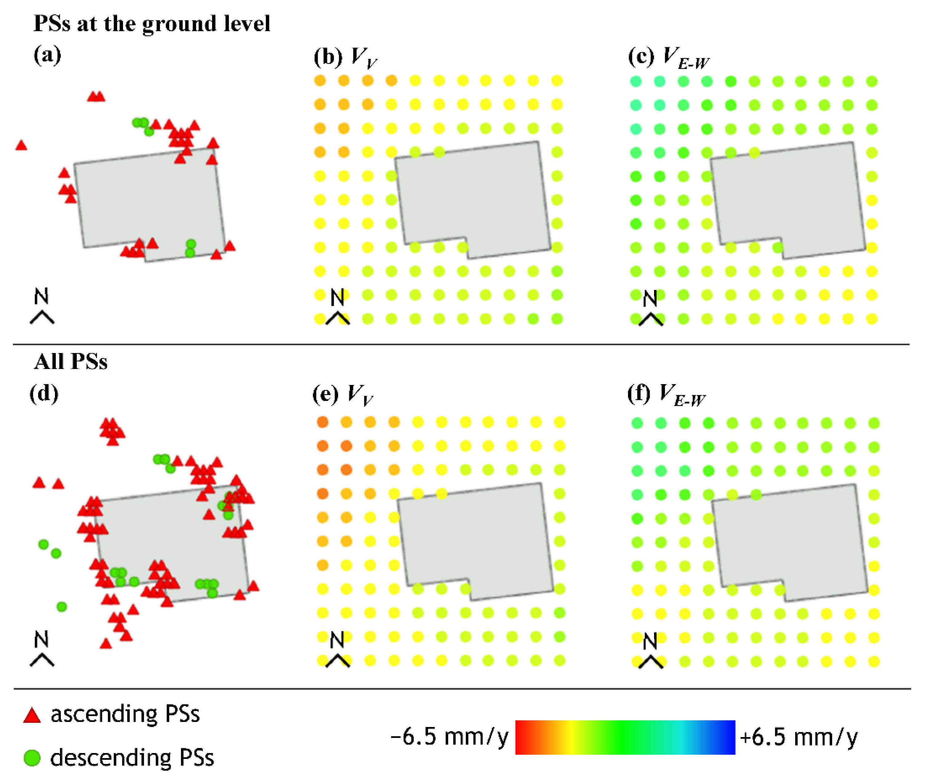
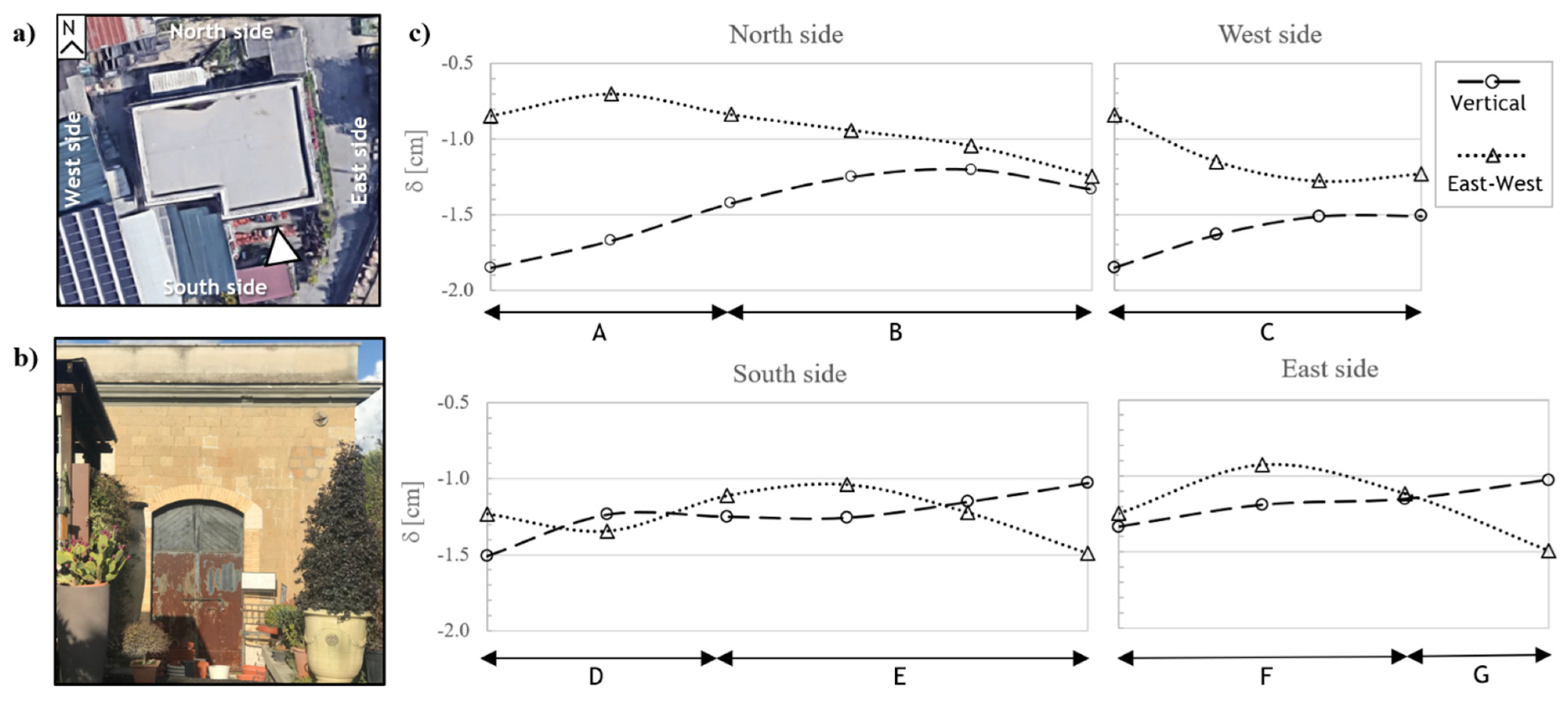
3.3. Structural Monitoring and Damage Assessment

A preliminary structural damage assessment is shown for the Torri Stellari complex and the Collector sewer point of disposal n. 7, both located in an area experiencing the highest ground deformations as detected by the DInSAR measurements.

Mean Deformation Velocity Maps Analysis

In this section, the vertical and E–W components of the mean displacement velocity measured through the DInSAR analysis on the ground surface are shown for the two case studies. The procedure for selecting the ground PSs, which has been repeated for the ASC and DES datasets, starts from observing their topography values. The topography values have been ordered in a descending manner, finding the maximum topography of the PSs related to the construction (excluding PSs with topography out of an admissible range, affected by processing errors). Then, 2 standard deviations of the altimetric error in positioning of the PSs (equal to 4 m) have been subtracted to that measure. The height of the roof level of the construction (H_roof) has been assumed to be the average of the measure of the maximum topography, and the “topography minus 4 m”. Since the real height of the construction (H) was known from historical documentation, the ground level at the base of the structure (H_ground) has been computed as H_ground = H_roof − H. The ground points have been selected with a confidence band around H_ground of ± 2 m, equal to the altimetric error in positioning of the PSs.

Then, a spatial resampling of both ASC and DES LOS velocity data has been implemented, using an Empirical Bayesian Kriging (EBK) interpolation method [63]. It is worth highlighting that this procedure is valid only under specific conditions of the disposition and trend of the selected points [15]. For example, when there is lack or a low number of PSs at the analyzed level, the use of interpolation techniques for the definition of velocity maps is not recommended.

Starting from the continuous interpolated maps, an auxiliary grid has been created to perform the arithmetic combination procedure explained in Section 2.1.1, for each grid vertex. The grid resolution has been set to 5 × 5 m², a value approximately equal to the distance between the columns, opportunely within the 3 × 3 m² resolution of the full-resolution COSMO-SkyMed products. For convention, upwards and east-directed displacements have positive values. Green zones are characterized by stable behavior. Figure 11b,c show the maps of the V_V and V_E-W in the area of the Torri Stellari buildings, obtained considering the PSs at the ground (Figure 11a), where the overlapping of some points with the building plan is considered caused by the PSs positioning error. Here, predominantly vertical settlements can be observed (Figure 11b), with negligible horizontal displacements (Figure 11c).

The same interpolation has been used for the Collector sewer point of disposal n. 7. Initially, the PSs located at the ground level, represented in Figure 12a from a top view (ASC and DES orbits, respectively represented with red triangles and green circles), have been considered. It is evident that the number of DES PSs is very low, and that their distribution around the manufact does not cover all the building sides. For this reason, to have a more consistent DES dataset, all the PSs around the manufact have been considered, without selecting them by height (Figure 12d, same symbol convention of Figure 12a). The mean velocity maps of V_V and V_E-W, for the Collector sewer point of disposal n. 7, have been derived starting from DInSAR measurements either using only ground PSs (Figure 12b,c) or all the PSs around the manufact (Figure 12e,f). Significant differences between the two maps are not observed, due to the low height of the construction. Then, the maps show the existence of downwards vertical settlements, and horizontal components comparable to the vertical ones. In this case, the cell size of the auxiliar grid has been set equal to 3 m, aiming at maximizing the number of measure points useful to build the settlement profile along the manufact’s sides, in order to implement the subsequent damage analysis presented in Section 2.2.2.

A procedure to check the reliability of the velocity maps obtained through the spatial interpolation process previously described can be found in Di Carlo et al. [15].

4. Discussions

The first step of the results analysis is the validation of the settlement buildings’ information, derived from the DInSAR measurements, with the geological characterization of the subsoil. It has been observed that the area of the Torri Stellari is characterized by predominantly vertical settlements (Figure 11b), with negligible horizontal displacements (Figure 11c). This can be attributed to a subsidence phenomenon ongoing from many years in the area [16,51]. It is worth noting that the Torri Stellari foundations pass through man-made fill and rest directly in lithotype C alluvium (see Figure 10a for comparison). A more detailed evaluation of the ground deformation has been conducted for the Collector sewer point of disposal n. 7, as damage compatible with settlements at the foundation depth has been observed on its facades. In fact, as it can be seen in Figure 10b, the manufact is located above lithotype R over placed on top of lateral heteropy between lithotype A and lithotype B (immediately outside of the area shown in Figure 8b and Figure 9b, and clearly shown in the 3D model in Figure 10), on top of about 8 m thickness of lithotype D lens.

Once the settlement profiles are compared with the geological characterization of the subsoil, the obtained maps are exploited to carry out engineering evaluations. In particular, by fixing a temporal span, they are used to derive base settlement profiles along the building’s sides in the considered direction. A damage correlation is done by associating the DInSAR-derived settlements or angular distortions experienced by each construction to literature classifications, such as those presented in Section 2.2.2. Field surveys are always useful to confirm the damage level found through the empirical correlations.

The damage−settlement correlation of the Torri Stellari buildings could not be performed because of recent renovation works that caused the loss of any existing trace of damage. Thus, such correlation is herein performed only for the Collector sewer point of disposal n. 7. To this end, the vertical and horizontal displacement profiles relative to each facade of the manufact (see Figure 13a) are represented in Figure 13c.

At the end of the monitoring period, the investigated building could show visible damage related to the deformation processes induced by one or more of the external actions. The damage assessment can be differently performed, depending on the knowledge of the condition of the monitored manufact at the time zero of the overall monitoring period. In general, two different cases can be distinguished:

1.

Lack of information on the damage status of the building at the beginning of the monitoring time;

2.

Available on-site survey at time zero (e.g., pictures or output data of a previous monitoring campaign).

Within the second case, two sub-conditions can be identified: (i) if the walls do not show visible damage at time zero, the actual damage can be evaluated neglecting the previous one and can be correlated to the cumulated displacements measured through the DInSAR observation time interval. This assumption should be carefully evaluated, because an ongoing tensional-deformational state that has not induced visible damage in the structural elements could be active, as better explained later; (ii) if a damage pattern is deductible at time zero, the actual damage represents its evolution.

An example of this approach for the damage assessment is here reported with an application to the southern external wall of the Collector sewer point of disposal n. 7, whose condition in December 2020 is reported in Figure 13b. According to Boscardin and Cording [28], the on-site survey led to classifying the wall condition as a slight damage because of the presence of cracks easily filled. Figure 13b represents the real condition of the case study building wall, for which no previous information is available at the starting time of the monitoring (case a). In this case (condition 1 of the previous list), the information about the damage at the end of the monitoring time (e.g., slight damage) is depicted in Figure 14 with a yellow-colored area. The blue arrows, instead, indicate the calculated horizontal strain/angular distortion couples of the selected wall, based on the displacement profiles shown in Figure 14. These arrows are shown in multiple positions because the precedent deformation history is not known. However, it can be argued that the ending point should be inside the yellow area.

Figure 15, instead, represents a conceptual application of the case 2, for which information at time zero is supposed to be available. The intensity of the arrow is the same as the precedent case. In this case, an initial damage status can be assigned to the building wall/side. Then, by summing up the calculated horizontal strain/angular distortion couple for the selected wall (herein proposed with different colored arrows based on the starting damage status), based on the displacement profiles, a new border surface can be identified at the end of the monitoring period (gray dashed curves). In some cases, the previous deformation can be considered negligible, while in other cases, an initial damage status should be assigned. It could be argued that it is not conservative to set the lower boundary curve of the identified damage status, as presented in the example of Figure 15. In fact, the authors suggest a criterion to solve this issue, based on the AeDES format sheets [64], accounting for the extension of the damage with respect to the structural element. The lower boundary curve of the damage status could be considered if its extension is between 0% and 33%, the median boundary curve (drawn with the same shape of the lower and upper boundary curves) if the extension is between 34% and 66%, and, finally, a curve just under the upper boundary curve if the extension is between 67% and 100%. In case of negligible damage, the starting point could be coincident with the origin of the axes of Figure 15, due to the low distance up to the achievement of the very slight damage, or the lower boundary curve of the very slight damage status could be conservatively considered.

Another issue is relative to the applicability of the different damage classifications available in literature, when dealing with the DInSAR data monitoring, taking into account the orientation of the monitored structural element. In fact, in the case of E–W (or with a small angle with respect to this direction) oriented elements, the classification proposed by Boscardin and Cording [28] is applicable, such as all classifications accounting for the horizontal strain. On the other hand, because of the lack of information about the N–S direction typical of the SAR acquisition systems, for N–S oriented elements, the use of literature classifications neglecting the horizontal strain is recommended.

In Figure 13c, the settlement profiles along the four sides of the building of the Collector sewer point of disposal n. 7 are represented, distinguishing the sagging and hogging portions with letters from A to G. With reference to the E–W oriented external walls, the values of the maximum angular distortion (β_max) and of the horizontal strain (ε_h) are reported in

Table 3. Maximum angular distortion β_max and horizontal strain ε_h of the east−west directed walls.

Settlement Profile Segment	βmax [−]	εh [−]
A	0.6 × 10−3	0.1 × 10−4
B	0.8 × 10−4	0.4 × 10−3
D	0.3 × 10−3	0.2 × 10−3
E	0.2 × 10−3	0.4 × 10−3

for the different segments A, B, D and E, in accordance with the sagging and hogging portions of the settlement profiles (Figure 13c).

For the N–S oriented walls, both the Polshin and Tokar [24] and the Meyerhof [23] criteria, specific for masonry walls structures, can be adopted.

A final focus regards the possible extendibility of the results for past analysis and future previsions. Retrospective analysis and/or future previsions—limited to a few years—could be performed by extending the results only if the data trend is well established in time. The extension could be done for the time series of the displacement components. However, with reference to the Collector sewer point of disposal n. 7, different trends were observed through the 8 years of monitoring. Therefore, an extension of the global trend for past analysis and/or future previsions cannot be accurate and may induce in error. A possible variation in the trend of the displacement time series does not enable us to make reliable assumptions about what happened before 2011 or after 2020, nor in the next future.

5. Conclusions

This paper focuses on the structural monitoring of constructions, based on the GIS integration of DInSAR measurements, geological investigation, historical surveys and 3D modeling. The methodology has been applied to the residential area of Valco San Paolo in the city of Rome (Italy). This area, included in the larger area of a Tiber River bend, is characterized by significant ground deformations as detected by DInSAR measurements collected between 2011 and 2019 by the SAR sensors of the COSMO-SkyMed constellation, and relevant buildings and infrastructures. The vertical component of the DInSAR mean deformation velocity maps obtained for the investigated manufacts highlight an overall higher settlement of the Torri Stellari (3–4 mm/year) rather than the Collector (1–2 mm/year). Such a difference can be attributed to the different construction materials (i.e., reinforced concrete and masonry), the foundation topology (i.e., deep for the Torri Stellari and shallow for the Collector) and the age of the manufacts (the Torri Stellari were built between 1949 and 1952, while the Collector was built in the first ten years of the 1900s) that influence the consolidation stage of the subsoil directly beneath the constructions. It is indeed expected that the Collector is in a more advanced state of consolidation than the Torri Stellari, thus justifying the minor rate of vertical settlement. The qualitative comparison between the DInSAR vertical velocity maps and the 3D engineering–geological model highlights also a possible correlation between ground settlements and litho-stratigraphic setting. As for the Torri Stellari, they manifest a heterogeneous vertical deformation with decreasing trend moving from west to east that remarks the variation of thickness from about 50 m to about 30 m of the lithotype C, where the building deep foundations are placed. Therefore, the compressibility of lithotype C and the ongoing consolidation process might be considered as the primary causes of settlement of these buildings. Although at smaller scale and magnitude, a similar trend of vertical settlements decreasing from west to east is experienced also by the Collector, which is founded on the lithotype R with thickness varying from about 10 m at west to about 15 m at east. In this case, the lithotype R and the proximal lithotype B are also in direct contact with the groundwater table emerging at about 200 m from the east bank of the Tiber River, whose level fluctuations might be an additional factor forcing the heterogeneous settlement of the hydraulic infrastructure. However, such considerations on the possible correlation between DInSAR-derived settlement and litho-stratigraphy are preliminary and need more detailed geological investigations beneath or in the surroundings of the analyzed manufacts.

Furthermore, a quick structural building damage assessment can be performed by applying the procedure proposed in this paper, depending on the knowledge of the condition of the monitored construction at the time zero of the monitoring period. The proposed methodology allows to provide a damage assessment in a short time, taking into account all the possible conditions of pre-existing damage at the time zero of the monitoring. Clearly, this framework performs better at medium−large scale, where the condition assessment of a system of buildings or infrastructures is more relevant. This procedure can be repeated for a select number of constructions (bridges, buildings, etc.) in the examined area, establishing a list of priorities on the constructions that need further investigation.

References

1. Manunta, M.; Marsella, M.; Zeni, G.; Sciotti, M.; Atzori, S.; Lanari, R. Two-scale surface deformation analysis using the SBAS-DInSAR technique: A case study of the city of Rome, Italy. Int. J. Remote Sens. 2008, 29, 1665–1684. [Google Scholar] [CrossRef]
2. Bru, G.; Herrera, G.; Tomás, R.; Duro, J.; de la Vega, R.; Mulas, J. Control of deformation of buildings affected by subsidence using persistent scatterer interferometry. Struct. Infrastruct. Eng. 2013, 9, 188–200. [Google Scholar] [CrossRef]
3. Zhu, M.; Wan, X.; Fei, B.; Qiao, Z.; Ge, C.; Minati, F.; Vecchioli, F.; Li, J.; Costantini, M. Detection of building and infrastructure instabilities by automatic spatiotemporal analysis of satellite SAR interferometry measurements. Remote Sens. 2018, 10, 1816. [Google Scholar] [CrossRef] [Green Version]
4. Cavalagli, N.; Kita, A.; Falco, S.; Trillo, F.; Costantini, M.; Ubertini, F. Satellite radar interferometry and in-situ measurements for static monitoring of historical monuments: The case of Gubbio, Italy. Remote Sens. Environ. 2019, 235, 111453. [Google Scholar] [CrossRef]
5. Drougkas, A.; Verstrynge, E.; Van Balen, K.; Shimoni, M.; Croonenborghs, T.; Hayen, R.; Declercq, P.-Y. Country-scale InSAR monitoring for settlement and uplift damage calculation in architectural heritage structures. Struct. Health Monit. 2020, 1475921720942120. [Google Scholar] [CrossRef]
6. Nicodemo, G.; Peduto, D.; Ferlisi, S. Building damage assessment and settlement monitoring in subsidence-affected urban areas: Case study in the Netherlands. Proc. Int. Assoc. Hydrol. Sci. 2020, 382, 651–656. [Google Scholar] [CrossRef] [Green Version]
7. Nappo, N.; Peduto, D.; Polcari, M.; Livio, F.; Ferrario, M.F.; Comerci, V.; Stramondo, S.; Michetti, A.M. Subsidence in Como historic centre (northern Italy): Assessment of building vulnerability combining hydrogeological and stratigraphic features, Cosmo-SkyMed InSAR and damage data. Int. J. Disaster Risk Reduct. 2021, 56, 102115. [Google Scholar] [CrossRef]
8. Herrera, G.; Fernández, J.A.; Tomás, R.; Cooksley, G.; Mulas, J. Advanced interpretation of subsidence in Murcia (SE Spain) using A-DInSAR data-Modelling and validation. Nat. Hazards Earth Syst. Sci. 2009, 9, 647–661. [Google Scholar] [CrossRef] [Green Version]
9. Tomás, R.; Romero, R.; Mulas, J.; Marturià, J.J.; Mallorquí, J.J.; Lopez-Sanchez, J.M.; Herrera, G.; Gutiérrez, F.; Gonzalez, P.J.; Fernández, J.; et al. Radar interferometry techniques for the study of ground subsidence phenomena: A review of practical issues through cases in Spain. Environ. Earth Sci. 2014, 71, 163–181. [Google Scholar] [CrossRef] [Green Version]
10. Nappo, N.; Ferrario, M.F.; Livio, F.; Michetti, A.M. Regression analysis of subsidence in Como basin (northern Italy): New insights on natural and anthropic drivers from InSAR data. Remote Sens. 2020, 12, 2931. [Google Scholar] [CrossRef]
11. Mazzanti, P.; Cipriani, I. Terrestrial SAR interferometry monitoring of a civil building in the city of Rome. In Proceedings of the Fringe 2011 Workshop, Frascati, Italy, 19–23 September 2011. ESA SP-697, January 2012. [Google Scholar]
12. Arangio, S.; Calò, F.; Di Mauro, M.; Bonano, M.; Marsella, M.; Manunta, M. An application of the SBAS-DInSAR technique for the assessment of structural damage in the city of Rome. Struct. Infrastruct. Eng. Maint. Manag. Life-Cycle Des. Perform. 2012, 10, 1469–1483. [Google Scholar] [CrossRef]
13. Scifoni, S.; Bonano, M.; Marsella, M.; Sonnessa, A.; Tagliafierro, V.; Manunta, M.; Lanari, R.; Ojha, C.; Sciotti, M. On the joint exploitation of long-term DInSAR time series and geological information for the investigation of ground settlements in the town of Roma (Italy). Remote Sens. Environ. 2016, 182, 113–127. [Google Scholar] [CrossRef]
14. Bozzano, F.; Ciampi, P.; Del Monte, M.; Innocca, F.; Luberti, G.M.; Mazzanti, P.; Rivellino, S.; Rompato, M.; Scancella, S.; Scarascia Mugnozza, G. Satellite A-DInSAR monitoring of the Vittoriano monument (Rome, Italy): Implications for heritage preservation. Ital. J. Eng. Geol. Environ. 2020, 2, 5–17. [Google Scholar] [CrossRef]
15. Di Carlo, F.; Miano, A.; Giannetti, I.; Mele, A.; Bonano, M.; Lanari, R.; Meda, A.; Prota, A. On the integration of multi-temporal synthetic aperture radar interferometry products and historical surveys data for buildings structural monitoring. J. Civ. Struct. Health Monit. 2021, 11, 1429–1447. [Google Scholar] [CrossRef]
16. Stramondo, S.; Bozzano, F.; Marra, F.; Wegmuller, U.; Cinti, F.R.; Moro, M.; Saroli, M. Subsidence induced by urbanisation in the city of Rome detected by advanced InSAR technique and geotechnical investigations. Remote Sens. Environ. 2008, 112, 3160–3172. [Google Scholar] [CrossRef]
17. del Ventisette, C.; Solari, L.; Raspini, F.; Ciampalini, A.; di Traglia, F.; Moscatelli, M.; Pagliaroli, A.; Moretti, S. Use of PSInSAR data to map highly compressible soil layers. Geol. Acta 2015, 13, 309–323. [Google Scholar] [CrossRef]
18. Bozzano, F.; Esposito, C.; Mazzanti, P.; Patti, M.; Scancella, S. Imaging Multi-Age Construction Settlement Behaviour by Advanced SAR Interferometry. Remote Sens. 2018, 10, 1137. [Google Scholar] [CrossRef] [Green Version]
19. Mele, A.; Vitiello, A.; Bonano, M.; Miano, A.; Lanari, R.; Acampora, G.; Prota, A. On the Joint Exploitation of Satellite DInSAR Measurements and DBSCAN-Based Techniques for Preliminary Identification and Ranking of Critical Constructions in a Built Environment. Remote Sens. 2022, 14, 1872. [Google Scholar] [CrossRef]
20. Talledo, D.A.; Miano, A.; Bonano, M.; Di Carlo, F.; Lanari, R.; Manunta, M.; Meda, A.; Mele, A.; Prota, A.; Saetta, A.; et al. Satellite radar interferometry: Potential and limitations for structural assessment and monitoring. J. Build. Eng. 2022, 46, 103756. [Google Scholar] [CrossRef]
21. Bayramov, E.; Buchroithner, M.; Kada, M.; Bayramov, R. Quantitative assessment of ground deformation risks, controlling factors and movement trends for onshore petroleum and gas industry using satellite Radar remote sensing and spatial statistics. Georisk Assess. Manag. Risk Eng. Syst. Geohazards 2020, 16, 283–300. [Google Scholar] [CrossRef]
22. Skempton, W.; MacDonald, D.H. Allowable Settlement of Buildings. Proc. Inst. Civ. Eng. 1956, 5, 727–768. [Google Scholar]
23. Meyerhof, G.G. Discussion on paper by AW Skempton and DH MacDonald. The allowable settlement of buildings. Proc. Inst. Civ. Eng. 1956, 5, 774–775. [Google Scholar]
24. Polshin, D.E.; Tokar, R.A. Maximum Allowable Non-uniform Settlement of Structures. In Proceedings of the 4th International Conference Soil Mechanics and Foundation Engineering, London, UK, 12–24 August 1957; Butterworths Scientific Publications: London, UK, 1957; pp. 402–405. [Google Scholar]
25. Bjerrum, L. Allowable Settlement of Structures. In Proceedings of the 3rd European Conference on Soil Mechanics and Foundation Engineering, Wiesbaden, Germany, 15–18 October 1963; Norges Geotekniske Institutt: Brighton, UK, 1964; Volume 2, pp. 135–137. [Google Scholar]
26. Burland, J.B.; Wroth, C.P. Settlement of buildings and associated damage. In Proceedings of the British Geotechnical Society Conference on Settlements of Structures, Cambridge, UK, April 1974; University Engineering Department: Cambridge, UK, 1975; pp. 611–654. [Google Scholar]
27. Burland, J.B.; Broms, B.B.; De Mello, V.F.B. Behaviour of Foundations and Structures. In Proceedings of the 9th International Conference on Soil Mechanics and Foundation Engineering, Tokyo, Japan, 10–15 July 1977. [Google Scholar]
28. Boscardin, M.D.; Cording, E.G. Building Response to Excavation Induced Settlement. J. Geotech. Eng. 1989, 115, 21. [Google Scholar] [CrossRef]
29. Finno, R.J.; Voss, F.T.; Rossow, E.; Blackburn, J.T. Evaluating Damage Potential in Buildings Affected by Excavations. J. Geotech. Geoenviron. Eng. 2005, 131, 1199–1210. [Google Scholar] [CrossRef]
30. Mele, A.; Miano, A.; Di Martire, D.; Infante, D.; Ramondini, M.; Prota, A. Potential of remote sensing data to support the seismic safety assessment of reinforced concrete buildings affected by slow-moving landslides. Arch. Civ. Mech. Eng. 2022, 22, 88. [Google Scholar] [CrossRef]
31. Miano, A.; Mele, A.; Prota, A. Fragility curves for different classes of existing RC buildings under ground differential settlements. Eng. Struct. 2022, 257, 114077. [Google Scholar] [CrossRef]
32. Fookes, P.G. Geology for Engineers: The Geological Model, Prediction and Performance. Q. J. Eng. Geol. 1997, 30, 293424. [Google Scholar] [CrossRef]
33. Culshaw, M.G. From concept towards reality: Developing the attributed 3D geological model of the shallow subsurface. Q. J. Eng. Geol. Hydrogeol. 2005, 38, 231–284. [Google Scholar] [CrossRef]
34. Berardino, P.; Fornaro, G.; Lanari, R.; Sansosti, E. A new algorithm for surface deformation monitoring based on small baseline differential SAR interferograms. Proc. IEEE Trans. Geosci. Remote Sens. 2002, 40, 2375–2383. [Google Scholar] [CrossRef] [Green Version]
35. Lanari, R.; De Natale, G.; Berardino, P.; Sansosti, E.; Ricciardi, G.P.; Borgstrom, S.; Capuano, P.; Pingue, F.; Troise, C. Evidence for a peculiar style of ground deformation inferred at Vesuvius volcano. Geophys. Res. Lett. 2002, 29, 6-1–6-4. [Google Scholar] [CrossRef]
36. Lanari, R.; Mora, O.; Manunta, M.; Mallorquí, J.J.; Berardino, P.; Sansosti, E. A small baseline approach for investigating deformations on full resolution differential SAR interferograms. IEEE Trans. Geosci. Remote Sens. 2004, 42, 1377–1386. [Google Scholar] [CrossRef]
37. Manunta, M.; De Luca, C.; Zinno, I.; Casu, F.; Manzo, M.; Bonano, M.; Fusco, A.; Pepe, A.; Onorato, G.; Berardino, P.; et al. The parallel SBAS approach for Sentinel-1 interferometric wide swath deformation time-series generation: Algorithm description and products quality assessment. IEEE Trans. Geosci. Remote Sens. 2019, 57, 6259–6281. [Google Scholar] [CrossRef]
38. Casu, F.; Manzo, M.; Lanari, R. A quantitative assessment of the SBAS algorithm performance for surface deformation retrieval from DInSAR data. Remote Sens. Environ. 2006, 102, 195–210. [Google Scholar] [CrossRef]
39. Bonano, M.; Manunta, M.; Pepe, A.; Paglia, L.; Lanari, R. From previous C-band to new X-band SAR systems: Assessment of the DInSAR mapping improvement for deformation time-series retrieval in urban areas. IEEE Trans. Geosci. Remote Sens. 2013, 51, 1973–1984. [Google Scholar] [CrossRef]
40. Miano, A.; Mele, A.; Calcaterra, D.; Di Martire, D.; Infante, D.; Prota, A.; Ramondini, M. The use of satellite data to support the structural health monitoring in areas affected by slow-moving landslides: A potential application to reinforced concrete buildings. Struct. Health Monit. 2021, 20, 3265–3287. [Google Scholar] [CrossRef]
41. Budhu, M. Soil Mechanics and Foundations; Wiley and Sons: Hobken, NJ, USA, 2000. [Google Scholar]
42. Bozzano, F.; Esposito, C.; Franchi, S.; Mazzanti, P.; Perissin, D.; Rocca, A.; Romano, E. Understanding the subsidence process of a quaternary plain by combining geological and hydrogeological modelling with satellite InSAR data: The Acque Albule Plain case study. Remote Sens. Environ. 2015, 168, 219–238. [Google Scholar] [CrossRef]
43. Botey, I.; Bassols, J.; Vàzquez-Suñé, E.; Crosetto, M.; Barra, A.; Gerard, P. D-InSAR monitoring of ground deformation related to the dewatering of construction sites. A case study of Glòries Square, Barcelona. Eng. Geol. 2021, 286, 106041. [Google Scholar] [CrossRef]
44. Peduto, D.; Huber, M.; Speranza, G.; van Ruijven, J.; Cascini, L. DInSAR data assimilation for settlement prediction: Case study of a railway embankment in the Netherlands. Can. Geotech. J. 2017, 54, 4. [Google Scholar] [CrossRef] [Green Version]
45. Poulos, H.G.; Carter, J.P.; Small, J.C. Foundations and retaining structures—Research and practice. In Proceedings of the 15th International Conference on Soil Mechanics and Geotechnical Engineering, Istanbul, Turkey, 27–31 August 2001; CRC Press: Boca Raton, FL, USA, 2001; pp. 2527–2606. [Google Scholar]
46. Paolini, C.; Bardelli, P.G.; Capomolla, R.; Vittorni, R. Il quartiere di Valco San Paolo a Roma (1949–1952). In L’architettura INA CASA 1949–1963. Aspetti e Problemi di Conservazione e Recupero; Capomolla, R., Vittorini, R., Eds.; Architettura E Costruzione, Gangemi: Rome, Italy, 2003; pp. 32–43. (In Italian) [Google Scholar]
47. Marra, F.; Rosa, C. Stratigrafia e assetto geologico dell’area romana. In Memorie Descrittive della Carta Geologica D’italia; Funiciello, R., Ed.; La Geologia di Roma. Il Centro Storico di Roma: Roma, Italy, 1995; Volume 50, pp. 49–118. [Google Scholar]
48. Bozzano, F.; Andreucci, A.; Gaeta, M.; Salucci, R. A geological model of the buried Tiber River valley beneath the historical centre of Rome. Bull. Eng. Geol. Environ. 2000, 59, 1–21. [Google Scholar] [CrossRef]
49. Ventriglia, U. Geologia del Territorio del Comune di Roma; Cerbone Editore: Roma, Italy, 2002. [Google Scholar]
50. Funiciello, R.; Giordano, G. La nuova Carta Geologica di Roma: Litostratigrafia e organizzazione stratigrafica. In Memorie Descrittive Della Carta Geologica D’Italia 80/2008; Funiciello, R., Praturlon, A., Giornado, G., Eds.; B.E.L.C.A. Editore: Firenze, Italy, 2008. [Google Scholar]
51. Bozzano, F.; Caserta, A.; Govoni, A.; Marra, F.; Martino, S. Static and dynamic characterization of alluvial deposits in the Tiber River Valley: New data for assessing potential ground motion in the City of Rome. J. Geophys. Res. 2008, 113, B01303. [Google Scholar] [CrossRef]
52. Parotto, M. Evoluzione paleogeografica dell’area romana: Una breve sintesi. In Memorie Descrittive Della Carta Geologica D’italia, 80/2008; Funiciello, R., Praturlon, A., Giornado, G., Eds.; B.E.L.C.A. Editore: Firenze, Italy, 2008; pp. 25–38. [Google Scholar]
53. Milli, S.; Mancini, M.; Moscatelli, M.; Stigliano, F.; Marini, M.; Cavinato, G. From river to shelf, anatomy of a high-frequency depositional sequence: The Late Pleistocene to Holocene Tiber depositional sequence. Sedimentology 2016, 63, 1886–1928. [Google Scholar] [CrossRef] [Green Version]
54. Luberti, G.M.; Marra, F.; Florindo, F. A review of the stratigraphy of Rome (Italy) according to geocronologically and paleomagnetically constrained aggradational successions, glacioeustatic forcing and volcano-tectonic processes. Quat. Int. 2017, 438, 40–67. [Google Scholar] [CrossRef]
55. Remedia, G.; Grosso, V. Marana Della Caffarella, Marana di Grotta Perfetta, Fosso Delle Tre Fontane. Variazioni Morfologiche, Morfometriche, del Reticolo Drenante e Fisiche dei Bacini Idrografici Apparenti—1870/2012. Geologia dell’Ambiente, L’evoluzione del Reticolo Idrografi co Romano e L’urbanizzazione Uno Studio Dell’uso del Suolo in Relazione al Reticolo Secondario del Settore Sud-Est Della Capitale, fra Questa e i Colli Albani, dall’Unità d’Italia Ad oggi Rome, 20 November 2015. 2016. Available online: https//www.sigeaweb.it/documenti/gda-supplemento-4-2016.pdf (accessed on 2 May 2019).
56. Campolunghi, M.P.; Capelli, G.; Funiciello, R.; Lanzini, M. Geotechnical studies for foundation settlement in Holocenic alluvial deposits in the city of Rome (Italy). Eng. Geol. 2007, 89, 9–35. [Google Scholar] [CrossRef]
57. Cinti, F.R.; Marra, F.; Bozzano, F.; Cara, F.; Di Giulio, G.; Boschi, E. Chronostratigraphic study of the Grottaperfetta alluvial valley in the city of Rome (Italy): Investigating possible interaction between sedimentary and tectonic processes. Ann. Geophys. 2008, 51, 849–868. [Google Scholar]
58. Caserta, A.; Martino, S.; Bozzano, F.; Govoni, A.; Marra, F. Dynamic properties of low velocity alluvial deposits influencing seismically-induced shear strains: The Grottaperfetta valley test-site (Rome, Italy). Bull. Earthq. Eng. 2012, 10, 1133–1162. [Google Scholar] [CrossRef]
59. La Vigna, F.; Mazza, R.; Amanti, M.; Di Salvo, C.; Petitta, M.; Pizzino, L.; Pietrosante, A.; Martarelli, L.; Bonfà, I.; Capelli, G.; et al. Groundwater of Rome. J. Maps 2016, 12 (Suppl. S1), 88–93. [Google Scholar] [CrossRef]
60. Mazza, R.; La Vigna, F.; Capelli, G.; Dimasi, M.; Mancini, M.; Mastrorillo, L. Idrogeologia del territorio di Roma “Hydrogeology of Rome”. Acque Sotter. 2015, 4, 19–30. [Google Scholar] [CrossRef] [Green Version]
61. Software: Leapfrog. Version: 1.2, Seequent. 2021. Available online: https://www.seequent.com/products-solutions/leapfrog-edge/?gclid=Cj0KCQjwntCVBhDdARIsAMEwACkHNQkYaQxKlL78F6JAOSYS3-Gdzio2EJT4Q_kvFmJ1yvLVs-xnqycaAmnHEALw_wcB (accessed on 6 September 2021).
62. Esri. ArcGIS Pro 2.7.0. 2020. Available online: https://www.esri.com/en-us/home.com (accessed on 6 September 2021).
63. Gribov, A.; Krivoruchko, K. Empirical Bayesian kriging implementation and usage. Sci. Total Environ. 2020, 722, 137290. [Google Scholar] [CrossRef]
64. Baggio, C.; Bernardini, A.; Colozza, R.; Corazza, L.; Della Bella, M.; Dolce, M.; Goretti, A.; Martinelli, A.; Orsini, G.; Zuccaro, G.; et al. Field Manual for post-earthquake damage and safety assessment and short term countermeasures (AeDES). Scientific and Technical Reports; EUR 22868 EN-2007; Goretti, A., Rota, M., Translator; JRC. Available online: https://publications.jrc.ec.europa.eu/repository/handle/JRC37914 (accessed on 6 September 2021). (In Italian).
Figure 1. Flowchart of the presented methodology.
Infrastructures 07 00089 g001
Figure 2. (a) Overview of the Valco San Paolo area (source: Google Earth Pro, acquired on 7 June 2020); (b) temporal multilook image in ascending acquisition orbit; (c) temporal multilook image in descending acquisition orbit.
Infrastructures 07 00089 g002
Figure 3. Mean deformation velocity maps: large view of the examined area, with a zoom on the Valco San Paolo area, for (a) ascending and (b) descending acquisition orbits (black and white benchmarks indicate the Collector sewer point of disposal n. 7 and the Torri Stellari complex, respectively; the continuous line indicates part of the Marana di Grotta Perfetta hydraulic management).
Infrastructures 07 00089 g003
Figure 4. (a) Collector sewer path general plan between the Marana di Grotta Perfetta and the Tre Fontane ditch, 1882; (b) picture of the Collector sewer point of disposal n. 7 and of the sewer crossing of the Marana watercourse, 1925–27 (courtesy of Rome State Archive, Ufficio Speciale per il Tevere e l’Agro Romano collection).
Infrastructures 07 00089 g004
Figure 5. (a) Geological map of the Tiber valley at Valco San Paolo (modified from Bozzano et al. [51]); (b) geological cross-section of area of Valco San Paolo (modified from Bozzano et al. [51]), the trace is shown in (a); (c) extract from the IGM topographic map of Rome F°150, IV SW, 1:25,000 (1949).
Infrastructures 07 00089 g005
Figure 6. (a) Original design drawings of a Valco San Paolo INA-CASA housing district (1949–1952): M. De Renzi, star-shaped plan tower, plan of the first floor and section AA, 27 June 1950, 1:50 (courtesy of Accademia Nazionale di San Luca); (b) 3D model of the structure of the Tower n. 1.
Infrastructures 07 00089 g006
Figure 7. (a) Original design drawings of the building of the Collector sewer’s point of disposal n. 7, 1882 (courtesy of Rome State Archive, Ufficio Speciale per il Tevere e l’Agro Romano collection); (b) 3D model of the building of the Collector sewer’s point of disposal n. 7 with the Collector sewer underground tunnel.
Infrastructures 07 00089 g007
Figure 8. Three-dimensional model of the top surface of the geological bedrock with lithotype D lenses and location of the boreholes. View from the South.
Infrastructures 07 00089 g008
Figure 9. Cross-sections of the 3D geological model: (a) section A, B; (b) section C, D; (c) topographic map with traces.
Infrastructures 07 00089 g009
Figure 10. Three-dimensional integrated models: (a) Torri Stellari complex and (b) Collector sewer point of disposal n. 7 (red circles: ascending PSs, green circles: descending PSs).
Infrastructures 07 00089 g010
Figure 11. Torri Stellari area, considering PSs at the ground level: (a) ascending and descending PSs; mean velocity maps at the ground level along (b) vertical and (c) E–W direction.
Infrastructures 07 00089 g011
Figure 12. Collector sewer point of disposal n. 7. Considering PSs at the ground level: (a) ascending and descending PSs; mean velocity maps at the ground level along (b) vertical and (c) E–W direction. Considering all PSs: (d) ascending and descending PSs; global mean velocity maps along (e) vertical and (f) E–W direction.
Infrastructures 07 00089 g012
Figure 13. Collector sewer point of disposal n. 7: (a) plan view; (b) picture of southern side; (c) settlement profiles along the four building sides.
Infrastructures 07 00089 g013
Figure 14. Damage assessment for the considered case study building wall, based on Boscardin and Cording scheme [28], as a function of the angular distortion β and horizontal strain εh.
Infrastructures 07 00089 g014
Figure 15. Damage assessment for the considered case study building wall, based on Boscardin and Cording scheme [28], as a function of the angular distortion β and horizontal strain εh, by conceptually knowing the damage state at the beginning of the monitoring period.
Infrastructures 07 00089 g015