
Damage Identification of Turnout Rail through a Covariance-Based Condition Index and Quantitative Pattern Analysis

1
National Key Laboratory of Green and Long-life Road Engineering in Extreme Environment, College of Civil and Transportation Engineering, Shenzhen University, Shenzhen 518060, China
2
Center of Safety Monitoring of Engineering Structures, Shenzhen Academy of Disaster Prevention and Reduction, China Earthquake Administration, Shenzhen 518003, China
*
Authors to whom correspondence should be addressed.
Infrastructures 2023, 8(12), 176; https://doi.org/10.3390/infrastructures8120176
Submission received: 23 November 2023
/
Revised: 6 December 2023
/
Accepted: 6 December 2023
/
Published: 8 December 2023
(This article belongs to the Special Issue Recent Advances in Railway Engineering)
Abstract
:Subjected to complex loadings from the wheel–rail interaction, turnout rail is prone to crack damage. This paper aims to develop a condition evaluation method for crack-alike damage detection of in-service turnout rail. A covariance-based structural condition index (CI) is firstly constructed by fusing the time-frequency components of responses, generating a series of patterns governed by the interrelationships between column members in the CI matrix. The damage-sensitive interrelationships latent in CI are then modeled using Bayesian regression and historical data, and baseline patterns are built with predictions of the models and new inputs. The deviations between the baseline patterns and the actual patterns of the newly observed CI members are quantitatively assessed. To synthetically consider the individual assessment results, a technique is developed to combine the individual assessment results into one synthetic result by designing a group of suitable weights taking into consideration both probabilistic confidence and reference model error. If the deviations are within a tolerable range, no damage is flagged; otherwise, damage existence and severity are reported. A case study is conducted, in which monitoring data from the database of a railway turnout are applied to build the CI matrix and examine the damage identification performance of this method. Good agreement between actual conditions and assessment results is found in different testing scenarios in the case study, demonstrating the effectiveness of the proposed method.
1. Introduction
As a transition node for trains from one track to another, railway turnout is a damage-prone segment of a railway track system due to the cyclic loadings and impact loadings induced by wheel–rail interactions. According to the statistics, derailments related to turnouts account for about half of all train derailments in the UK [1], and the failure of turnout components is one of the main factors in the accidents [2,3,4], which similar to the situation in the United States [4,5]. In China, rail damage in turnout areas is also one of most risky factors [6,7]. Therefore, structural health monitoring (SHM) technology plays an increasingly significant role in rail damage detection. Typical methods for SHM include the modal analysis technique, electromechanical impedance–based technique, guided wave or other elastic waves-based techniques, and acoustic emission–based technique [8]. There are many investigations related to the measurements and analysis of turnouts [9,10,11,12,13,14,15,16], including fault prediction with track–based inertial measurements [9], structural health analysis with track-side monitoring [13], indicators for common crossing structural health monitoring with track-side inertial measurements [14], and remaining useful life prognosis of turnouts [16]. As acoustic emission is a passive monitoring method without the need for loadings measurements and is highly sensitive to local defects. It is advocated for in-service engineering structures.
The investigations on crack detection using acoustic–emission responses can be categorized into two groups. One group focuses on the detection of crack existence, including the successful detection of rail crack existence and the influence of wheel-rolling noise on the detection performance [17,18,19,20]. Another group tackles the difficulty of acoustic emission technology in a quantitative assessment of damage severity [8]. The investigations on the quantitative assessment using this technology includes the parameter analysis method, waveform analysis method, and intelligent method based on damage–growth models or data-driven models. The parameter analysis method basically assesses the damage severity through the relationship between the characteristic parameters of the acoustic emission signal and the damage severity, such as the relationship between crack growth and the root mean square value, rise time, as well as energy of the signal [18], the crack growth rate model based on the acoustic emission count rate and stress intensity factor [17,21,22], the b value or Ib value based on the slope of the amplitude distribution [23,24], and the correlation diagram of the “historical index-intensity value” based on the intensities of several acoustic emission events [25]. The waveform analysis method evaluates the damage severity by establishing a relationship between the waveform of the acoustic emission signal and the degree of damage, such as the traditional spectral analysis method [26]. The transfer function method takes advantages of the changes in wave propagation characteristics under different severity levels of damage [27]. The modal acoustic emission method associates the relationship between the energy of the acoustic emission wave packet and the fracture energy or the degree of damage [8,9,10,11,12,13,14,15,16,17,18,19,20,21,22,23,24,25,26,27,28,29]. The intelligent analysis method is based on damage progression models, and it is commonly seen to be used to estimate the undetermined parameters in the traditional function of crack propagation rate using Bayesian theory [30,31,32]. The size of cracks can be predicted by the initial value of crack size and the output of the function with the estimated parameters. Similar methods are also used for parameter estimation of crack propagation rate models based on Shannon entropy [33]. Multiple artificial intelligence algorithms are applied for non-parametric intelligent assessment of damage severity. Such data-driven methods usually establish models and make predictions through the nonlinear mapping relationship between the characteristics or principal components of acoustic emission signals and the damage severities, such as the neural network [34,35] with the input as the signal power, skewness, kurtosis, and other characteristics, and the fuzzy neural network [36] with the root mean square value of each signal after wavelet packet transform as its input, a support vector machine model with principal component features as the input [37], and a grayscale correlation model with the input as the principal component features obtained from local mean decomposition [38]. The applications can be found in various structures, including rail specimens and specimens of other materials [17,18,21,28,31,32,33,34], concrete structures [23,24,25,26,27], pipelines [37], and train axles [38]. However, in this group of investigations, the applications of the acoustic wave-based quantitative assessment to in-service turnout rail damage identification are rarely reported.
Different from the above studies, this research is intended to tackle the difficulty of the acoustic wave-based SHM technology in a quantitative condition assessment of in-service railway turnout, by developing a covariance-based condition index and conducting Bayesian discrimination analysis on the patterns of interrelationships in the CI matrix. The proposed damage detection methodology includes the construction of a covariance-based CI matrix, the modeling of damage-sensitive interrelationships between different types of members in CI, and quantitative assessments of the differences between the observed and the predicted interrelationships. The variation in the health condition of turnout rail is embodied by the relative change in the interrelationships latent in CI. The modeling and quantitative analysis under uncertainties are realized for in-service turnout through an integration of Bayesian regression and Bayes factor. Bayesian inference is a powerful tool that enables the continuous updating of models [30,31,32,33,39,40,41,42,43], and the combination of Bayesian regression and Bayes factor [44,45,46,47,48] are applied to conduct the quantitative assessment for pattern deviations of the interrelationships with the gradual arrival of new datasets. Individual quantitative assessments are combined through the designed weights, leading to a synthetic result quantifying the health condition of turnout rail. The detailed description of methodology is provided in Section 2, followed by a case study for methodology validation in Section 3.
2. Methodology
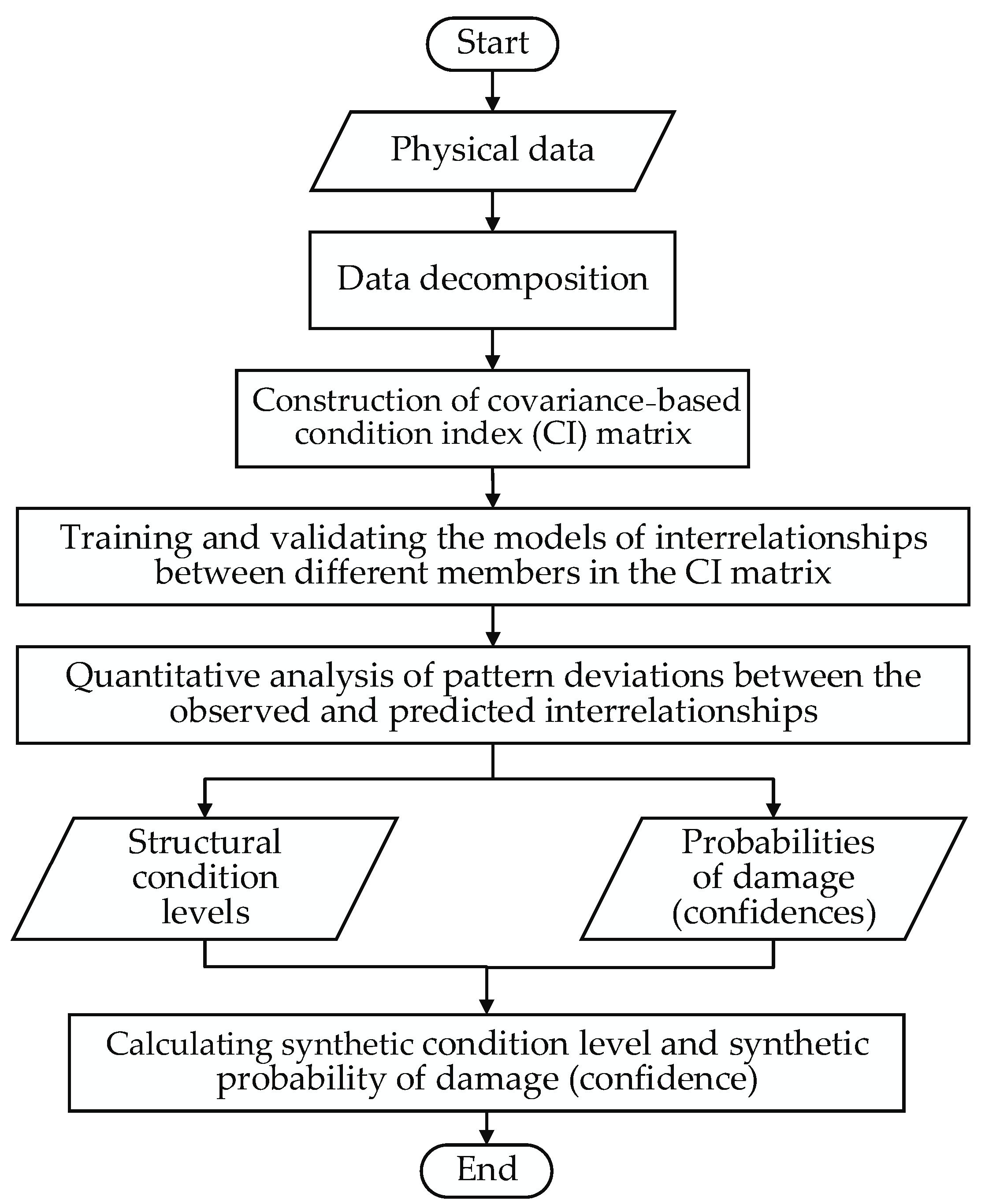
The proposed methodology includes three steps, namely the establishment of a covariance-based CI matrix after the time-frequency decomposition of responses, the training and validation of reference models of interrelationships between different members in the CI matrix, and quantitative assessment of the pattern differences between the observed and predicted interrelationships. The flowchart illustrating the proposed damage identification methodology is depicted in Figure 1. The CI matrix is formulated in Section 2.1, and the technique for reference model construction and quantitative assessment is described in Section 2.2.
2.1. Formulation of Condition Index
Considering the transient-release feature of acoustic-emission energy with crack progression, and inspired by the data fusion technique proposed by Wang et al. [49] for building a time-domain health condition index, a condition index based on time-frequency analysis and d matrix transformation is formulated herein. Specifically, the condition index is derived via the following process. The matrix for CI construction is obtained after performing time-frequency transformation on the signals collected by multiple sensors in the nth period. The response matrix containing covariance-based and amplitude-based segments can be expressed as:
where for the subscripts , , , , , and , is the total number of the time delay for computing covariances of multiple sensors, is also the total number of time slots for obtaining response segments of multiple sensors, and is the total number of frequency bands. To explore the latent relationships among the members, a Fourier transform is carried out on each column of , and the resultant matrix is denoted as .
A transformation matrix is designed for mapping the complex-valued matrix to a rail condition index. The condition index is denoted as , where , …, are column vectors associated with and , …, are column vectors associated with . The former are called covariance-based members and the latter are called amplitude-based members. The transformation matrix is a partitioned diagonal matrix transforming every part of as a column vector, and all column vectors are grouped as the index matrix . The current condition index and transformation matrix can be iteratively obtained by using Equations (2) and (3):
where is a small positive value for avoiding the ill-conditioned problem when solving the inverse of the matrix, is the initial value of and it uses a matrix in which all elements are one, and an adjustable weight is used to represent the initial health condition (i.e., intact condition). The transformation matrix is always computed by using healthy data. Therefore, if the condition index is found abnormal, the anomalous state of the condition index only comes from .
2.2. Construction of Reference Models for Damage Detection
To mine the underlying knowledge in healthy status, the relationships between different members in the CI matrix built by using healthy data are modeled. The CI matrix is composed of several covariance-based members as well as amplitude-based members, and the relationship between a member in one type and a member in the other type has not been exploited. This interrelationship between the two types of members in the CI can be described as:
where is additive random noise that is generally assumed as Gaussian in structural health monitoring, and the model output at an arbitrary point is intended to be predicted with pairs of training data . As each member of the CI is complex valued, the pairs of training data can be either the real or imaginary part of one column in the covariance-based members and that of another column in the amplitude-based members.
Various machine learning methods, such as neural network, support vector machine, and Bayesian regression, can be applied to build the models of anomaly-sensitive relationships between the two types of members in V. Sparse Bayesian regression is adopted for diminishing the overfitting problem, and is a combination of kernel functions, as shown in Equation (5).
where and denote the basis kernel function, and is the weight vector. The predicted output can be obtained as the product of kernel functions and the posterior estimation of the weight vector .
By using sensory data acquired when the structure is undamaged, the model governed by Equation (6) represents a normal interrelationship in healthy state. So, the model can be called a reference model and the prediction of a reference model can serve as a baseline. If the current pattern of the interrelationship built by using newly observed data deviates from the baseline pattern of the predicted interrelationship governed by Equation (6), an anomaly may be flagged.
The quantitative analysis relies on the philosophy that a relative change between the two types of members in the CI matrix can reflect damage existence, and the extent of the relative change or pattern deviation is associated with the severity level of damage. The quantification of the deviation between an observed interrelationship and a predicted interrelationship is made by Bayesian hypothesis testing of residuals via Bayes factor, due to its readily interpretable linkage with the severity of anomaly. For the rth set of damage-sensitive interrelationships (), the residual between the current observed interrelationship and the predicted inter-relationship is formulated as Equation (7).
where the subscripts obs and prd denote the observations and model predictions.
The Bayesian hypothesis testing is carried out on the mean of the residuals. If the mean value is approximately zero, the deviation of the observations from the model predictions is tolerable, representing a healthy state; otherwise, it indicates a damaged state. The ratio of the likelihoods between one hypothesis and the opposite hypothesis is defined as the Bayes factor [45,46,47]. The Bayes factor can be formulated as:
where stands for the damaged hypothesis, is the healthy hypothesis, and denotes the residual data. If the discrimination between the predicted baseline and the current observation is within a tolerable range, the Bayesian factor is smaller than 1, implying a health state. Otherwise, the damaged hypothesis is supported by the currently collected data ( > 1). The range of reflects the severity of discrimination. There are several intervals for the Bayes factor to assess the significance of discrimination or anomaly severity: for “barely worth mentioning’’ damage, for “substantial” damage, for “strong” damage, and for a “very strong” damage. The probability or confidence for the hypothesis testing of Gaussian residuals [48] is given as:
where stands for the probability or confidence, and and are the previous and the current Bayes factors obtained by Equation (8).
For the covariance-based and the amplitude-based damage-sensitive members in the CI matrix , there are interrelationships between the two types of members. Either the real part or the imaginary part of a member in the former type can be set as the input of a reference model, and either of them of a member in the latter type can be set as its output. Regarding the models and the related assessment results, a dilemma in decision-making may happen. To solve this problem, a synthetic Bayes factor is developed as:
where the subscript represents the synthetic result, the subscripts and stand for the covariance-based and the amplitude-based members respectively, and is the probability divided by the 2-norm of model error of the reference model. The synthetic probability of damage (confidence) can be formulated as Equation (11) by using the same weights as those in Equation (10).
3. Case Study
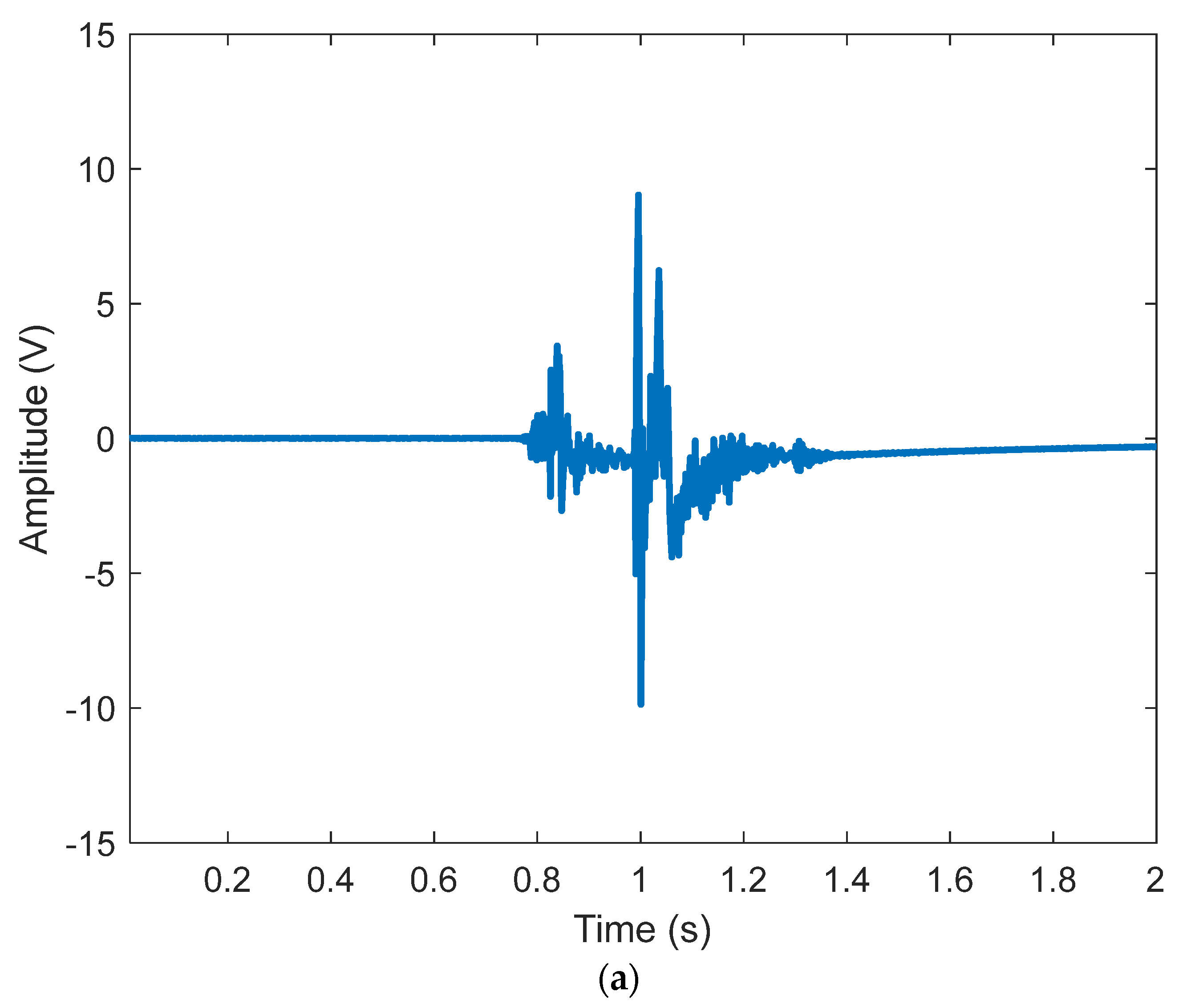
To validate the proposed method, a case study with three testing scenarios is performed using the monitoring data of an in-service railway turnout (Figure 2). A pair of PZT (Lead Zirconate Titanate) sensor arrays are installed symmetrically on the feet of two rails near the turnout ends. Monitoring data are collected from the turnout when it is healthy and becomes damaged, upon the passage of trains with different types, axle loadings, and speeds. For diminishing the influence of interference factors, the relative change between two members of the CI matrix is exploited for damage detection, rather than using the traditional approaches that compare a historical index (an index built with data acquired in a historically healthy state) with a current index (the same index built with new data acquired in an unknown state). The method formulated in Section 2 is conducted in this section. Wavelet packet analysis is carried out to obtain time-frequency components and construct the CI matrix. A typical response segment and four components after wavelet packet analysis are illustrated in Figure 3. The four components corresponding to 37.5–75.5, 75.5–112.5, 112.5–150, and 150–187.5 kHz are extracted for exploring the interrelationships between the covariance-based members and amplitude-based members of the CI matrix. They are called covariance-based member 1–member 4 and amplitude-based member 1–member 4 in accordance with the four frequency bands. As the members are complex-valued, the real parts are used to establish reference models of the interrelationships. As the procedure for anomaly identification using the proposed method is the same for the modeling and anomaly quantification of all interrelationships, detailed discussions are provided regarding some typical interrelationships.
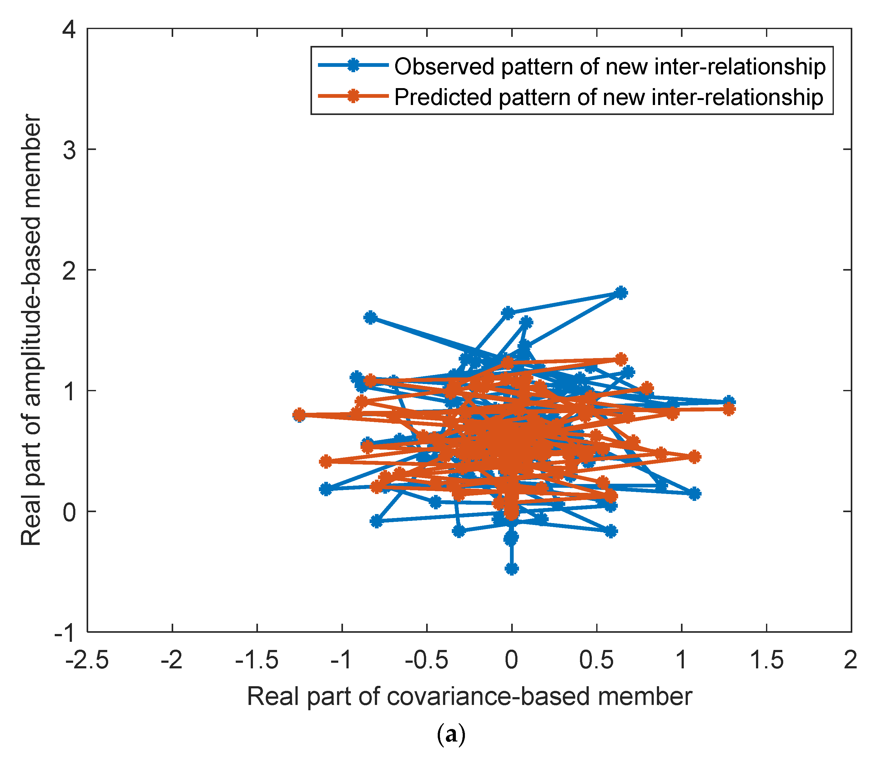
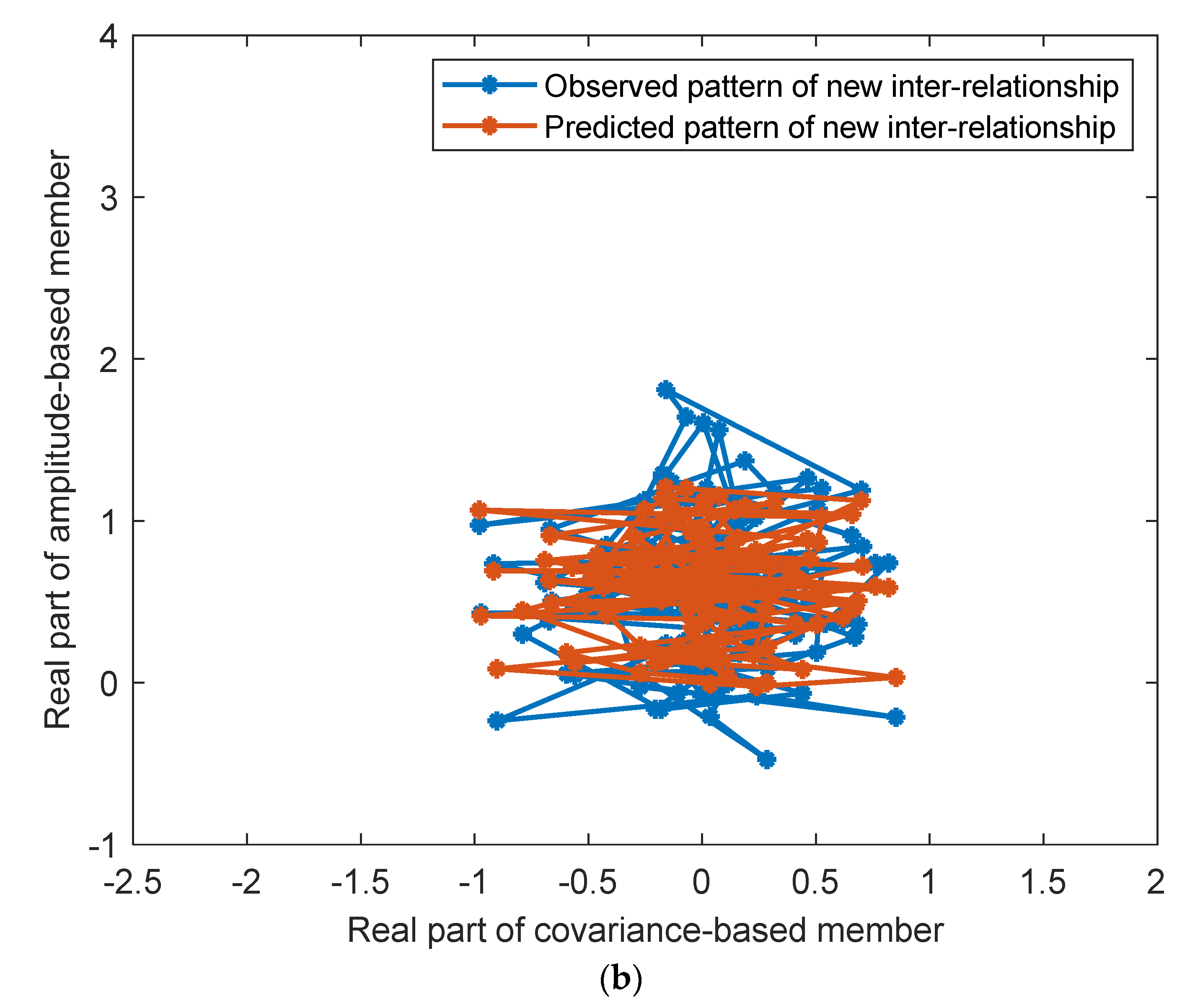
In the first scenario, model training is carried out and a large group of monitoring data acquired from a healthy turnout are employed to build the historical CI matrix. To explore the interrelationships latent in the CI matrix, two reference models of the interrelationships are constructed, including the model with the real part of covariance-based member 1 and that of amplitude-based member 2 as its input and output, and the model with the real part of covariance-based member 4 and that of amplitude-based member 2 as its input and output. The observed and predicted patterns of the interrelationships from the real part of covariance-based member 1 to that of amplitude-based member 2 are depicted in Figure 4a. The observed and predicted patterns of the interrelationships from the real part of covariance-based member 4 to that of amplitude-based member 2 are illustrated in Figure 4b. In Figure 4a,b, historical patterns (blue lines) are highly accordant with the predicted patterns (orange lines), verifying the reference models. It is also found that the two interrelationships possess reticular patterns largely located in the upper-half plane.
In the second scenario, a small group of monitoring data are imported for building a new CI matrix, and the real parts of covariance-based member 1 and member 4 are respectively fed into the two reference models, yielding new predictions for the real part of amplitude-based member 2. The observed and the predicted patterns are shown in Figure 5 for comparison. Figure 5a displays the pattern comparison for the interrelationship from covariance-based member 1 to the amplitude-based member 2. Figure 5b exhibits the comparison between the observed and predicted patterns for the interrelationship from covariance-based member 4 to the amplitude-based member 2. It can be seen that the observed and the predicted patterns are still reticular in the upper-half plane. In addition, the observed and predicted patterns in Figure 5a,b are almost entirely located inside the historical patterns in Figure 4a,b. Slight deviations between the observed and the predicted patterns are quantitatively assessed by the Bayes factor. The values of Bayes factor for the differences between the blue and orange reticular patterns are respectively 0.1 and 0.6, with the probabilities of damage (confidences) being 1.1% and 5.3%. According to Equations (10) and (11), the synthetic Bayes factor is computed as 0.3, with the synthetic probability (confidence) being 2.9%. The pair of synthetic results, namely the synthetic Bayes factor and synthetic probability, favor the hypothesis of “healthy state”. This situation is accordant with the actual rail condition of the turnout. This new dataset is incorporated into the database for updating the historical CI matrix.
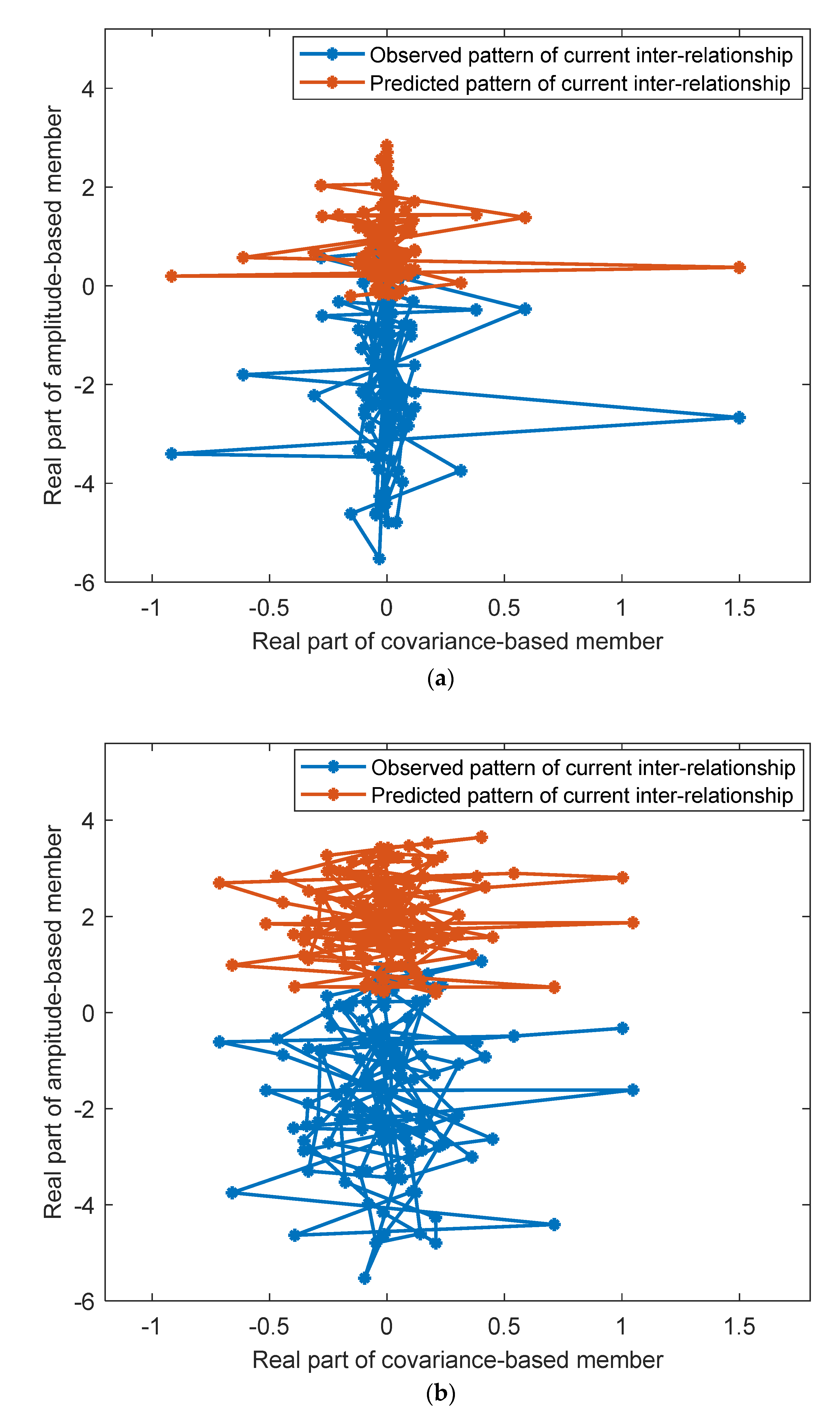
In the third scenario, another group of new data is imported to build the current CI matrix and predict the current health condition by using the two updated models. Based on the same procedure as that in the second scenario, the real parts of covariance-based member 1 and member 4 in the current CI matrix are fed into the two models, generating current predictions for real part of amplitude-based member 2. The observed and the predicted patterns are shown in Figure 6 for comparison. As illustrated in Figure 6a,b, significant deviations between the currently observed and predicted patterns are witnessed; the two observed patterns (blue lines) hold reticular patterns, but these patterns are located mainly in the lower half-plane. The values of the Bayes factor for the deviations in the two patterns are respectively 10.5 and 40.4, with the probabilities of damage (confidences) being 50.9% and 78.6%. According to Equations (10) and (11), the synthetic Bayes factor is computed as 26.2, with the synthetic probability of damage (confidence) being 65.4%. The synthetic factor and probability advocate the hypothesis of “damaged state” and the condition is identified as strongly damaged. Meanwhile, it is found that a deep crack occurs in the rail head of the turnout tip. The identified condition agrees very well with the real condition of the turnout rail.
4. Discussions
After model training and validation conducted in the first scenario, the quantitative assessment results in the second and third scenarios with different conditions of the turnout rail are summarized in Table 1. These results correspond to Figure 5 and Figure 6 respectively, in the second and third scenarios and they are consistent with the real conditions of the railway turnout, verifying the effectiveness of the proposed method. Compared with other machining learning methods, the Bayesian method combining sparse Bayesian regression and Bayes factor evaluates the turnout structural condition in a probabilistic manner, rather than providing a deterministic result. In addition, different from traditional approaches that compare a historical index with a current index, this study exploits the concealed interrelationships between different types of members in the current CI matrix. This helps to avoid the false positives in the traditional approaches which are induced by the normal change in an index accompanied with the structural evolution and the variation in the influential factors.
However, the probability of damage is not high because the number of monitoring datasets in the damaged scenario is not enough for updating and enhancing the probabilistic results. In addition, it is generally not allowed to deploy plenty of electric sensors in railway engineering despite the high sensitivity of the installed sensors to acoustic emission waves. Fiber optic sensors together with a high-speed interrogator are more suitable when more sensors are desired for acquiring the waves.
5. Conclusions
A quantitative condition evaluation method for the crack-alike damage identification of in-service turnout rails has been developed and validated in this study. It is composed of three elements, including a covariance-based structural condition index that is built with time-frequency components of responses for taking advantage of acoustic emission waves induced by crack initiation and progression, a series of baseline patterns described by Bayesian models and reflecting the interrelationships between two types of members in the CI matrix, and an assessment technique synthetically quantifying the deviations between the baseline patterns and the observed patterns by using designed weights. A case study with different testing scenarios was conducted with the use of monitoring data acquired from an in-service turnout, for examining the performance of the proposed method. It was found that the interrelationships between the two types of index members exhibit reticular patterns, the predicted and observed patterns of the inter-relationships are consistent with each other very well when the inputted new data are collected from the turnout in healthy state, and great deviations occur in the predicted and observed patterns when the inputted new data are acquired from the turnout in strongly damaged state. The synthetic assessment results in the different testing scenarios are in accordance with the real conditions of the turnout. These findings demonstrate the effectiveness of the proposed method in identifying damage existence and severity. Both the severity levels and probabilistic confidences are provided, yielding a more objective assessment for the in-service structure under uncertain influential factors. As the proposed method is formulated without the use of a physical model and the measurement of loadings, it is potentially expandable to wider applications of various engineering structures for crack-alike damage identification.
Author Contributions
Methodology and writing—original draft preparation, J.-F.W.; investigation and writing—review and editing, J.-F.L.; validation and writing—review and editing, Y.-L.X. All authors have read and agreed to the published version of the manuscript.
Funding
The authors wish to acknowledge the support from the National Natural Science Foundation of China (Grant No. 52008258), Guangdong Major Talent Program (Grant No. 2021QN02Z709), Shenzhen Science and Technology Program (Grant No. KQTD20180412181337494), the Shenzhen Sustainable Development Science and Technology Project (Grant No. KCXFZ20201221173608023), China Earthquake Administration’s Science for Earthquake Resilience Project (Grant No. XH204702), Shenzhen Science and Technology Program (Grant No. JSGG20210802093207022) and Shenzhen Key Laboratory of Structure Safety and Health Monitoring of Marine Infrastructures (Grant No. ZDSYS20201020162400001).
Data Availability Statement
The data are not publicly available due to privacy restrictions.
Conflicts of Interest
The authors declare no conflict of interest.
References
- Ishak, M.F.; Dindar, S.; Kaewunruen, S. Safety–based maintenance for geometry restoration of railway turnout systems in various operational environments. In Proceedings of the 21st National Convention on Civil Engineering, Songkhla, Thailand, 28–30 June 2016. [Google Scholar]
- Dindar, S.; Kaewunruen, S.; An, M. Identification of appropriate risk analysis techniques for railway turnout systems. J. Risk Res. 2016, 21, 974–995. [Google Scholar] [CrossRef]
- Dindar, S.; Kaewunruen, S. Assessment of turnout–related derailments by various causes. In GeoMEast 2017: Recent Developments in Railway Track and Transportation Engineering, Proceedings of the International Congress and Exhibition “Sustainable Civil Infrastructures: Innovative Infrastructure Geotechnology”, Sharm El–Sheikh, Egypt, 11–15 November 2017; Pombo, J., Jing, G., Eds.; Springer: Cham, Switzerland, 2018. [Google Scholar]
- Liu, X.; Saat, R.; Barkan, C.P. Analysis of causes of major train derailment and their effect on accident rates. Transp. Res. Rec. 2012, 2289, 154–163. [Google Scholar] [CrossRef]
- 49 CFR Part 213; Track Safety Standards. U.S. Department of Transportation, Federal Railroad Administration: Washington, DC, USA, 2009.
- Chen, X. Research on the Rail Damage of Railway Turnout. Master’s Thesis, China Academy of Railway Sciences, Beijing, China, 2019. [Google Scholar]
- Wang, P.; Chen, R.; Xu, J.M.; Ma, X.C.; Wang, J. Theories and engineering practices of high–speed railway turnout system: Survey and review. J. Southwest Jiaotong Univ. 2016, 51, 357–372. [Google Scholar]
- Su, Z.; Ye, L. Identification of Damage Using Lamb Waves: From Fundamentals to Applications; Springer: London, UK, 2009. [Google Scholar]
- Sysyn, M.; Gerber, U.; Nabochenko, O.; Kovalchuk, V. Common crossing fault prediction with track based inertial measurements: Statistical vs. mechanical approach. Pollack Period. 2019, 14, 15–26. [Google Scholar] [CrossRef]
- Sysyn, M.P.; Kovalchuk, V.V.; Jiang, D. Performance study of the inertial monitoring method for railway turnouts. Int. J. Rail Transp. 2019, 7, 103–116. [Google Scholar] [CrossRef]
- Sysyn, M.; Gruen, D.; Gerber, U.; Nabochenko, O.; Kovalchuk, V. Turnout monitoring with vehicle based inertial measurements of operational trains: A machine learning approach. Komun. Ved. Listy Žilinskej Univ. Žiline 2019, 1, 42–48. [Google Scholar] [CrossRef]
- Kovalchuk, V.; Sysyn, M.; Gerber, U.; Nabochenko, O.; Zarour, J.; Dehne, S. Experimental investigation of the influence of train velocity and travel direction on the dynamic behavior of stiff common crossings. Facta Univ. Ser. Mech. Eng. 2019, 17, 345–356. [Google Scholar] [CrossRef]
- Sysyn, M.P.; Nabochenko, O.S.; Kluge, F.; Kovalchuk, V.V.; Pentsak, A. Common crossing structural health analysis with track–side monitoring. Commun. Sci. Lett. Univ. Zilina 2019, 21, 77–84. [Google Scholar] [CrossRef]
- Sysyn, M.; Gerber, U.; Nabochenko, O.; Li, Y.; Kovalchuk, V. Indicators for common crossing structural health monitoring with track–side inertial measurements. Acta Polytech. 2019, 59, 170–181. [Google Scholar] [CrossRef]
- Sysyn, M.; Nabochenko, O.; Kovalchuk, V.; Gruen, D.; Pentsak, A. Improvement of inspection system for common crossings by track side monitoring and prognostics. Struct. Monit. Maint. 2019, 6, 219–235. [Google Scholar]
- Sysyn, M.; Gerber, U.; Kluge, F.; Nabochenko, O.; Kovalchuk, V. Turnout remaining useful life prognosis by means of on–board inertial measurements on operational trains. Int. J. Rail Transp. 2020, 8, 347–369. [Google Scholar] [CrossRef]
- Bassim, M.N.; Lawrence, S.S.; Liu, C.D. Detection of the onset of fatigue crack growth in rail steels using acoustic emission. Eng. Fract. Mech. 1994, 47, 207–214. [Google Scholar] [CrossRef]
- Kostryzhev, A.G.; Davis, C.L.; Roberts, C. Detection of crack growth in rail steel using acoustic emission. Ironmak. Steelmak. 2013, 40, 98–102. [Google Scholar] [CrossRef]
- Wang, J.H. Monitoring system for rail fracture and damage of heavy haul railway turnout based on bispectrum. Railw. Eng. 2017, 6, 130–134. [Google Scholar]
- Wang, J.F.; Liu, X.Z.; Ni, Y.Q. A Bayesian probabilistic approach for acoustic emission based rail condition assessment. Comput. Aided Civ. Infrastruct. Eng. 2018, 33, 21–34. [Google Scholar] [CrossRef]
- Zain, M.S.M.; Jamaludin, N.; Sajuri, Z.; Yusof, M.F.M.; Hanafi, Z.H. Acoustic emission study of fatigue crack growth in rail track material. In Proceedings of the National Conference in Mechanical Engineering Research and Postgraduate Studies (2nd NCMER 2010), Pahang, Malaysia, 3–4 December 2010. [Google Scholar]
- Zhang, J.; Ma, Y.L. Comparison of three fatigue crack growth rate models. Res. Explor. Lab. 2012, 31, 35–38. [Google Scholar]
- Shiotani, T.; Li, Z.; Yuyama, S.; Ohtsu, M. Application of the AE improved b–value to quantitative evaluation of fracture process in concrete materials. J. Acoust. Emiss. 2001, 19, 118–133. [Google Scholar]
- Shahidan, S.; Nor, N.M.; Bunnori, N.M. Analysis methods of Acoustic Emission signal for monitoring of reinforced concrete structure: A review. In Proceedings of the 2011 IEEE 7th International Colloquium on Signal Processing and its Applications, Penang, Malaysia, 4–6 March 2011. [Google Scholar]
- Chen, Z.G. Damage Identification and Deterioration Evaluation of RC Based on Acoustic Emission Technology. Ph.D. Thesis, Zhejiang University, Hangzhou, China, 2018. [Google Scholar]
- Gu, A.; Sun, L.; Liang, J.; Han, W. Acoustic emission characteristics based on energy mode of IMFs. In Advances in Acoustic Emission Technology, Proceedings of The World Conference on Acoustic Emission, Xi’an, China, 10–13 October 2017; Shen, G., Zhang, J., Wu, Z., Eds.; Springer: Berlin/Heidelberg, Germany, 2017. [Google Scholar]
- Shiotani, T. Recent advances of AE technology for damage assessment of infrastructures. J. Acoust. Emiss. 2012, 30, 76–99. [Google Scholar]
- Sun, H. Damage Characteristics Analysis of T700 Carbon Fiber Composite Based on Modal Acoustic Emission. Master’s Thesis, Northeast Petroleum University, Daqing, China, 2019. [Google Scholar]
- Zhang, W.; Geng, J.; Xu, Y. Application of modal acoustic emission technique for recognition of corrosion severity on a thin plate. In Advances in Acoustic Emission Technology, Proceedings of The World Conference on Acoustic Emission, Xi’an, China, 10–13 October 2017; Shen, G., Zhang, J., Wu, Z., Eds.; Springer: Berlin/Heidelberg, Germany, 2017. [Google Scholar]
- Zárate, B.A.; Caicedo, J.M.; Yu, J.; Ziehl, P. Model updating and prognosis of acoustic emission data in compact test specimens under cyclic loading. In Proceedings of the Nondestructive Characterization for Composite Materials, Aerospace Engineering, Civil Infrastructure, and Homeland Security, San Diego, CA, USA, 6–10 March 2011; SPIE: Bellingham, WA, USA, 2011; Volume 7983. [Google Scholar]
- Masoud, R.; Mohammad, M. Quantitative methods for structural health management using in situ acoustic emission monitoring. Int. J. Fatigue 2013, 49, 81–89. [Google Scholar]
- Masoud, R.; Mohammad, M. A recursive Bayesian framework for structural health management using online monitoring and periodic inspections. Reliab. Eng. Syst. Saf. 2013, 112, 154–164. [Google Scholar]
- Chai, M.; Zhang, Z.; Duan, Q.; Song, Y. Assessment of fatigue crack growth in 316ln stainless steel based on acoustic emission entropy. Int. J. Fatigue 2018, 109, 145–156. [Google Scholar] [CrossRef]
- Zachary, K.; Walter, H.; James, S. Crack propagation analysis using acoustic emission sensors for structural health monitoring systems. Sci. World J. 2013, 2013, 823603. [Google Scholar]
- Niu, Y.Y.M.; Wong, Y.S.; Hong, G.S. An intelligent sensor system approach for reliable tool flank wear recognition. Int. J. Adv. Manuf. Technol. 1998, 14, 77–84. [Google Scholar] [CrossRef]
- Yao, Y.X.; Li, X.; Yuan, Z.J. Tool wear detection with fuzzy classification and wavelet fuzzy neural network. Int. J. Mach. Tools Manuf. 1999, 39, 1525–1538. [Google Scholar] [CrossRef]
- Luo, Z.C.; Bi, A.R.; Wang, X.W. Corrosion prediction of high sulfur gas–oil mixed transmission pipelines based on PCA–SVM. China Saf. Sci. J. 2016, 26, 85–90. [Google Scholar]
- Lin, L.; Wang, H.; Zhou, Y. Research on the Identification of Crack Status Through the Axle Acoustic Emission Signal Based on Local Mean Decomposition and Grey Correlation Analysis. In Advances in Acoustic Emission Technology, Proceedings of The World Conference on Acoustic Emission, Xi’an, China, 10–13 October 2017; Shen, G., Zhang, J., Wu, Z., Eds.; Springer: Berlin/Heidelberg, Germany, 2017. [Google Scholar]
- Zhang, F.L.; Gu, D.K.; Li, X.; Ye, X.W.; Peng, H. Structural damage detection based on fundamental Bayesian two–stage model considering the modal parameters uncertainty. Struct. Health Monit. 2023, 22, 2305–2324. [Google Scholar] [CrossRef]
- Qiu, S.; Wu, Z.; Li, M.; Yang, H.; Yue, F. Shape monitoring and damage identification in stiffened plates using inverse finite element method and Bayesian learning. J. Vib. Control 2023, 29, 2489–2500. [Google Scholar] [CrossRef]
- Huang, K.; Yuen, K.V. Hierarchical outlier detection approach for online distributed structural identification. Struct. Control Health Monit. 2020, 27, e2623. [Google Scholar] [CrossRef]
- Wan, H.P.; Ren, W.X. Stochastic model updating utilizing Bayesian approach and Gaussian process model. Mech. Syst. Signal Process. 2016, 70–71, 245–268. [Google Scholar] [CrossRef]
- Wang, Q.A.; Dai, Y.; Ma, Z.G.; Wang, J.F.; Lin, J.F.; Ni, Y.Q.; Ren, W.X.; Jiang, J.; Yang, X.; Yan, J.R. Towards high–precision data modelling of SHM measurements using an improved sparse Bayesian learning scheme with strong generalization ability. Struct. Health Monit. 2023, 23, 588–604. [Google Scholar] [CrossRef]
- Lindely, D.V.; Smith, A.F. Bayes estimates for linear models. J. R. Stat. Soc. Ser. B 1972, 34, 1–41. [Google Scholar] [CrossRef]
- Aitkin, M. Posterior Bayes factors. J. R. Stat. Soc. Ser. B 1991, 53, 111–142. [Google Scholar] [CrossRef]
- Kass, R.; Raftery, A. Bayes factors. J. Am. Stat. Assoc. 1995, 90, 773–795. [Google Scholar] [CrossRef]
- Jiang, X.; Mahadevan, S. Bayesian wavelet methodology for structural damage detection. Struct. Control Health Monit. 2008, 15, 974–991. [Google Scholar] [CrossRef]
- Sankararaman, S.; Mahadevan, S. Bayesian methodology for diagnosis uncertainty quantification and health monitoring. Struct. Control Health Monit. 2013, 20, 88–106. [Google Scholar] [CrossRef]
- Wang, P.; Youn, B.D.; Hu, C. A generic probabilistic framework for structural health prognostics and uncertainty management. Mech. Syst. Signal Process. 2012, 28, 622–637. [Google Scholar] [CrossRef]
Figure 1.
A flowchart of the proposed methodology.

Figure 2.
The railway turnout with symmetrical areas for installing sensors.
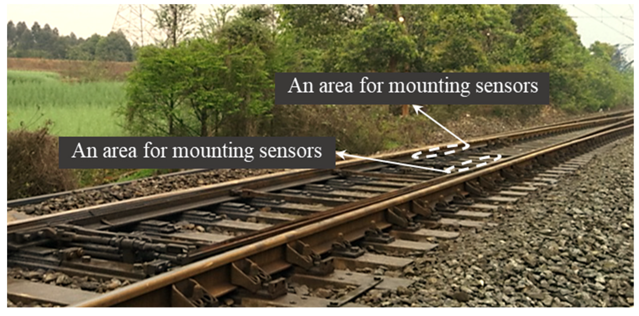
Figure 3.
A typical response segment and its components after wavelet packet analysis. (a) A segment of a typical response. (b) The four components of a typical response.
Figure 3.
A typical response segment and its components after wavelet packet analysis. (a) A segment of a typical response. (b) The four components of a typical response.

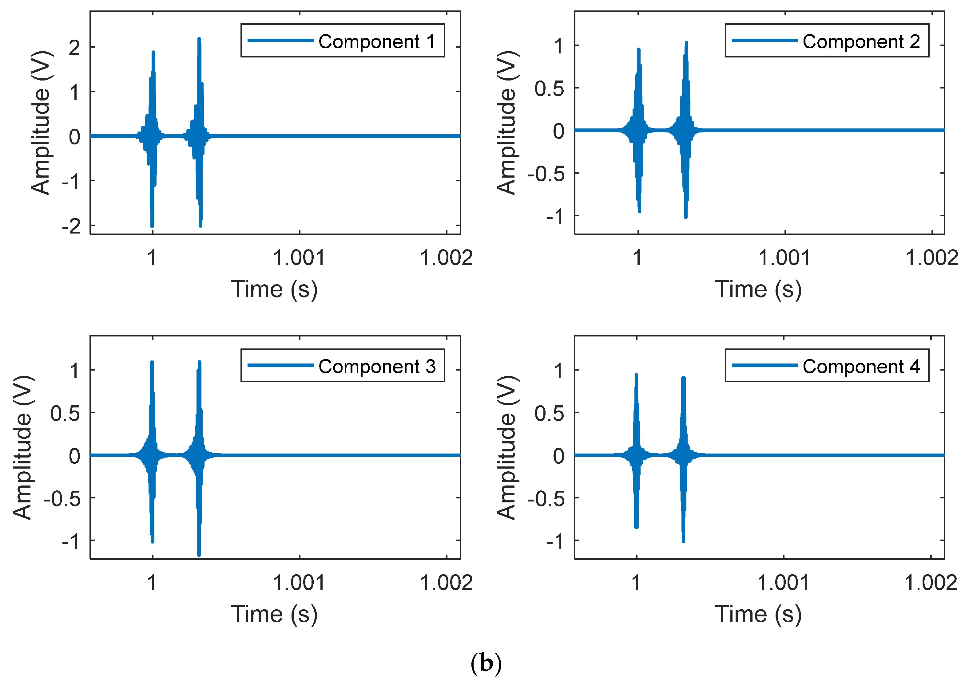
Figure 4.
The comparison between observed and predicted historical patterns for model validation (the first scenario). (a) The relationship between covariance-based member 1 and amplitude-based member 2 in the historical CI matrix. (b) The relationship between covariance-based member 4 and amplitude-based member 2 in the historical CI matrix.
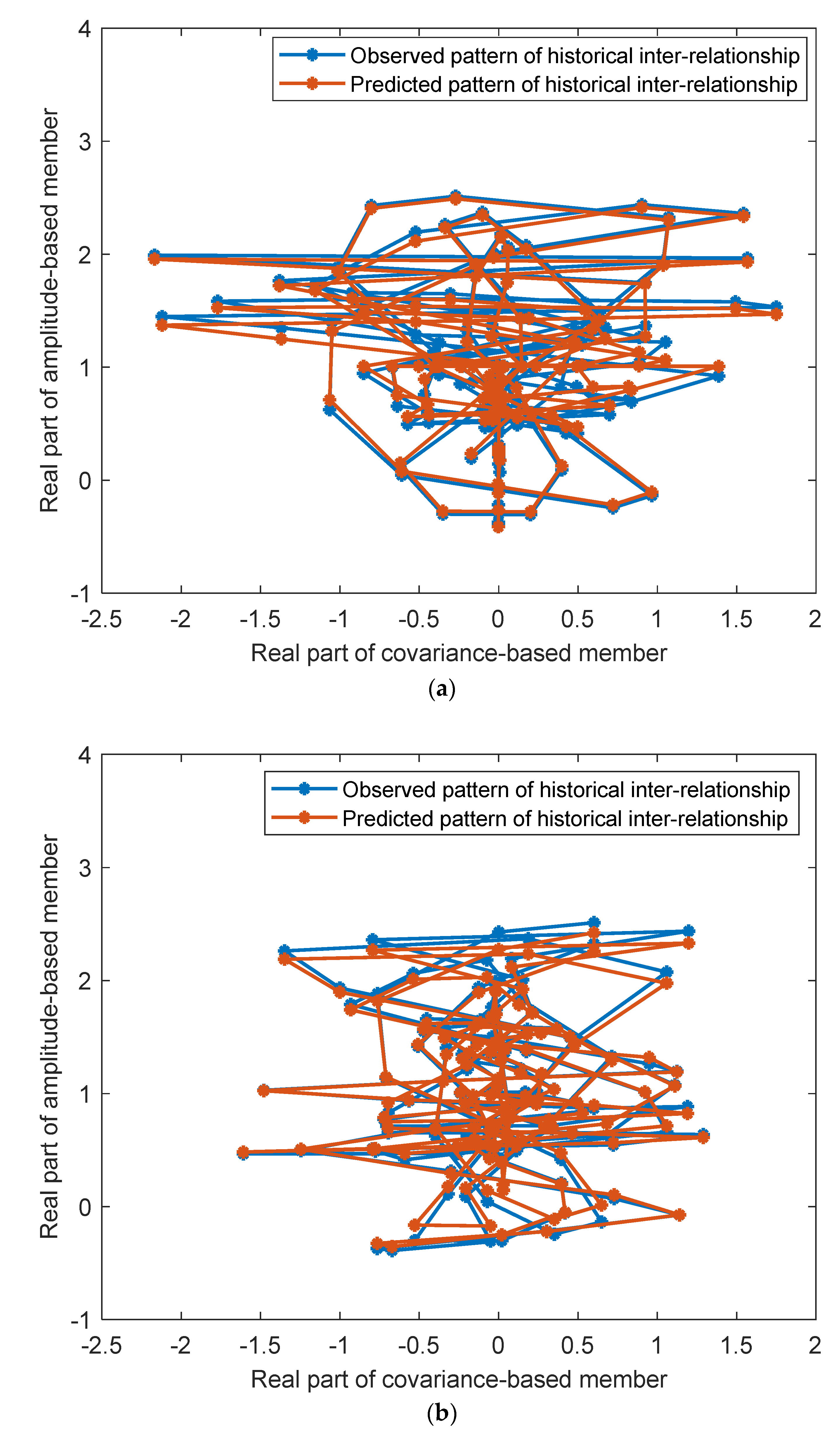
Figure 5.
The comparison between observed and predicted new patterns for anomaly detection (the second scenario). (a) The relationship between covariance-based member 1 and amplitude-based member 2 in the new CI matrix. (b) The relationship between covariance-based member 4 and amplitude-based member 2 in the new CI matrix.


Figure 6.
The comparison between observed and predicted current patterns for anomaly detection (the third scenario). (a) The relationship between covariance-based member 1 and amplitude-based member 2 in the current CI matrix. (b) The relationship between covariance-based member 4 and amplitude-based member 2 in the current CI matrix.

Table 1.
Bayes factors and probabilities of damage (confidences).
| Bayes Factor (Probability of Damage) for the Interrelationship 1 | Bayes Factor (Probability of Damage) for the Interrelationship 2 | Synthetic Bayes Factor (Synthetic Probability) | |
|---|---|---|---|
| Scenario 2 | 0.1 (1.1%) | 0.6 (5.3%) | 0.3 (2.9%) |
| Scenario 3 | 10.5 (50.9%) | 40.4 (78.6%) | 26.2 (65.4%) |
Disclaimer/Publisher’s Note: The statements, opinions and data contained in all publications are solely those of the individual author(s) and contributor(s) and not of MDPI and/or the editor(s). MDPI and/or the editor(s) disclaim responsibility for any injury to people or property resulting from any ideas, methods, instructions or products referred to in the content. |
© 2023 by the authors. Licensee MDPI, Basel, Switzerland. This article is an open access article distributed under the terms and conditions of the Creative Commons Attribution (CC BY) license (https://creativecommons.org/licenses/by/4.0/).
Share and Cite
MDPI and ACS Style
Wang, J.-F.; Lin, J.-F.; Xie, Y.-L. Damage Identification of Turnout Rail through a Covariance-Based Condition Index and Quantitative Pattern Analysis. Infrastructures 2023, 8, 176. https://doi.org/10.3390/infrastructures8120176
AMA Style
Wang J-F, Lin J-F, Xie Y-L. Damage Identification of Turnout Rail through a Covariance-Based Condition Index and Quantitative Pattern Analysis. Infrastructures. 2023; 8(12):176. https://doi.org/10.3390/infrastructures8120176
Chicago/Turabian StyleWang, Jun-Fang, Jian-Fu Lin, and Yan-Long Xie. 2023. "Damage Identification of Turnout Rail through a Covariance-Based Condition Index and Quantitative Pattern Analysis" Infrastructures 8, no. 12: 176. https://doi.org/10.3390/infrastructures8120176