
Deep Learning-Based Steel Bridge Corrosion Segmentation and Condition Rating Using Mask RCNN and YOLOv8

1
Department of Civil and Environmental Engineering, University of Maine, Orono, ME 04469, USA
2
Department of Engineering, University of Science and Culture, Tehran 1461968151, Iran
*
Author to whom correspondence should be addressed.
Infrastructures 2024, 9(1), 3; https://doi.org/10.3390/infrastructures9010003
Submission received: 13 October 2023
/
Revised: 5 December 2023
/
Accepted: 7 December 2023
/
Published: 20 December 2023
(This article belongs to the Special Issue Structural Health Monitoring and Performance Evaluation of Bridges and Structural Elements)
Abstract
:The application of deep learning (DL) algorithms has become of great interest in recent years due to their superior performance in structural damage identification, including the detection of corrosion. There has been growing interest in the application of convolutional neural networks (CNNs) for corrosion detection and classification. However, current approaches primarily involve detecting corrosion within bounding boxes, lacking the segmentation of corrosion with irregular boundary shapes. As a result, it becomes challenging to quantify corrosion areas and severity, which is crucial for engineers to rate the condition of structural elements and assess the performance of infrastructures. Furthermore, training an efficient deep learning model requires a large number of corrosion images and the manual labeling of every single image. This process can be tedious and labor-intensive. In this project, an open-source steel bridge corrosion dataset along with corresponding annotations was generated. This database contains 514 images with various corrosion severity levels, gathered from a variety of steel bridges. A pixel-level annotation was performed according to the Bridge Inspectors Reference Manual (BIRM) and the American Association of State Highway and Transportation Officials (AASHTO) regulations for corrosion condition rating (defect #1000). Two state-of-the-art semantic segmentation algorithms, Mask RCNN and YOLOv8, were trained and validated on the dataset. These trained models were then tested on a set of test images and the results were compared. The trained Mask RCNN and YOLOv8 models demonstrated satisfactory performance in segmenting and rating corrosion, making them suitable for practical applications.
1. Introduction
In the United States, more than 40 percent of all bridges are built of steel (U.S. National Bridge Inventory (NBI)), and corrosion is a major factor in the deterioration of these structures. Each year, the federal government and state Departments of Transportation (DOTs) spend billions of dollars on bridge rehabilitation and maintenance due to corrosion [1]. Corrosion reduces the effective cross-sections of critical structural components and subsequently decreases the axial, bending, and fatigue strength, which can lead to the failure of individual elements and entire structures. In order to detect and mitigate corrosion damage, regular inspection is essential. Steel structural elements must be evaluated in terms of the initiation of corrosion, section loss, or any other possible adverse effect on the strength or serviceability of structural elements. Since maintenance decisions mainly depend on the information collected during inspection, accurate bridge inspection and data analysis is important in optimizing bridge maintenance strategies and avoiding unnecessary repair costs.
The manual inspection of the bridge is always time-consuming and the result is inconsistent, subjective, and largely dependent on the experience and judgment of the inspector [2,3]. In addition, traditional bridge inspection is costly and associated with safety risks for the inspection crew and public. Unmanned aerial vehicles (UAVs) have proven to be a viable and safer solution to perform such inspections in many adverse conditions by flying up close to the structures and taking large numbers of high-resolution images from multiple angles [4,5]. Integrating UAVs with artificial intelligence (AI) in infrastructure inspections, particularly in tasks like defect detection, classification, and segmentation, offers significant benefits in terms of reduced time and costs and the enhanced accuracy of the results [6,7]. This study has focused on automated corrosion classification and condition rating to address the inefficiencies of traditional inspection.
Corrosion exhibits two main visual characteristics: a rough surface texture and a red color spectrum. These properties have been used for corrosion detection by applying feature-based classification techniques [8]. Machine learning-based corrosion detection, such as support vector machines (SVM) and random forest, requires experts to manually define relevant features. The algorithm then learns to detect corrosion based on these features. For instance, in a study by Khayatazad et al. (2020), the authors quantified and combined roughness and color for corrosion detection. The uniformity metric calculated from the gray-level co-occurrence matrix and the histogram of corrosion-representative colors were used to analyze roughness and color, respectively [9]. These techniques require manual feature engineering, which may not capture all variations in the data, and the quality of the manually selected features might affect performance of the algorithm. Image processing techniques such as histogram equalization and edge detection mitigate the need for the manual adjustment of threshold parameters, but they still require predefined rules to extract features directly from the images. The designed features may lack robustness when faced with diverse variations, leading to a significant decrease in recognition accuracy if the algorithm fails to effectively capture the advanced features present in the images [10]. Deep learning-based (DL) approaches automatically learn hierarchical features from raw data and adapt the learned features, effectively reducing the need for human intervention. DL-based techniques can handle complex, unstructured data and often achieve state-of-the-art performance. Convolutional neural networks (CNNs) are a class of deep neural networks, most commonly applied to analyze images [11]. CNNs have been used for object detection, classification, and segmentation and consistently exhibit remarkable performance compared to traditional classification algorithms. Petricca et al. (2016) presented a comparison between computer vision techniques and CNNs for automatic metal corrosion detection. The authors classified the image pixels based on the specific color components. The findings indicated that the deep learning approach achieved more uniform results and significantly higher accuracy compared to computer vision techniques [12]. Some studies have evaluated the performance of CNNs with different architectures in corrosion detection. Atha and Jahanshahi (2018) evaluated VGG and ZF Net, two different architectures of CNN, for corrosion detection. The authors also proposed two CNN architectures specifically designed for corrosion detection, namely Corrosion7 and Corrosion5. It was shown that the deeper architecture, VGG16, performed better in terms of accuracy than a smaller network such as ZF Net. The authors achieved 96.68% mean precision using 926 images. However, only clearly visible surface images were considered in this study [13]. Jin Lim et al. (2021) applied Faster RCNN with RGB and thermographic images for steel bridge corrosion inspection. They achieved an average precision (AP) value of 88% for surface and subsurface corrosion detection [14].
While corrosion detection is concerned with identifying the presence and location of corrosion in an image using bounding boxes, segmentation is focused on the pixel-level classification and delineation of object boundaries. Long et al. (2015) introduced fully convolutional networks (FCNs) as the first deep learning-based technique to perform the segmentation task, and since then, many image segmentation techniques, such as U-Net [15], DeepLab [16], PSPNet [17], SegNet [18], and Mask RCNN [19], have been developed. Each of these techniques has unique architectural features, which make them suitable for different image segmentation tasks. Recently, Ta et al. (2022) utilized the Mask RCNN algorithm, an instance segmentation approach, for the detection of corroded bolts. The model was able to accurately detect corrosion in the tested structure. The accuracy of the model declined along with the image capturing distance [20]. Nash et al. (2018) proposed a modified VGG-16 architecture to perform the pixel-level segmentation of corrosion. Neither of the models trained on small and large datasets achieved human-level accuracy for corrosion detection [21]. In their study, Rahman et al. (2021) proposed a semantic CNN model for corrosion detection and segmentation. The authors proposed a corrosion evaluation method based on the grayscale value for the classification of each pixel of a corrosion segment into heavy, medium, and light corrosion categories [8].
For the problem of bridge inspection, inspectors are responsible for assigning corrosion condition states to the corroded structural elements according to the BIRM [22] and American Association of State Highway and Transportation Officials (AASHTO) regulations [23]. Table 1 demonstrates these condition states. The number of studies that use DL-based methods to evaluate and assign standardized condition states to the corroded areas in the image is very limited. In a recent study, Munawar et al. (2022) divided the images into four corrosion levels, no corrosion (negative class), low-level corrosion (images having less than 5% of corroded pixels), medium-level corrosion (images having less than 15% of corroded pixels), and high-level corrosion (images having more than 15% of corroded pixels) [24], based on the number of corroded pixels. Notably, this classification method differs from the approach suggested by the Bridge Inspection Reference Manual (1), which recommends assessing the corrosion condition based on the severity of the corrosion.
To address the need for a practical corrosion condition rating approach, in the current study, we trained two DL-based corrosion segmentation algorithms to automatically rate the corroded areas and assign corrosion severity levels to them. The required corrosion images for the training of the algorithms were collected and annotated according to the AASHTO and BIRM regulations. The acquired corrosion images and corresponding annotations have been made openly accessible online and provide a resource for the training of future corrosion and condition rating models [25].
2. Materials and Methods
2.1. Image Acquisition and Annotation
A Nikon D750 camera and a DJI Mini drone were used to gather 514 high-quality corrosion images. These images were taken from steel bridge components such as girders and supports. To mitigate the risk of collision and ensure the safety of both the drone and the structure being inspected, the drone maintained a distance of more than one meter from the structure. Images were captured from multiple angles to provide a comprehensive view of the corroded areas. The blurry and dark images were removed from the dataset to maintain the overall quality of the input training data. Supervised learning algorithms such as Mask RCNN and YOLOv8 rely on labeled data for effective training; therefore, the collected images needed to be annotated. Annotation involves assigning each image with detailed labels specifying the boundaries or areas of interest. Pixel-wise annotation is time-consuming and challenging due to several factors. The smooth boundaries of corrosion make it difficult to accurately outline the damage, leading to potential inconsistencies. Additionally, the lack of distinct characteristics in corrosion severity makes it challenging to classify and annotate them correctly. Moreover, distinguishing actual corrosion from other visual artifacts, like dark backgrounds, dirt, or smudges, adds another layer of complexity to the annotation task. To address these challenges, the annotations were initially made by an experienced structural engineer and fine-tuned by another expert to ensure the consistency and accuracy. On average, approximately 12 min were dedicated to annotating each image. Corroded areas in each image were outlined and assigned labels. The three labels that were used in this study represented three different levels of corrosion severity according to the AASHTO and BIRM regulations (Table 1). These labels and the corresponding condition states are as follows.
- Class 1 (“Fair”): Mild corrosion in which corroded portions of steel were not distinguishable. Corrosion that appeared to be streaked or discolored was annotated as “Fair”.
- Class 2 (“Poor”): Corrosion areas that appeared deeper than surface corrosion or were beginning to disintegrate were considered “Poor”.
- Class 3 (“Severe”): Corrosion that caused section loss, deep corrosion with disintegrated portions of steel, and/or corrosion that seemed to affect the structural integrity of the bridge component was annotated as “Severe”. Corrosion with complete section loss (holes or cavities) was also annotated as “Severe”, with surrounding areas annotated appropriately.
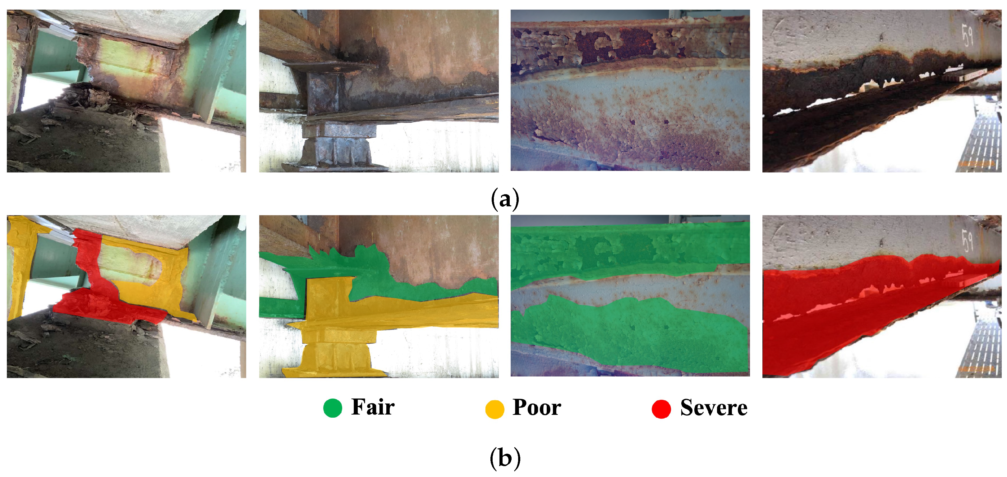
Four sample images and their corresponding annotations are shown in Figure 1. The “Fair”, “Poor”, and “Severe” classes in the annotated images are shown with green, yellow, and red colors, respectively. As can be seen in the figure, no annotation is assigned to peeling paint, visible debris, or minimal corrosion. Freckled rust/sporadic corrosion, exposed steel, and surface corrosion are annotated as “Fair”. Deeper corrosion, such as disintegrated portions of sections or pack rust, is annotated as “Poor”, while any corrosion with section loss, holes, or cavities, or multiple perforations, is annotated as “Severe”. The software used for the semantic mask annotations was LabelMe, an open-source annotation tool that enables users to mark objects or regions of interest in images by drawing bounding boxes, polygons, or points and assigning labels to them.
2.2. Instance Segmentation Models
2.2.1. Mask RCNN
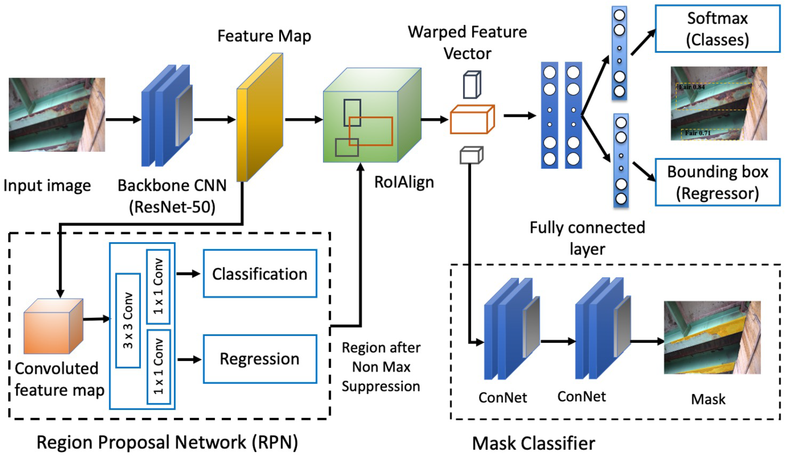
The mask region-based convolutional neural network (Mask RCNN) [19] is a deep learning model designed for instance segmentation tasks. It is an extension of Faster RCNN, which combines object detection and image segmentation by adding a branch for the prediction of object masks. The Mask RCNN backbone is a ResNet-101 architecture that serves as a feature extractor with 101 layers. The early layers detect low-level features, while later layers detect higher-level ones. The feature map in the Mask RCNN architecture retains a spatial abstraction of the input image obtained through convolutional layers. Mask RCNN improves its backbone performance by incorporating a region proposal network (RPN) to find areas containing objects. The regions that the RPN scans over are boxes distributed over the image area called anchors. The final step in the RPN is non-maximum suppression (NMS), which suppresses overlapping object proposals and selects the best ones based on their confidence scores. The remaining object proposals are then passed to the next stage of the Mask RCNN architecture, which performs bounding box regression, classification, and mask prediction. The structure of the Mask RCNN network is shown in Figure 2.
The Mask RCNN loss function is calculated as follows:
where , , and represent classification, regression, and mask loss, respectively. Classification loss measures the discrepancy between the predicted class probabilities and the ground truth class labels for each region proposal and is calculated as
In this equation, is the ground truth label (0 or 1) indicating the true class of the sample, and is the predicted probability of the positive class (object presence) for the sample. Regression loss measures the difference between the predicted bounding box coordinates (e.g., top-left corner, width, height) and the ground truth bounding box coordinates for each region proposal, and it is calculated by
Here, index i represents the specific instance or predicted frame, and is the predicted frame coordinate vector for the i-th instance. is the coordinate vector corresponding to the border of the real area for the i-th instance, and R is the loss function, which computes the element-wise loss between the predicted and target coordinates. Finally, or the mask loss quantifies the dissimilarity between the predicted instance masks and the ground truth masks for each region proposal, and it is defined as
where i iterates over the pixels from 1 to N. The term represents the category label where the pixel is located, and is the probability of the predicted category (). The goal during training is to minimize the total loss value (Equation (1)) as it quantifies how well the model is performing.
Our implementation of Mask RCNN is a library called Detectron2, which is based upon the Mask RCNN benchmark [26]. This library was developed by Facebook AI Research, and it achieved satisfactory results in object detection and segmentation problems. Its implementation is in PyTorch and requires CUDA® due to the heavy computations involved.
2.2.2. YOLOv8
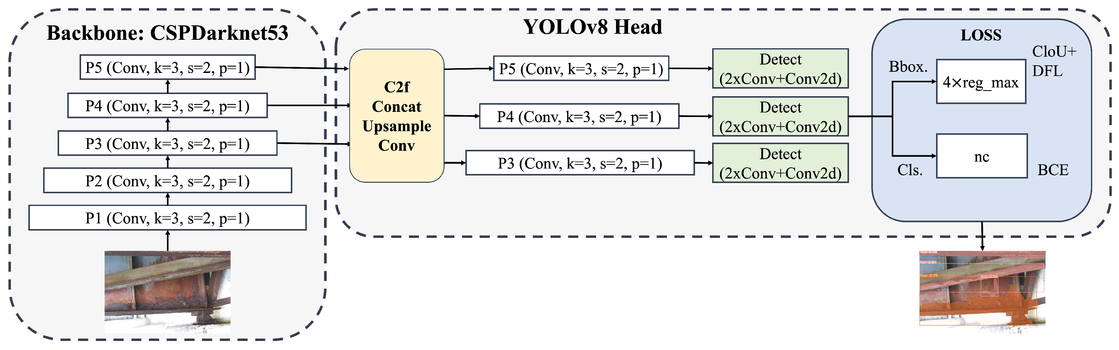
You Only Look Once version 8 (YOLOv8) is the newest state-of-the-art YOLO model that can be used for object detection, image classification, and instance segmentation tasks. YOLOv8 introduces a new backbone network, CSPDarknet53, which consists of 53 convolutional layers and employs cross-stage partial connections to improve the information flow between the different layers [27]. The head of YOLOv8 consists of multiple convolutional layers followed by a series of fully connected layers. YOLOv8 uses an anchor-free model with a decoupled head to independently perform objectness, classification, and regression tasks. This design allows each branch to focus on its task and improves the model’s overall accuracy. YOLOv8 provides a semantic segmentation model called the YOLOv8-Seg model. YOLOv8 segmentation models are pretrained on the COCO dataset. These weights serve as a starting point for the training of any custom dataset. The structure of the YOLOv8 network is shown in Figure 3. One of the key features of YOLOv8 is the use of a self-attention mechanism in the head of the network. This mechanism allows the model to focus on different parts of the image and adjust the importance of different features based on their relevance to the task. Another important feature of YOLOv8 is its ability to perform multi-scale object detection. The model utilizes a feature pyramid network to detect objects of different sizes and scales within an image. This feature pyramid network consists of multiple layers that detect objects at different scales, allowing the model to detect large and small objects within an image.
YOLOv8 uses the complete intersection over union (CIoU) loss [28] and distribution focal loss (DFL) [29] functions for bounding box loss and binary cross-entropy (BCE) for classification loss. Bounding box loss (box_loss) measures the error in the predicted bounding box coordinates and dimensions compared to the ground truth. Segmentation loss (seg_loss) measures the discrepancy between the predicted segmentation masks and the ground truth masks. It encourages the model to generate accurate and precise segmentation masks that align with the ground truth annotations. Classification loss (cls_loss) measures the error in the predicted class probabilities for each object in the image compared to the ground truth. Distribution focal loss (dfl_loss) is a new addition to the YOLO architecture in YOLOv8. DFL loss considers the problem of class imbalance while training a neural network. Class imbalance occurs when one class occurs too frequently and another occurs less frequently. DFL solves this problem by placing more importance on less frequent classes. The overall loss value is typically a weighted sum of these individual losses.
Both the Mask RCNN and YOLOv8 models have demonstrated promising results in various segmentation tasks. Mask RCNN is a two-stage instance segmentation model that combines object detection and pixel-level segmentation. It first generates region proposals using a CNN and then refines these proposals by predicting the class label and generating a mask for each object instance. Mask RCNN is known for its accuracy in segmenting objects with precise boundaries. On the other hand, YOLOv8 is a one-stage object detection model that directly predicts bounding boxes and class labels for objects in an image. It divides the input image into a grid and assigns each grid cell responsibility for predicting objects. YOLOv8 is known for its real-time performance and efficiency.
3. Model Training and Validation
In this study, YOLOv8m-seg, which is a medium-sized segmentation model with over 27 million parameters, was used. The annotated files, which were in .json format originally, needed to be converted to .txt format for the training of the YOLOv8 model. For this conversion, the “json2yolo” github repository was utilized [30]. The training and validation images were randomly selected in each dataset following a ratio of 80% for training and 20% for validation and testing. A total of 412 images were considered for training, 90 images for validation, and 12 images were randomly selected to test the model’s performance. The same training, validation, and testing images were used to train both the YOLOv8 and Mask RCNN models for comparison purposes.
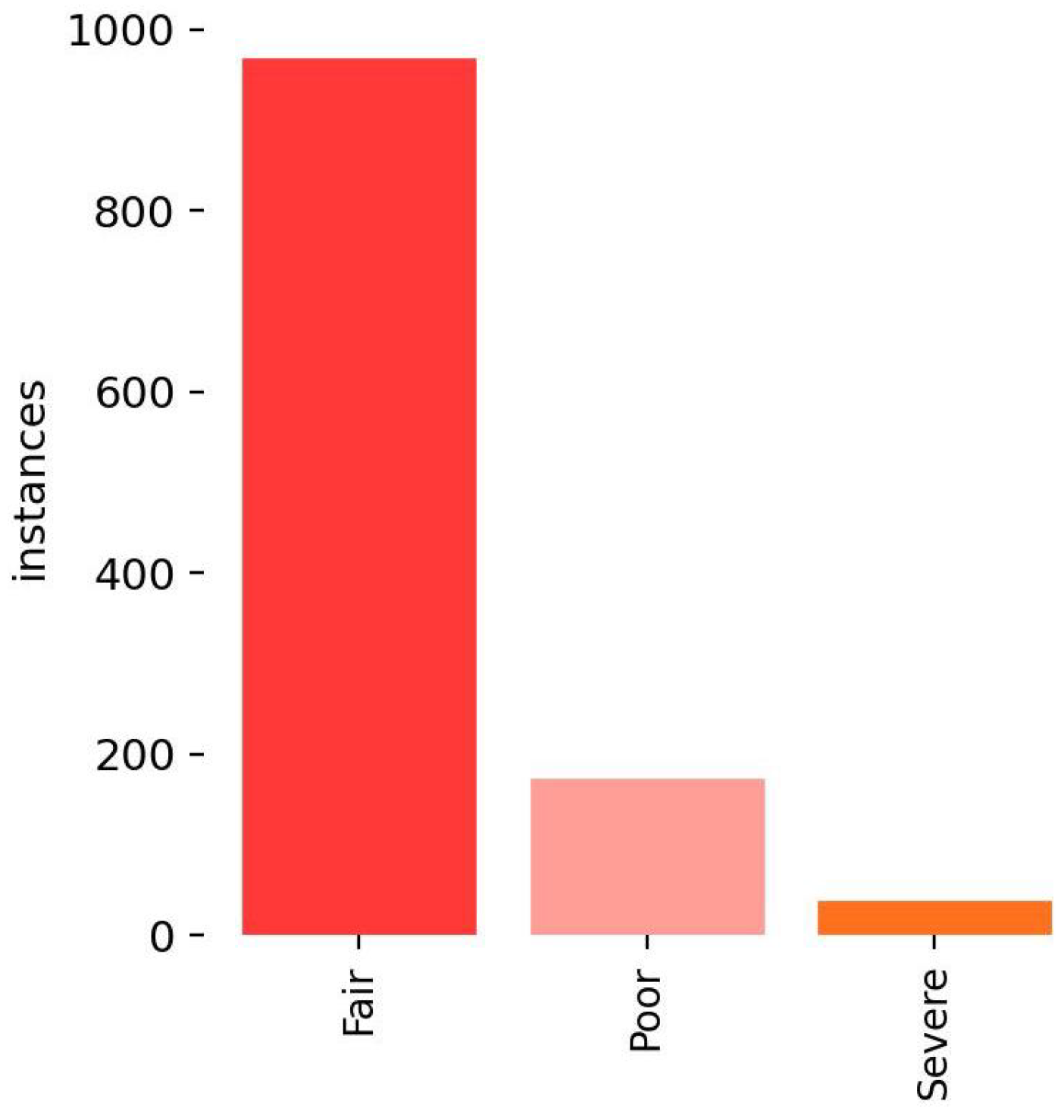
The distribution of instances for each class is depicted in Figure 4. As can be seen in the figure, the number of “Fair” instances is significantly higher than that of “Poor” and “Severe” cases. This observation can be attributed to the relative ease of identifying “Fair” corrosion in the structural elements of the bridge. While most of the collected images contain mild corrosion, it is more challenging to find deeper and more severe corrosion in real bridges.
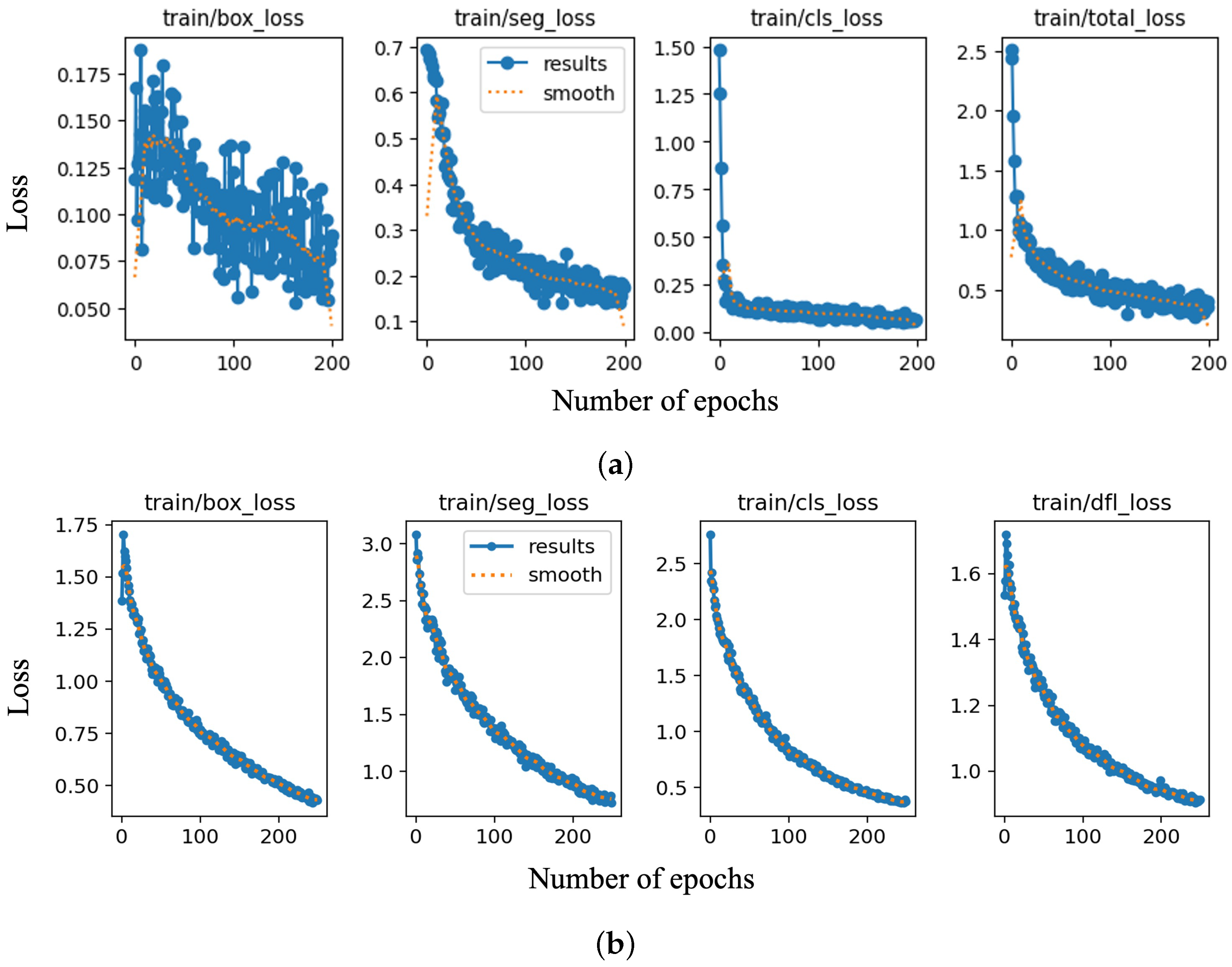
In order to perform the training task, Google Colab Pro was employed, taking advantage of a T4 GPU, the Python programming language, and the large RAM resources. Hyperparameters such as the learning rate, batch size, and number of epochs were optimized based on the performance of the models during training and validation. For the YOLOv8 model, a learning rate of 0.0001 was obtained, along with a batch size of 8 and 250 epochs. The image size was set to 640 by 640 pixels. These values were determined through trial and error to find the optimal balance between model accuracy and training efficiency. Similarly, for the Mask RCNN model, a learning rate of 0.00025 was chosen, along with a batch size of 8 and 200 epochs. The image size was also set to 640 by 640. These values also were selected based on experimentation and previous knowledge of the model’s performance. After training was completed, a file containing the custom-trained weights was saved in the training path. These weights were adjusted during the optimization process to minimize the difference between the predicted outputs and the actual outputs (labels) in the training data. The final weight values were utilized to perform predictions on the selected set of images (test images). This process involved using the trained model to classify and rate the condition of corrosion within the given images. The training loss values versus the number of epochs for the Mask RCNN and YOLOv8 models are shown in Figure 5a and b, respectively. The overall trend of the loss plot shows a consistent decrease, which indicates that the training model is learning and improving its performance over time. The validation loss values versus the number of epochs are also shown in Figure 6.
As can be seen in Figure 5, all types of loss converge to a low and stable value, indicating that both models have learned the patterns in the data. In the case of Mask RCNN, the segmentation loss has a higher value compared to the bounding and classification loss, which suggests that the model struggles with the segmentation tasks. The YOLOv8 trained model has higher segmentation and DFL loss, which shows the inherent difficulty in accurately predicting object masks. The higher DFL loss may indicate that the model is struggling with the class imbalance.
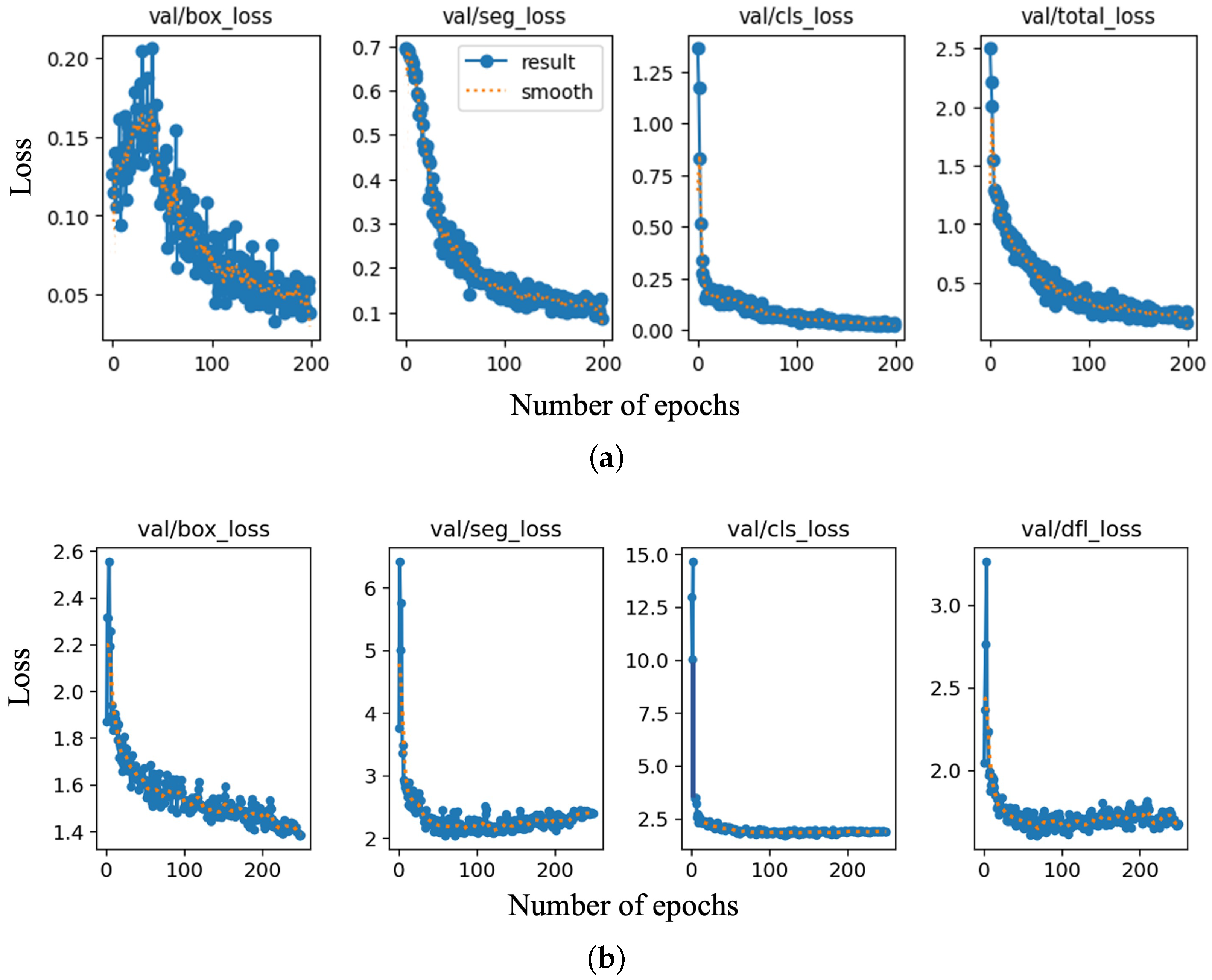
Validation loss measures the model’s performance on a validation dataset, and it provides an indication of how well the model generalizes to unseen data. It was used to tune the hyperparameters, such as the learning rate, number of epochs, batch size, etc. Overfitting (when the training loss continues to decrease, but the validation loss starts to increase) and underfitting (when both the training and validation loss are high) can be avoided by comparing the validation and training loss. The validation loss of the Mask RCNN trained model is as low as its training losses (Figure 6). YOLOv8 shows higher validation loss values compared to the training losses. This could be an indication of overfitting or a lack of diversity in the training dataset.
4. Evaluation
Precision and recall values are two important metrics used to assess the performance of classification models. The precision value quantifies the accuracy of the corrosion detection algorithm, indicating the proportion of correctly identified corrosion instances. The recall value represents the fraction of all target corrosion instances that are successfully detected. The precision and recall values are obtained as follows:
True positive (TP) represents the number of cases that are positive and detected as positive (correctly detected corrosion). False positive (FP) represents the number of cases that are negative but detected as positive (falsely detected non-corrosion). False negative (FN) represents the number of cases that are positive but detected as negative (missed corrosion). Finally, true negative (TN) is the number of negative instances correctly predicted as negative (correctly detected non-corrosion).
The F1 Score combines the precision and recall of a classifier into a single metric by taking their harmonic mean as follows:
Mean average precision (mAP) measures the accuracy of object localization and segmentation by considering the precision and recall values at different levels of intersection over union (IoU) thresholds. It evaluates how well the predicted bounding boxes or segmentation masks align with the ground truth annotations:
where N is the number of classes or categories and is the average precision (AP) for class i. In terms of evaluation metrics for bounding box regression, intersection over union (IoU) is the most popular metric. The IoU for the bounding box and mask can be obtained as follows:
In Equation (9), (B) and (M) distinguish the metrics of segmentation. and represent the prediction and ground truth, while (B) and (M) evaluate the detection (Box) and segmentation (Mask), respectively. mAP50 represents the average precision when the IoU threshold is set to 0.5. This threshold considers a detection as a true positive if the IoU between the predicted and the ground truth mask is greater than or equal to 0.5. This metric provides a more comprehensive evaluation of the models’ performance on the validation and testing datasets. These values for both the YOLOv8 and Mask RCNN trained models were calculated and are listed in Table 2.
The F1 score values in Table 2 show that YOLOv8 achieved an F1 score of 0.730, while Mask RCNN achieved a slightly higher F1 score of 0.745. This indicates that both models exhibit reasonable overall performance, with Mask RCNN having a slight advantage in terms of F1 score and striking a better balance between precision and recall. YOLOv8 achieved higher precision (0.853) compared to Mask RCNN (0.625). This indicates that YOLOv8 tends to make fewer false positive predictions. The Mask RCNN trained model had a higher recall rate (0.922) compared to YOLOv8 (0.647), which indicates its better ability to detect and include relevant objects in its predictions. The mAP50 values of the Mask RCNN trained model were 0.483 on the validation dataset and 0.674 on the test dataset. The YOLOv8 model achieved mAP50 values of 0.484 on the validation dataset and 0.726 on the test dataset. The Mask RCNN model had slightly lower mAP50 values compared to YOLOv8, indicating that YOLOv8 performs better in terms of mean average precision at the 50% IoU threshold. The YOLOv8 model outperformed the Mask RCNN model in terms of speed, with an inference time of 0.03 s per image, compared to 0.12 s per image for Mask RCNN. Based on the available metrics in the chart, the Mask RCNN model generally outperforms the YOLOv8 model in terms of F1 score and recall but YOLOv8 achieves higher precision and mAP50. This implies that YOLOv8 tends to provide more accurate predictions concerning the relevant objects that it detects, albeit with potentially fewer true positives. It is important to note that the comparison is limited to the provided metrics, and further analysis, including additional metrics and experimental conditions, is needed to discuss the performance of these models accurately.
5. Test Results and Discussion
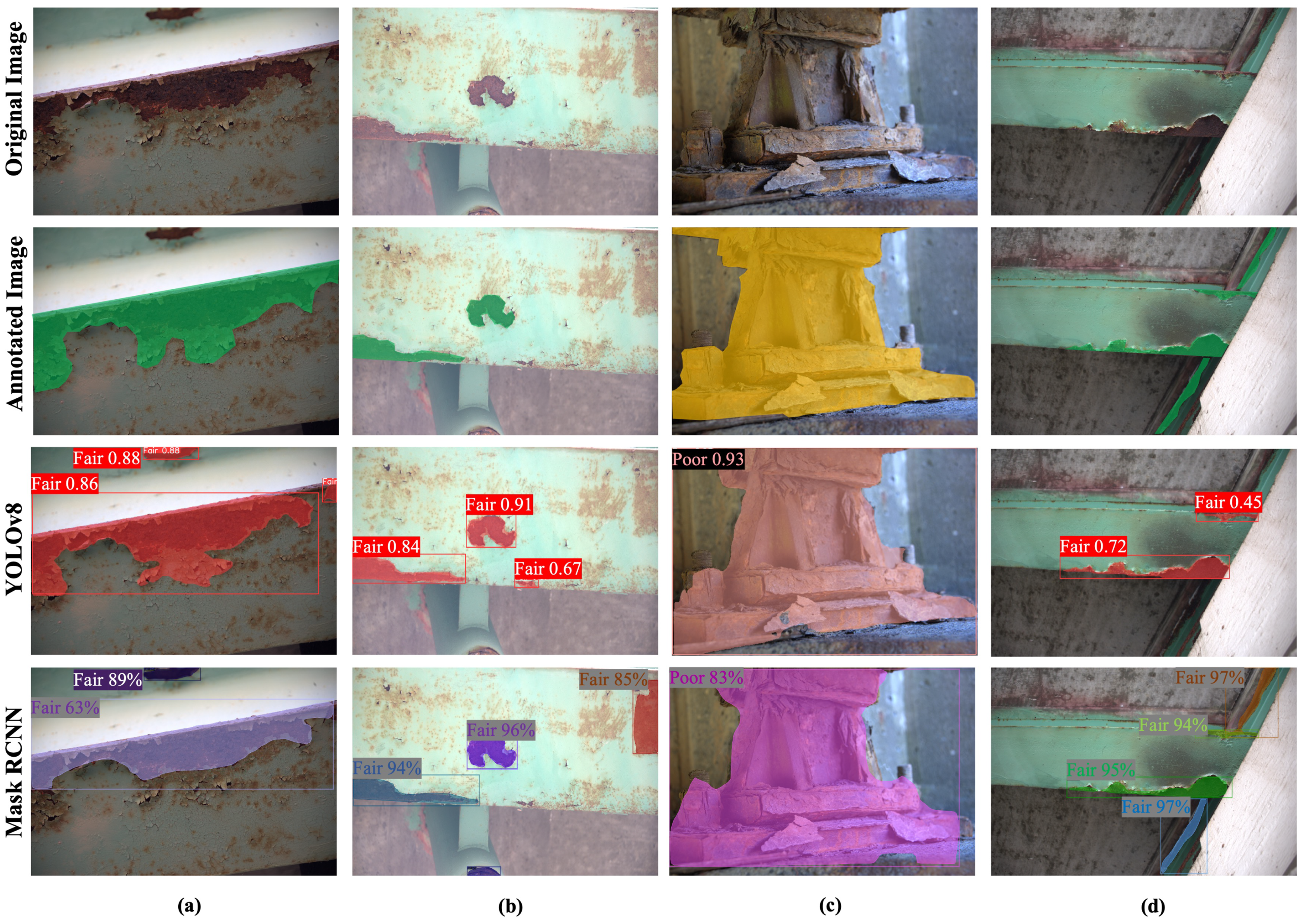
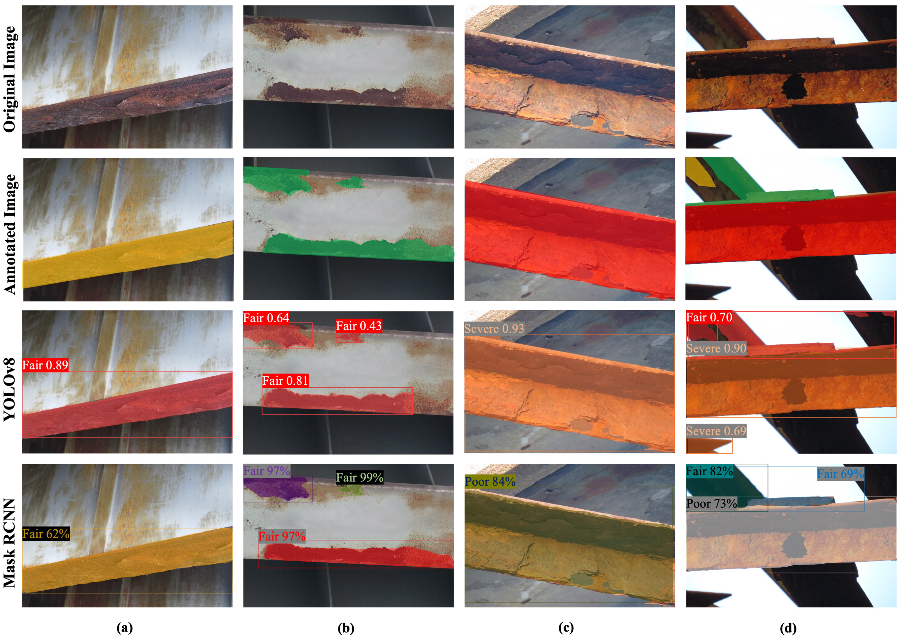
To evaluate the performance of the trained Mask RCNN and YOLOv8 models for corrosion segmentation and condition rating, prediction was performed on the test images that were not used for training and validation. Only objects identified with confidence of 0.5 and 0.35 or higher for Mask RCNN and YOLOv8, respectively, were considered in the test. The representative results are shown in Figure 7, Figure 8 and Figure 9. Each figure contains four images in a row. The first row shows the original test images, the second row represents the corresponding annotations, the third row shows the prediction of the YOLOv8 trained model, and the last row depicts the prediction of Mask RCNN. A brief discussion of the results for each sample image is provided below.
Figure 7a shows mild corrosion in the bottom flange of a beam. The corroded portion of the flange is annotated as “Fair” and its mask is shown in the second row of Figure 7a with a green color. As can be seen in the third and fourth rows of Figure 7a, both the Mask RCNN and YOLOv8 models classified and segmented the corroded portions of the beam correctly. YOLOv8’s mask area and shape is closer to the annotation and has higher confidence compared to Mask RCNN. A small corroded area in the middle of the upper side of the image is correctly detected as “Fair” and segmented by both models, but it is not considered in the annotation due to its small area.
Similar to Figure 7a, Figure 7b contains some “Fair” corrosion. There is a perfect match between the annotation and output of the YOLOv8 model. YOLOv8 also labeled a small area as “Fair”, which is not labeled in the annotation. Mask RCNN labeled two additional instances in the image as “Fair” that are not included in the annotation.
The third picture from the left (Figure 7c) shows a corroded support with relatively severe corrosion, which was annotated as “Poor”. Both of the trained models correctly labeled the corroded area as “Poor”, while Mask RCNN labeled it with lower confidence compared to YOLOv8 (83% vs. 93%). There is some mismatch between the mask depicted by the Mask RCNN trained model and the annotation. It incorrectly detected a small portion of the concrete below the support as poor corrosion.
In Figure 7d, Mask RCNN correctly labels the entire corroded area with higher confidence compared to YOLOv8. Two corrosion instances are missing in the prediction of the YOLOv8 model, while the Mask RCNN trained model correctly classified and labeled all of them with a high confidence score (93% and 97%).
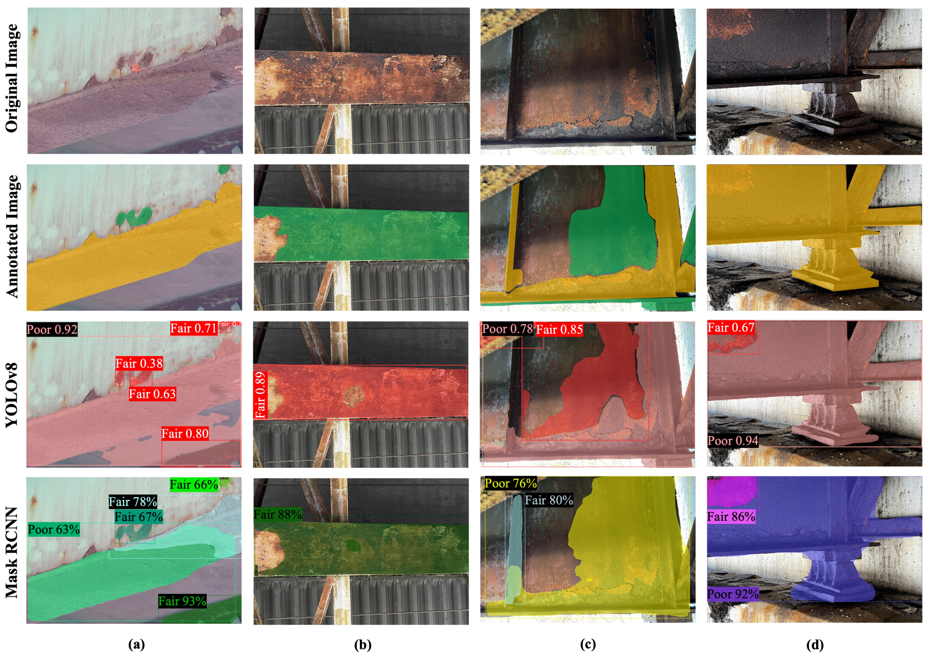
Figure 8a shows a girder flange. The lower part of the beam flange, which was annotated as “Poor”, is correctly labeled and segmented by the YOLOv8 trained model. Some parts of the deck concrete are labeled as “Poor” by YOLOv8, which is not correct. In the lower right corner of the image, a corroded portion of an adjacent girder can be seen, which is not included in the annotation, but both models labeled it as “Fair”. Mask RCNN labeled some parts of the flange as “Poor” and the rest as “Fair”, which is not correct.
As illustrated in Figure 8b, the corroded portion of the lower flange is correctly detected and labeled by both of the models. YOLOv8 has slightly higher confidence compared to Mask RCNN. A small part in the middle of the flange, which seems less corroded compared to the rest of the flange, is excluded from the mask provided by YOLOv8.
YOLOv8 segmented and labeled the web and the upper part of the support, the flange, and the brace as “Poor”, while, in the annotation, only the girder web is considered “Poor” (Figure 8c). The middle part of the web that is less corroded is annotated as “Fair”, while Mask RCNN labeled the entire web and flange as “Poor”. The support and some parts of the brace are excluded from the mask depicted by the Mask RCNN trained model.
As shown in Figure 8d, the corroded support, beam flange, web, and braces are precisely detected by the YOLOv8 trained model. The dark background between the brace and the web stiffener is not included in the YOLOv8-predicted mask, while Mask RCNN detected it as “Poor” corrosion. Moreover, some small parts of the background concrete are included in the mask depicted by the Mask RCNN trained model. A small corroded area in the girder web is labeled as “Fair” by both models, which appears as less severe corrosion compared to the other parts.
Figure 9a shows the bottom flange of a girder, which is delaminated due to corrosion. This corroded area is annotated as “Poor”, but YOLOv8 and Mask RCNN labeled it as “Fair” with confidence of 89% and 62%, respectively. Both models provided a very precise mask of the corroded area since it is easily distinguishable from the background in this image.
As shown in Figure 9b, YOLOv8 was able to detect all instances that were annotated as “Fair”, with a small mismatch in the detected mask. Both the YOLOv8 and Mask RCNN models correctly labeled the corroded parts of the girder flange. The corrosion mask provided by Mask RCNN is closer to the annotation, and it has higher confidence compared to YOLOv8.
Figure 9c illustrates a severely corroded beam with section loss, which was annotated as “Severe”. The YOLOv8 trained model provided a precise mask of the severely corroded beam and labeled it correctly with high confidence (93%). A small part of the background concrete is also included in the mask. Mask RCNN mislabeled the severely corroded brace as “Poor” with confidence of 84%. A small portion of the beam is missing from the mask provided by Mask RCNN.
Figure 9d shows a severely corroded beam with section loss. The dark background of the image was not included in the annotation. The YOLOv8 trained model labeled the severely corroded area of the beam correctly with high confidence (90%). The model labeled a small portion of the dark background as “Severe”, even though this area was not included in the annotation due to its invisible degree of corrosion. Similar to the previous image, the trained Mask RCNN model mislabeled the severely corroded area of the beam as “Poor” with confidence of 73%.
Analyzing the evaluation metric values on the validation and test data, as well as the predictions of the two trained algorithms on the test data, suggests that the YOLOv8 trained model excels in the precision and mAP50 values, providing accurate predictions in some cases. On the other hand, Mask RCNN demonstrates higher recall, capturing more relevant objects. If precision and the minimization of false positives are prioritized, YOLOv8 may be preferred. If the primary focus is comprehensive detection and recall, Mask RCNN might be the better choice.
6. Conclusions
In this study, 514 corrosion images with various degrees of severity were gathered from bridge structural elements, and pixel-wise annotation was performed on each image. The corroded areas were annotated into three classes: “Fair”, “Poor”, and “Severe”. Our annotation process adhered to the guidelines outlined in the Bridge Inspectors Reference Manual (BIRM) and American Association of State Highway and Transportation Officials (AASHTO) regulations for corrosion condition rating (defect #1000). This annotation at the pixel level ensures that the trained algorithms can be directly applied to the corrosion condition rating process, offering practical application for engineers. The collected corrosion images and corresponding annotations can be found online and offer valuable support in advancing the segmentation models by providing high-quality images and corresponding annotations [25]. Two state-of-the-art segmentation algorithms, YOLOv8 and Mask RCNN, were chosen and trained on the labeled dataset to perform pixel-level corrosion segmentation and condition rating. The training process involved optimizing the hyperparameters to obtain the best weights of convolutional layers for accurate and reliable corrosion severity assessments. The trained Mask RCNN and YOLOv8 models achieved mAP50 values of 0.674 and 0.726 on the test images, which is an indication of the models’ ability to perform semantic segmentation with a reasonable level of overlap with the ground truth annotations (IoU = 50%). These results indicate the efficacy of trained Mask RCNN and YOLOv8 models in segmenting and rating corrosion. The main highlights of this study can be summarized as follows.
- The applicability of these algorithms is broad and extends to various conditions. However, it is important to note that the performance of these methods may be influenced by the quality of images and factors such as the lighting conditions and the complexity of the corrosion patterns. It is advisable to ensure the quality of the images during data acquisition to optimize the performance of these segmentation algorithms.
- In terms of performance, we found that both the Mask RCNN and YOLOv8 models achieved satisfactory results in segmenting and rating corrosion. The YOLOv8 model had slightly higher mAP50 values on the validation (0.484) and test (0.726) datasets compared to Mask RCNN (0.483 and 0.674), indicating more accurate predictions while maintaining a good balance between avoiding false positives and capturing as many true positives as possible.
- Mask RCNN model achieved higher F1 score and recall values, which indicate that the model is adept at identifying most of the relevant instances in the dataset. Mask RCNN excels in providing precise instance segmentation with detailed masks, making it suitable for objects with crucial boundaries.
- Mask RCNN has a two-stage architecture, which can be computationally intensive, impacting the real-time performance. Its training may require more computational resources compared to some single-stage approaches. YOLOv8 is designed for real-time object detection, making it efficient in scenarios where low latency is critical.
- In YOLOv8, the default task is object detection, which involves detecting and localizing objects in an image or video. Semantic segmentation, on the other hand, aims to label every pixel in an image with the corresponding class value. While YOLOv8 can be used for object detection, it is not designed specifically for semantic segmentation. It may face challenges in achieving pixel-level instance segmentation accuracy comparable to algorithms specifically designed for semantic segmentation, such as Mask RCNN. Its performance may be influenced by the sensitivity of certain hyperparameters, requiring careful tuning for optimal results.
In the future, to improve the accuracy of the corrosion condition rating model, we aim to obtain more diverse images with varying corrosion severity levels, lighting, and background conditions. Including a greater number of images depicting severe and poor corrosion instances will help to address the class imbalance problem and enhance the segmentation models’ performance considerably.
Author Contributions
Conceptualization, Z.A. and E.N.L.; methodology, Z.A. and S.J.N.; software, Z.A. and S.J.N.; validation, Z.A. and S.J.N.; formal analysis, S.J.N.; investigation, Z.A.; resources, Z.A.; data curation, Z.A.; writing—original draft preparation, Z.A.; writing—review and editing, Z.A. and E.N.L.; visualization, Z.A. and S.J.N.; supervision, E.N.L.; project administration, E.N.L.; funding acquisition, E.N.L. All authors have read and agreed to the published version of the manuscript.
Funding
Funding for this research was provided by the Transportation Infrastructure Durability Center (TIDC) at the University of Maine under grant 69A3551847101 from the U.S. Department of Transportation’s University Transportation Centers Program.
Data Availability Statement
The data presented in this study are available on request from the corresponding author. The data sources are publicly available and referenced in the study.
Acknowledgments
The authors are grateful to MaineDOT and VHB Consulting Engineers for providing infrastructure inspection images and for their valuable insights throughout this work. In particular, we acknowledge Robert Blunt and Benjamin Foster for their assistance with corrosion classification.
Conflicts of Interest
The authors declare no conflict of interest.
References
- Han, X.; Yang, D.Y.; Frangopol, D.M. Risk-based life-cycle optimization of deteriorating steel bridges: Investigation on the use of novel corrosion resistant steel. Adv. Struct. Eng. 2021, 24, 1668–1686. [Google Scholar] [CrossRef]
- Jiang, F.; Ding, Y.; Song, Y.; Geng, F.; Wang, Z. Automatic pixel-level detection and measurement of corrosion-related damages in dim steel box girders using Fusion-Attention-U-net. J. Civ. Struct. Health Monit. 2023, 13, 199–217. [Google Scholar] [CrossRef]
- Savino, P.; Tondolo, F. Civil infrastructure defect assessment using pixel-wise segmentation based on deep learning. J. Civ. Struct. Health Monit. 2023, 13, 35–48. [Google Scholar] [CrossRef]
- Han, Q.; Zhao, N.; Xu, J. Recognition and location of steel structure surface corrosion based on unmanned aerial vehicle images. J. Civ. Struct. Health Monit. 2021, 11, 1375–1392. [Google Scholar] [CrossRef]
- Ameli, Z.; Aremanda, Y.; Friess, W.A.; Landis, E.N. Impact of UAV hardware options on bridge inspection mission capabilities. Drones 2022, 6, 64. [Google Scholar] [CrossRef]
- Feroz, S.; Abu Dabous, S. UAV-based Remote Sensing Applications for Bridge Condition Assessment. Remote Sens. 2021, 13, 1809. [Google Scholar] [CrossRef]
- Khan, M.A.-M.; Kee, S.-H.; Pathan, A.-S.K.; Nahid, A.-A. Image Processing Techniques for Concrete Crack Detection: A Scientometrics Literature Review. Remote Sens. 2023, 15, 2400. [Google Scholar] [CrossRef]
- Rahman, A.; Wu, Z.Y.; Kalfarisi, R. Semantic deep learning integrated with RGB feature-based rule optimization for facility surface corrosion detection and evaluation. J. Comput. Civ. Eng. 2021, 35, 04021018. [Google Scholar] [CrossRef]
- Khayatazad, M.; De Pue, L.; De Waele, W. Detection of corrosion on steel structures using automated image processing. Dev. Built Environ. 2020, 3, 100022. [Google Scholar] [CrossRef]
- Zhou, Q.; Ding, S.; Feng, Y.; Qing, G.; Hu, J. Corrosion inspection and evaluation of crane metal structure based on UAV vision. Signal Image Video Process. 2022, 16, 1701–1709. [Google Scholar] [CrossRef]
- Seo, H.; Raut, A.D.; Chen, C.; Zhang, C. Multi-Label Classification and Automatic Damage Detection of Masonry Heritage Building through CNN Analysis of Infrared Thermal Imaging. Remote Sens. 2023, 15, 2517. [Google Scholar] [CrossRef]
- Petricca, L.; Moss, T.; Figueroa, G.; Broen, S. Corrosion detection using AI: A comparison of standard computer vision techniques and deep learning model. In Proceedings of the Sixth International Conference on Computer Science, Engineering and Information Technology, Qingdao, China, 29–30 May 2016; Volume 91, p. 99. [Google Scholar]
- Atha, D.J.; Jahanshahi, M.R. Evaluation of deep learning approaches based on convolutional neural networks for corrosion detection. Struct. Health Monit. 2018, 17, 1110–1128. [Google Scholar] [CrossRef]
- Jin Lim, H.; Hwang, S.; Kim, H.; Sohn, H. Steel bridge corrosion inspection with combined vision and thermographic images. Struct. Health Monit. 2021, 20, 3424–3435. [Google Scholar] [CrossRef]
- Ronneberger, O.; Fischer, P.; Brox, T. U-Net: Convolutional Networks for Biomedical Image Segmentation. In Proceedings of the International Conference on Medical Image Computing and Computer-Assisted Intervention (MICCAI), Munich, Germany, 5–9 October 2015. [Google Scholar]
- Chen, L.C.; Papandreou, G.; Kokkinos, I.; Murphy, K.; Yuille, A.L. DeepLab: Semantic image segmentation with deep convolutional nets, atrous convolution, and fully connected CRFs. IEEE Trans. Pattern Anal. Mach. Intell. (TPAMI) 2017, 40, 834–848. [Google Scholar] [CrossRef] [PubMed]
- Zhao, H.; Shi, J.; Qi, X.; Wang, X.; Jia, J. Pyramid scene parsing network. In Proceedings of the IEEE Conference on Computer Vision and Pattern Recognition (CVPR), Honolulu, HI, USA, 21–26 July 2017. [Google Scholar]
- Badrinarayanan, V.; Kendall, A.; Cipolla, R. SegNet: A deep convolutional encoder-decoder architecture for image segmentation. IEEE Trans. Pattern Anal. Mach. Intell. (TPAMI) 2017, 39, 2481–2495. [Google Scholar] [CrossRef] [PubMed]
- He, K.; Gkioxari, G.; Dollár, P.; Girshick, R. Mask R-CNN. In Proceedings of the IEEE International Conference on Computer Vision, Venice, Italy, 22–29 October 2017; pp. 2961–2969. [Google Scholar]
- Ta, Q.B.; Huynh, T.C.; Pham, Q.Q.; Kim, J.T. Corroded Bolt Identification Using Mask Region-Based Deep Learning Trained on Synthesized Data. Sensors 2022, 22, 3340. [Google Scholar] [CrossRef] [PubMed]
- Nash, W.; Drummond, T.; Birbilis, N. Quantity beats quality for semantic segmentation of corrosion in images. arXiv 2018, arXiv:1807.03138. [Google Scholar]
- Ryan, T.W.; Mann, J.E.; Chill, Z.M.; Ott, B.T. Bridge Inspector’s Reference Manual (BIRM), Federal Highway Administration, National Highway Institute (HNHI-10), Report No.: FHWA NHI 12-050, 20 February. Available online: https://www.dot.state.mn.us/bridge/pdf/insp/birm/birmchapt0-cover.pdf (accessed on 1 December 2023).
- AASHTO. Manual for Bridge Element Inspection; American Association of State Highway and Transportation Officials: Washington, DC, USA, 2019. [Google Scholar]
- Munawar, H.S.; Ullah, F.; Shahzad, D.; Heravi, A.; Qayyum, S.; Akram, J. Civil infrastructure damage and corrosion detection: An application of machine learning. Buildings 2022, 12, 156. [Google Scholar] [CrossRef]
- Ameli, Z.; Lanis, E.N. Corrosion Condition Rating Database. 2023. Available online: https://digitalcommons.library.umaine.edu/student_work/30/ (accessed on 26 July 2023).
- Facebook AI Research (FAIR). Detectron2: Next Generation Object Detection with PyTorch. 2023. Available online: https://github.com/facebookresearch/detectron2 (accessed on 15 June 2023).
- Terven, J.; Cordova-Esparza, D. A comprehensive review of YOLO: From YOLOv1 to YOLOv8 and beyond. arXiv 2023, arXiv:2304.00501. [Google Scholar]
- Zheng, Z.; Wang, P.; Liu, W.; Li, J.; Ye, R.; Ren, D. Distance-IoU loss: Faster and better learning for bounding box regression. In Proceedings of the AAAI Conference on Artificial Intelligence, New York, NY, USA, 7–12 February 2020; Volume 34, pp. 12993–13000. [Google Scholar]
- Li, X.; Wang, W.; Wu, L.; Chen, S.; Hu, X.; Li, J.; Tang, J.; Yang, J. Generalized focal loss: Learning qualified and distributed bounding boxes for dense object detection. Adv. Neural Inf. Process. Syst. 2020, 33, 21002–21012. [Google Scholar]
- Jocher, G. ultralytics/COCO2YOLO: Improvements. Zenodo. 2019. Available online: https://zenodo.org/record/2738322 (accessed on 1 August 2023).
Figure 1.
(a) Sample images and (b) corresponding annotations.

Figure 2.
Structure of Mask RCNN.

Figure 3.
Structure of the YOLOv8.

Figure 4.
Number of instances for each class: “Fair”, “Poor”, and “Severe”.

Figure 5.
(a) Mask RCNN: bounding box, segmentation, classification, and total loss. (b) YOLOv8: bounding box, segmentation, classification, and distribution focal loss for the training dataset.
Figure 5.
(a) Mask RCNN: bounding box, segmentation, classification, and total loss. (b) YOLOv8: bounding box, segmentation, classification, and distribution focal loss for the training dataset.

Figure 6.
(a) Mask RCNN: bounding box (box_loss), segmentation (seg_loss), classification (cls_loss), and total loss. (b) YOLOv8: bounding box, segmentation, classification, and distribution focal loss (dfl_loss) for the validation dataset.
Figure 6.
(a) Mask RCNN: bounding box (box_loss), segmentation (seg_loss), classification (cls_loss), and total loss. (b) YOLOv8: bounding box, segmentation, classification, and distribution focal loss (dfl_loss) for the validation dataset.

Figure 7.
(a) Bottom flange of a steel beam (b) bottom flange of a main girder (c) Girder support (d) bottom flange of a cross girder.
Figure 7.
(a) Bottom flange of a steel beam (b) bottom flange of a main girder (c) Girder support (d) bottom flange of a cross girder.

Figure 8.
(a) A girder flange and its cover plate (b) bottom flange of a beam (c) girder web (d) girder web, support and bracing.
Figure 8.
(a) A girder flange and its cover plate (b) bottom flange of a beam (c) girder web (d) girder web, support and bracing.

Figure 9.
(a) Bottom flange of a girder (b) bottom flange of a beam (c) lateral bracing (d) top lateral strut.
Figure 9.
(a) Bottom flange of a girder (b) bottom flange of a beam (c) lateral bracing (d) top lateral strut.


Table 1.
Corrosion condition states (AASHTO).
| Condition State | Defect Description in Steel Members |
|---|---|
| “Good” | None |
| “Fair” | Corrosion of the steel has initiated |
| “Poor” | Section loss is evident or pack rust is present but does not warrant structural review |
| “Severe” | The condition warrants a structural review to determine the effect on the strength or serviceability of the element or bridge, or a structural review has been completed and the defects impact the strength or serviceability of the element or bridge |
Table 2.
Evaluation metrics for the trained Mask RCNN and YOLOv8 models.
| Trained Model | Dataset | F1 Score | Precision | Recall | mAP50 |
|---|---|---|---|---|---|
| YOLOv8 | Validation | 0.451 | 0.602 | 0.360 | 0.484 |
| Test | 0.730 | 0.853 | 0.647 | 0.726 | |
| Mask RCNN | Validation | 0.519 | 0.428 | 0.660 | 0.483 |
| Test | 0.745 | 0.625 | 0.922 | 0.674 |
Disclaimer/Publisher’s Note: The statements, opinions and data contained in all publications are solely those of the individual author(s) and contributor(s) and not of MDPI and/or the editor(s). MDPI and/or the editor(s) disclaim responsibility for any injury to people or property resulting from any ideas, methods, instructions or products referred to in the content. |
© 2023 by the authors. Licensee MDPI, Basel, Switzerland. This article is an open access article distributed under the terms and conditions of the Creative Commons Attribution (CC BY) license (https://creativecommons.org/licenses/by/4.0/).
Share and Cite
MDPI and ACS Style
Ameli, Z.; Nesheli, S.J.; Landis, E.N. Deep Learning-Based Steel Bridge Corrosion Segmentation and Condition Rating Using Mask RCNN and YOLOv8. Infrastructures 2024, 9, 3. https://doi.org/10.3390/infrastructures9010003
AMA Style
Ameli Z, Nesheli SJ, Landis EN. Deep Learning-Based Steel Bridge Corrosion Segmentation and Condition Rating Using Mask RCNN and YOLOv8. Infrastructures. 2024; 9(1):3. https://doi.org/10.3390/infrastructures9010003
Chicago/Turabian StyleAmeli, Zahra, Shabnam Jafarpoor Nesheli, and Eric N. Landis. 2024. "Deep Learning-Based Steel Bridge Corrosion Segmentation and Condition Rating Using Mask RCNN and YOLOv8" Infrastructures 9, no. 1: 3. https://doi.org/10.3390/infrastructures9010003