
Development of a Network-Level Road Safety Assessment Procedure Based on Human Factors Principles


Department of Civil and Environmental Engineering, University of Florence, 50139 Florence, Italy
*
Author to whom correspondence should be addressed.
Infrastructures 2024, 9(2), 35; https://doi.org/10.3390/infrastructures9020035
Submission received: 8 January 2024
/
Revised: 30 January 2024
/
Accepted: 9 February 2024
/
Published: 16 February 2024
(This article belongs to the Special Issue Road Systems and Engineering)
Abstract
:Road safety is a central issue in the management and development of a road network. Road agencies must try to identify the most dangerous sections of their network and act on them to improve safety. The most used procedure for this purpose is about considering the indicators based on crashes. However, a mature road safety management system must be able to assess the safety of a road section before accidents occur. The European community is moving in this direction with the update of Directive 2008/96/EC (Directive 1936/2019). This paper proposes a new methodology for carrying out a network-wide road safety assessment on rural single-carriageways and two-lane two-way roads. This procedure accounts for the influence of road characteristics on drivers’ perceptions. The methodology has been developed based on the human factors concepts from PIARC, and it includes a series of checklists that guide an inspector in carrying out a visual inspection of single-carriageway roads. The results from the checklist are then processed into an algorithm, and the level of risk in the analyzed section is provided. The objectives of the procedure are (a) to account for the perceptive aspects that are one of the major causes of road accidents, (b) to provide a proactive procedure in line with the requirements of the European Directive, and (c) to provide a useful instrument that can be easily implemented by road agencies and integrated with other analysis procedures. The procedure has been applied and tested on a case study of six different stretches of two-lane, two-way rural highways in Italy, Germany, and Slovenia (about 65 km). The results show a high degree of concordance with a risk classification based on the accident rate, mainly considering high-risk sections. Therefore, the procedure demonstrated its potential to be a useful instrument to be included in network safety assessments. Road agencies should consider the use of this procedure in their network safety analysis and ranking.
1. Introduction
1.1. Network Safety Assessments
Road traffic accidents represent a major public health issue and one of the leading causes of death, injury, and disability all over the world. Approximately 1.35 million people die each year because of road traffic crashes [1]. It is therefore crucial to continuously make all the necessary efforts to improve the safety of our roads. This must be the objective of road administrations and road practitioners.
Examining road safety involves various methods aimed at assessing the safety levels of specific roads or entire networks. These analyses vary in their nature and approach, leading to different methodologies and terminology. For instance, network screening involves statistically analyzing the crashes within specific road segments, entire roads, or networks, considering both the number and characteristics of the accidents. Elvik [2] defines network screenings as the identification of road sections with safety issues—be it an unusually high number of accidents, a prevalence of severe accidents, or a particular accident type. This approach, which is based on occurred accidents, is termed “reactive”.
Contrastingly, a “proactive approach” aims to identify risky spots before accidents happen. Examples include Road Safety Inspections (RSIs). An RSI aims to identify problem features that are not yet apparent from the accident history or to identify new problems introduced by engineering changes or the ways they are used. RSIs typically rely on visual inspections, with outcomes subject to some level of evaluator subjectivity.
The process of analyzing the safety of the road network is the so-called Network Safety Assessment (NSA). The objective of the process is “to identify sites for further investigation and potential treatment” [3] or “to identify sections of the network that should be targeted by more detailed road safety inspections and to prioritize investment according to its potential to deliver network-wide safety improvements” [4]. The identification of the riskiest sections of a road and the classification of all the sections belonging to the road network allow road agencies to prioritize the interventions, choosing the site that has the highest impact on road safety. Nowadays, NSA procedures mainly rely on accident indices, such as the accident frequency, the accident density, and the accident rate [5]. Accident data are an important source of information to improve road safety analysis, but unfortunately, they are sometimes prone to errors or even just missing (e.g., regression to the mean). To overcome this issue, Accidents Prediction Models (or Crash Prediction Models) with Empirical Bayes adjustment were introduced. These models relate crash expectations to specific road features through statistical analyses [6]. However, drawbacks include potential oversight of site-specific details and limited representativeness across countries due to varying factors’ influences [7]. The use of Accidents Prediction Models has proven to be a consistent method for making reliable crash frequency predictions, and thus improve a reliable NSA, but the implementation of an Accidents Prediction Model requires a large amount of data. Those data are not always available, mainly in low- and middle-income countries. Once an Accidents Prediction Model has been defined, this does not ensure that it is suitable for every analysis. Sometimes, it is necessary to adapt existent AMPs to local conditions [8,9].
An interesting proactive approach to an NSA procedure was proposed by Cafiso et al. [10] and considered by Erieba et al. [11]. This approach relies on RSI and provides a safety index suitable for the ranking of the analyzed sections. Moreover, another study from Cafiso et al. [12] demonstrated that RSI, which is carried out following a systematic and structured procedure, produces the same results, even if carried out by different inspectors. Moreover, some drawbacks related to the time required to implement RSIs can be solved using fast procedures and new technologies [13].
Recent years saw the development of new methodologies attempting to combine Accidents Prediction Models’ efficiency with the detailed analysis of standard RSIs. Examples include iRAP methodology [14,15,16], the Australian National Risk Assessment Model “ANRAM” [17], and the method proposed in the “Network Wide Road Safety Assessment—Methodology and Implementation Handbook” [18]. Moreover, among different ways of carrying out road safety analysis at the network levels, some consider the use of new technologies [19,20,21], the use of surrogate safety measures [22,23], or focus more on speed consistency [24].
Finally, it must be noted that the updated European Community directive 2008/96/EC now mandates Network-Wide Road Safety Assessment in member states. It requires a visual examination of road design features and analysis of sections operational for over three years with a high proportion of serious accidents relative to traffic flow [4].
For these reasons, it is crucial to identify assessment indices. Such indices can be qualitative, such as the one identified in [10]. Qualitative indices generally help to identify the main risk level of a section. However, it is difficult to rank different sections within the same risk level and thus give priority to one or the other. For this reason, quantitative indices are also crucial. Such types of indices also allow us to classify the road sections analyzed, as demonstrated in [10,14,16,25,26,27]. Road agencies can plan their intervention based on those indices, identifying the most critical sections of the road and scheduling when and how to intervene.
1.2. Human Factors
It has been proved that most accidents are a consequence of drivers’ behavior [28,29] and that the behavior is strictly related to the road, both to its geometrical elements and its environment [30]. Drivers are the core of the road system. Drivers are humans, and they must not be considered machines. They cannot strictly obey specific geometrical rules nor analyze all aspects of a complex situation in a few seconds in a perfect, mechanical way. For this reason, the concept of human factors (HF) should be applied to road safety. Many studies identify HFs as a key factor in correct road perception and thus in accident occurrence [31]. Some of these studies consider, for example, bend curvature perception [32,33], reaction time and perception of the potentially critical locations [34,35], human workload and decision making [36], road familiarity and influence of experience [37,38], and the influence of road marginal elements on speed and behavior [39,40,41]. Understanding the factors that influence the road–driver relationship, which are the triggering factors of accidents, helps to avoid driver mistakes. A road that does not lead drivers to make mistakes can be defined as a self-explaining road [42]. The basic notion of a self-explaining road, which originated in the Netherlands, is a “traffic environment which elicits safe behavior simply by its design” [43,44]. By this concept, the driver should clearly understand the road they are driving, its elements, and its features, changing their driving behavior according to the road elements. The self-explaining roads concept could appear utopistic; nevertheless, designers should tend to make roads on a human scale.
1.3. Research Objective and Overcoming the Gaps
The main knowledge gap addressed by this research is to translate the already known human factors principles [45,46] into a systematic procedure capable of quantitatively measuring the level of safety of a specific road stretch. This objective also covers the space of the updated Directive 2008/96/EC, which requires a procedure able to visually investigate the road safety level proactively. Moreover, as also highlighted by other authors [47,48], segmentation is still an issue in carrying out NSAs. Different road segmentations may often create different results, with a lack of consistency against different segmentations. This procedure tries to overcome this gap by proposing three different levels of segmentation: a first level with long sections for a fast first screening of the stretch, a second level with short segments for the detailed analysis and evaluation of the stretch, and again a much longer section to group the results of the shorter segments into a more practical segmentation for management for road agencies.
The new procedure allows us to carry out an NSA based on visual inspections, which is based on human factor principles. The procedure has been developed for rural single-carriageway roads. The procedure described in this paper was already introduced in the work of Paliotto et al. [49] and recently finalized [50]. The current version has been strengthened and amended to make it more suitable for its use. Specifically, the version presented in [49] presents some limitations:
- -
- During the first step of the procedure, the evaluation of Potentially Critical Locations (PCLs, see Section 2.2.2) was made without following a systematic procedure and was made only considering all different expectation-related aspects together (i.e., general expectations, punctual expectations, and visibility), with a high possibility of subjective judgments.
- -
- During the second step, the Human Factor Tool from PIARC [51] was used with only a few adjustments for the score calculation.
- -
- The procedure was applied to three road stretches.
The new procedure aims at improving these points by achieving the following:
- -
- Consider a systematic and automated process to ensure an objective and fast first screening of the PCLs. This assures the reduction in time required to analyze all the PCLs in the second step.
- -
- Improve the Human Factor Tool by introducing and modifying some requirements, developing guidelines for its application (achievable in the material attached to the paper), and developing a digital tool (in Excel) to expedite its application.
- -
- Apply the procedure to the already analyzed stretch (for a comparison of the results) and three new stretches.
2. Materials and Methods
The following paragraphs present the steps to follow to carry out the procedure. Please refer to the paragraph “List of acronyms and definition” for the meanings of each acronym.
2.1. Structure of the Procedure
The procedure is divided into three different steps according to the conceptual scheme shown in Figure 1.
The first step (top-down process) allows us to make a first screening of the road to identify the Potentially Critical Locations (PCLs) that have a high possibility of being critical. The PCLs considered [49] are listed in Section 2.2.2. In the first step, the road analyzed is divided into Expectation Sections (EXSEs), which are sections of several km on average. EXSEs are crucial to identify road characteristics that allow us to determine if a PCL is expected or not as clearly explained in Section 2.2.1. In the second step (evaluation process), the Human Factors Evaluation Tool (HFET) is applied to each Human Factors Evaluation Segment (HFES), which are shorter segments of about 300–400 m on average. The third step (bottom-up process) allows us to organize the results so that they are suitable for a network classification (longer sections). This means grouping many HFESs into single Network Assessment Sections (NASs). For each NAS, a risk code RC is calculated. The RC allows us to identify four different levels of risk and to make a ranking of the NAS. The obtained level of risk is calculated without considering accident data. For this reason, the procedure can be considered a full proactive procedure based on visual inspections.
2.2. Step 1 of the Procedure
The main aim of the first step is to identify the characteristics of the roads analyzed while considering their influence on driver expectations. In this step, EXSEs are identified. EXSEs are road sections where the driver has specific similar driving demands, like a curvy section with a similar radius or an interurban section with a logical consistency of design elements and speed. At the same time, the roadside gives the driver a consistent impression that contributes to an overall impression of the road section. So, the driver subconsciously builds up a specific expectation of how the road alignment develops and which driving program is appropriate. PCLs are qualitatively evaluated by judging the level of compliance between possible expectations induced by the road and the real road development and configuration. This is achieved by assigning to each PCL a risk level for the general expectations (GEXs) (three risk levels: high, medium, and low), visibility (VIS) (three risk levels: high, medium, and low), and punctual expectations (PEXs) (two risk level: high and low). The assignment is made while taking care of the following:
- -
- GEX: how the PCL is expected considering the EXSE to which it belongs (e.g., a pedestrian crossing cannot be expected within a forest where no buildings are visible);
- -
- VIS: evaluate if sufficient decision sight distance is present based on the expected speed and alertness that the driver is expected to have while driving that specific EXSE that includes the analyzed PCL (the driver needs more time to see, understand, and react to the pedestrian crossing considered in the previous example);
- -
- PEX: punctual expectations generated by the specific configuration of the road and the field of view close to the PCL; they are evaluated through fast visual inspection of the road by human factors experts. Contrary to GEX and VIS, which can be calculated, PEX is derived from the qualitative judgments of inspectors. For this reason, only two levels of risk are considered for PEX, which means: “some main issues are present” (high risk level) or “no or very low issues are present” (low risk level).
2.2.1. Identification of PCLs and EXSEs
The steps to follow for the identification of PCLs and EXSEs are the same as defined in Paliotto et al. [49]. PCLs are any area where drivers must adapt their driving program by changing speed, braking, steering, or changing lanes. Normally, they are junctions, intersections, stops of public transport, exits, driveways, curves, carriageway width reductions, or pedestrian/cyclist crossings. PCLs are directly identified by driving through the road, considering the road database, looking at the design documents, or satellite images. An example of PCL identification is provided in Figure 2.
EXSEs are road sections characterized by the same expectations for the driver. Thus, driving performances are related to driver expectations about the road and their consistency with real road development. EXSEs are defined based on the section’s main characteristics, which are the road category, the road winding, and the road perception of possible interaction (PPI).
The broad category includes motorway, rural highway, rural local, urban arterial, urban connectors, and urban local. This paper focuses on the application of the procedure only related to rural highways.
Road winding is defined based on the value of the curvature change rate (CCR), following Equation (1).
where the following apply:
- CCR = curvature change rate [gon/km];
- γi = angular change of the geometric element “i” [gon];
- Li = length of the geometric element “i” [km];
- n = number of geometric elements of the road section (tangents, circular curves, spirals) [-].
For rural highways, three levels of road windings have been identified based on the value of the CCR.
- High winding: CCR > 350 gon/km;
- Medium winding: 350 gon/km > CCR > 160 gon/km;
- Low winding: CCR < 160 gon/km.
The PPI represents how much the driver expects interactions with other crossing-road users. Two levels of PPI (details on how those levels are calculated can be found in [50] together with some examples) are defined for rural highways: low and medium.
- Low level: only rural areas can be considered at a low level. A low level means very few or no perceived possible interactions. The surrounding environment is almost natural, without any trace of anthropization, if not the road itself.
- Medium level: this level represents the upper level of rural areas. Such PPI is often representative of suburban areas, where the density of houses and commercial activities is reduced. Medium level can also address rural road stretches that pass through small villages or groups of houses along the road or which pass through an area with many driveways and at-grade intersections due to the presence of many activities and factories.
A different EXSE starts when there is a change in the winding level or PPI level. The consistency of each PCL with its EXSE must then be evaluated, as explained in detail in Section 2.2.2. The actual procedure differs from that proposed in the previous work from Paliotto et al. [49] because it considers different risk levels for each aspect analyzed (i.e., GEX, VIS, PEX). An example of EXSEs identification is provided in Figure 3. The value of the computed CCR and the identified level of PPI are shown in the same figure.
Based on the winding level and PPI level, the levels of expected speed (VE) and alertness can be defined. VE is the range of speed the driver is expected to travel at. Alertness defines the level of attention of the driver, and thus, indirectly, it influences the activated level of resources to process information from the environment. High alertness corresponds to high available resources. High alertness translates into a reduced time required to process information and respond to environmental stimuli.
All the different levels of VE and alertness corresponding to different combinations of winding and PPI for rural highways are presented in Table 1. The relationships in Table 1 highlight, for example, that a driver who is driving on a rural highway with a high level of winding and a medium level of PPI is expected to have a high level of alertness and to drive at a relatively moderate speed (50–80 km/h). On the other hand, if a driver is driving on a rural highway with low winding and low PPI, they are not ready to react to any unexpected event (low level of alertness), and their speed is expected to be relatively high (80–100 km/h). At the end of the EXSE identification process, all EXSEs are characterized by a level of winding, a level of PPI, a level of VE, and a level of alertness.
2.2.2. Evaluation of PCLs
PCLs are evaluated considering GEX, VIS, and PEX.
GEX Evaluation
The evaluation for GEX is automatically made considering the criteria in Table 2. Such criteria were derived both considering a literature review of design standards of several countries (Italy, Germany, England, Slovenia, Portugal, Australia, Canada, Austria, Switzerland) and a survey conducted on a sample of about 50 people with a valid driver license of different ages and gender. Detailed data about the design standards and the survey are provided in [50].
In Table 2, it is possible to derive, for example, that a relatively sharp curve (curve20, which requires a speed deceleration of about 20 km/h) is not expected on a section with low curvature and low PPI (thus a high risk). On the opposite, the same curve is expected on a high winding section with medium PPI (thus a low risk). The maximum level of PPI for rural roads is medium (M).
VIS Evaluation
To assess the VIS level, the visibility of the PCL must be checked. The visibility of locations along the road is commonly used in engineering; however, most of the time, the distance checked is the stopping sight distance. For specific locations, many design standards also account for the decision sight distance, for example, [52]. Stopping sight distance is considered an instinctive reaction to facing a sudden problem and avoiding an accident, while the decision sight distance accounts also for the time needed to correctly perceive and plan how to react to a specific situation on the road. PIARC defines a general decision sight distance considering subdividing the space (and time) approaching the PCL into four different sections [46]. From the one closer to the PCL, the sections are the maneuver section (where the braking action is mainly carried out), the response section (2–3 s, mainly necessary to the driver to set the maneuver), the anticipation section (2–3 s, necessary to comprehend the location), and the warning section (4 s, necessary under specific conditions to advise drivers about oncoming location). A well-designed road should have the maneuver, response, and anticipation sections; for this reason, PIARC defines the First Rule of Human Factors (4–6 s rule). Consequently, the assessment of the VIS level considers that optimal conditions are when the PCL is visible from a distance traveled in more than 6 s. This means that the maneuver, response, and anticipation sections are present (assuming that the maneuver section hardly takes more than 2 s; otherwise, it means that a long emergency braking is required, and stopping sight distance must be considered). The traveled distance D2 is calculated considering the higher speed in the range of the VE, multiplied by t2, as defined in (2). The time t2 is considered as 6 s for EXSE with a low alertness, 5 s for EXSE with a medium alertness, and 4 s for EXSE with a high alertness (considering 6 s or less as the “optimal” threshold may appear not precautionary; however, when calculating the distance, the considered speed is the maximum of VE range. This compensates for the choice of a relatively reduced time. It must also be noted that detailed and more precise calculations are possible but are not suggested at this stage because a fast screening is required now to exclude the less dangerous PCLs from a detailed analysis (that is carried out in Step 2)). The higher the alertness of the driver, the less time necessary to perceive and detect the PCL.
where the following apply:
- D2 = threshold distance between the medium and low VIS level [m];
- t2 = 6 for low alertness, 5 for medium alertness, and 4 for high alertness [s].
Table 3 shows the outcome of the calculations for the two VE levels for rural highways. Within that distance, the PCL must be clearly and continuously visible. If the visibility is higher than D2, it can be assumed that the PCL has no visibility problem, and thus the VIS level of risk is low. On the other hand, if the available sight distance is less than D1, a high risk is present concerning VIS. D1 is calculated considering Equation (3). Available sight distance between D2 and D1 leads to a medium risk for VIS.
where the following apply:
- D1 = threshold distance between the medium and high VIS level [m];
- t1 = 4 [s].
PEX Evaluation
PEX levels consider the composition of the road and the road environment, and thus the composition of the field of view and its influence on the right perception of the road. These conditions must be evaluated close to the PCL, starting from about 6–10 s before the PCL. Unfortunately, it is not possible to define objective criteria to calculate the PEX level; thus, this process is up to the inspector. To assess the PEX level of each PCL, the inspector must drive along the road stretch in both directions, trying to figure out if some PEX issues are present. Because of the subjectivity of this evaluation, it has been decided to consider only two levels of PEX: low risk and high risk. A low risk level means that there are not any issues or only a few. High risk means that many issues are present, or a few big issues.
The evaluation should be carried out without a deep analysis. The main aspects to consider are reported in Table 4. The table is divided into three main investigation topics (“density and shape of the field of view”, “elements in the lateral roadside environment support optimal lane keeping”, and “depth of the field of view”) with their relative subsections. The contents of this table represent a sort of checklist for the inspector. Generally, it can be assumed that if inspectors find some issues concerning two out of three of the investigation topics, then the PCL should be classified as a high level of PEX. However, this is not a rule; the inspector must try to understand if the found issues are relevant. For this reason, to carry out the assessment, the inspector must be trained in human factors.
PCL evaluation is not mandatory. However, this first screening of PCLs is highly recommended to ensure that only the locations with the higher possibility of being dangerous are analyzed in step 2 with the Human Factors Evaluation Tool (HFET). The detailed analysis of all the PCLs with the HFET would require more time than the fast evaluation of the PCLs described in Step 1.
2.3. Step 2 of the Procedure
In the second step, the detailed analysis of the road is carried out and the Human Factors Evaluation Tool (HFET) is applied to the Human Factors Evaluation Segments (HFESs). The HFESs are segments composed of one or more challenging location (CHL) and their relative challenging transition (CHTs). The updated version of the HFET allows us to analyze at the same time all the CHLs belonging to the same HFES. The HFET is available together with the guidelines for its application in the Supplementary Materials of this paper (GUIDELINE for the application of the HUMAN FACTORS EVALUATION TOOL). The second step is divided into three main sub-steps:
- Identification of CHLs;
- Identification of CHTs and HFES;
- Application of the HFET.
2.3.1. Identification of CHLs
CHLs are PCLs that are not clearly perceived by the driver because of some problems concerning VIS, GEXs, and/or PEXs. The consequence is that the driver does not change his driving program or tries to change it too late, causing hazardous maneuvers. A PCL is promoted to CHL when at least one risk level related to expectations (VIS, GEX, or PEX) is high and one is medium. This concept is clarified in Table 5, where all the possible combinations of VIS, GEX, and PEX levels are presented, together with the outcome of each combination.
A PCL could be CHL only for one direction of travel. For this reason, in the analysis, the direction in which the location is challenging must be specified.
2.3.2. Identification of Challenging Transitions (CHTs) and Human Factors Evaluation Segments (HFESs)
Once the CHLs have been identified, the area to evaluate with the HFET must be chosen. This area is the road stretch preceding and including the CHL, and it is called challenging transition (CHT). CHTs typically start 10–12 s before the CHLs and can include other elements of the road that are not CHLs or even other CHLs. If the latter is the case, the two overlapping CHTs (one for each CHL) must be merged, creating a single CHT. This final CHT is then called the Human Factors Evaluation Segment (HFES) because this is the segment that is evaluated with the HFET.
The scheme in Figure 4 summarizes the three steps required. CHLS and CHTs must be considered first in one direction and then in the other direction because, based on the direction of travel, they can change. Consequently, HFESs are also different for each direction.
As said before, the typical length of a single CHT is the distance traveled in 10–12 s [46] in addition to the length of the CHL itself. The speed required to calculate the distance can be considered as the maximum speed in the EXSE’s VE range, reduced by 10 km/h, as shown in (4).
where the following apply:
- DCHT = distance traveled in 10–12 s [m];
- t3 = 10–12 [s].
Table 6 shows the calculated distances for the two different VE levels. Nevertheless, those distances do not need to be exact; they must be used as references. Inspectors may decide to reduce or increase those distances if the operating speed seems to be very different than the speed considered in (4). Distances less than 150 or higher than 300 m are discouraged.
Figure 5 shows an example of two CHLs with their CHT from road SR2 in Tuscany (red line). One CHL is represented by a pedestrian crossing (yellow); the other CHL is represented by a curve (green). The two CHTs are overlapping; thus, they are merged to create a single CHT, HFES (purple). The HFES in the example of Figure 5 is about 450 m long.
2.3.3. Application of the Human Factors Evaluation Tool (HFET)
The HFET is provided by three different sheets, each of them representing one of the rules of human factors. The tool should be applied following the guidelines for its application provided in the documentation attached to this paper.
The results provide the Human Factors Score (HFS), a numerical index that ranges between 0% and 100% and which assumes the following significance: HFS < 40% (highlights a high-risk HFES, 40% ≤ HFS ≤ 60% is medium risk, and HFS > 60% is low risk. The HFS is provided for each of the three rules of human factors [46] and considers all the rules together (Total HFS).
2.4. Step 3 of the Procedure
The third step is needed to group the results obtained from the analysis of HFESs. Longer sections are more useful while implementing a Network-wide Road Safety Assessment because they can be more easily represented and because road administrations often prefer to intervene on longer road stretches [16]. These sections are called Network Assessment Sections (NASs). Moreover, the results obtained from the second step of the procedure for each HFES must be unified in a single result that is representative of the NAS. For these reasons, the third step of the procedure concerns the following:
- Identification of NASs;
- Calculation of the Risk Code (RC) to assign to each NAS.
2.4.1. Identification of NASs
NASs are road stretches taken as a reference by road agencies. The results of the entire procedure are provided for each NAS, and the results allow us to rank each NAS, allowing the road agency to define its intervention priority. The scope of the NASs is thus related to the scope of the road agency. For this reason, road agencies may choose the length of the NASs based on their requirements. Different segmentation criteria can be used by road agencies. A very common one is to consider sections with the same traffic level. Other criteria can be to have sections of a fixed length that can be easily compared (because of their same length) and that can also be easily associated with the km posts. Another possibility to have a specific length for each NAS is because some other evaluations have been made that have a specific segmentation length, and the road agency wants to compare the results of this procedure with the results of some others. All these possibilities are made possible because of the flexibility, at this step, in the choice of NAS’s length. However, some limitations should be considered to account for the road category and its characteristics. On non-motorway roads, NASs with a length higher than 5 km are discouraged because the road can greatly differ within 5 km. Moreover, if the road is quite complex with a changing environment, lengths of a maximum of 2 km are suggested. Finally, it is recommended to divide the network into NASs of the same length as possible. However, while determining the NASs, each HFES should be wholly included in a NAS, and thus an exact length is not always assured. In two-lane, two-way rural highways, a length of 1 km is suggested [53]. Such a length is long enough to be applied on the network, but it is still quite short to provide sufficiently focused results. An example of NAS identification is provided in Figure 6.
After NASs have been identified, all the road stretches that belong to NAS but do not belong to HFESs are classified as Inconspicuous Segments (INCSs). INCSs are considered segments with a HFS of 100%.
2.4.2. Calculation of the Risk Code (RC)
Focusing on the objectives of the new procedure [4], the code to assign to each NAS must allow for the identification of at least three safety levels and should allow for a ranking of the NAS. Therefore, each NAS is defined by an alphanumerical code that is divided into three parts, as shown by Figure 7: a first part composed of a letter and a number, a second part composed of a number, and a third part composed of two numbers.
The first term identifies the safety level of the NAS. The second term gives a numerical value that represents the most critical HFES within the NAS. The last term is instead a measure of the variance of the results within the same NAS. It allows us to understand if, within the same NAS, a single critical area is present, but the remaining part of the NAS is in good condition (or the opposite). The alphanumerical values in Figure 7 have the following meanings:
- A = letter representing the worst level of HFS present, including the HFS for each rule and the Total HFS (R = red, at least one score < 0.40 within the rules; Y = yellow, no red scores, and at least one score < 0.60 within the rules; G = green, all other results), for both directions;
- B = The number of results of level “A” (see before), considering the worst results of the HFSs for each rule and the Total HFS (min = 0, max = 4);
- C = The worst total result within the NAS;
- D = Weighted Average of the Total HFS and length of each HFES and INCS;
- E = Standard Deviations of the Total HFS of each HFES and INCS, considering the segment length.
The RC refers to both directions considered together. The ranking of the NASs follows a two-level ranking.
The first ranking identifies the risk level of the NAS, and thus it is based into four groups:
- Very high risk: “AB” part of the code is equal to “R4”;
- High risk: “AB” part of the code is equal to “R2” or “R3”;
- Medium risk: “AB” part of the code is equal to “R1” or “Y4”;
- Low risk: all the remaining cases.
These four risk levels are consistent with the number of different risk levels required by the new European Directive [4].
High and very high levels both mean a high probability of accident occurrence, while medium and low risk can be associated with a low risk of accident.
The second level ranking considers instead a ranking within the same risk level. This second ranking is made following the criteria presented in Table 7. It must be considered that each parameter composing the code follows the order in which they are presented (AB-C-D/E). This means that considering the same results of part “A” of the code, priority is given to the NAS, which has a higher part “B”. Generally, parts D and E of the code are not necessary for the ranking. However, they provide important information about the composition of the NAS, which can help the road agency in the following stage of intervention. At the end of step 3, the ranking is obtained for all the NASs belonging to the road network.
2.5. Validation of the Procedure
The procedure has been validated by comparing the results obtained from its application to six road stretches of rural two-lane two-way roads, with an accident index considered for the same roads. The accident index considered is the accident rate (AR), which is the number of accidents per vehicle kilometer traveled in one year. Three different safety levels, which are based on the AR results, have been considered. Finally, a comparison has been made between both the safety level results and the ranking obtained by the two indices (AR and RC), respectively, utilizing the Freeman–Halton extension of Fisher’s test because of the low number of variables considered and utilizing Kendall’s coefficient of concordance (W). Fisher’s test [54] is used for categorical data that result from classifying objects in two different ways; it is used to examine the significance of the association between the two kinds of classification (thus a 2 × 2 contingency table) that is used to calculate exactly the significance of the deviation from a null hypothesis (e.g., p-value). The Freeman–Halton extension of the test [55] allows for the extension of the test to contingency tables greater than 2 × 2. In this research, a 3 × 3 contingency table has been used. Kendall’s W (also known as Kendall’s coefficient of concordance) is a non-parametric statistic for rank correlation [56]. The coefficient is a measure of the agreement between several judges who have rank-ordered a set of entities. Kendall’s W ranges from 0 (no agreement) to 1 (complete agreement).
2.6. Repeatability
The considered procedure is mainly based on a visual inspection of the road that is carried out in step 2 of the procedure while applying the HFET. While applying the HFET, the inspector is asked to judge some different aspects and characteristics of the road and its environment, and this may lead to possible differences in judgments if different inspectors carry out the analysis. A clear guideline for the application of the HFET, with clear criteria for judgments, is expected to greatly reduce the differences in judgments. To test the repeatability of the procedure, in 2022, another team of inspectors have been asked to analyze the same stretch of road SR2. The results are discussed in Section 2.7.
Calculation of the AR and AR levels
The AR performance measure has been chosen as the most representative for a comparison. Indeed, AR is a safety performance that quantifies the safety of a single vehicle driving along a road stretch. As defined in Equation (5), the AR for a road segment is defined as the number of accidents in the analysis period (i.e., accident frequency) divided by the number of vehicles that pass through that segment in the same period (in million vehicles) and divided by the length of the segment.
where the following apply:
- AR = accident rate [accidents/(km × Mvehicles)];
- n = number of accidents in the analysis period [accidents];
- L = segment length [km];
- AADT = average annual daily traffic value in the analysis period [vehicles/day].
To define the risk level based on AR, it has been decided to follow the procedure proposed by Miar [53], which developed upon the proposal from Norden et al. [57]. Two thresholds have been identified: ARmax and ARmin. The risk levels are assigned as follows:
- ARi < ARmin = low risk level;
- ARmin < ARi < ARmax = medium risk level;
- ARi > ARmax = high risk level.
ARi is the accident rate for section “i”, calculated following Equation (5). ARmin and ARmax can be calculated following Equations (6) and (7).
where the following apply:
- K = constant of Poisson probability distribution function, taken as 1.282 (confidence interval of 90%) [58];
- ARm = the average accident rate of the analyzed site (e.g., road stretch) calculated with Equation (8).
- Mi = the exposure momentum calculated with (9) for section “i”.
- np = total number of accidents that occurred in the considered period “p”;
- t = total number of sections in the analyzed site;
- Li = length of the “i” section;
- AADTi,p = average annual daily traffic of section “i” in the whole considered period “p” (sum of the AADTi of each year).
2.7. Consistency
The procedure allows road administrations to choose the most suitable segmentation for NAS. To test the consistency against different segmentation of NASs, the two stretches of road SR2 and road B38 have been analyzed considering three different NAS segmentations: 1 km, 2 km, and based on traffic changes.
2.8. Test Roads
The road stretches considered for the validation of the procedures are two-lane, two-way rural roads, both primary and secondary roads. A total of about 65 km of roads have been considered. Because of the objective of being an international procedure, the stretches considered are from two Italian roads, three German roads, and one Slovenian road.
The two roads from Italy are the roads SR2 and SR206. SR2 and SR206 are two rural highways located in the center of Italy, which differ from each other for both geometrical and functional characteristics. The road SR2 stretch ranges from km 280.600 to km 292.400 (11.8 km total) in a hilly environment with many curves and few short tangents. The road SR206 stretch ranges from km 27.800 to km 42.400 (14.6 km total) in a plain terrain with many long tangents and few curves. The traffic database has been provided by the Tuscany Region. The analysis period considered for traffic is 2014–2018. The accident database was provided by ISTAT (Istituto Nazionale di Statistica).
The German stretches considered are from Road B38, road L3106, and road L3408. The stretch of road B38 analyzed ranges between km 1.200 after Section 6118-001 and Section 6118-036. The road develops through a plain and hilly terrain. The radii used are quite high, and the operating speeds are high (between 80 km/h and 100 km/h). The road L3106 stretch analyzed runs from Section 6218-045 to Section 6118-005 for a total length of about 7.5 km. The road develops through a hilly terrain and maintains a soft, curvy track. The road L3408 analyzed starts 1.600 km after Section 6418-217 and ends 0.4 km before Section 6418-207, for a total length of about 3.0 km. The road characteristics are similar to those of the road L3106. Geometrical, traffic, and accident data for the German roads have been provided by Hessen Mobil. For all the stretches, the accidents database refers to the period 2018–2020.
The Slovenian Road 106 stretch develops from the southern part of Ljubljana for about 16 km. The road stretch analyzed corresponds to Section 261. Road 106 is an important road that connects the capital, Ljubljana, with the southern part of the country. Thus, many vehicles of different types travel the road. From km post 3.200 to km post 5.200, the carriageway cross-section is composed of a 2 + 1 lane, with a double lane in the south direction. The road is mainly a fast road, developing first in plain terrain and then in hilly terrain. Traffic data have been provided as a single data set for each year in the period 2015–2019. The accident database has been provided by the Slovenian Infrastructure Agency and refers to the period 2015–2020.
Figure 8 shows the satellite images of each road stretch. The images are of different scales and are mainly provided to understand the geometry of the roads and the environment they pass through.
3. Results
3.1. Main Results
After the RC was calculated for each NAS, the AR was calculated for each NAS. Table 8 shows the list of identified NASs, the road they belong to, their length, their average AADT, the obtained RC with the consequent risk levels and ranking, and the AR for each NAS with the consequent risk levels and ranking. The results are ordered from the worst section to the best one, considering the RC.
The outcomes from the statistical analysis are as follows:
- Freeman–Halton extension of Fisher’s test: p-value significance of 0.004 < 0.05; thus, the null hypothesis that the variables assume these risk levels by chance can be rejected;
- Kendall’W of 0.78, with a p-value of 0.001 < 0.05; thus, the null hypothesis that the variables assume this ranking by chance can be rejected.
All the statistics confirm a good correspondence, and the null hypothesis can be rejected for all the statistics. Moreover, it is possible to build the contingency table for risk level comparison, which is shown in Table 9. The greater the values on the matrix diagonal, the better the correspondence between the two classifications. In the table, it can be observed that there is a very good correspondence between the medium levels and a good correspondence between the high levels. In the same table, the NASs classified as low or medium risk for both indices are colored in green. These NASs can be considered “sections that do not require interventions”. On the opposite, risky sections (“sections that require interventions”) are colored in red.
Considering the sum of numbers in the diagonal divided by the total number of NASs, the overall concordance is 56%. The results show that a better correspondence is present considering the high risk level. It must also be noted that only in one NAS, the difference among the results is of “two levels”, which means that the section is classified as high risk for one index and as low risk for the other. In all other cases, if the risk level is not the same, it is the immediately preceding one (or immediately following one). Indeed, while considering only the “section that requires interventions”, which are the high-risk level sections (red cells), and the “section that does not require interventions”, which are the low- and medium-risk sections (green cells), the correspondence is 81%. Finally, a regression analysis of RC values vs. AR has been performed to test the existence of a numerical correlation. Because RC is a qualitative variable, it has been translated into numbers considering the different combinations of the first part of the RC as a number, following the criteria in Table 10. The scale used is linear, and the difference between each different RC has been set to 1. The relationship between AR and the associated value of the RC is plotted in Figure 9. The results show a low correlation when all the NASs are considered. However, some interesting distribution of the results can be observed. The most varying results are linked to the value “5”, corresponding to RC = R1. Such RC means that one of the rules presents some major problems that need attention, but the other aspects are quite good. Such RC identifies a medium risk level. Because of the structure of the procedure that gives more weight to the worst situation, such results can be expected as collateral drawbacks because, in the R1 sections, it is possible to expect a high variance of accidents: the critical issue identified may cause some accidents, but if many other aspects are good, it is possible to also expect a small number of accidents. This confirms that the procedure can identify critical locations and locations that are not critical at all, but it is not very precise at the intermediate level. However, it is generally the same considering accident-based performance measures because the intermediate level is much more sensitive to accident variations over the different years of the analyzed period. So, it can be stated that in this higher variance around RC = R1, the two measures are in some way concordant.
Finally, considering the possible variation of accidents over the years (that is a common issue considering accident statistics), it has been decided to test a linear correlation by making an average of the AR values of the NAS having the same RC. The correlation that was obtained is very good (r = 0.86; R2 = 0.7391). The results are shown in Figure 10. This confirms the overall good prediction of the procedure. Nevertheless, additional analysis and evaluations (larger dataset) are suggested before defining a numerical relationship between the two variables.
3.2. Repeatability
The repeatability of the procedure has been investigated by the application of the procedure on road SR2 by another team. The result, which is shown in Table 11, demonstrates that even if applied by different inspectors, the proposed procedure leads to very similar results. Minor differences are present in the length of the sections, which derive from the difference in the definition of the CHLs and CHTs, and minor differences are present in the RC. This also creates little difference in the ranking. However, the most interesting thing is that the risk level is the same for each NAS, the number of NASs is the same, and the two critical sections are the same (the two sections classified as “high” or “very high” risk). These results are very encouraging, even if additional teams should apply the procedure on different roads.
3.3. Consistency
The consistency of the procedure has been investigated, considering the possibility of different segmentation. Segmentation is a crucial task in road safety analysis, as highlighted by Cafiso et al. [47]. Two different segmentations are proposed in addition to those considered during the test of the procedure (1 km segmentation): a fixed length of 2 km and a variable length based on traffic changes. This new application was made both on road SR2 and road B38 stretches. Figure 11 and Figure 12 show the RC and the characteristics of the road SR2 and road B38 NASs obtained considering a segmentation of 1 km, 2 km, and a segmentation based on traffic characteristics (when the AADT changes, another segment is defined). Dark red indicates a very high-risk section, red indicates a high-risk section, yellow indicates a medium-risk section, and green indicates a low-risk section. In the traffic-based segmentation, HFESs containing intersections where a change in traffic is present have been included wholly within the same NAS; thus, for a very short segment close to the intersection, the traffic of the NAS assumes a different value. It must be noted that a segmentation based on traffic must be made only when traffic data are reliable.
Looking at the results, the following considerations can be made.
- NAS length is related to the HFESs. Sometimes, it is not easy to define short sections (e.g., 1 km), and sometimes, it is not easy to define longer sections (e.g., 2 km). For this reason, the results should be consistent, even if NASs sometimes have a length that differs much from the reference one.
- When a lack of traffic data is present or when traffic is constant for a long stretch, NAS defined, considering traffic, may become very long, missing much of its significance. This is the case of road SR2. In this case, even if traffic is chosen as a reference for NAS segmentation, it is suggested to consider a maximum section length (2 km is suggested).
- It has been confirmed that longer NASs are likely classified as riskier than shorter NASs because they may include more “red results” (high risk) from the HFESs. However, the choice of considering the most critical results within the section to provide the RC for the section has been made during the development of the procedure to ensure that the presence of high-risk HFESs is never hidden. This is very important; otherwise, some risky sections could be underestimated.
4. Discussions and Conclusions
The main purpose of this work was to develop and validate an innovative network-wide road safety assessment procedure based on human factors. Moreover, based on the requirements of the European Directive [4], the procedure should include visual inspections of the road, it should be a proactive procedure, and it should provide at least three levels of risk. All these requirements have been achieved. The procedure allows the identification of risky road sections of the network and can apply to rural two-lane, two-way roads. This research demonstrates the importance and influence of human factors in road safety.
The procedure has been validated by comparing the results to accident data (i.e., accident rate). The results are good overall. The main strengths and realizations of this work can be summarized as follows:
- This research provides a validated instrument that analyzes the road using human factors. Such an instrument is innovative and highly required because most accidents occur because of human errors induced by the road.
- It has been found that it has a high capacity to identify dangerous locations. The comparison with accident-based analysis shows a good statistical correspondence between the results. An average of 56% of NASs were considered with the same risk level for both analyses. Considering only two levels, sections that require intervention (high risk) and sections that do not require intervention (low and medium risk), the concordance rises to 81%. Overall, statistical analysis also demonstrates that such concordance is significant.
- This procedure overcomes many of the segmentation issues that always burden road safety analysis. Those issues are very common in standard RSI analysis and accident-based analysis. This has been performed while considering different segmentations for different types of analysis (step 1, step 2, and step 3 of the procedure). In steps 1 and 2, the segmentation is linked to the specific issues that need to be analyzed, while in step 3, the segmentation is made while considering the most efficient way for road agencies to use the results on a network level.
- It is a proactive procedure because accident data are not required. Thus, it can be applied to those road stretches for which no accident data are available or when accident data are not reliable.
- It provides information about the specific risks of the road, aiding in the decision of possible interventions (in step 2, it provides a detailed analysis of the issues of the segment).
- It does not need much data, and the data needed can be easily found.
- It allows the definition of intervention priority. The calculated RC allows the identification of four levels of risk and the order of the NAS within those levels from the most critical to the least critical.
- It proves to be repeatable and easy to implement after short training courses. This has been proven by the application of the procedure from a different inspection team that was trained in human factors principles. The training course was a two-day course.
However, together with many achievements, some limitations are also present. The identified limitations are hence listed.
- Despite an overall good concordance between the results, some sections show differences in the evaluation. Thus, a detailed analysis of those sections must be carried out with detailed inspections and/or the accidents of the successive years monitored.
- Identifying EXSEs is a crucial task. The application of the procedure from a different inspection team shows that when longer sections of the road are considered, the PPI level can be ambiguous. Different evaluations of PPI are reflected in the evaluation of PCLs, both concerning GEXs and VISs. However, if an EXSE is judged as “medium” PPI instead of “low”, but the winding level is the same, the risk of missing information is moderate, and medium-level CHLs are likely missed. On the opposite, if the PPI is judged as “low” instead of “medium”, no information is missed, but more CHLs are identified with some additional computing time while applying the HFET.
- Subjective judgments of PEX. Even if references and short checklists have been provided to evaluate PEXs, the judgments are still subjective; thus, different results in the evaluation may occur. However, the procedure shows that those differences are few. Moreover, the choice of giving greater importance to the most critical result for evaluating HFESs and NASs allows for the reduction in error of PEX judgments in step 1. That is because very critical locations for PEX are likely identified by all inspectors. The main difference in the evaluations is related to locations around the “medium level” because they can be ambiguous, and the inspector cannot be sure if they must be selected or not.
- Limited sample for the study. Despite the overall good results, additional tests should be made considering additional road stretches and additional inspector groups.
- The procedure must be tested strongly against the inspector’s subjective judgments. Also, in this case, this research provides a first important step in that direction, but to be sure about the reliability and repeatability of the procedure, more inspectors should apply it to the same road (and also to others), and the results of the judgments should be compared.
- The procedure is consistent against different NAS segmentations when considering the capacity to identify the most critical section of the road. On the other hand, when very long sections are considered, the probability of section risk overestimation increases, thus reducing the consistency of the overall judgment. For these reasons, a maximum length of 2 km is suggested. This measure should be validated in subsequent experiments.
- It must be remembered that this procedure focuses on the identification of road stretches that are prone to cause accidents. Thus, it identifies those points of the road where an accident can likely occur. It does not consider the consequence of an accident; hence, it does not consider the severity of an accident. For this reason, to have a comprehensive analysis of all the safety aspects of the road, this procedure should be complementary to some others that can identify how severe the possible outcome could be.
- The procedure does not account for the influence of traffic; thus, it cannot provide an index of risk accounting for the number of vehicles traveling along the stretch. However, this is only a partial limitation. The proposed procedure has been developed to analyze the safety level of a road without considering traffic exposure. The results from the procedure identify the risk of a single vehicle driving along the road to incur an accident because road-induced driver behavior does not comply with the road characteristics. This value of risk is fixed for a specific road stretch based on its characteristics.
- The resources necessary to carry out the procedure on a network range. The application of the procedure requires time and trained inspectors. Fast analyses that consider only observed accidents are easier to implement.
A comparison has also been made considering the achievements of Paliotto et al. [50] and the actual achievements. In Section 1.3 of the Introduction, some limitations of the previous work have been highlighted, and the objective of this new research is listed. After the application of the procedure, it can be stated that the main objectives have been reached. The procedure can now be applied systematically, reducing the subjectivity of different inspectors to a great extent. The process has been expedited overall, and its application has been simplified. Moreover, the outcomes from the two versions of the procedure have been compared, and they highlight once more the robustness of the procedure: only minor changes in segmentation and results have been observed, which have minor influences on the risk level of the section. A comparison of the 10 more critical sections among roads SR2, B38, and 106 (the road analyzed in this research and in [49]) is presented in Table 12. The results are quite the same, with only NAS 4 from road B38 changing its level of risk from medium to high.
To conclude, the authors think that road agencies should consider the use of this procedure for their network safety analysis and ranking and not be discouraged by the apparent difficulty of its application. Road safety must become the priority of road agencies, together with road functionality. A safe road design must always consider that the main users of the road are drivers, and thus the road must be designed around them and for them, accounting for all their limitations and qualities.
Supplementary Materials
Author Contributions
Conceptualization, A.P.; methodology, A.P.; software, A.P.; validation, A.P., and M.M.; formal analysis, M.M.; investigation, A.P. and M.M.; resources, A.P. and M.M.; data curation, A.P. and M.M.; writing—original draft preparation, A.P.; writing—review and editing, A.P. and M.M.; visualization, A.P.; supervision, M.M.; project administration, A.P.; funding acquisition, M.M. All authors have read and agreed to the published version of the manuscript.
Funding
This research received no external funding.
Data Availability Statement
The original contributions presented in the study are included in the article/Supplementary Material; further inquiries can be directed to the corresponding author/s.
Acknowledgments
We thank the Regione Toscana administration, Hessen Mobil, and the Slovenian Government, who provided information about the roads. We thank J.S. Bald and L. Domenichini for their assistance, insight, and expertise that greatly assisted the research. We also thank the second inspection team composed of P. Di Michele and J.M. Lanuza. Finally, a great thank you and credit goes to S. Birth, a road psychologist who was a pioneer in the application of human factors in road safety.
Conflicts of Interest
The authors declare no conflicts of interest.
List of Acronyms and Definitions
The acronyms and terms that have been used to address specific concepts raised in the development of the procedure are listed. In addition, the following terms are used with these related meanings:
- Segment: a part of a road of short length (generally within 1 km), which is part of a section;
- Section: a part of a road of medium length (generally more than 1 km), which is part of a stretch;
- Stretch: a part of a road that spans several km.
| Term | Meaning |
| AADT | Annual Average Daily Traffic. |
| AR | Accident rate. |
| CHL | Challenging Location. CHLs are PCLs that are not clearly perceived by the driver, because of some problems concerning VIS, GEXs, and/or PEXs. The consequence is that the driver does not change his driving program, or tries to change it too late, causing hazardous maneuvers. |
| CHT | Challenging transition. This is the area preceding and including the CHL. |
| EXSE | Expectation Section. A road section where the driver has specific similar driving demands, like a curvy section with similar radii, or an interurban section with a logical consistency to its design elements and speed. At the same time, the roadside gives the driver a consistent impression that contributes to their overall impression of the road section. So, the driver will build up, subconsciously, a specific expectation of how the road alignment will develop and which driving program is appropriate. |
| GEX | General Expectations. Expectations the driver has about the road, derived from previous experience: both life experience (e.g., road type) and “last km” experience (based on the characteristics of the last km of the road traveled). |
| HFES | Human Factors Evaluation Segment. An HFES is composed of a sequence of consecutive and/or overlapping challenging transitions that are merged. |
| HFET | Human Factors Evaluation Tool. This allows us to evaluate the compliance of the road characteristics to the human factor demand. |
| HFS | Human Factors Score. The result, in percentage, of the application of the Human Factors Evaluation Tool. It is called the HFS both in the results of the First, Second, and Third Rule and the Sum of all the Rules. |
| INCS | Inconspicuous Segment. Part of a road section that is easy to drive and without any obvious design deficiencies or human factors deficiencies. It does not have to be evaluated with the Human Factors Evaluation Tool. |
| NAS | Network Assessment Section. This section is considered to provide the result of the procedure. The whole analyzed network will be divided into many NASs. NASs will be the element to which the road agency will refer to decide where to intervene. NASs may include many HFESs. |
| NSA | Network safety assessment. |
| PCL | Potentially critical location. Any area where drivers must adapt their driving program by changing their speed, braking, steering, or changing lanes. Normally they are junctions, intersections, stops for public transport, exits, driveways, curves, carriageway-width reductions, or pedestrian/cyclist crossings. |
| PEX | Punctual expectation. Expectations the driver has about the road, derived from the surrounding location: the punctual road image (and the Gestalt) creates specific expectations about the specific location. |
| PPI | Perception of possible interaction. This is a quantification of how the road layout shows possibilities for interactions with other road users (e.g., the presence of intersections, accesses, and pedestrian crossings). |
| RC | Risk code, which summarizes the outcomes of the application of the procedure for each NAS. |
| RSIs | Road safety inspections. |
| VE | Expected speed has been introduced to provide a range of possible speeds for an EXSE. Based on the EXSE’s characteristics it is expected that drivers traveling the EXSE will hold a speed within the range of the VE. |
| VIS | Visibility. When the VIS term is used, it means the available sight distance between the driver and the PCL, which allows the driver to see, perceive, and understand the PCL. |
References
- WHO. Global Status Report on Road Safety 2018. 2019. Available online: https://www.who.int/publications/i/item/9789241565684 (accessed on 7 January 2024).
- Elvik, R. Assessment and Applicability of Road Safety Management Evaluation Tools: Current Practice and State-of-the-Art in Europe; TØI Report 1113/2010; Institute of Transportation Economics, Norwegian Centre for Transport Research: Oslo, Norway, 2010; ISBN 978-82-480-1171-2. [Google Scholar]
- FHWA-SA-16-038; Reliability of Safety Management Methods Diagnosis. U.S. Department of Transportation: Washington, DC, USA, 2016.
- European Parliament and European Council, Directive 2008/96/CE of the European Parliament and of the Council of 19 November 2008 on road infrastructure safety management, amended by Directive (EU) 2019/1936; European Union: Brussels, Belgium, 2019.
- PIARC. Road Accident Investigation-Guidelines for Road Engineers. pp. 1–51. 2013. Available online: https://www.piarc.org/en/order-library/19593-en-Road (accessed on 7 January 2024).
- AASHTO. Highway Safety Manual, 1st ed.; American Association of State Highway Transportation Professionals: Washington, DC, USA, 2010. [Google Scholar]
- Sacchi, E.; Persaud, B.; Bassani, M. Assessing international transferability of highway safety manual crash prediction algorithm and its components. Transp. Res. Rec. 2012, 2279, 90–98. [Google Scholar] [CrossRef]
- La Torre, F.; Domenichini, L.; Corsi, F.; Fanfani, F. Transferability of the Highway Safety Manual Freeway Model to the Italian Motorway Network. Transp. Res. Rec. J. Transp. Res. Board 2014, 2435, 61–71. [Google Scholar] [CrossRef]
- La Torre, F.; Domenichini, L.; Branzi, V.; Meocci, M.; Paliotto, A.; Tanzi, N. Transferability of the highway safety manual freeway model to EU countries. Accid. Anal. Prev. 2022, 178, 106852. [Google Scholar] [CrossRef]
- Cafiso, S.; La Cava, G.; Montella, A. Safety Index for Evaluation of Two-Lane Rural Highways. Transp. Res. Rec. J. Transp. Res. Board 2007, 2019, 136–145. [Google Scholar] [CrossRef]
- Erieba, O.; Pappalardo, G.; Hassan, A.; Said, D.; Cafiso, S. Assessment of the transferability of European road safety inspection procedures and risk index model to Egypt. Ain. Shams Eng. J. 2024, 15, 102502. [Google Scholar] [CrossRef]
- Cafiso, S.D.; La Cava, G.; Montella, A.; Pappalardo, G. A Procedure to Improve Safety Inspections Effectiveness and Reliability on Rural Two–Lane Highways. Balt. J. Road Bridge Eng. 2006, 1, 143–150. Available online: https://bjrbe-journals.rtu.lv/article/view/1822-427X.2006.3.143%E2%80%93150 (accessed on 7 January 2024).
- Cafiso, S.D.; Kiec, M.; Pappalardo, G. Innovative methods for improving the effectiveness of road safety inspection. In Proceedings of the VI International Symposium of Transport and Communications, New Horizons, Doboj, Bosnia and Herzegovina, 17–18 November 2017. [Google Scholar]
- Derras, A.; Amara, K.; Oulha, R. Application of the IRAP Method Combined with GIS to Improve Road Safety on New Highway Projects in Algeria. Period. Polytech. Transp. Eng. 2022, 50, 414–425. [Google Scholar] [CrossRef]
- 2011. Available online: www.eurorap.org (accessed on 7 January 2024).
- iRAP. iRAP Methodology Fact Sheets–iRAP. Available online: https://irap.org/methodology/ (accessed on 7 January 2024).
- Jurewicz, C.; Steinmetz, L.; Turner, B.; Cammack, M. Australian National Risk Assessment Model, vol. AP-R451-14. Sydney NSW 2000 Australia: Austroads Ltd. Level 9, 287 Elizabeth Street. 2014. Available online: www.austroads.com.au (accessed on 7 January 2024).
- European Commission. Network Wide Road Safety Assessment Methodology and Implementation Handbook; Publications Office of the European Union: Brussels, Belgium, 2023.
- Shah, S.A.R.; Brijs, T.; Ahmad, N.; Pirdavani, A.; Shen, Y.; Basheer, M.A. Road Safety Risk Evaluation Using GIS-Based Data Envelopment Analysis—Artificial Neural Networks Approach. Appl. Sci. 2017, 7, 886. [Google Scholar] [CrossRef]
- De Luca, M. A comparison between prediction power of artificial neural networks and multivariate analysis in road safety management. Transport 2017, 32, 379–385. [Google Scholar] [CrossRef]
- Singh, G.; Pal, M.; Yadav, Y.; Singla, T. Deep neural network-based predictive modeling of road accidents. Neural Comput. Appl. 2020, 32, 12417–12426. [Google Scholar] [CrossRef]
- Aichinger, C.; Nitsche, P.; Stütz, R.; Harnisch, M. Using Low-cost Smartphone Sensor Data for Locating Crash Risk Spots in a Road Network. Transp. Res. Procedia 2016, 14, 2015–2024. [Google Scholar] [CrossRef]
- Hu, Y.; Li, Y.; Yuan, C.; Huang, H. Modeling conflict risk with real-time traffic data for road safety assessment: A copula-based joint approach. Transp. Saf. Environ. 2022, 4, tdac017. [Google Scholar] [CrossRef]
- Llopis-Castelló, D.; Bella, F.; Camacho-Torregrosa, F.J.; García, A. New Consistency Model Based on Inertial Operating Speed Profiles for Road Safety Evaluation. J. Transp. Eng. A Syst. 2018, 144, 04018006. [Google Scholar] [CrossRef]
- Cafiso, S.; Di Graziano, A.; Pappalardo, G. Safety Inspection and Management Tools for Low-Volume Road Network. Transp. Res. Rec. 2015, 2472, 134–141. [Google Scholar] [CrossRef]
- Montella, A.; Mauriello, F. Procedure for ranking unsignalized rural intersections for safety improvement. Transp. Res. Rec. 2012, 2318, 75–82. [Google Scholar] [CrossRef]
- Fancello, G.; Carta, M.; Fadda, P. Road intersections ranking for road safety improvement: Comparative analysis of multi-criteria decision making methods. Transp. Policy 2019, 80, 188–196. [Google Scholar] [CrossRef]
- Treat John, R.; Tumbas, N.S.; McDonald Stephen, T.; Shinar, D.; Hume, R.D.; Mayer, R.E.; Stansifer, R.L.; Castellan, N.J. Tri-Level Study of the Causes of Traffic Accidents: Final Report Volume II: Special Analyses; Indiana University: Bloomington, IN, USA, 1979. [Google Scholar]
- Birth, S.; Demgensky, B.; Sieber, G. Relationship between Human Factors and the Likelihood of Single-Vehicle Crashes on Dutch motorways; Report for Rijkswaterstaat Dienst Verkeer en Scheepvaart: Utrecht, The Netherlands, 2015. [Google Scholar]
- Theeuwes, J. Sampling information from the road environment. In Human Factors for Highway Engineers; Elsevier: Amsterdam, The Netherlands, 2002. [Google Scholar]
- Čičković, M. Influence of Human Behaviour on Geometric Road Design. Transp. Res. Procedia 2016, 14, 4364–4373. [Google Scholar] [CrossRef]
- Perco, P. Desirable length of spiral curves for two-lane rural roads. Transp. Res. Rec. 2006, 1961, 1–8. [Google Scholar] [CrossRef]
- Calvi, A. A Study on Driving Performance Along Horizontal Curves of Rural Roads. J. Transp. Saf. Secur. 2015, 7, 243–267. [Google Scholar] [CrossRef]
- McGee, H.W. Decision Sight Distance for Highway Design and Traffic Control Requirements. Transp. Res. Rec. 1979, 736, 11–13. Available online: http://www.safetylit.org/citations/index.php?fuseaction=citations.viewdetails&citationIds[]=citjournalarticle_484334_38 (accessed on 29 December 2023).
- Domenichini, L.; Branzi, V.; Meocci, M. Virtual testing of speed reduction schemes on urban collector roads. Accid. Anal. Prev. 2018, 110, 38–51. [Google Scholar] [CrossRef]
- Recarte, M.A.; Nunes, L.M. Mental Workload While Driving: Effects on Visual Search, Discrimination, and Decision Making. J. Exp. Psychol. Appl. 2003, 9, 119–137. [Google Scholar] [CrossRef]
- Yanko, M.R.; Spalek, T.M. Route familiarity breeds inattention: A driving simulator study. Accid. Anal. Prev. 2013, 57, 80–86. [Google Scholar] [CrossRef]
- Intini, P.; Berloco, N.; Colonna, P.; Ranieri, V.; Ryeng, E. Exploring the relationships between drivers’ familiarity and two-lane rural road accidents. A multi-level study. Accid. Anal. Prev. 2017, 111, 280–296. [Google Scholar] [CrossRef]
- Ben-Bassat, T.; Shinar, D. Effect of shoulder width, guardrail and roadway geometry on driver perception and behavior. Accid. Anal. Prev. 2011, 43, 2142–2152. [Google Scholar] [CrossRef]
- Domenichini, L.; La Torre, F.; Branzi, V.; Nocentini, A. Speed behaviour in work zone crossovers. A driving simulator study. Accid. Anal. Prev. 2017, 98, 10–24. [Google Scholar] [CrossRef] [PubMed]
- Van Geem, C.; Charman, S.; Ahern, A.; Anund, A.; Sjögren, L. Speed Adaptation Control by Self-Explaining Roads (Space) Self-Explaining Roads. In Proceedings of the 16th International Conference Road Safety on Four Continents, Beijing, China, 15–17 May 2013. [Google Scholar]
- Theeuwes, J. Self-explaining roads: What does visual cognition tell us about designing safer roads? Cogn. Res. Princ. Implic. 2021, 6, 15. [Google Scholar] [CrossRef] [PubMed]
- Theeuwes, J.; Godthelp, H. Self-Explaining Roads; Elsevier: Amsterdam, The Netherlands, 1995; Volume 19, pp. 217–225. [Google Scholar]
- Theeuwes, J.; Menskunde, T.N.O.T. Self-Explaining Roads: Subjective Categorisation of Road Environments. Vision in Vehicles VI, p. 279. 1998. Available online: https://repository.tudelft.nl/islandora/object/uuid%3Aee8c24e3-0066-4dc9-9272-ecff7ffe8fcd (accessed on 7 January 2024).
- Campbell, J.L.; Lichty, M.G.; Brown, J.L.; Richard, C.M.; Graving, J.S.; Graham, J.; O’Laughlin, M.; Torbic, D.; Harwood, D. Human Factors Guidelines for Road Systems, 2nd ed.; Transportation Research Board: Washington, DC, USA, 2012. [Google Scholar] [CrossRef]
- PIARC. Human Factors Guidelines for a Safer Man-Road Interface. p. 78p. 2016. Available online: http://www.piarc.org/en/order-library/25370-en-Human (accessed on 7 January 2024).
- Cafiso, S.; D’Agostino, C.; Persaud, B. Investigating the influence of segmentation in estimating safety performance functions for roadway sections. J. Traffic Transp. Eng. 2018, 5, 129–136. [Google Scholar] [CrossRef]
- Elagamy, S.R.; El-Badawy, S.M.; Shwaly, S.A.; Zidan, Z.M.; Shahdah, U.E. Segmentation effect on the transferability of international safety performance functions for rural roads in Egypt. Safety 2020, 6, 1–24. [Google Scholar] [CrossRef]
- Paliotto, A.; Meocci, M.; Branzi, V. Application of an Innovative Network Wide Road Safety Assessment Procedure Based on Human Factors; Springer: Cham, Switzerland, 2022; pp. 493–510. [Google Scholar] [CrossRef]
- Paliotto, A. Development of a Human Factors Evaluation Procedure for Network-Wide Road Safety Assessments. Ph.D. Thesis, Technische Universität Darmstadt, Darmstadt, Germany, 2023. [Google Scholar] [CrossRef]
- PIARC. Road Safety Evaluation Based on Human Factors Method; World Road Association (PIARC): Paris, France, 2019. [Google Scholar]
- AASHTO. A Policy on Geometric Design of Highways and Streets, 7th ed.; 2018. Available online: www.transportation.org (accessed on 7 January 2024).
- M. delle Infrastrutture e dei Trasporti and M. delle Infrastrutture e dei Trasporti, “Bozza di ‘Norme per la classificazione funzionale delle strade esistenti’-Allegato 2”; Ministry of Infrastructure and Transport: Piazzale di Porta Pia, Rome, 2003.
- Fisher, R.A. On the Interpretation of χ2 from Contingency Tables, and the Calculation of P. J. R. Stat. Soc. 1922, 85, 87. [Google Scholar] [CrossRef]
- Freeman, G.H.; Halton, J.H. Note on exact treatment of contingency, goodness of fit and other problems of significance. Biometrika 1951, 38, 141–149. [Google Scholar] [CrossRef] [PubMed]
- Kendall, M.G.; Smith, B.B. The Problem of ‘m’ Rankings. Ann. Math. Stat. 1939, 10, 275–287. [Google Scholar] [CrossRef]
- Norden, M.; Orlansky, J.; Jacobs, H. Application of statistical quality-control techniques to analysis of highway-accident data. Highw. Res. Board Bull. 1956, 117, 17–31. [Google Scholar]
- Falconetti, N. Sviluppo di un modello di previsione dell’incidentalità stradale nel contesto italiano. Ph.D. Thesis, Università Degli Studi di Trieste, Trieste, Italy, 2012. [Google Scholar]
- PIARC. Human Factors in Road Design. In Review of Design Standards in Nine Countries; PIARC: Paris, France, 2012; pp. 1–212. [Google Scholar]
- PIARC. Catalogue of Design Safety Problems and Potential Countermeasures. p. 169. 2009. Available online: https://www.piarc.org/en/order-library/6458-en-PIARC (accessed on 7 January 2024).
- Birth, S. Expert Psychological Report: Psychological Preconditions for Fly-Over Junctions; Ministry of Infrastructure and Regional Development: Potsdam, Germany, 2004.
- Elliott, M.A.; McColl, V.; Kennedy, J.V. Road Design Measures to Reduce Drivers’ Speed via ‘Psychological’ Processes: A Literature Review. 2003. Available online: http://strathprints.strath.ac.uk/20278/ (accessed on 7 January 2024).
- Lauckner, M. Influence of Basic Environmental Characteristics on Driving Speed; Technische Universität Berlin: Berlin, German, 2016. [Google Scholar]
- Birth, S. Human Factors Design Features Supporting Space Perception. In Proceedings of the 4th International Conference on Safer Road Infrastructure, Prague, Czech Republic, 14–17 April 2009. [Google Scholar]
- Green, M. Roadway Human Factors: From Science To Application; Lawyers & Judges Publishing Company: Tucson, AZ, USA, 2017. [Google Scholar]
- Birth, S.; Sieber, G.; Staadt, H. Strassenplanung und Strassenbau mit Human Factors. Ein Leitfaden; Ministerium für Infrastruktur und Raumordnung: Potsdam, Germany, 2004. [Google Scholar]
- Ministero delle Infrastrutture e dei Trasporti. Decreto Ministeriale ‘Norme Funzionali e Geometriche per la Costruzione Delle Intersezioni Stradali; Italian Ministry of Transportation Decreto Ministeriale: Rome, Italy, 2006.
- Alexander, G.; Lunenfeld, H. Driver Expectancy in Highway Design and Traffic Operations. In NHTSA Technical Report; U.S. Department of Transportation, Federal Highway Administration Office of Traffic Operations: Washington, DC, USA, 1986; pp. 37–39. [Google Scholar]
- C. I. Team et al., “Optical Illusions on Roads and Measures for Their Reduction,” 2013, Collaboration Research Project for Visual Illusion and Mathematical Sciences, Meiji Institute for Advanced Study of Mathematical Sciences, 4-21-1 Nakano, Nakano-ku, Tokyo 164-8525 Japan. Available online: http://compillusion.mims.meiji.ac.jp/pdf/roadillusions_eng.pdf (accessed on 8 February 2024).
- PIARC. Setting Credible Speed Limits Case Studies Report; PIARC: Paris, France, 2019. [Google Scholar]
- PIARC. Road Safety Inspection Guidelines for Safety Checks of Existing Roads. p. 83. 2012. Available online: https://www.piarc.org/en/order-library/18265-en-Road (accessed on 7 January 2024).
- Ministero Delle Infrastrutture e dei Trasporti. Decreto Ministeriale ‘Norme Funzionali e Geometriche per la Costruzione Delle Strade; Italian Ministry of Transportation Decreto Ministeriale: Rome, Italy, 2001.
- Forschungsgesellschaft für Straßen-und Verkehrswesen. Richtlinien für die Anlage von Straßen: RAS; Arbeitgruppe Straßenentwurf: Köln, Germany, 1995. [Google Scholar]
- Lamm, R.; Psarianos, B.; Mailaender, T. Highway Design and Traffic Safety Engineering Handbook; McGraw-Hill: New York, NY, USA, 1999; pp. 137–171. [Google Scholar]
- Lamm, R.; Psarianos, B.; Cafiso, S. Safety Evaluation Process for Two-Lane Rural Roads: A 10-Year Review. Transp. Res. Rec. J. Transp. Res. Board 2002, 1796, 51–59. [Google Scholar] [CrossRef]
- United Nations. Economic Commission for Europe. Transport Division. Convention on Road Signs and Signals of 1968: European Agreement Supplementing the Convention and Protocol on Road Markings, Additional to the European Agreement. p. 276. 2007. Available online: https://digitallibrary.un.org/record/623006 (accessed on 28 December 2023).
Figure 1.
Conceptual scheme of the procedure.

Figure 2.
Example of PCL identification: PCLs of the road SR2 stretch. The numbers in brackets are the number of each PCL of that type along the stretch.
Figure 2.
Example of PCL identification: PCLs of the road SR2 stretch. The numbers in brackets are the number of each PCL of that type along the stretch.
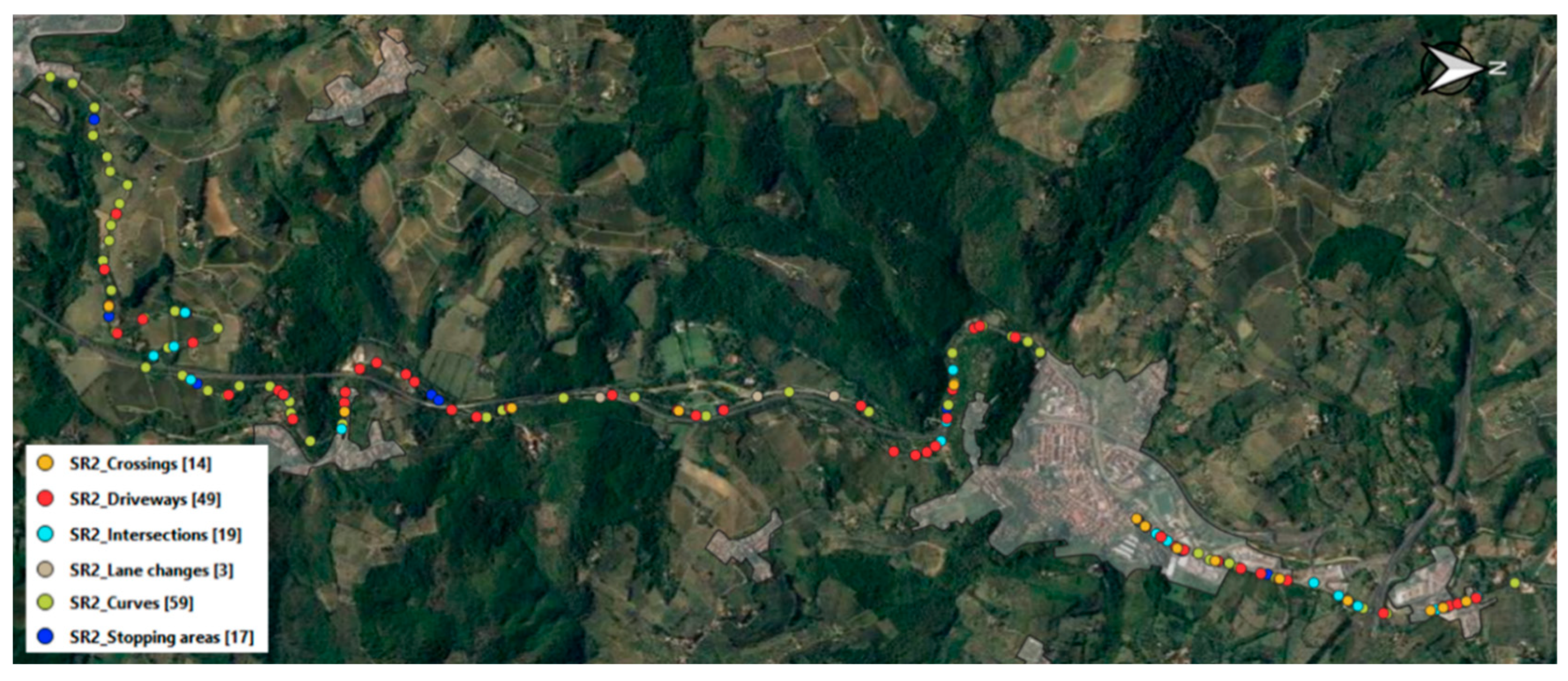
Figure 3.
Example of EXSE identification on the road SR2 stretch.
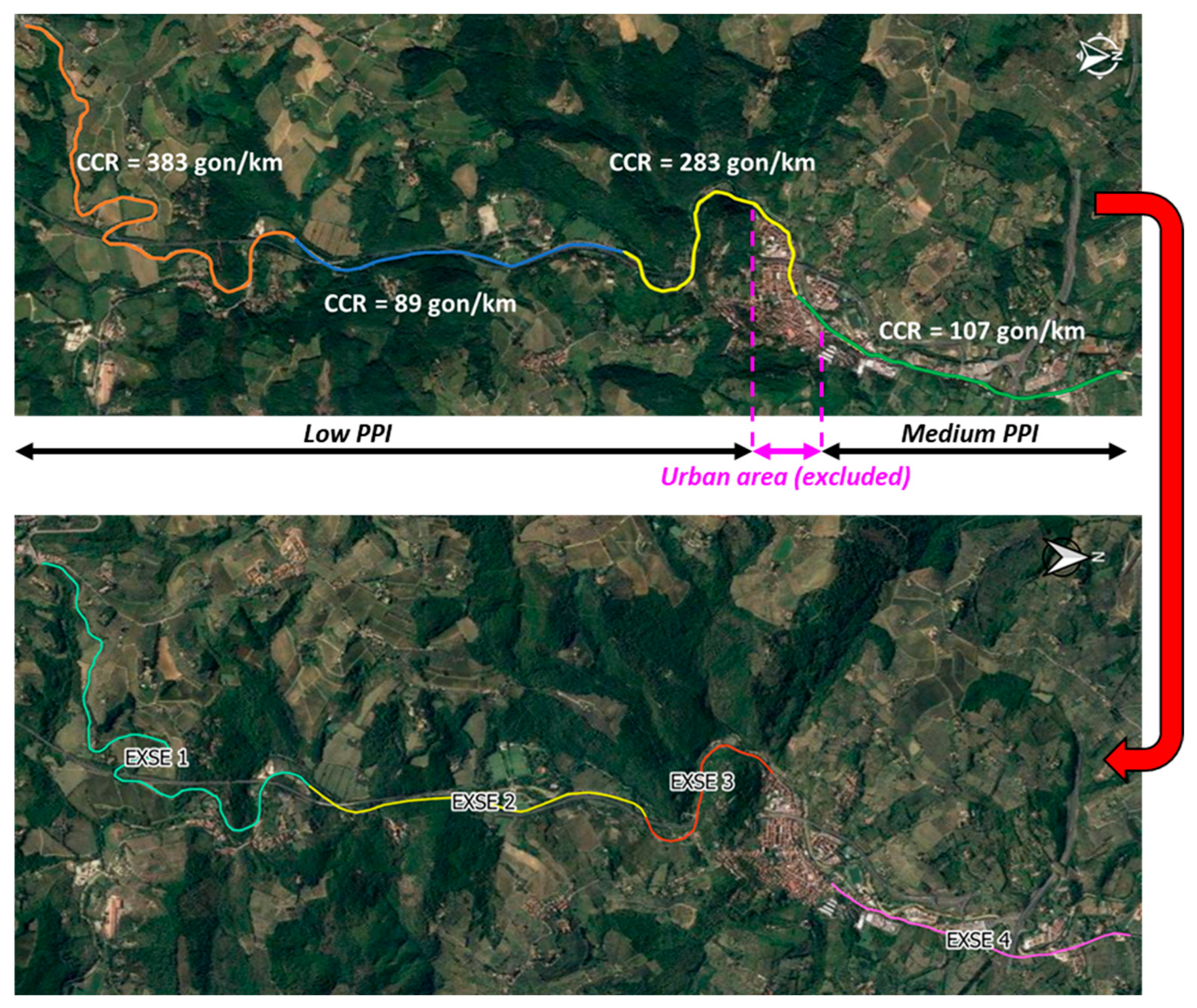
Figure 4.
Scheme of the CHT and HFES definition process.

Figure 5.
Merging of overlapping CHTs and identification of HFESs.

Figure 6.
Example of NAS composition: light blue and red lines identify HFESs in the ascending direction and descending direction, respectively (considering the Km posts). The green line is the road track.
Figure 6.
Example of NAS composition: light blue and red lines identify HFESs in the ascending direction and descending direction, respectively (considering the Km posts). The green line is the road track.

Figure 7.
Example and format of NAS final Risk Code (RC).

Figure 8.
Satellite view of the different roads.
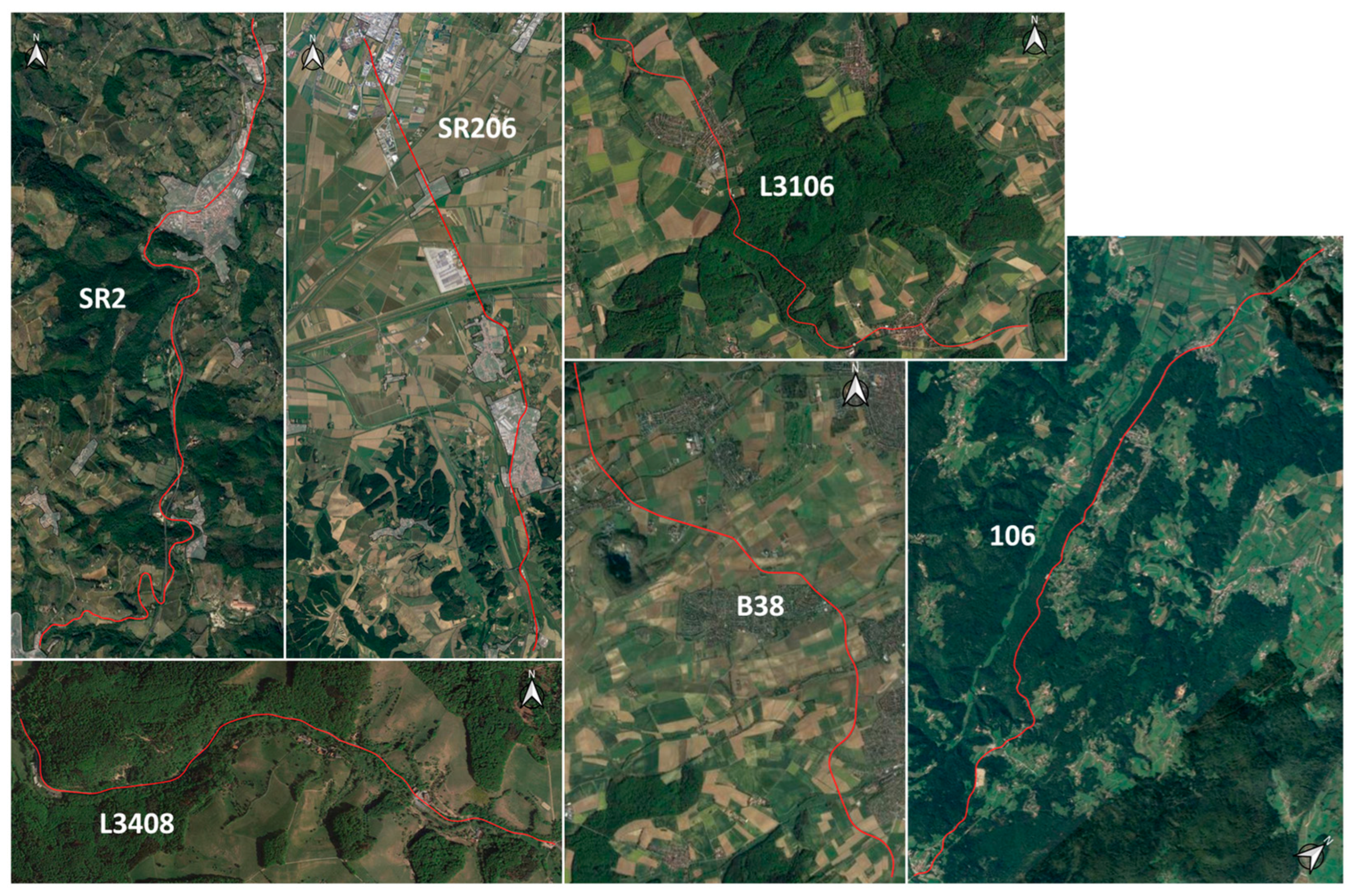
Figure 9.
Distribution and linear correlation between values assigned to the RC and accident rate values.
Figure 9.
Distribution and linear correlation between values assigned to the RC and accident rate values.

Figure 10.
Distribution and linear correlation between values assigned to the RC and accident rate values averaged within each RC.
Figure 10.
Distribution and linear correlation between values assigned to the RC and accident rate values averaged within each RC.

Figure 11.
Graphical representation of the risk level obtained for each NAS for each different NAS segmentation, road SR2.
Figure 11.
Graphical representation of the risk level obtained for each NAS for each different NAS segmentation, road SR2.

Figure 12.
Graphical representation of the risk level obtained for each NAS for each different NAS segmentation, road B38.
Figure 12.
Graphical representation of the risk level obtained for each NAS for each different NAS segmentation, road B38.


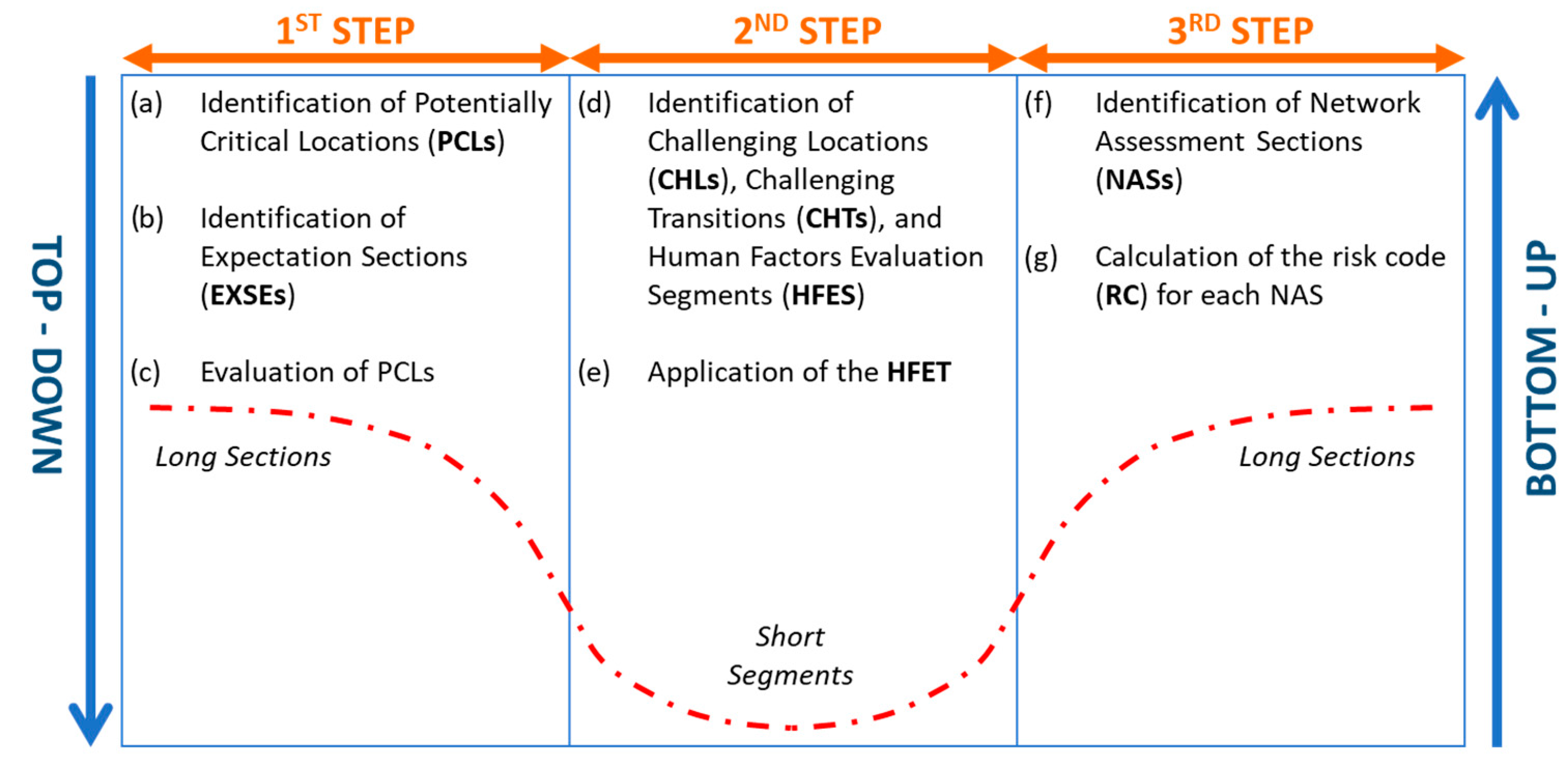
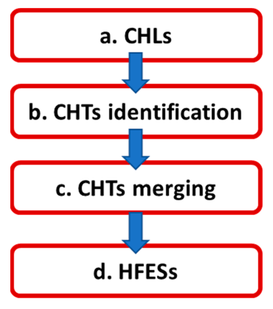
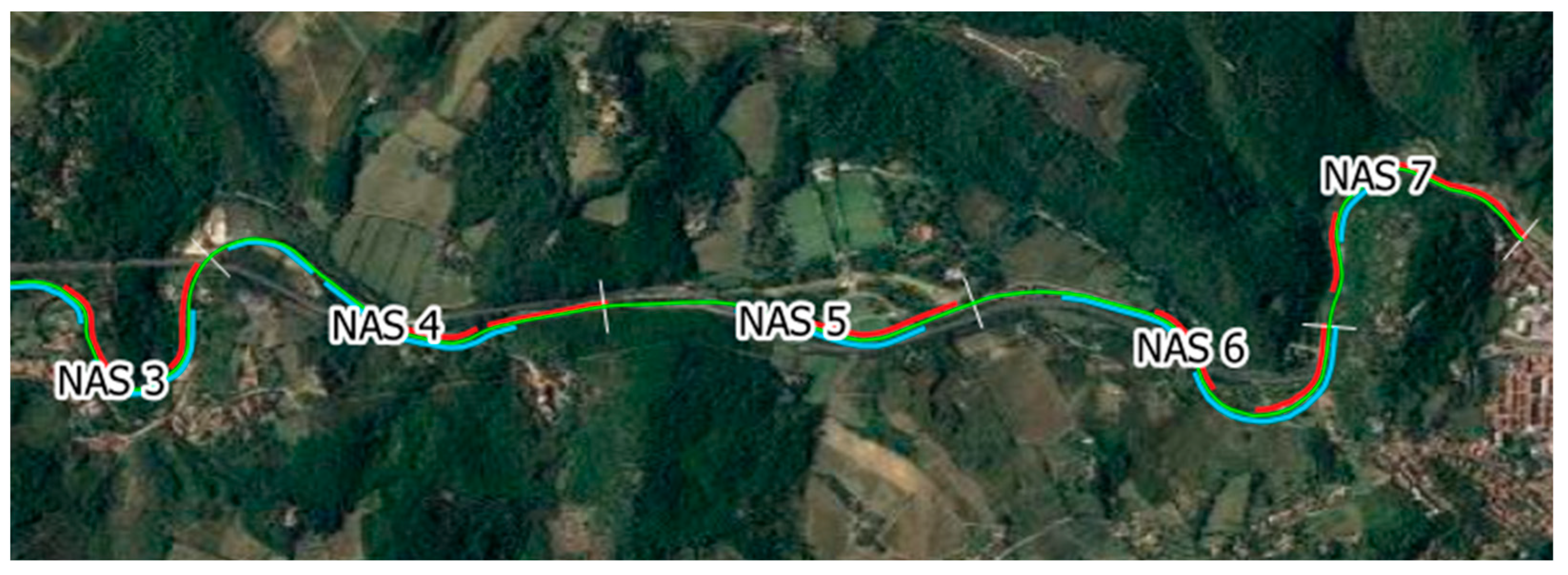
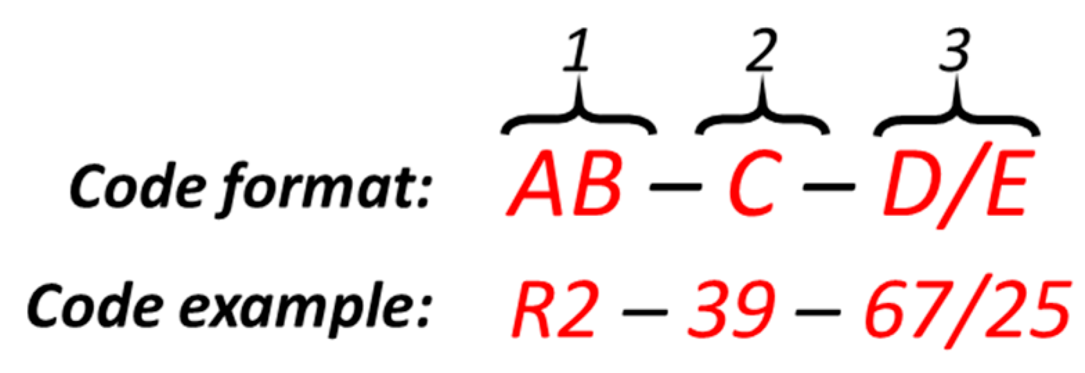
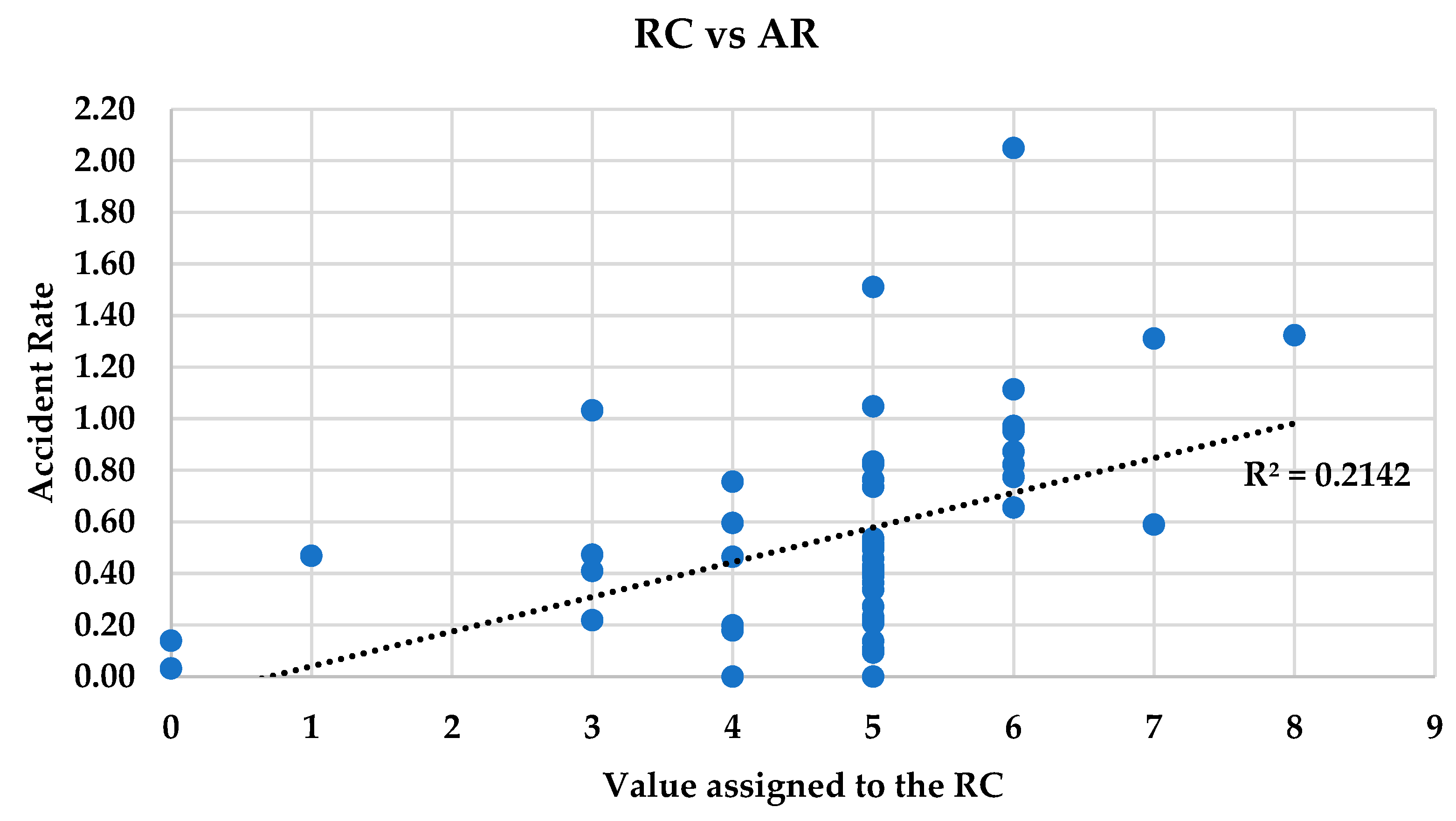
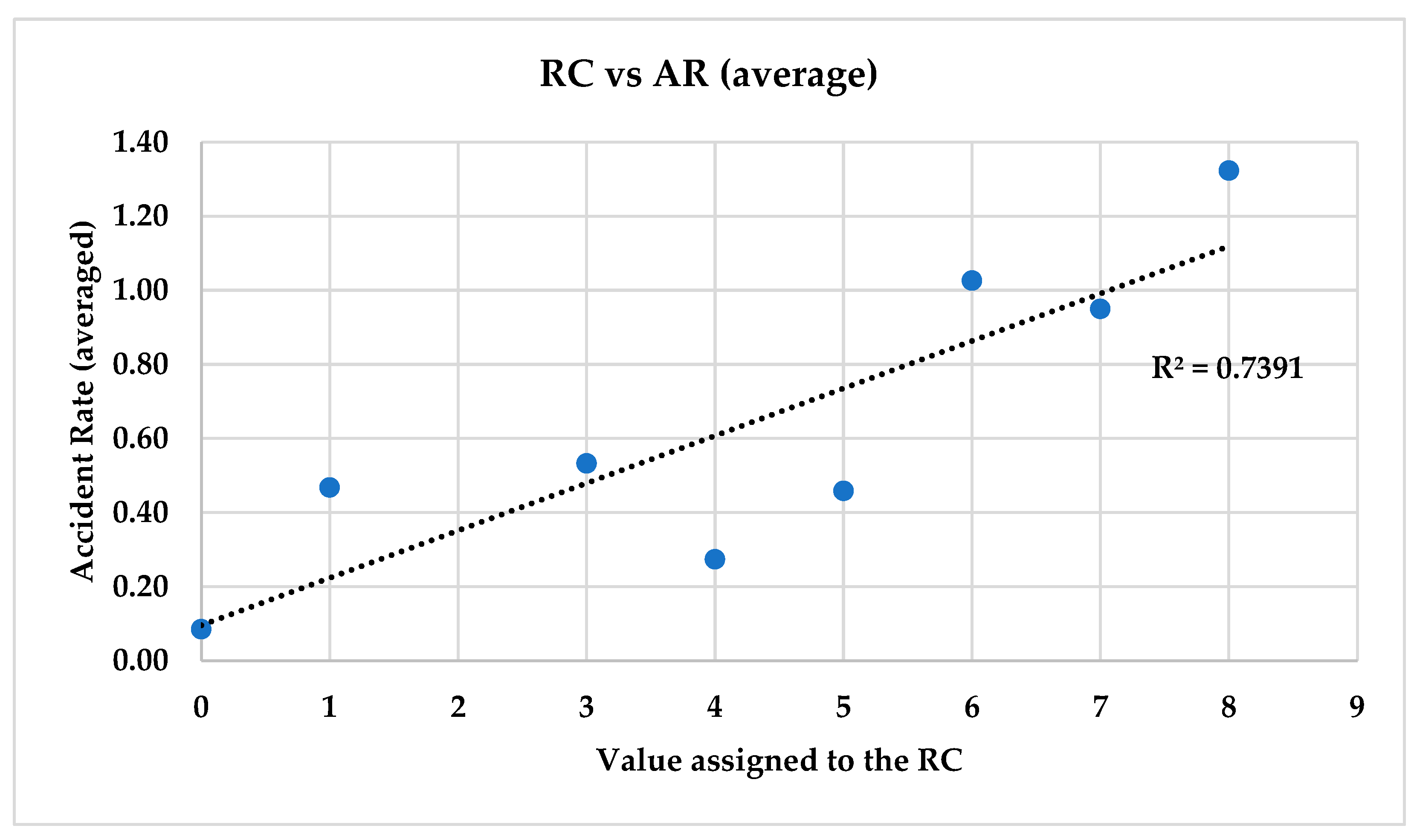
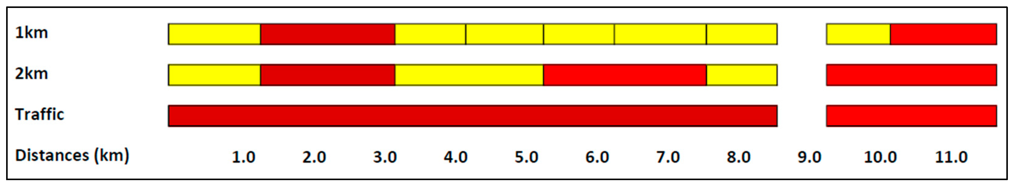
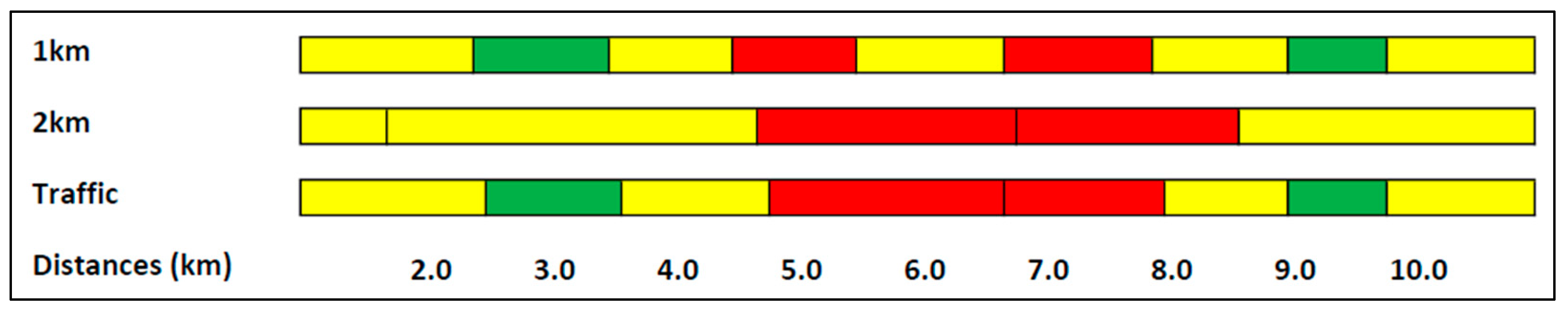
Table 1.
Level of expected speed and alertness based on winding and PPI levels.
| Road Category | Winding | PPI | VE | Alertness |
|---|---|---|---|---|
| Rural highway | H | M | M (50–80 km/h) | H |
| Rural highway | H | L | M (50–80 km/h) | M |
| Rural highway | M | M | M (50–80 km/h) | M |
| Rural highway | M | L | H (80–100 km/h) | L |
| Rural highway | L | M | M (50–80 km/h) | M |
| Rural highway | L | L | H (80–100 km/h) | L |
Table 2.
Classification of PCLs based on the level of winding and PPI.
| PCLs Type | PCLs | Winding/PPI Level (H = High, M = Medium, L = Low) | |||||
|---|---|---|---|---|---|---|---|
| L/L | L/M | M/L | M/M | H/L | H/M | ||
| Curve | Curve0 | L | L | L | L | L | L |
| Curve10 | H | H | L | L | L | L | |
| Curve20 | H | H | M | M | M | L | |
| At-grade intersection | Roundabout | M | L | M | L | M | L |
| Signalized | H | H | H | H | H | H | |
| with priority | L | L | L | L | L | L | |
| without priority | H | H | H | H | H | H | |
| Crossing | Pedestrian Crossing | H | M | H | M | H | M |
| Cyclist Crossing | H | M | H | M | H | M | |
| Driveway | Minor residential | L | L | L | L | L | L |
| Major residential | M | L | H | M | H | M | |
| Minor commercial | L | L | L | L | L | L | |
| Major Commercial | M | M | H | M | H | H | |
| Stopping area | Parking lots | H | H | H | H | H | H |
| Lay-by | L | L | L | L | M | M | |
| Bus stop | L | L | L | L | L | L | |
| Railway level crossing | With mobile bar | M | M | H | H | H | H |
| Without mobile bar | H | H | H | H | H | H | |
| Lane change | Added/removed lane | M | H | H | H | H | H |
| Diverging lane | H | H | H | H | H | H | |
Table 3.
Decision sight distance to account for VIS for each VE level: upper thresholds.
| VE Level | VE [km/h] | Max (VE) [km/h] | Min (VE) [km/h] | D2 (6 s) [m] | D2 (5 s) [m] | D2 (4 s) [m] | D1 [m] |
|---|---|---|---|---|---|---|---|
| H | 80–100 | 100 | 80 | 170 | 140 | 112 | 90 |
| M | 50–80 | 80 | 50 | 135 | 112 | 90 | 56 |
Table 4.
Aspects to consider while assessing the PEX level.
| DENSITY AND SHAPE OF THE FIELD OF VIEW |
| The monotony of road section and surroundings |
| Long/far visible approaching sections before CHL |
| ELEMENTS IN THE LATERAL ROADSIDE ENVIRONMENT SUPPORT OPTIMAL LANE-KEEPING |
| Structures above the road |
| Presence of eye-catching objects |
| Illusion-free optical guidance |
| Carriageway width changes are well-delineated |
| Roadside objects appear to be vertical |
| Curve’s framing |
| DEPTH OF FIELD VIEW |
| Dominant eye-catching objects support the detection of the challenging location |
| Presence of optical illusion |
| The course of the road is visible |
Table 5.
Combinations of VIS, GEX, and PEX levels for the identification of CHLs (X).
| Combination | 1 | 2 | 3 | 4 | 5 | 6 | 7 | 8 | 9 | 10 | 11 | 12 | 13 | 14 | 15 | 16 | 17 | 18 |
|---|---|---|---|---|---|---|---|---|---|---|---|---|---|---|---|---|---|---|
| VIS | L | M | H | L | M | H | L | M | H | L | M | H | L | M | H | L | M | H |
| GEX | H | H | H | M | M | M | L | L | L | H | H | H | M | M | M | L | L | L |
| PEX | H | H | H | H | H | H | H | H | H | L | L | L | L | L | L | L | L | L |
| Results | X | X | X | X | X | X | - | X | X | - | X | X | - | - | X | - | - | - |
Table 6.
DCHT for each VE level.
| VE Level | VE [km/h] | Max (VE)-10 [km/h] | Distance (12 s) [m] | Distance (10 s) [m] |
|---|---|---|---|---|
| H | 80–100 | 90 | 300 | 250 |
| M | 50–80 | 70 | 233 | 194 |
Table 7.
Ranking criteria within the same risk level group.
| Priority | A | B | C | D | E |
|---|---|---|---|---|---|
| Higher | R | High value | Low value | Low value | High dispersion |
| Lower | G | Low value | High value | High value | Low dispersion |
Table 8.
Summary of the results from the application of the proposed procedure and accident rate calculation, with all NASs analyzed.
Table 8.
Summary of the results from the application of the proposed procedure and accident rate calculation, with all NASs analyzed.
| Road | Name | Length [km] | AADT [veh. /day] | RC | RC Risk Level | RC Rank | AR * | AR Risk Level | AR Rank |
|---|---|---|---|---|---|---|---|---|---|
| SR2 | NAS 2 | 1.950 | 4247 | R4-34-51/25 | Very High | 1 | 1.32 | High | 3 |
| B38 | NAS 6 | 1.200 | 10,456 | R3-38-74/28 | High | 2 | 1.31 | High | 4 |
| SR2 | NAS 10 | 1.500 | 12,395 | R3-40-74/29 | High | 3 | 0.59 | Medium | 20 |
| 106 | NAS 14 | 1.200 | 8369 | R2-39-73/29 | High | 4 | 0.87 | High | 10 |
| L3106 | NAS 3 | 1.250 | 1783 | R2-41-68/26 | High | 5 | 2.05 | High | 1 |
| 106 | NAS 7 | 1.000 | 8369 | R2-41-80/26 | High | 6 | 1.11 | High | 5 |
| L3106 | NAS 6 | 1.140 | 2922 | R2-42-58/22 | High | 7 | 0.82 | Medium | 12 |
| 106 | NAS 10 | 1.100 | 8369 | R2-42-72/28 | High | 8 | 0.95 | High | 9 |
| 106 | NAS 6 | 1.100 | 8369 | R2-43-54/20 | High | 9 | 0.77 | High | 14 |
| 106 | NAS 2 | 1.300 | 8369 | R2-44-60/23 | High | 10 | 0.65 | Medium | 18 |
| B38 | NAS 4 | 1.000 | 14,098 | R2-45-73/27 | High | 11 | 0.97 | High | 8 |
| SR206 | NAS 5 | 1.300 | 11,799 | R1-40-54/23 | Medium | 12 | 0.43 | Medium | 29 |
| SR2 | NAS 6 | 1.250 | 4247 | R1-40-64/28 | Medium | 13 | 0.21 | Medium | 43 |
| B38 | NAS 5 | 1.200 | 10,179 | R1-40-68/26 | Medium | 14 | 0.82 | High | 13 |
| L3106 | NAS 1 | 0.800 | 3024 | R1-40-70/26 | Medium | 15 | 1.51 | High | 2 |
| L3408 | NAS 2 | 1.410 | 3311 | R1-41-67/25 | Medium | 16 | 0.39 | Medium | 34 |
| 106 | NAS 13 | 1.200 | 8369 | R1-41-73/27 | Medium | 17 | 0.76 | High | 15 |
| L3408 | NAS 1 | 1.500 | 3311 | R1-41-77/25 | Medium | 18 | 0.74 | Medium | 17 |
| SR206 | NAS 1 | 1.300 | 11,799 | R1-41-79/26 | Medium | 19 | 0.21 | Low | 41 |
| SR206 | NAS 10 | 1.050 | 11,799 | R1-41-80/27 | Medium | 20 | 0.40 | Medium | 33 |
| SR206 | NAS 7 | 1.100 | 11,799 | R1-42-50/20 | Medium | 21 | 0.21 | Low | 42 |
| SR2 | NAS 3 | 0.950 | 4247 | R1-42-63/27 | Medium | 22 | 0.27 | Medium | 38 |
| 106 | NAS 9 | 1.000 | 8369 | R1-42-68/29 | Medium | 23 | 1.05 | High | 6 |
| L3106 | NAS 4 | 1.250 | 1783 | R1-42-73/25 | Medium | 24 | 0.41 | Medium | 31 |
| 106 | NAS 12 | 1.100 | 8369 | R1-43-71/27 | Medium | 25 | 0.83 | High | 11 |
| 106 | NAS 15 | 0.900 | 8369 | R1-43-74/28 | Medium | 26 | 0.36 | Medium | 36 |
| SR2 | NAS 9 | 0.750 | 12,395 | R1-43-74/26 | Medium | 27 | 0.41 | Medium | 30 |
| SR206 | NAS 2 | 1.350 | 11,799 | R1-44-55/20 | Medium | 28 | 0.14 | Low | 47 |
| SR2 | NAS 4 | 1.150 | 4247 | R1-44-70/26 | Medium | 29 | 0.34 | Medium | 37 |
| B38 | NAS 9 | 1.190 | 12,021 | R1-44-73/25 | Medium | 30 | 0.51 | Medium | 23 |
| SR206 | NAS 12 | 1.100 | 15,335 | R1-44-84/25 | Medium | 31 | 0.39 | Medium | 35 |
| SR2 | NAS 5 | 1.000 | 4247 | R1-45-76/26 | Medium | 32 | 0.52 | Medium | 22 |
| SR206 | NAS 9 | 1.000 | 11,799 | R1-46-73/27 | Medium | 33 | 0.09 | Low | 49 |
| SR2 | NAS 7 | 0.900 | 4247 | R1-46-74/26 | Medium | 34 | 0.00 | Low | 52 |
| SR206 | NAS 4 | 1.000 | 11,799 | R1-46-93/18 | Medium | 35 | 0.23 | Low | 39 |
| 106 | NAS 1 | 1.000 | 8369 | R1-47-82/22 | Medium | 36 | 0.46 | Medium | 28 |
| 106 | NAS 8 | 1.100 | 8369 | R1-47-87/22 | Medium | 37 | 0.54 | Medium | 21 |
| SR2 | NAS 1 | 1.200 | 4247 | R1-47-92/18 | Medium | 38 | 0.11 | Low | 48 |
| B38 | NAS 3 | 1.000 | 11,078 | R1-64-93/14 | Medium | 39 | 0.49 | Medium | 24 |
| L3106 | NAS 2 | 0.800 | 3024 | Y4-42-71/25 | Medium | 40 | 0.00 | Low | 53 |
| SR206 | NAS 6 | 1.100 | 11,799 | Y4-43-76/27 | Medium | 41 | 0.00 | Low | 54 |
| 106 | NAS 3 | 1.300 | 8369 | Y4-45-74/26 | Medium | 42 | 0.76 | High | 16 |
| B38 | NAS 7 | 1.100 | 10,732 | Y4-46-81/25 | Medium | 43 | 0.46 | Medium | 27 |
| B38 | NAS 1 | 1.300 | 7068 | Y4-47-81/23 | Medium | 44 | 0.20 | Medium | 44 |
| L3106 | NAS 5 | 1.050 | 2922 | Y4-47-84/22 | Medium | 45 | 0.60 | Medium | 19 |
| SR206 | NAS 13 | 1.200 | 15,335 | Y4-47-94/16 | Medium | 46 | 0.18 | Low | 45 |
| SR206 | NAS 3 | 0.950 | 11,799 | Y4-48-90/20 | Medium | 47 | 0.00 | Low | 51 |
| 106 | NAS 11 | 0.800 | 8369 | Y3-52-73/22 | Low | 48 | 0.41 | Medium | 32 |
| 106 | NAS 4 | 1.200 | 8369 | Y3-53-93/17 | Low | 49 | 0.22 | Low | 40 |
| B38 | NAS 8 | 0.700 | 11,377 | Y3-57-79/21 | Low | 50 | 1.03 | High | 7 |
| B38 | NAS 2 | 1.200 | 8058 | Y3-58-75/20 | Low | 51 | 0.47 | Medium | 25 |
| 106 | NAS 5 | 0.700 | 8369 | Y1-61-94/14 | Low | 52 | 0.47 | Medium | 26 |
| SR206 | NAS 11 | 1.150 | 15,335 | G4-100-100/00 | Low | 53 | 0.03 | Low | 50 |
| SR206 | NAS 8 | 1.000 | 11,799 | G4-100-100/00 | Low | 54 | 0.14 | Low | 46 |
* [acc./(km∙Mvehicles∙year)].
Table 9.
Contingency table for all NASs. T green cells highlight those sections that do not require any interventions. The red cell highlights those sections that require interventions.
Table 9.
Contingency table for all NASs. T green cells highlight those sections that do not require any interventions. The red cell highlights those sections that require interventions.
| Contingency Table | Accident Rate | ||||
|---|---|---|---|---|---|
| Low | Medium | High | Tot. | ||
| Proposed procedure | Low | 3 | 3 | 1 | 7 |
| Medium | 11 | 19 | 6 | 36 | |
| High | 0 | 3 | 8 | 11 | |
| Tot. | 14 | 25 | 15 | 54 | |
Table 10.
Relationship between the RC index and the value considered for the regression analysis.
| Code | Associated Value |
|---|---|
| R4 | 8 |
| R3 | 7 |
| R2 | 6 |
| R1 | 5 |
| Y4 | 4 |
| Y3 | 3 |
| Y2 | 2 |
| Y1 | 1 |
| Z4 | 0 |
Table 11.
Comparison of the results of the procedure carried out by different teams on the same road (SR2).
Table 11.
Comparison of the results of the procedure carried out by different teams on the same road (SR2).
| Name | AADT [Veh. /Day] | Team 1 | Team 2 | ||||||
|---|---|---|---|---|---|---|---|---|---|
| Length [km] | RC | RC Risk Level | RC Rank | Length [km] | RC | RC Risk Level | RC Rank | ||
| NAS 1 | 4247 | 1.200 | R1-47-92/18 | Medium | 9 | 1.100 | R1-51-72/21 | Medium | 8 |
| NAS 2 | 4247 | 1.950 | R4-34-51/25 | Very High | 1 | 1.750 | R4-34-56/26 | Very High | 1 |
| NAS 3 | 4247 | 0.950 | R1-42-63/27 | Medium | 4 | 0.900 | R1-45-69/26 | Medium | 6 |
| NAS 4 | 4247 | 1.150 | R1-44-70/26 | Medium | 6 | 0.950 | R1-45-61/24 | Medium | 4 |
| NAS 5 | 4247 | 1.000 | R1-45-76/26 | Medium | 7 | 1.100 | R1-47-67/23 | Medium | 7 |
| NAS 6 | 4247 | 1.250 | R1-40-64/28 | Medium | 3 | 1.330 | R1-42-73/26 | Medium | 3 |
| NAS 7 | 4247 | 0.900 | R1-46-74/26 | Medium | 8 | 1.230 | R1-45-62/22 | Medium | 5 |
| NAS 9 | 12,395 | 0.750 | R1-43-74/26 | Medium | 5 | 0.750 | Y4-52-72/23 | Medium | 9 |
| NAS 10 | 12,395 | 1.500 | R3-40-74/29 | High | 2 | 1.100 | R3-36-58/25 | High | 2 |
Table 12.
Comparison of the results of the previous version of the procedure from Paliotto et al. [49] and the actual procedure.
Table 12.
Comparison of the results of the previous version of the procedure from Paliotto et al. [49] and the actual procedure.
| Previous Version | Actual Version | ||||||
|---|---|---|---|---|---|---|---|
| Road | Name | Length [km] | RC | Risk Level | Length [km] | RC | Risk Level |
| SR2 | NAS 2 | 1.950 | R4-34-54/24 | Very High | 1.950 | R4-34-51/25 | Very High |
| B38 | NAS 6 | 1.200 | R3-38-71/28 | High | 1.200 | R3-38-74/28 | High |
| SR2 | NAS 10 | 1.250 | R3-41-75/28 | High | 1.500 | R3-40-74/29 | High |
| 106 | NAS 14 | 1.200 | R2-35-72/30 | High | 1.200 | R2-39-73/29 | High |
| 106 | NAS 7 | 1.000 | R2-41-80/26 | High | 1.000 | R2-41-80/26 | High |
| 106 | NAS 10 | 1.100 | R2-42-72/28 | High | 1.100 | R2-42-72/28 | High |
| 106 | NAS 6 | 1.100 | R2-43-54/20 | High | 1.100 | R2-43-54/20 | High |
| 106 | NAS 2 | 1.300 | R2-44-60/23 | High | 1.300 | R2-44-60/23 | High |
| B38 | NAS 4 | 1.000 | R1-45-74/26 | Medium | 1.000 | R2-45-73/27 | High |
| SR2 | NAS 6 | 1.250 | R1-46-72/22 | Medium | 1.250 | R1-40-64/28 | Medium |
| B38 | NAS 5 | 1.200 | R1-40-68/25 | Medium | 1.200 | R1-40-68/26 | Medium |
Disclaimer/Publisher’s Note: The statements, opinions and data contained in all publications are solely those of the individual author(s) and contributor(s) and not of MDPI and/or the editor(s). MDPI and/or the editor(s) disclaim responsibility for any injury to people or property resulting from any ideas, methods, instructions or products referred to in the content. |
© 2024 by the authors. Licensee MDPI, Basel, Switzerland. This article is an open access article distributed under the terms and conditions of the Creative Commons Attribution (CC BY) license (https://creativecommons.org/licenses/by/4.0/).
Share and Cite
MDPI and ACS Style
Paliotto, A.; Meocci, M. Development of a Network-Level Road Safety Assessment Procedure Based on Human Factors Principles. Infrastructures 2024, 9, 35. https://doi.org/10.3390/infrastructures9020035
AMA Style
Paliotto A, Meocci M. Development of a Network-Level Road Safety Assessment Procedure Based on Human Factors Principles. Infrastructures. 2024; 9(2):35. https://doi.org/10.3390/infrastructures9020035
Chicago/Turabian StylePaliotto, Andrea, and Monica Meocci. 2024. "Development of a Network-Level Road Safety Assessment Procedure Based on Human Factors Principles" Infrastructures 9, no. 2: 35. https://doi.org/10.3390/infrastructures9020035