
patchIT: A Multipurpose Patch Creation Tool for Image Processing Applications


Department of Surveying and Geoinformatics Engineering, University of West Attica, 12243 Athens, Greece
*
Author to whom correspondence should be addressed.
Multimodal Technol. Interact. 2022, 6(12), 111; https://doi.org/10.3390/mti6120111
Submission received: 10 November 2022
/
Revised: 11 December 2022
/
Accepted: 12 December 2022
/
Published: 14 December 2022
(This article belongs to the Special Issue Feature Papers in Multimodal Technologies and Interaction—Edition 2023)
Abstract
:Patch-based approaches in image processing are often preferable to working with the entire image. They provide an alternative representation of the image as a set of partial local sub-images (patches) which is a vital preprocessing step in many image processing applications. In this paper, a new software tool called patchIT is presented, providing an integrated framework suitable for the systematic and automatized extraction of patches from images based on user-defined geometrical and spatial criteria. Patches can be extracted in both a sliding and random manner and can be exported either as images, MATLAB .mat files, or raw text files. The proposed tool offers further functionality, including masking operations that act as spatial filters, identifying candidate patch areas, as well as geometric transformations by applying patch value indexing. It also efficiently handles issues that arise in large-scale patch processing scenarios in terms of memory and time requirements. In addition, a use case in cartographic research is presented that utilizes patchIT for map evaluation purposes based on a visual heterogeneity indicator. The tool supports all common image file formats and efficiently processes bitonal, grayscale, color, and multispectral images. PatchIT is freely available to the scientific community under the third version of GNU General Public License (GPL v3) on the GitHub platform.
1. Introduction
Patch-based image processing techniques have attracted increasing attention during the last year, as they have been applied in various scientific fields in physical, medical, and environmental sciences. Patch-based algorithms first split an image into several smaller images (generally rectangular), called patches, and in a second step, they process these patches individually or collectively. Their utilization in image processing has been shown to produce significant results in multiple domains, including image denoising, remote sensing, medical image analysis, multiscale image restoration, and object detection, among many others [1,2,3,4,5,6,7,8,9,10]. Recently, the evolution of convolutional neural networks (CNN) has further extended the applicability of patch-based methods. For example, deep features can be extracted from irregular image objects through CNN by utilizing a patch-based approach to represent image objects and learn patch-based deep features, whereas a deep feature aggregation method can be utilized to aggregate patch-based deep features into object-based deep features [4]. In addition, a patch-based recurrent neural network (PB-RNN) system tailored to classifying multitemporal remote sensing data can be used to process remote sensing images [5]. In another work, a novel patch-wise semantic segmentation method with a new training strategy based on fully convolutional networks was presented to segment common land resources [6]. Another research study proposed and applied a patch-based light convolutional neural network (LCNN), which was well-fitted for medium-resolution land-cover classification and mapping [7]. In this study, aside from pixel-based sampling, patch-based spatial sampling was also performed to create land-cover classifications and maps. The results of this study confirmed the superiority of patch-based classification results compared to pixel-based classification in terms of accuracy.
In several recent publications, patch-based methods were successfully applied in medical image processing applications. For instance, a generic approach to address fully automatic segmentation of brain tumors using multi-atlas patch-based voting techniques was proposed by Cordier et al. [8]. Khawaja et al. [9] recently proposed a state-of-the-art probabilistic patch-based (PPB) denoiser for vessel segmentation, which is based on an unsupervised retinal vessel segmentation strategy and the Frangi filter. In addition, patch-based methods have been extensively implemented for magnetic resonance imaging (MRI) reconstruction [10], segmentation [11], denoising [12], and brain tumor detection [13]. Furthermore, tools and libraries based on Python have been developed in the specific case of MRI, which can be used for patch-based sampling in deep learning [14].
Remote sensing is another important field in which state-of-the-art technological applications based on 3D laser scanners and digital cameras have led to significant advances in computer vision. Barnes and Zhang recently reviewed patch-based synthesis methods in this field [15]. Multiview stereo (MVS) dense reconstruction utilizing patch-based methods has been proposed in image-based 3D acquisition [16,17]. In addition, patch-based density forecasting networks were developed in order to forecast crowd density maps from public datasets of surveillance videos [18], and drone-acquired forest images were analyzed by deep learning techniques implementing a patch-based framework [19]. In another example of the application of patch-based methods, laser speckle contrast imaging was studied using deep neural networks to detect known and unknown fingerprint presentation attacks [20].
Considering the wide range of domains and applications in which patch-based methods and techniques are potentially involved, the development of a multipurpose software tool to efficiently create patches based on a variety of user-defined criteria is an important and beneficial task. In this work, a new MATLAB tool called patchIT is presented. It enables the systematic extraction of patches from images based on user-defined geometrical and spatial criteria. The proposed tool provides a unified framework that facilitates patch-oriented operations that can be applied to all common image file formats, supporting bitonal, grayscale, color, and multispectral images. PatchIT is utilized in an easy-to-adapt, functional form that can be used to:
- Extract patches both in sliding and random mode controlled by user-defined parameters regarding the patch size, stride, and distribution along the source image;
- Export the patches either directly to image files of various types, in a compact representation as MATLAB .mat files, or as raw text files that can be easily loaded and edited for further processing and maintenance;
- Involve masking techniques that act as spatial filters, identifying candidate patch areas;
- Apply patch-level geometric transformations;
- Reorder the patch intensities by user-defined patch value indexing, offering deeper low-level information insights.
Because the number of created patches is a combination of various parameters that affect the workload both in terms of memory and time requirements, patchIT provides alternative processing modes that efficiently handle the applicability issues that arise in large-scale patch processing scenarios.
In order to demonstrate the applicability of the tool in a realistic scenario and evaluate its functionality in the case of a large dataset, cartographic backgrounds characterized by different scale levels are utilized for the investigation of map visual heterogeneity. In cartographic research, the quantification of map visual complexity constitutes a challenging process, and over the years, map complexity has been examined according to various concepts (e.g., [21,22]), including visual perception (e.g., [23,24,25,26]). In this work, visual heterogeneity is used as an indicator of map visual complexity, demonstrating that map visual heterogeneity is affected by map scale level. The Shannon entropy of the generated patches is implemented as an indicator of visual heterogeneity as proposed by Merlemis et al. [27].
The rest of this paper is organized as follows: Section 2 introduces the basic operations that refer to the creation and saving of the patches. Section 3 describes further functionality provided by the tool regarding mask filtering, geometric transformations, patch indexing, and operational modes. Experimental results of a use case in cartographic research are provided in Section 4, and a discussion follows in Section 5 that highlights the applicability of the proposed tool, in additional patch-oriented applications. Finally, conclusions are drawn in Section 6.
2. Basic Operations
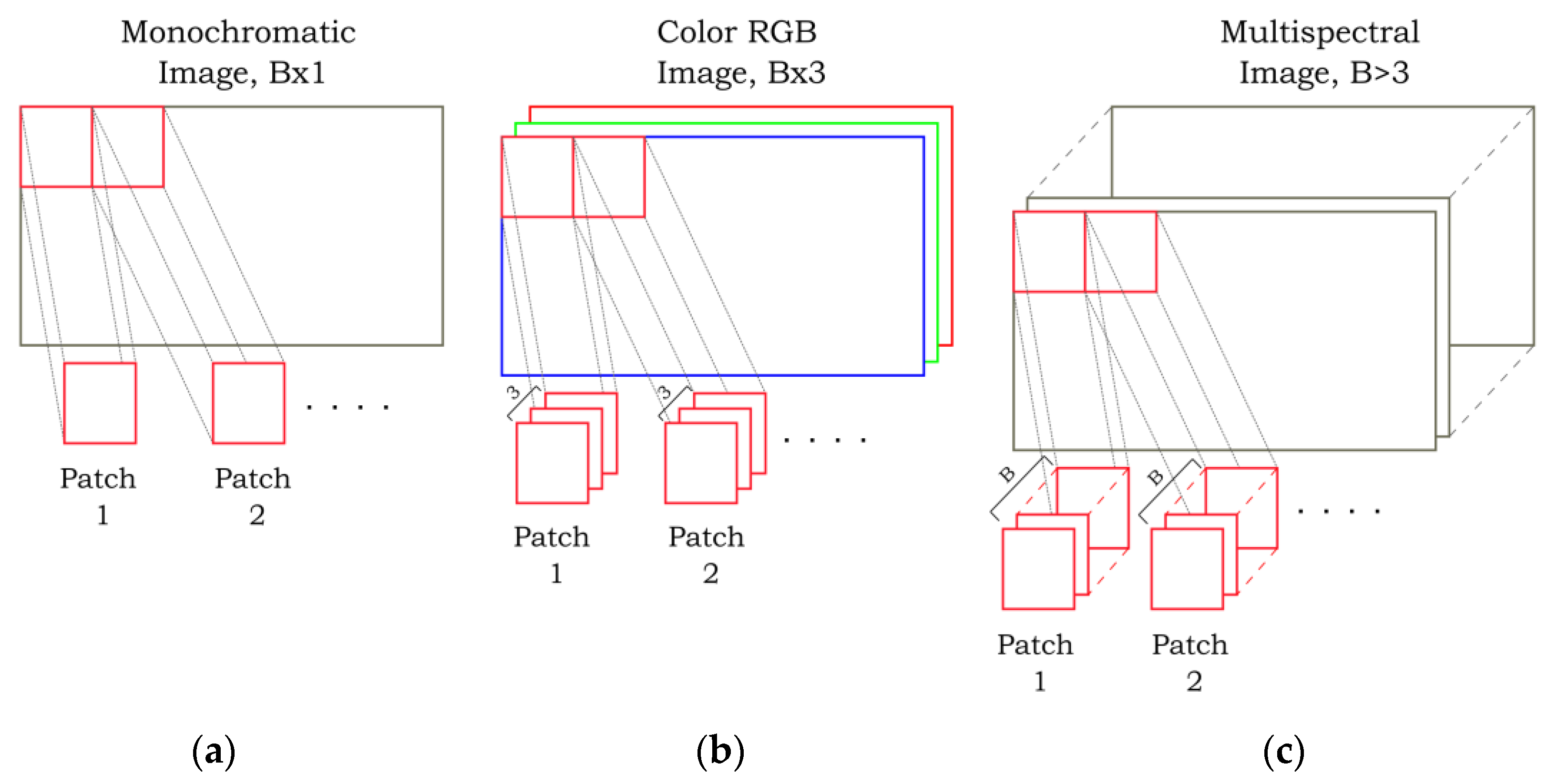
Patch extraction provides a representation of an image as a set of partial local sub-images (patches) and is a vital preprocessing step in many image processing application. Specifically, an image () is divided into patches (), where and denote the dimensions (width × height) of the image and the patch, respectively, whereas denotes the number of image bands. In a monochromatic image, , and in a typical color image, , whereas in a multispectral image, is a number greater than 3. Patches are often square-shaped, that is, and are usually much smaller than the image, that is, and . It should be noted that for , patches are created in an image cube fashion. This means that a patch concatenates all the bands in a 3D manner so that for each patch pixel, the entire spectral information is provided as planes in the “third” dimension. Figure 1 illustrates the patch extraction process for various image types.
2.1. Patch Creation
The patchIT function, in its simplest syntax, requires two parameters: the input image and the patch size. For example, the command
patchit(‘sample512.jpg’,[50 30]);
defines sample512.jpg as the input image and sets the patch size equal to 50 pixels in width and 30 pixels in height. The input image can be provided either as a string that defines the image file name or as a MATLAB variable. Thus, the above command can be alternatively written as
I=imread(‘sample512.jpg’);
patchit(I,[50 30]);
An input image can be any bitonal, grayscale, color, or multispectral image that can be imported into MATLAB. Several standard file formats are supported, including the Joint Photographic Experts Group (JPEG), portable network graphics (PNG), tagged image file format (TIFF), and graphics interchange format (GIF) formats. The patch size is a two-valued vector that defines the width W and the height H (in pixels) of the patch.
The patchIT tool offers two modes for patch creation defined by the Mode parameter. In sliding mode, patches are created in a grid-like fashion; the distance between patches can be precisely defined both in the horizontal and vertical directions. This approach produces patches that may overlap, are densely allocated, or have a distance between them. In random mode, the patches are randomly distributed all over the image following user-defined criteria, such as the number of patches, their proximity, and their spatial distribution.
2.1.1. Sliding Mode
By default, patchIT extracts patches in a dense, non-overlapping mode. For example, the command
patchit(‘sample512.jpg’,[128 128],’Mode’,’sliding’);
or simply
patchit(‘sample512.jpg’,[128 128]);
divides the 512 × 512 input image, sample512.jpg, into 16 dense, non-overlapping patches with dimensions of 128 × 128, as shown in Figure 2a. In order to extract patches allocated with an arbitrary distance between them, the Stride parameter should be involved. This parameter is provided as a two-valued vector () that defines the offset between patches in the horizontal and vertical directions. For instance, the command
patchit(‘sample512.jpg’,[128 128],’Stride’,[192 192]);
extracts patches with dimensions of 128 × 128 that have a horizontal and vertical offset of pixels. This leads to patches with a 64-pixel gap between them in both directions, as shown Figure 2b. On the other hand, in the command
patchit(‘sample512.jpg’,[128 128],’Stride’,[192 96]);
the Stride value for the axis is changed to pixels, resulting in patches that are still 64 pixels apart in the direction but overlap for 32 pixels in the direction, as shown in Figure 2c. The example shown in Figure 2d corresponds to the command
patchit(‘sample512.jpg’,[128 128],’Stride’,[64 64]);
where the patches overlap for 64 pixels in both directions.
Figure 2.
Examples of controlling the offset between patches using the Stride parameter: (a) dense, non-overlapping patches without gaps; (b) patches with the same gap between them in both directions; (c) patches that overlap only in the direction; (d) patches that overlap in both directions. Image sample512.jpg has dimensions M × Ν = 512 × 512, and the patch size is W × H = 128 × 128. Patches are marked as red squares, and blue dots denote patch centers.

The overall number of created patches is
where denotes the least integer greater than or equal to . If the Stride parameter is omitted, its value is set to be equal to the patch size. Thus, the command
patchit(‘sample512.jpg’,[128 128],’Stride’,[128 128]);
is equivalent to
patchit(‘sample512.jpg’,[128 128]);
which corresponds to densely non-overlapping patches such as those shown in Figure 2a.
It should be noted that the overall number of patches increases significantly as the patch size and the stride decrease. Table 1 summarizes the number of patches created for several combinations of patch and stride size in a medium-sized image of 512 × 512 pixels and an 4K image with dimensions of 3840 × 2160 pixels. The last row refers to the limiting scenario (although very common in many applications) of patches that slide one pixel in both directions. It is obvious that even in a medium-sized 512 × 512 image, the number of patches reach 250,000 for an 8 × 8 patch size. This number increases to 8.2 million patches in the case of a 4K image.
Accordingly, the memory requirements grow even faster as the stride decreases and the patch size remains large. Table 2 demonstrates similar results for various patch and stride size combinations. In the case of one-pixel stride, the memory requirements for a typical patch of size 128 × 128 in a 4K image are approximately 117 GB for a monochromatic image (assuming 1 byte per pixel). These results highlight the importance of selecting a proper output methodology in order to keep the patch creation process feasible both in terms of time and memory requirements.
2.1.2. Random Mode
In this mode, the patches are randomly positioned all over the image. This mode is enabled by setting the parameter Mode to random. The number of required patches is provided by the parameter Count. For example, the command
patchit(‘sample512.jpg’,[64 64],’Μode’,’random’,’Count’,15);
creates 15 patches with dimensions of 64 × 64 pixels randomly positioned all around the source image, as shown in Figure 3a. The default Count value is 10 patches. As depicted in the figure, some of the patches may partially overlap. The maximum percentage of allowed overlap can be defined by setting the parameter RandomMaxOverlap to a value between 0 (no overlap allowed) and 1 (any patch position is allowed). The value is expressed as a percentage of the patch area. For example, if the patch size is 64 × 64 pixels and the RandomMaxOverlap value is 0.25, then a maximum of (64 × 64)·25% = 1024 pixels overlap is allowed among patches.
A combination of large patch size, small image dimensions, large patch count, and low RandomMaxOverlap value may render the patch extraction process disproportionately difficult or even infeasible. The parameter RandomAttempts defines a maximum number of attempts to be performed in order to achieve a feasible solution. For example, the command
patchit(‘sample512.jpg’,[128 128],’Mode’,’random’,’Count’,5,…
‘RandomMaxOverlap’,0.1,’RandomAttempts’,50);
attempts to extract five random patches with dimensions of 128 × 128 pixels that are allowed to overlap up to 10% of their area, as shown in Figure 3b. If the maximum number of 50 attempts is reached, an error message appears, and the process stops.
2.2. Saving Patches
This section describes the various patch-saving options provided by the patchIT tool. Patches can be saved either as image files, as a MATLAB (*.mat) file, or as a text-format file. The first option is the evident one that provides the extracted patches directly in image format, ready for further processing and analysis. The second option results in a typical MATLAB .mat file in which all patches are stored in a unified form in one multidimensional variable. Finally, the last option extracts all multiband pixel intensity information of all patches in a text format that can be easily loaded and edited for further processing and maintenance. The method used to save the extracted patches is defined by the SaveMode parameter, with three possible values, namely images, mat, or raw. Each method has its own characteristics and advantages, and an appropriate choice depends on a combination of application requirements and time/memory restrictions.
2.2.1. Image Files
Saving the patches as image files is the most common approach, whereby each patch is saved to a separate image file capable of readily being shown in any image viewer. For this purpose, the SaveMode parameter has to be set to images. For example, the command
patchit(‘sample512.jpg’,[128 128],’Stride’,[64 64],… ‘SaveMode’,’images’);
creates 49 separate image files in the current folder, each one containing a certain patch. By default, the patches are saved in auto-numbered *.PNG image files named patch1.png, patch2.png, etc. The default image file type can be modified using the parameter SaveImagesExt. For instance, the command
patchit(‘sample512.jpg’,[128 128],’Stride’,[64 64],… ‘SaveMode’,’images’,’SaveImagesExt’,’tif’);
saves the patches in TIF format. Alternatively, the parameter SaveImagesTemplate can be used that provides more flexibility, as it predefines the filename prefix, the image file format, and the numbering pattern. For example, the command
patchit(‘sample512.jpg’,[128 128],’Stride’,[64 64],… ‘SaveMode’,’images’,’SaveImagesTemplate’,’patchfile000.jpg’);
saves the patches in JPG format using the prefix patchfile followed by a three-digit pattern, such as patchfile001.jpg, patchfile002.jpg, etc.
Besides the patch image files, an additional pos.txt file that contains the coordinates of all patches is created. This text file includes N lines (one per patch), where each line consisting of four values (x1, y1, x2, y2) corresponds to the top-left and bottom-right coordinates of the respective patch. Once created, the pos.txt file can be easily imported using the load command, which creates a variable named pos in the MATLAB workspace. For example, the position of the 15th patch on the image is provided by command pos(15,:), returning a four-value vector that denotes its top-left and bottom-right coordinates.
Although saving patches directly to image files is an efficient and convenient way to visualize and explore the extracted patches, it should be noted that, according to Table 1, various combinations of image size, patch size, and stride may potentially result in a very large number of patch files. In this case, saving the patches to a .mat MATLAB file should be considered, as this option offers a more compact representation.
2.2.2. MATLAB .Mat File
This is the default option that saves the extracted patches to a MATLAB .mat file. The file name can be defined by the SaveMatFilename parameter. The default .mat file name is patches.mat. The created .mat file consists of a variable named patch that contains the image data of all the patches in a compact representation as an array with dimensions , where denotes the number of extracted patches. For example, the command
patchit(‘sample512.jpg’,[8 8],‘Stride’,[4 4],… ‘SaveMode’,‘mat’,‘SaveMatFilename’,‘C:\Data\mypatches.mat’);
extracts 8 × 8 patches from the sample.jpg color image, using a stride of 4 pixels in both directions. The input image is a 512 × 512 pixel color RGB image; thus, there are 16,129 patches in total, saved in file C:\Data\mypatches.mat. This file includes a variable named patch that can be easily imported into the MATLAB workspace afterward using the load command. In this example, the variable patch is an 8 × 8 × 3 × 16,129 array, as it contains 16,129 patches, each one corresponding to an 8 × 8 × 3 color image. For instance, patch (3,5,1,8) provides the first color component (the red component in a typical RGB image) of the pixel at position (3,5) in the eight patch. Similarly, command patch(:,:,:,50) provides the whole 50th patch as an 8 × 8 × 3 array. The coordinates of the patch can be extracted from the pos.txt file that is also created, as described in Section 2.2.1. Thus, commands
load pos.txt;
v=pos(50,:);
result in a four-value vector that denotes the top-left and bottom-right coordinates of the 50th patch.
Saving patches to a .mat file is beneficial, especially when the number of patches is very large. In this case, the memory and/or storage requirements may increase significantly, as demonstrated in Table 1 and Table 2. For instance, the command
patchit(‘sample4K.jpg’,[32 32],’Stride’,[4 4]);
is applied to the 4K image sample4K.jpg and results in a patches.mat file that contains 507,949 color patches with dimensions of 8 × 8 × 3, consuming about 1.5 gigabytes of memory. For other patch size and stride combinations, the memory requirements can be several times of magnitude larger. Loading such a .mat file may be problematic or even unfeasible, depending on the system’s memory availability.
In order to overcome these barriers, the patchIT tool provides access to subsets of patches directly from the file instead of reading the whole .mat file in memory. Continuing the previous example, let us suppose that only the first 100 patches are needed. One approach is to load the whole patches.mat in memory and then cut the desired patches. This operation loads into memory a patch variable of 1,560,419,328 bytes that contains all the patches. Thereafter, the command
y=patch(:,:,:,1:100);
extracts the first 100 patches into variable y with dimensions of 8 × 8 × 3 × 100 = 307,200 bytes. Alternatively, the commands
m = matfile(‘patches.mat’);
y=m.patch(:,:,:,1:100);
provide the same result much more efficiently without loading the whole patch variable into memory. Only the subset of the first 100 patches (307,200 bytes) is loaded in memory.
2.2.3. Raw Text Files
This option is enabled by setting the SaveMode parameter to raw and allows the pixel intensity information of all patches to be saved in text files. A separate text file is created for each spectral band. For example, in the case of a typical RGB input image, three files are created, namely raw1.txt, raw2.txt, and raw3.txt. The first text file contains the intensity values for the red component, the second one for the green component, and the third for the blue component. Each text file line stores the intensity values of a separate patch. In general, if the patch size is and there are patches, then text files are created, each with lines, where each line contains values. Once again, the dimensions and positions of all patches can be retrieved from the accompanying file, pos.txt. Figure 4 depicts the raw text files that correspond to the first two RGB patches with dimensions of 3 × 3.
The default path and the naming template can be defined by the parameter SaveRawFilename. For example, the command
patchit(‘sample512.jpg’,[5 5],’Stride’,[64 64],…
‘SaveMode’,’raw’,’SaveRawFilename’,’C:\Data\rawdata.txt’);
creates in folder C:\Data three raw text files named rawdata1.txt, rawdata2.txt, and rawdata3.txt—one for each component of the three-band input RGB image. There are N = 64 lines in each text file, and each line contains 5 × 5 = 25 values. Using this encoding, all multiband pixel intensity information of all patches is provided in text format, which can be easily loaded and edited for further processing and maintenance. A separate pos.txt file is also created that contains the coordinates of the extracted patches, as described in Section 2.2.1.
It should be mentioned that column-based indexing is applied in order to convert the W × H values of each patch into a row of values in the text file, as shown in Figure 4. However. A variety of alternative indexing options provided by the patchΙΤ tool are discussed in Section 3.2. Table 3 summarizes the various SaveMode options.
2.3. Patch Order
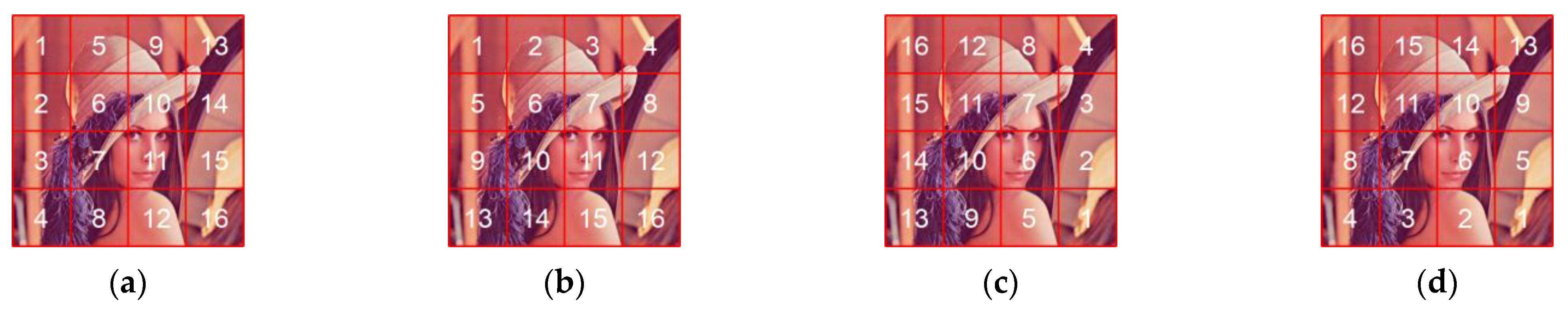
By default, the patches in all of the above-mentioned sliding methods are saved in a column-wise order. However, this can be changed using the Order parameter, with four possible values, namely column, row, columnrev, and rowrev. Figure 5 demonstrates this functionality. This parameter defines the order in which the patches are saved either as image files, as a MATLAB .mat file, or as raw text files. It should be noted that the parameter Order affects only patches created in sliding mode. In random mode, the order of patches is randomly defined by default.
3. Further Operations and Functionality
Aside from the basic patch operations regarding the creation and saving of patches, the patchIT tool supports further functionality that may be beneficial for certain patch-based image processing applications. This section introduces masking operations, as well as geometric transformations through patch value indexing, in addition to demonstrating how the patchIT tool efficiently handles memory issues in large-scale patch processing scenarios.
3.1. Masking Image Regions
In addition to the source image, a mask array can be also provided, acting as a spatial filter that affects the patch creation process. A masking process can be applied in cases in which certain image parts should be excluded from the candidate patch areas. From another point of view, a mask could also be used as a weighting array that provides significance information at the pixel level. A mask array should have dimensions equal to the source image itself and can be provided either as a MATLAB array or as an image file using the mask parameter. For instance, the commands
M=imread(‘sample512_mask.tif’);
patchit(‘sample512.jpg’,[32 32],’Mask’,M);
are equivalent to
patchit(‘sample512.jpg’,[32 32],’Mask’,’sample512_mask.tif’);
In the first case, the mask image file is imported into a MATLAB variable (M); then, this variable is used as a Mask parameter value. In the second approach, the mask file is directly imported to the patchIT tool. Both cases have their advantages. Providing the mask as a MATLAB variable offers increased flexibility, as the mask can be programmatically generated and/or modified before being imported into patchIT. On the other hand, an image-like visual representation of the mask may be the output of some external preprocessing step and is, in general, easier to interpret. Figure 6 demonstrates the masking results of the above-mentioned commands. On the left, the original 512 × 512 pixel image is shown superimposed with blue dots that denote the candidate patch positions. The mask shown in the middle is a binary image with the same dimensions as the source image. Only candidate patches that fit in the white areas are allowed, and all the others are filtered out. On the right side, the final extracted patches are shown over the source image.
It should be noted that in sliding mode, the mask values are treated in a two-state fashion. That is, any non-zero value is considered 1, leading to a binary representation of the mask.
In random mode, the mask (M) has a different interpretation. The mask is no longer binary but is considered a probability array denoting image areas that are favorable for patch extraction. Thus, the majority of the random patches is extracted from image locations where the corresponding mask values are high. For instance, Figure 7 depicts the results of the command
patchit(‘sample512.jpg’,[32 32],’Count’,15,’Mode’,’Random’,…
‘RandomMaxOverlap’,0, ‘Mask’,’sample512_maskgray.jpg’);
which asks for 15 non-overlapping random patches with dimensions of 32 × 32 based on a probability mask that is provided by the grayscale file sample512_maskgray.jpg.
Figure 7.
Applying a mask in random mode: (a) the source image; (b) a probability mask and 15 non-overlapping patches located in high-probability areas; (c) the resulting extracted patches.
Figure 7.
Applying a mask in random mode: (a) the source image; (b) a probability mask and 15 non-overlapping patches located in high-probability areas; (c) the resulting extracted patches.

3.2. Patch Indexing and Geometric Transformations
Patches are represented by their intensity values across all the bands of the source image. Especially when saved in .mat or raw (text) format, these values are easily accessible by the user, as they are provided either in a matrix form (.mat file) or in a row of values (raw text files). By default, indexing of these values is column-wise, as shown in Figure 4. The patchIT tool offers further functionality for the maintenance of patch intensity values, leading to the creation of various visual results. For example, each patch can be flipped upside down, mirrored left–right, swapped along the diagonal, rotated, etc. The parameter PatchIndexing controls this behavior, with various possible values that are detailed in Table 4. A sample 3 × 3 patch with values is used for demonstration. The default indexing is , which is column-based and can be modified by the PatchIndexing parameter, resulting in modified patch values.
For example, in the command
patchit(‘sample512.jpg’,[128 128],’SaveMode’,’images’,…
‘PatchIndexing’,’mirror’);
the mirror value is applied; thus, the 16 patches (shown originally in Figure 2a) are saved as horizontally flipped PNG images. It should be mentioned that multiple PatchIndexing values can be combined, resulting in an increased number of geometric transformations. Table 5 demonstrates various simple and combined PatchIndexing operations when applied to the 11th patch shown in Figure 5a.
Obviously, there is no visual interpretation for patches indexed using the spiralout or spiralin options. However, they provide a useful insight on patch intensities, especially when arranged in row vectors, as provided by raw saving mode. Figure 8 depicts an example in which 16 patches with dimensions of 5 × 5 pixels are indexed according to the spiralout option and the results are provided in raw format, i.e., one row per patch. Specifically, for each patch, the row representation starts with the inner pixel, followed by the eight pixels around it in clockwise direction, which are followed by 16 additional intensity values of the external pixels. Overall, a table is constructed based on all the patch intensities, providing a convenient way to process such inner-to-outer values. The first column of the table consists of the center pixel of all patches, and the next eight columns of the table consist of the surrounding pixels of all patches, etc. Similar compact representations regarding outer-to-inner intensities can be obtained by the spiralin option of the PatchIndexing parameter. This process is readily extended to multispectral images by considering the raw text files that correspond to the other bands. It should be noted that both spiral options are available only for square-shaped patches.
3.3. Processing Modes
As already mentioned, the number of created patches is a combination of various parameters that affect the workload both in terms of memory and time requirements. As shown in Table 1 and Table 2, it is fairly easy to exceed the system memory and to reach the maximum of the processor’s capabilities. The patchIT tool provides a parameter named ProcessingMode that controls how the tool operates in order to overcome the aforementioned difficulties. This parameter has two possible values, namely direct and block. The first option is the default, for which the requested patch extraction computations refer to the entire procedure as a whole. This approach is the faster of the two and is the appropriate choice for most typical applications. However, in large-scale scenarios (e.g., a combination of large images/large patch sizes/small stride values), an increasing amount of memory is required, which may render the extraction of patches infeasible. In this case, the block option can be used, which splits the process into smaller parts that use a fraction of the available memory, permitting unobstructed patch extraction, even in very large-scale scenarios. However, this approach is slower than the first one. Thus, the ProcessingMode parameter can be seen as a trade-off between efficiency and stability.
Table 6 demonstrates time and memory requirements in a 6 Core AMD Ryzen 5 3600 Processor @3.60 GHz with 16 GB of RAM when applied to an RGB color image with dimensions of 512 × 512 pixels. The patch size is set to 128 × 128, and the stride varies from (128,128) pixels, which results in dense, non-overlapping patches, to (1,1), which corresponds to one pixel sliding in both directions. It can be observed that the memory requirements increase rapidly, along with the number of patches. In all cases, saving to a .mat file is the fastest option. For large stride values, the two processing modes, i.e., direct and block, offer similar timings. On the other hand, the one-pixel sliding case is not feasible in direct mode due to memory limitations, whereas the block processing mode still provides a reliable solution.
4. Experimental Results of a Use Case in Cartographic Research
In this section, we effectively utilize the capabilities of the patchIT toolbox in order to address an issue in the field of cartography and mapping. The use case involves the execution of the introduced toolbox for the automatic generation of image patches using cartographic backgrounds characterized by different scale levels. The aforementioned process is vital for investigating map visual heterogeneity, which can be used as an indicator of map visual complexity. In particular, the described scenario examines the hypothesis that map visual heterogeneity is affected by map scale level. Shannon entropy is utilized as an indicator of visual heterogeneity.
The implementation of the use case is based on the utilization of the dataset described in a recent study [27]. The dataset involves 100 different maps (cartographic backgrounds) characterized by five different map scale levels (1:k, 1:2 k, 1:4 k, 1:10 k, and 1:40 k) in twenty different regions in Greece and was produced using the standard layer of OpenStreetMap (OSM). The resolution of each image corresponds to 2000 × 2000 px. This dataset is a subset of the corresponding dataset introduced by Kesidis et al. [28].
The experiments are performed in two stages. During the first stage, patchIT is executed for the automatic extraction of different patches from all images of the selected dataset using the random mode. Three different patch sizes (50 × 50 px, 100 × 100 px, and 200 × 200 px) and three different numbers (100, 200, and 500) of patches are randomly extracted all over the image by setting the patchIT parameter Mode to random and the parameter Count to 100, 200, and 500, respectively. The maximum percentage of allowed overlap is defined by setting the parameter RandomMaxOverlap to a value of 1 (any patch position and overlap is allowed). Figure 9 depicts an example in which the first 20 random patches are shown in the case of a 100 × 100 px patch size for a selected image (map) from the dataset.
Additionally, all patches are extracted in three different file formats (*.png image files, MATLAB *.mat file, and raw *.txt files) in order to evaluate the computation time requirements per processed image. Table 7 demonstrates the average time requirements of all dataset images with a 6 Core AMD Ryzen 5 3600 Processor @3.60 GHz with 16 GB of RAM for different patch sizes and saving modes.
The output from the first stage can be used to compute specific indicators for the quantification of visual heterogeneity that characterizes each (map) image based on the selected patches. Hence, in the second stage, Shannon entropy is derived from the patches of each image (patch-based entropy) as an indicator for every map in order to evaluate the effect of map scale on map visual complexity. Patch-based entropy is estimated for the case of a 100 × 100 px patch size and 200 samples of patches per image, similar to [27]. Specifically, the indicator is calculated based on the probability of observing similar mean RGB values in the 200 samples (patches) of each map (image). In order to evaluate the efficiency of the proposed patch-based entropy indicator, box plots are utilized, as shown in Figure 10. It is evident that scale level significantly affects the visual heterogeneity of maps, as decreasing the map scale level results in increased median values of the indicator.
In the above use case, the patchIT tool is applied to a large-scale image dataset in order to automatically produce randomly distributed samples; as shown in Table 7, the performed task is executed efficiently. Considering the functionality provided by the tool, it would be easy to change the patch sampling method from random to systematic by changing the Mode parameter from ‘Random’ to ‘Sliding’, allowing for a grid-like or even a dense, non-overlapping patch creation process, as depicted in Figure 2.
5. Discussion
The functionality provided by the patchIT tool is designed to facilitate the implementation of patch-oriented operations. Indeed, the combination of patch creation modes (sliding and random), image region masking, and patch indexing operations provides the potential to implement a wide spectrum of tasks in various domains.
One of the basic strengths of the tool is its suitability for spatial sampling, which is used to describe the activity of sampling when the population is spatially or geographically distributed by obtaining representative spatial attribute data from the population [29,30,31]. The PatchIT tool, through its provided functionalities of random and sliding modes for patch creation, along with region image masking with varying parameter values (e.g., Count, Stride, Mask) can facilitate various spatial sampling methods. In this sense, the most important methods of spatial sampling methods, namely (i) simple random spatial sampling, (ii) systematic spatial sampling, and (iii) stratified random spatial sampling [30,32,33], can be efficiently supported. Specifically, simple random spatial sampling can be enabled by patch creation in random mode (as presented in the Experimental Results section), systematic spatial sampling is supported by patch creation in sliding mode, and the combination of patch creation in random mode with properly formed region image masking can utilize stratified random spatial sampling. The latter method can be particularly useful when there are regions within a georeferenced image (e.g., remote sensing image) or a map, and it is essential that the attributes of these regions are sampled. For instance, in geographic regions where there are water bodies (e.g., lakes) that are prone to be severely contaminated and should not be omitted from the sampling procedure [29], the stratified random spatial sampling method is often suggested. In this context, recent research studies employed several spatial sampling methods and designs to capture spatial and temporal water quality variations in a lake environment utilizing remote sensing data [34].
Another domain in which the functionalities of the tool can be particularly useful is image denoising. Local denoising methods can be limited in images in which the correlations of neighboring pixels are greatly disturbed by high-level noise, mainly because such images contain extensive similar patches at different locations [35]. Techniques such as non-local means (NLM) based on a non-local averaging of all pixels in the image [36] aid in overcoming certain denoising limitations. In essence, NLM is a patch-based filter dividing the input image into sub-images in order to filter each sub-image separately (in a patch-wise manner) [37]. The algorithm for this filter is based on similarity comparisons, e.g., Euclidean distance between the centers of the patches and/or luminance distance between the patches of each sub-image within a search window. In this context, patches with similar luminance levels contribute with higher weights when averaged [37]. NLM is based on patch similarity comparisons, and the value of each estimated pixel occurs as a weighted average of pixels in the search window. Therefore, patch creation operations and patch indexing provided by patchIT can be of great use for image denoising. In particular, spiralout patch indexing can be harnessed, enabling comparisons in the vicinity, i.e., the surrounding pixels (one-pixel distant neighbors, two pixels distant neighbors, etc.) of pixels all over the image.
The proposed tool was developed with MATLAB software. Hence, the tool can be executed in all modern operating systems, including Windows, Mac OS, and various Linux distributions, if MATLAB is installed. Moreover, all the functionalities of the tool are fully supported by only one function and can be imported in any other MATLAB software, working either in a command line environment or in a graphical user interface (GUI).
6. Conclusions
PatchIT constitutes an integrated framework that serves as a complete software tool towards automatized patch creation processes. It offers extended functionality regarding the creation of patches in both a sliding and random manner that can be exported either as images, MATLAB .mat files, or raw text files. Patch creation can be further refined by involving masking techniques that act as spatial filters identifying candidate patch areas. Moreover, geometric transformations at the patch level are also provided by applying patch value indexing. The patchIT tool efficiently handles memory issues that arise in large-scale patch processing scenarios. It can be applied to all common image file formats and supports bitonal, grayscale, color, and multispectral images.
The applicability of the tool is demonstrated in a realistic scenario in which a large dataset of cartographic backgrounds is used to estimate visual heterogeneity with a patch-based entropy indicator. The patchIT tool follows an “easy-to-use” and “easy-to-adapt” approach that can be fully incorporated into applications and adjusted according to the particular user requirements. The source code of the tool is freely distributed to the scientific community under the third version of the GNU General Public License (GPL v3) on the GitHub platform (Supplementary Materials, https://github.com/taskes11/patchIT, accessed on 9 November 2022), providing the opportunity to perform any modification for further extension and development.
Supplementary Materials
Author Contributions
Conceptualization, A.L.K., V.K., L.-M.M. and N.M.; methodology, A.L.K., V.K., L.-M.M. and N.M.; software development, testing, and validation, A.L.K. and N.M.; investigation, A.L.K., V.K., L.-M.M. and N.M.; writing—original draft preparation, A.L.K.; writing—review and editing, A.L.K., V.K., L.-M.M. and N.M.; visualization, A.L.K. and V.K. All authors have read and agreed to the published version of the manuscript.
Funding
This research received no external funding.
Institutional Review Board Statement
Not applicable.
Informed Consent Statement
Not applicable.
Data Availability Statement
Not applicable.
Conflicts of Interest
The authors declare no conflict of interest.
References
- Dabov, K.; Foi, A.; Katkovnik, V.; Egiazarian, K. Image Denoising by Sparse 3-D Transform-Domain Collaborative Filtering. IEEE Trans. Image Process. 2007, 16, 2080–2095. [Google Scholar] [CrossRef] [PubMed]
- Qian, Y.; Shen, Y.; Ye, M.; Wang, Q. 3-D Nonlocal Means Filter with Noise Estimation for Hyperspectral Imagery Denoising. In International Geoscience and Remote Sensing Symposium (IGARSS); IEEE: Munich, Germany, 2012; pp. 1345–1348. [Google Scholar] [CrossRef]
- Papyan, V.; Elad, M. Multi-Scale Patch-Based Image Restoration. IEEE Trans. Image Process. 2016, 25, 249–261. [Google Scholar] [CrossRef]
- Liu, B.; Du, S.; Du, S.; Zhang, X. Incorporating Deep Features into GEOBIA Paradigm for Remote Sensing Imagery Classification: A Patch-Based Approach. Remote Sens. 2020, 12, 3007. [Google Scholar] [CrossRef]
- Sharma, A.; Liu, X.; Yang, X. Land Cover Classification from Multi-Temporal, Multi-Spectral Remotely Sensed Imagery Using Patch-Based Recurrent Neural Networks. Neural Netw. 2018, 105, 346–355. [Google Scholar] [CrossRef] [PubMed] [Green Version]
- Liu, Y.; Ren, Q.; Geng, J.; Ding, M.; Li, J. Efficient Patch-Wise Semantic Segmentation for Large-Scale Remote Sensing Images. Sensors 2018, 18, 3232. [Google Scholar] [CrossRef] [PubMed] [Green Version]
- Song, H.; Kim, Y.; Kim, Y. A Patch-Based Light Convolutional Neural Network for Land-Cover Mapping Using Landsat-8 Images. Remote Sens. 2019, 11, 114. [Google Scholar] [CrossRef] [Green Version]
- Cordier, N.; Delingette, H.; Ayache, N. A Patch-Based Approach for the Segmentation of Pathologies: Application to Glioma Labelling. IEEE Trans. Med. Imaging 2016, 35, 1066–1076. [Google Scholar] [CrossRef] [Green Version]
- Khawaja, A.; Khan, T.M.; Naveed, K.; Naqvi, S.S.; Rehman, N.U.; Junaid Nawaz, S. An Improved Retinal Vessel Segmentation Framework Using Frangi Filter Coupled with the Probabilistic Patch Based Denoiser. IEEE Access 2019, 7, 164344–164361. [Google Scholar] [CrossRef]
- Bustin, A.; Lima da Cruz, G.; Jaubert, O.; Lopez, K.; Botnar, R.M.; Prieto, C. High-Dimensionality Undersampled Patch-Based Reconstruction (HD-PROST) for Accelerated Multi-Contrast MRI. Magn. Reson. Med. 2019, 81, 3705–3719. [Google Scholar] [CrossRef]
- Bernal, J.; Kushibar, K.; Cabezas, M.; Valverde, S.; Oliver, A.; Llado, X. Quantitative Analysis of Patch-Based Fully Convolutional Neural Networks for Tissue Segmentation on Brain Magnetic Resonance Imaging. IEEE Access 2019, 7, 89986–90002. [Google Scholar] [CrossRef]
- Manjón, J.V.; Coupe, P. MRI Denoising Using Deep Learning. In Lecture Notes in Computer Science (Including Subseries Lecture Notes in Artificial Intelligence and Lecture Notes in Bioinformatics); Springer: Cham, Switzerland, 2018; pp. 12–19. [Google Scholar] [CrossRef]
- Nasor, M.; Obaid, W. Detection and Localization of Early-Stage Multiple Brain Tumors Using a Hybrid Technique of Patch-Based Processing, k-Means Clustering and Object Counting. Int. J. Biomed. Imaging 2020, 2020, 1–8. [Google Scholar] [CrossRef] [PubMed] [Green Version]
- Pérez-García, F.; Sparks, R.; Ourselin, S. TorchIO: A Python Library for Efficient Loading, Preprocessing, Augmentation and Patch-Based Sampling of Medical Images in Deep Learning. Comput. Methods Programs Biomed. 2021, 208, 106236. [Google Scholar] [CrossRef] [PubMed]
- Barnes, C.; Zhang, F.L. A Survey of the State-of-the-Art in Patch-Based Synthesis. Comput. Vis. Media 2017, 3, 3–20. [Google Scholar] [CrossRef] [Green Version]
- Zhang, R.; Yi, X.; Li, H.; Liu, L.; Lu, G.; Chen, Y.; Guo, X. Multiresolution Patch-Based Dense Reconstruction Integrating Multiview Images and Laser Point Cloud. Int. Arch. Photogramm. Remote Sens. Spat. Inf. Sci. 2022, XLIII-B2-2, 153–159. [Google Scholar] [CrossRef]
- Shen, S. Accurate Multiple View 3D Reconstruction Using Patch-Based Stereo for Large-Scale Scenes. IEEE Trans. Image Process. 2013, 22, 1901–1914. [Google Scholar] [CrossRef]
- Minoura, H.; Yonetani, R.; Nishimura, M.; Ushiku, Y. Crowd Density Forecasting by Modeling Patch-Based Dynamics. IEEE Robot. Autom. Lett. 2021, 6, 287–294. [Google Scholar] [CrossRef]
- Kentsch, S.; Caceres, M.L.L.; Serrano, D.; Roure, F.; Diez, Y. Computer Vision and Deep Learning Techniques for the Analysis of Drone-Acquired Forest Images, a Transfer Learning Study. Remote Sens. 2020, 12, 1287. [Google Scholar] [CrossRef] [Green Version]
- Mirzaalian, H.; Hussein, M.; Abd-Almageed, W. On the Effectiveness of Laser Speckle Contrast Imaging and Deep Neural Networks for Detecting Known and Unknown Fingerprint Presentation Attacks. In Proceedings of the 2019 International Conference on Biometrics (ICB), Crete, Greece, 4–7 June 2019. [Google Scholar] [CrossRef]
- MacEachren, A.M. Map Complexity: Comparison and Measurement. Am. Cartogr. 1982, 9, 31–46. [Google Scholar] [CrossRef]
- Fairbairn, D. Measuring Map Complexity. Cartogr. J. 2006, 43, 224–238. [Google Scholar] [CrossRef]
- Schnur, S.; Bektaş, K.; Çöltekin, A. Measured and Perceived Visual Complexity: A Comparative Study among Three Online Map Providers. Cartogr. Geogr. Inf. Sci. 2017, 45, 238–254. [Google Scholar] [CrossRef]
- Liao, H.; Wang, X.; Dong, W.; Meng, L. Measuring the Influence of Map Label Density on Perceived Complexity: A User Study Using Eye Tracking. Cartogr. Geogr. Inf. Sci. 2018, 46, 210–227. [Google Scholar] [CrossRef]
- Tzelepis, N.; Kaliakouda, A.; Krassanakis, V.; Misthos, L.M.; Nakos, B. Evaluating the Perceived Visual Complexity of Multidirectional Hill-Shading. Geod. Cartogr. 2020, 69, 161–172. [Google Scholar]
- Keil, J.; Edler, D.; Kuchinke, L.; Dickmann, F. Effects of Visual Map Complexity on the Attentional Processing of Landmarks. PLoS ONE 2020, 15, e0229575. [Google Scholar] [CrossRef] [PubMed] [Green Version]
- Merlemis, N.; Kesidis, A.; Misthos, L.-M.; Zekou, E.; Drakaki, E.; Krassanakis, V. Quantifying Visual Heterogeneity of Paper Maps Using Diffuse Reflectance Spectroscopy. Abstr. ICA 2022, 5, 1–2. [Google Scholar] [CrossRef]
- Kesidis, A.L.; Krassanakis, V.; Merlemis, N.; Misthos, L.-M. A Multipurpose Patch Creation Tool for Efficient Exploration of Digital Cartographic Products. Abstr. ICA 2022, 5, 1–2. [Google Scholar] [CrossRef]
- Haining, R. Spatial Data Analysis: Theory and Practice. Spat. Data Anal. 2003. [Google Scholar] [CrossRef]
- Delmelle, E.M. Spatial Sampling. Handb. Reg. Sci. 2014, 1385–1399. [Google Scholar] [CrossRef]
- Haining, R.P. Spatial Sampling. Int. Encycl. Soc. Behav. Sci. 2001, 14822–14827. [Google Scholar] [CrossRef]
- Brus, D.J.; Knotters, M. Sampling Design for Compliance Monitoring of Surface Water Quality: A Case Study in a Polder Area. Water Resour Res 2008, 44. [Google Scholar] [CrossRef] [Green Version]
- Wang, J.F.; Stein, A.; Gao, B.B.; Ge, Y. A Review of Spatial Sampling. Spat Stat 2012, 2, 1–14. [Google Scholar] [CrossRef]
- Li, J.; Tian, L.; Wang, Y.; Jin, S.; Li, T.; Hou, X. Optimal Sampling Strategy of Water Quality Monitoring at High Dynamic Lakes: A Remote Sensing and Spatial Simulated Annealing Integrated Approach. Sci. Total Environ. 2021, 777, 146113. [Google Scholar] [CrossRef]
- Fan, L.; Zhang, F.; Fan, H.; Zhang, C. Brief Review of Image Denoising Techniques. Vis. Comput. Ind. 2019, 2, 7. [Google Scholar] [CrossRef] [PubMed] [Green Version]
- Buades, A.; Coll, B.; Morel, J.M. A Non-Local Algorithm for Image Denoising. In Proceedings of the 2005 IEEE Computer Society Conference on Computer Vision and Pattern Recognition, CVPR 2005, San Diego, CA, USA, 20–25 June 2005; Volume II, pp. 60–65. [Google Scholar] [CrossRef]
- Alkinani, M.H.; El-Sakka, M.R. Patch-Based Models and Algorithms for Image Denoising: A Comparative Review between Patch-Based Images Denoising Methods for Additive Noise Reduction. EURASIP J. Image Video Process. 2017, 2017, 58. [Google Scholar] [CrossRef] [PubMed]
Figure 1.
Patch extraction examples for various image types (a) in a monochromatic image, (b) in a color (RGB) image, and (c) in a multispectral image.
Figure 1.
Patch extraction examples for various image types (a) in a monochromatic image, (b) in a color (RGB) image, and (c) in a multispectral image.

Figure 3.
Creating random patches: (a) 15 patches with dimensions of 64 × 64 randomly positioned all over the source image (overlapping of patches is allowed); (b) 5 patches with dimensions of 128 × 128 randomly positioned all over the source image (overlapping of patches is allowed for up to 10% of the patch’s area, and a maximum of 50 attempts is allowed in order to find patches that fulfill the requested conditions).

Figure 4.
Demo example depicting (left) the first two (out of N) patches with dimensions of 3 × 3 of an example color RGB image and (right) the first two lines of the corresponding raw text files. Each text file line contains 3 × 3 = 9 values, and there are as many lines as the number (N) of patches.

Figure 5.
The four options for the Order parameter for patches created in sliding mode: (a) column (default), (b) row, (c) columnrev, and (d) rowrev.
Figure 5.
The four options for the Order parameter for patches created in sliding mode: (a) column (default), (b) row, (c) columnrev, and (d) rowrev.

Figure 6.
Applying a mask in sliding mode: (a) source image with the candidate patch positions marked with blue dots; (b) a binary mask with the patches that fit in the white (allowed) areas; (c) the resulting extracted patches.
Figure 6.
Applying a mask in sliding mode: (a) source image with the candidate patch positions marked with blue dots; (b) a binary mask with the patches that fit in the white (allowed) areas; (c) the resulting extracted patches.

Figure 8.
Representation of 16 patches with 25 intensity values per patch. The spiralout option of the PatchIndexing parameter starts from the innermost pixel and gradually extends to the outer pixels of the patch in a clockwise direction. The patch pixels are indexed in squares of increasing distance from patch center.

Figure 9.
Illustration of the first 20 randomly generated patches on a selected map (2000 px resolution; map scale level, 1:10 k). The patches shown have dimensions 100 × 100 and are randomly positioned all over the map image, and full overlapping of patches is allowed.
Figure 9.
Illustration of the first 20 randomly generated patches on a selected map (2000 px resolution; map scale level, 1:10 k). The patches shown have dimensions 100 × 100 and are randomly positioned all over the map image, and full overlapping of patches is allowed.

Figure 10.
Box plots of the patch-based entropy for 100 sample images at five different scale levels. The red mark corresponds to the median, and the bottom and top edges indicate the 25th and 75th percentiles, respectively. The whiskers indicate extreme data points, and the outliers are denoted by a red cross symbol. The indicator is estimated based on probability of observing different mean RGB values for the 200 patches that are randomly generated with patchIT for each image (map).


Table 1.
Overall number of patches for various stride and patch sizes in a medium-sized image (512 × 512 pixels) and a 4K image (3840 × 2160 pixels).
Table 1.
Overall number of patches for various stride and patch sizes in a medium-sized image (512 × 512 pixels) and a 4K image (3840 × 2160 pixels).
| Stride | (128,128) | 16 | 16 | 16 | 480 | 510 | 510 |
| (64,64) | 49 | 64 | 64 | 1888 | 2040 | 2040 | |
| (16,16) | 625 | 961 | 1024 | 29,824 | 32,026 | 32,400 | |
| (4,4) | 9409 | 14,641 | 16,129 | 472,861 | 507,949 | 516,901 | |
| (1,1) | 148,225 | 231,361 | 255,025 | 7,548,529 | 8,109,361 | 8,252,449 | |
Table 2.
Memory requirements (in megabytes, MB) assuming 1 byte/pixel for various stride and patch sizes when applied to two monochromatic images () with dimensions of 512 × 512 and 3840 × 2160 pixels, respectively.
Table 2.
Memory requirements (in megabytes, MB) assuming 1 byte/pixel for various stride and patch sizes when applied to two monochromatic images () with dimensions of 512 × 512 and 3840 × 2160 pixels, respectively.
| Stride | (128,128) | 0.250 | 0.016 | 0.001 | 7.500 | 0.498 | 0.031 |
| (64,64) | 0.766 | 0.062 | 0.004 | 29.500 | 1.992 | 0.125 | |
| (16,16) | 9.766 | 0.938 | 0.062 | 466.000 | 31.275 | 1.978 | |
| (4,4) | 147.016 | 14.298 | 0.984 | 7388.453 | 496.044 | 31.549 | |
| (1,1) | 2316.016 | 225.938 | 15.565 | 11,7945.766 | 7919.298 | 503.690 | |
Table 3.
Patch-saving options.
| Saving Mode | Description | Example |
|---|---|---|
| images | Saves patches into separate image files | patchit(‘image.jpg’,[128 128],… ‘Stride’,[64 64],’SaveMode’,’images’,… ‘SaveImagesTemplate’,’C:\results\patchfile000.png’); Creates PNG patch files with dimensions of 128 × 128 in folder C:\results using the filename template patchfile000 as ‘C:\results\patchfile001.png’ ‘C:\results\patchfile002.png’ … (etc) … |
| mat | Saves all patches into a multidimensional variable | patchit(‘image.jpg’,[32 32],… ‘Stride’,[4 4],’SaveMode’,’mat’,… ‘SaveMatFilename’,’C:\results\allpatches.mat’); Creates file allpatches.mat in folder C:\results that contains all the 32 × 32 patches |
| raw | Save intensity values into separate text files—one per spectral band | patchit(‘image.jpg’,[15 15],… ‘Stride’,[64 64],’SaveMode’,’raw’,… ‘SaveRawFilename’,’C:\results\rawdata.txt’); Creates a separate text file (one per each spectral band) in folder C:\results. Assuming that ‘image.jpg’ is a multispectral image with eight bands, the following eight text files are created: ‘C:\results\rawdata1.txt’ ‘C:\results\rawdata2.txt’ … ‘C:\results\rawdata8.txt’ corresponding to intensity values for each spectral band. |
Table 4.
Patch indexing operations.
| Patch Indexing Value | Description | Indexing Example | Patch Values Example |
|---|---|---|---|
| default | no change | 1 4 7 1 4 7 2 5 8 → 2 5 8 3 6 9 3 6 9 | 124 128 133 124 128 133 143 143 140 → 143 143 140 159 158 151 159 158 151 |
| mirror | horizontal flip | 1 4 7 7 4 1 2 5 8 → 8 5 2 3 6 9 9 6 3 | 124 128 133 133 128 124 143 143 140 → 140 143 143 159 158 151 151 158 159 |
| flip | vertical flip | 1 4 7 3 6 9 2 5 8 → 2 5 8 3 6 9 1 4 7 | 124 128 133 159 158 151 143 143 140 → 143 143 140 159 158 151 124 128 133 |
| swap | x-y exchange | 1 4 7 1 2 3 2 5 8 → 4 5 6 3 6 9 7 8 9 | 124 128 133 124 143 159 143 143 140 → 128 143 158 159 158 151 133 140 151 |
| spiralout | inner-to-outer spiral pattern | 1 4 7 7 8 9 2 5 8 → 6 1 2 3 6 9 5 4 3 | 124 128 133 143 158 124 143 143 140 → 140 159 128 159 158 151 151 143 133 |
| spiralin | outer-to-inner spiral pattern | 1 4 7 1 2 3 2 5 8 → 8 9 4 3 6 9 7 6 5 | 124 128 133 124 140 159 143 143 140 → 128 151 143 159 158 151 133 158 143 |
Table 5.
Examples of patch indexing operations when applied to a 128 × 128 patch.
| PatchIndexing Value | Resulting Patch | PatchIndexing Value | Resulting Patch |
|---|---|---|---|
| default |  | flip + swap (rotate 90° clockwise) |  |
| mirror |  | flip + mirror (rotate 180°) |  |
| flip |  | spiralout |  |
| swap |  | spiralin |  |
Table 6.
Time and memory requirements regarding an RGB color image with dimensions of 512 × 512 pixels and patch size set to 128 × 128 pixels.
Table 6.
Time and memory requirements regarding an RGB color image with dimensions of 512 × 512 pixels and patch size set to 128 × 128 pixels.
| Patch Dimensions (W × H) | Patches (N) | Memory (Bytes) | Time (s) | Time (s) | |||||
|---|---|---|---|---|---|---|---|---|---|
| Images | .Mat | Raw Files | |||||||
| Direct | Block | Direct | Block | Direct | Block | ||||
| 50 × 50 | 100 | 750,000 | 0.18 | 0.1 | 0.3 | 0.0 | 0.1 | 0.3 | 0.5 |
| 50 × 50 | 200 | 1,500,000 | 0.36 | 0.3 | 0.7 | 0.1 | 0.2 | 0.7 | 1.2 |
| 50 × 50 | 500 | 3,750,000 | 0.90 | 3.8 | 3.9 | 0.9 | 1.2 | 8.5 | 11.8 |
| 4 × 4 | 9409 | 462,471,168 | 57.5 | 57.9 | 13.7 | 15.5 | 124.6 | 215.1 | |
| 1 × 1 | 148,225 | 7,285,555,200 | - | 927.1 | - | 215.6 | - | 2077.4 | |
Table 7.
Average time requirements regarding the patch creation process for various combinations of patch number and size. All three output options are considered, namely saving the patches to image files, to a MATLAB .mat file, and to raw text files.
Table 7.
Average time requirements regarding the patch creation process for various combinations of patch number and size. All three output options are considered, namely saving the patches to image files, to a MATLAB .mat file, and to raw text files.
| Patch Dimensions (W × H) | Patches (N) | Time (s) | ||
|---|---|---|---|---|
| Images | .Mat | Raw Files | ||
| 50 × 50 | 100 | 0.18 | 0.03 | 0.22 |
| 50 × 50 | 200 | 0.36 | 0.04 | 0.44 |
| 50 × 50 | 500 | 0.90 | 0.07 | 1.04 |
| 100 × 100 | 100 | 0.25 | 0.06 | 0.91 |
| 100 × 100 | 200 | 0.49 | 0.10 | 1.76 |
| 100 × 100 | 500 | 1.20 | 0.22 | 4.27 |
| 200 × 200 | 100 | 0.49 | 0.21 | 4.37 |
| 200 × 200 | 200 | 1.01 | 0.46 | 8.53 |
| 200 × 200 | 500 | 2.61 | 0.79 | 21.00 |
Publisher’s Note: MDPI stays neutral with regard to jurisdictional claims in published maps and institutional affiliations. |
© 2022 by the authors. Licensee MDPI, Basel, Switzerland. This article is an open access article distributed under the terms and conditions of the Creative Commons Attribution (CC BY) license (https://creativecommons.org/licenses/by/4.0/).
Share and Cite
MDPI and ACS Style
Kesidis, A.L.; Krassanakis, V.; Misthos, L.-M.; Merlemis, N. patchIT: A Multipurpose Patch Creation Tool for Image Processing Applications. Multimodal Technol. Interact. 2022, 6, 111. https://doi.org/10.3390/mti6120111
AMA Style
Kesidis AL, Krassanakis V, Misthos L-M, Merlemis N. patchIT: A Multipurpose Patch Creation Tool for Image Processing Applications. Multimodal Technologies and Interaction. 2022; 6(12):111. https://doi.org/10.3390/mti6120111
Chicago/Turabian StyleKesidis, Anastasios L., Vassilios Krassanakis, Loukas-Moysis Misthos, and Nikolaos Merlemis. 2022. "patchIT: A Multipurpose Patch Creation Tool for Image Processing Applications" Multimodal Technologies and Interaction 6, no. 12: 111. https://doi.org/10.3390/mti6120111