Analysis of Vaneless Diffuser Stall Instability in a Centrifugal Compressor ^†

Abstract

Numerical simulations based on the large eddy simulation approach were conducted with the aim to explore vaneless diffuser rotating stall instability in a centrifugal compressor. The effect of the impeller blade passage was included as an inlet boundary condition with sufficiently low flow angle relative to the tangent to provoke the instability and cause circulation in the diffuser core flow. Flow quantities, velocity and pressure, were extracted to accumulate statistics for calculating mean velocity and mean Reynolds stresses in the wall-to-wall direction. The paper focuses on the assessment of the complex response of the system to the velocity perturbations imposed, the resulting pressure gradient and flow curvature effects.

1. Introduction

Ideally, for an efficient design the centrifugal compressor provides a steady fluid flow at an elevated pressure with minimal losses. However, the performance of the centrifugal compressor is harmed under the off-design operating conditions occurring at low flow rates. In such circumstances flow instabilities are developed through the compressor, which may cause large fluctuations in the flow variables and even introduce vibrations with high structural stress levels into the machine. This is an unwanted situation and the aim is therefore to understand the physical mechanisms responsible for the developed flow instabilities. Through linear stability analysis, see e.g., [1], the diffuser rotating stall is said to occur when the local return flow angle relative the meridional exceeds 90${}^{\circ }$. However, a diffuser instability generally develops earlier than 90${}^{\circ }$, i.e., prior to purely tangential flow. There exist some correlations that indicate the instability angle to be around 75${}^{\circ }$–85${}^{\circ }$ with respect to the radial direction depending on the operating conditions, see e.g., [2]. The theory [1] also states that it occurs with steady, uniform inflow and outflow conditions and thus independent of the interaction with the rotating impeller. A criticism is that inflow periodic unsteadiness may trigger a diffuser instability, see e.g., [3]. Another criticism is that the theory assumes diffuser flow as inviscid. This implies that the dynamic character of diffuser rotating stall depends on the inviscid core flow and is independent of viscous effects, dominating in the boundary layer. It is important to acknowledge some observations where the periodic unsteadiness may be delaying stall, see e.g., [4] where low pressure turbine suction side boundary layer stall, and axial compressor stall were investigated.

For the actual evolution of the dynamic character and thus prediction of the number of rotating stall cells and their propagation speed around the annulus, different research groups have considered a time-evolving calculation assuming 2D-unsteady, inviscid and incompressible flow, see e.g., [5,6,7]. The effect of the blades on the flow is fed at the diffuser inlet boundary and a Dirichlet condition with static pressure is considered on the outlet surface. One observation is that the evolution of the rotating stall cells depends on the specified outlet boundary condition; see e.g., [8]. Specification of a Dirichlet boundary condition at the outlet was seen to result in strong gradients of the velocity field. This is in contrast to the linear stability analysis where the Neumann boundary condition is used, which assumes zero pressure gradients in both the radial and tangential directions. In scenarios with reversing flow at the outlet boundary special consideration is needed for an appropriate specification of the backflow direction. This could be extrapolated or it could be treated as normal to the face elements on the outlet surface. In the ideal case, the outlet boundary would be extended further downstream to prevent recirculation. In the linear stability analysis work of [1], extrapolating the backflow direction was seen to be in agreement with experimental results of [9] for a wide vaneless diffuser with uniform inflow. The rotating stall feature was illustrated as two high static pressure cells at low velocity with reversing flow and two lower pressure cells at higher outgoing velocity. This was later confirmed in the 2D linear stability analysis by [5]. These cells were reported to be rotating at sub-synchronous rotational speed. In a real diffuser design the channel width is narrow where viscous effects in the boundary layer cannot be neglected. This is due to the growth of the displacement thickness that may be different on the wall boundaries, depending on the quality of the flow delivered by the impeller, see e.g., [10]. Additionally, the rotation of the impeller with high blade tip speed results in a high Reynolds number flow that enters the diffuser. Therefore the flow is thus turbulent with large fluctuations in the flow quantities, and subsequently with high shear rate, which may become unstable. Typically, the fluctuations are amplified at off-design conditions, as documented by [11]. These effects are not taken into account with the 2D inviscid approach. In the work by [12] the Navier–Stokes equations were averaged with the Reynolds decomposition resulting in the need for turbulence closure modeling. They employed a two equation isotropic turbulence model. The numerical result was found in good agreement with observed pressure fluctuations and number of rotating stall cells as compared with particle imaging velocimety (PIV), see [13]. However, it was concluded that the numerical result using isotropic turbulence modeling underestimates the strength of the rotating stall vortex as compared with PIV measurements. This may be explained by excessive turbulent diffusion, a known issue of linear turbulence models in presence of adverse pressure gradients, and issues associated with predicting accurately features such as boundary layer separation. Many different closure models exist for calculating turbulent flow. In the case of the diffuser flow there is evidently some argument for including curvature effects in the modeling approach, since curvature requires discerning turbulence anisotropy. Consequently, it is clear that the turbulence model should take anisotropic effects into consideration on top of considering an approach able to resolve the large, energy containing flow structures. Streamline-curvature is possible to include in the framework of eddy-viscosity turbulence modeling. For this, a correction factor is introduced to the turbulent production term in the turbulent kinetic energy equation, see e.g., [14]. This factor depends on the strain-rate as well as the rotation-rate tensor including several proposed modeling constants. Due to the large freedom in choosing the modeling constants a small variation to proposed default values may potentially yield significant differences in the predicted turbulence production. Nevertheless, eddy-viscosity modeling with curvature correction showed good predictive quality compared to experimental data for a vaneless diffuser application during rotating stall conditions, as shown in [15].

Previously it was demonstrated that the angular momentum instability associated with curvature plays a key role in provoking large effects on the turbulent boundary layer, see work by [16]. The boundary layer is affected by the radial pressure gradient, radial curvature near the inlet and tangential straining as the flow cross section area increases. Since the flow is swirling it is, therefore, necessary to include 3D effects and the destabilizing tangential curvature.

The present paper aims to capture the evolution of the rotating stall cells and their propagation around the annulus by employing the large eddy simulation (LES)-based approach to a 3D annular vaneless diffuser configuration with a turnaround outlet. The possibility of capturing anisotropic turbulence effect in the boundary layer will help elucidate the variation of velocities and Reynolds stresses in the swirling diffuser flow. Especially in key areas close to separation and recirculation in order to investigate the effect on fluctuation levels. For a statistical assessment the flow field is quantified by means of flow mode decomposition techniques. A sensitivity study to the outlet boundary conditions imposed will be carried out. The numerical methodology is described in the next section, which is followed by presentation of results. The relevance of the obtained results to the scientific and designer community is included in a concluding summary section.

2. Numerical Methodology

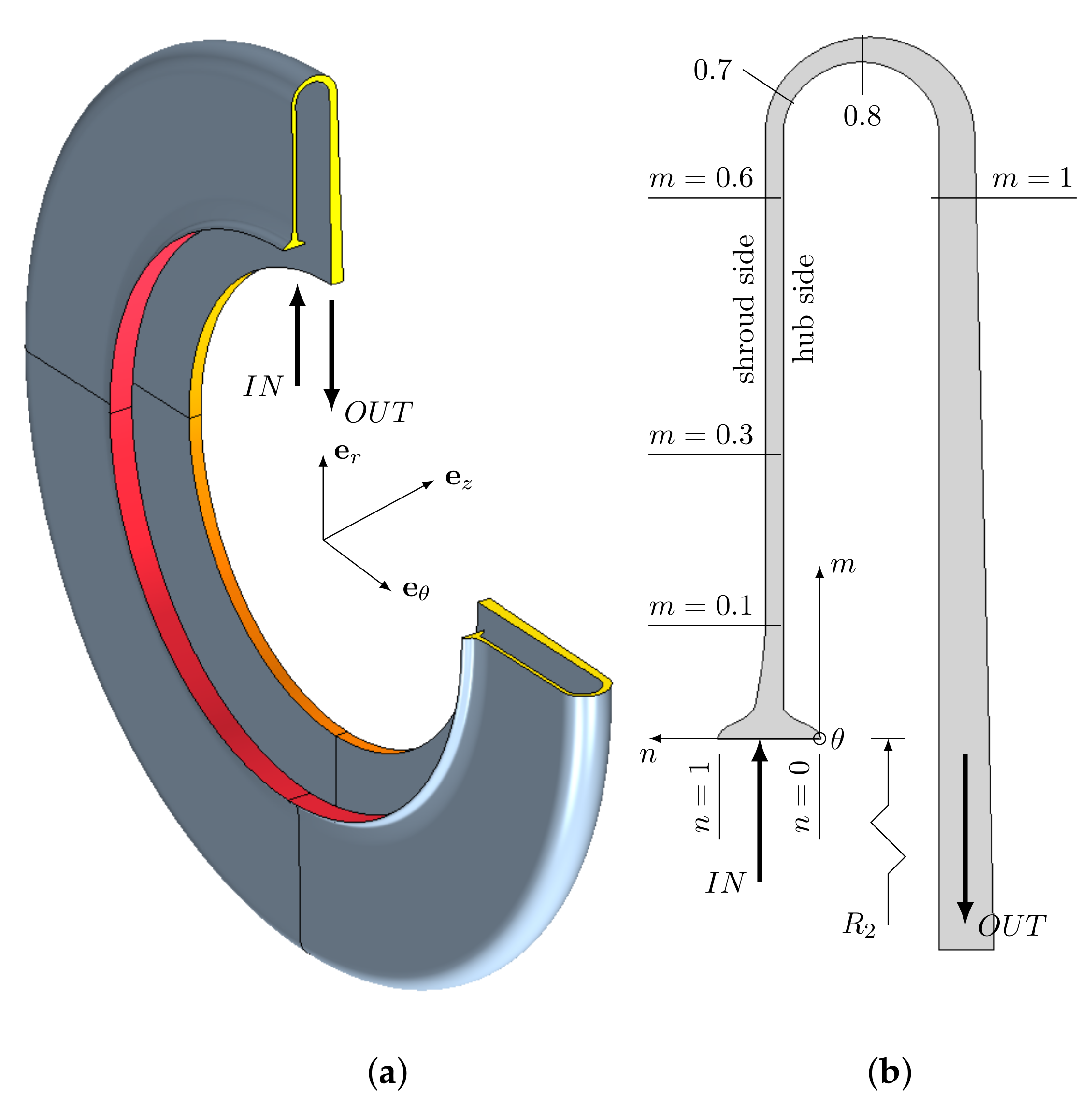
The narrow annular vaneless diffuser with a turnaround outlet, shown in Figure 1, contains a converging section close to the impeller blades. The overall extent before the turnaround in the radial direction is $\approx 1.5R_2$. The curvature of the turnaround is approximately $0.2R_2$ and the outlet is extruded to a location at $0.82R_2$.

The effect of the impeller blade passing is provided as meridional and tangential velocity profiles, respectively. The 3D time-dependent large-scale turbulent motion responsible for the fluid mixing in the vaneless diffuser is computed using the LES approach. The computational domain is discretized with a curvilinear grid which constitutes the elements of the finite volume methodology employed. Via Taylor series expansion an approximate representation is obtained for the transient, convective and diffusive terms respectively. The temporal term is discretized with a second order scheme, which uses the solution from the current time step and from the previous two time levels. A hybrid second order upwind/central differencing scheme is used for the convective term. The diffusive flux term is treated with a second-order expression, which involves the cell center value, the neighboring cell center value, and including the diffusion flux at the interior face. The introduced dissipative truncation error is known to mimic Smagorinsky-type SubGrid scale (SGS) modeling, see works by [17,18]. As the grid size is refined the filter size for SGS modeling subsequently decreases. Hence, the contribution from SGS may therefore become very small as compared to other entities in the momentum balance equation. One may therefore disregard from the SGS term by setting it to zero, which is attributed as implicit LES with no explicit SGS. The validity of an implicit LES approach can be verified by evaluating the energy decay slope for a point exhibiting isotropic turbulence in the inertial subrange, i.e., $-5/3$ for a velocity fluctuating component. However, such condition is not expected for a narrow channel flow under pressure gradient and strong flow curvature yielding significant effect on the boundary layer development and with associated separation. Therefore, code validation is assessed alternatively by means of a grid dependency study, which is presented further below. Nevertheless, the solver has been used previously for calculating flow scenarios associated with centrifugal compressors at low mass flow rates and validations against experimental data were carried out, see [19,20,21].

A constant-density turbulent flow is assumed with a Reynolds number $R{e}_b\approx 1\times {10}^5$ and inlet reference Mach number $M_{ref}=0.2$. The reference flow angle at the inlet boundary is relative to the tangential. It is computed in a point between the blades (i.e., $\theta /\chi =0.5$) and at the diffuser channel midpoint between the shroud and hub side (i.e., $n=0.5$):

$${\alpha }_{IN}=arctan(U_m/U_{\theta })$$

(1)

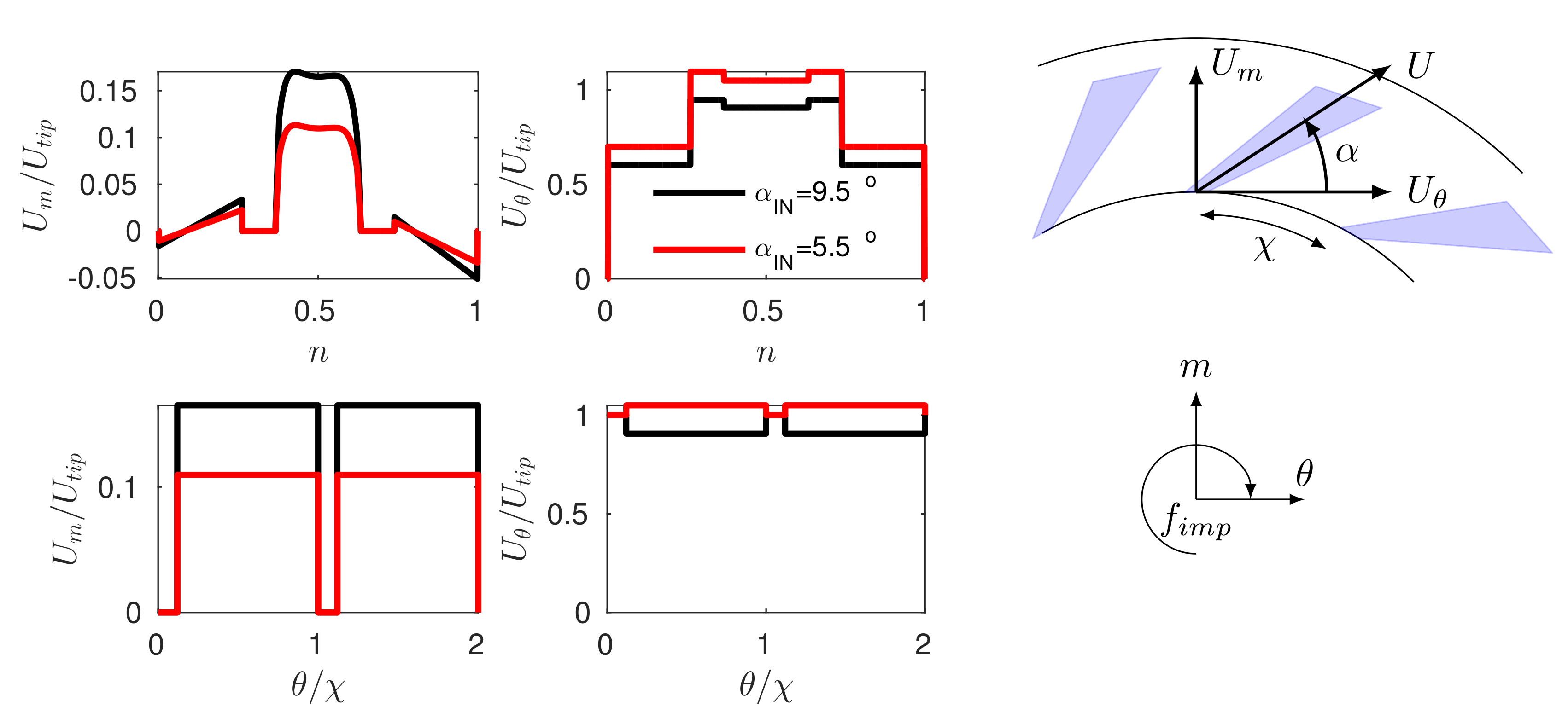
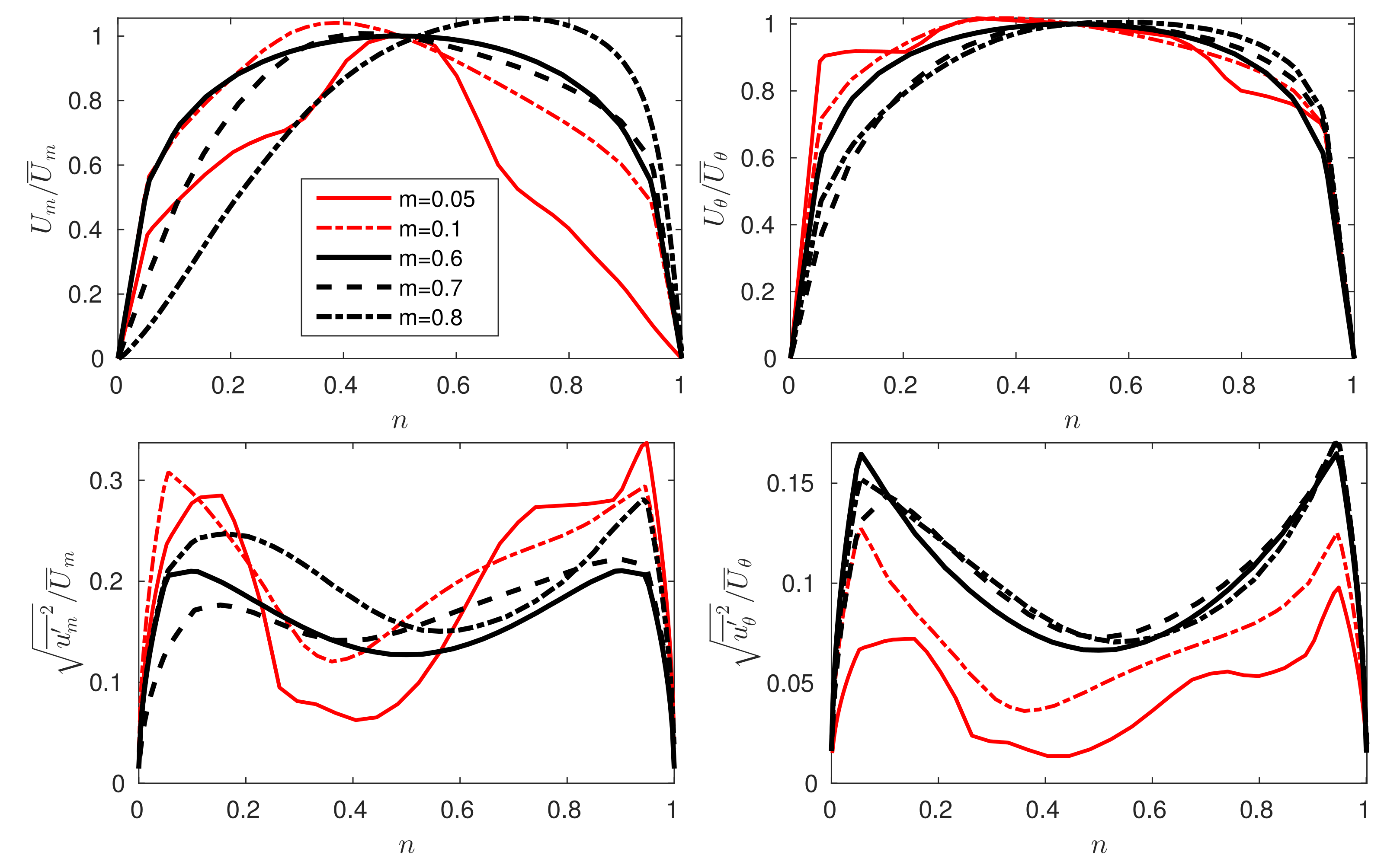
At the inlet boundary $U_m$ and $U_{\theta }$ have variable distributions in both axial and tangential directions, with purpose to mimic a real velocity distribution from an upstream impeller. Figure 2 shows the meridional and tangential velocity profile distributions scaled with $U_{tip}$ for two different reference inlet flow angle cases ${\alpha }_{IN}$ = 9.5${}^{\circ }$ and ${\alpha }_{IN}$ = 5.5${}^{\circ }$.

For each blade tip width segment circumferentially around the inlet diffuser plane, $U_{\theta }=U_{tip}$ and $U_m=0$. This has the effect of modeling the blade blockage effect, which is presented as tangential distributions for two blade passages, see last row in Figure 2 for orientation purposes. In addition, the velocity distribution is made to rotate at the impeller angular velocity $f_{IMP}$. Comparing peak values in Figure 2 it can be seen that the amplitude of the flow distortion entering the domain is in the order of $0.1U_{tip}$ at the distinct blade passing frequency $f_{BPF}$. Additional stochastic fluctuation is not considered, due to the overwhelming effect of the periodic unsteady incoming wakes described in Figure 2. At the outlet boundary, the pressure is fixed when the flow is outgoing. In case of backflow the pressure and flow direction is extrapolated from the outlet boundary. At the inlet the velocity components are specified and pressure is allowed to float. Therefore, the pressure is fixed in the scenario with pure outflow at the pressure outlet cell faces.

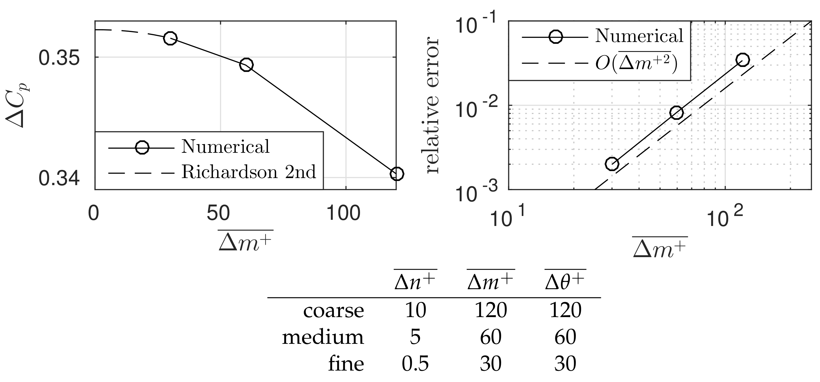
For validity of the numerical result a grid dependency study is performed on three different grids named; coarse, medium and fine (see also Figure 3). A grid refinement factor of two is used between grids. The wall resolution for the fine grid considered is: $\overline{\Delta n^{+}}=0.5$, $\overline{\Delta m^{+}}=30$, and $\overline{\Delta {\theta }^{+}}=30$. The normalized wall distances are computed as the surface average of the hub and shroud walls, respectively, between meridional stations $m=0$ and $m=1$. For a fair comparison the time-step size is adjusted between grids so that the time averaged convective Courant number is unity. Approximately 30 through flow times were simulated for each case. Five through flow times were needed to establish a suitable initial turbulent flow field. Therefore, data corresponding to 25 through flow times are used for statistical analysis of the flow field, which is adequate to capture a low frequency instability in the order of $0.02f_{BPF}$. The integrated pressure rise $\Delta C_p$ is computed as the difference in area averaged pressure coefficient at meridional stations $m=0$ and $m=0.8$, respectively. This parameter is evaluated with respect to the grid resolution in the meridional direction $\overline{\Delta m^{+}}$. Figure 3 indicates that the solution (i.e., $\Delta C_p$) approach an asymptotic limit value as the grid is refined. The Richardson 2nd order extrapolation shows that the fine grid resolution is marginally different compared to a hypothetical infinite grid resolution. It is also evident that the relative error with respect to the infinite grid solution drops monotonically two orders of magnitude for each refinement order. This result correlates with the chosen second order scheme and an expected truncation error of $O\left(\overline{\Delta m^{+2}}\right)$.

3. LES Data Analysis

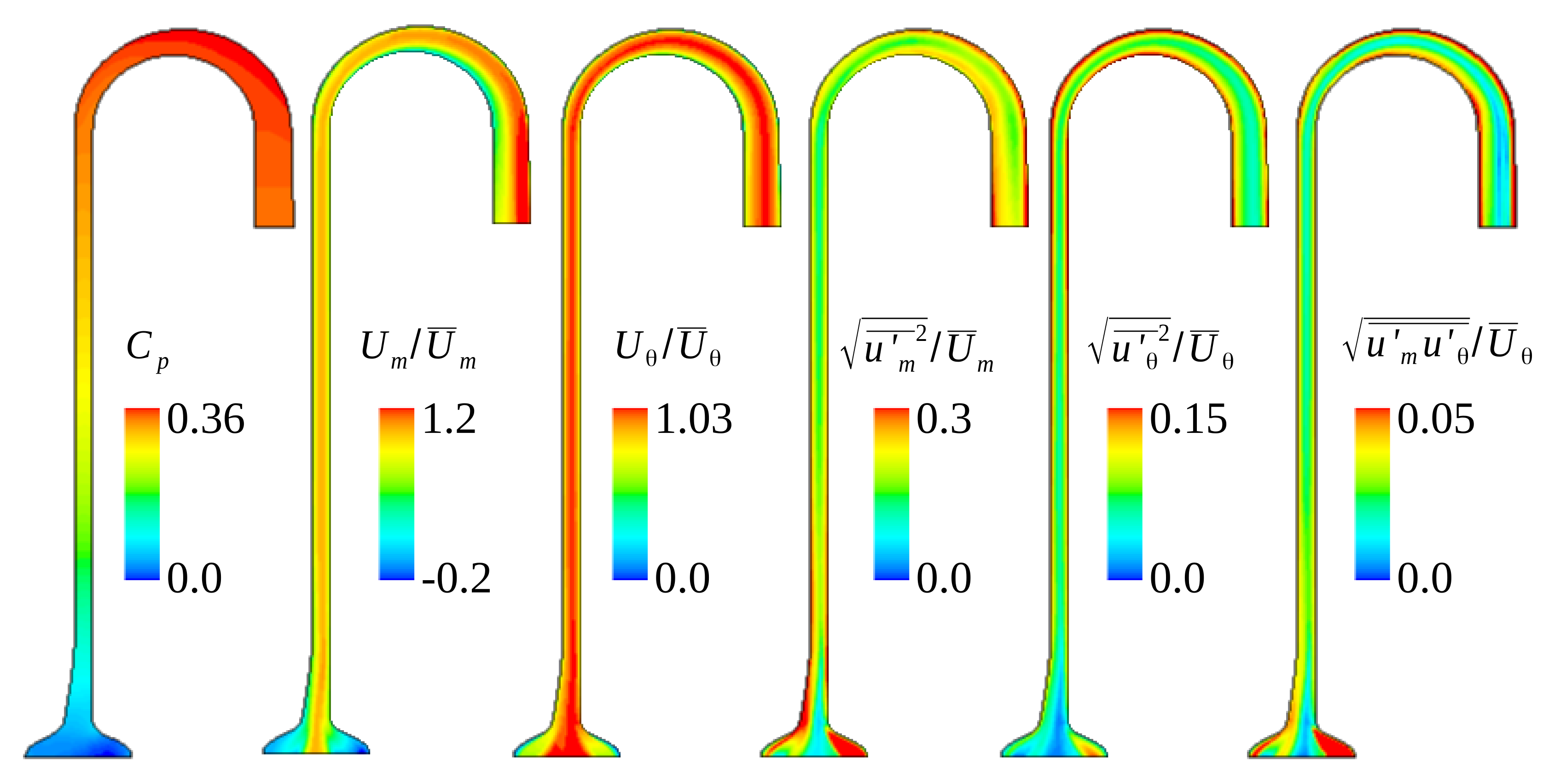
Based on the grid dependency assessment, the solution obtained with the fine grid resolution is chosen for further analysis. Figure 4 shows distributions on the side view of the time-averaged pressure, velocity components, and Reynolds stress levels, respectively, for the flow angle ${\alpha }_{IN}$ = 9.5${}^{\circ }$. The Reynolds stresses are scaled as a fluctuation intensity with respect to the mean local velocity. This velocity is obtained at the midway distance between the shroud and the hub and along the meridional coordinate. A characteristic pressure increase with a relatively steep gradient is seen until the top of the turnaround. After the top of the turnaround the cross section area decreases. This leads to a flow acceleration and thus to a static pressure decrease (see $C_p$ scalar distribution in Figure 4). At the turnaround bend a small pressure gradient is present in the wall-to-wall normal direction with slightly lower pressure on the hub side compared to the shroud side.

The time-averaged meridional and tangential velocity profiles, respectively, show a strong shear layer close to the inlet, which is due to the jet-like shape of the imposed inlet boundary profile. In the straight section the velocity components gradually approach the shape of a fully turbulent developed flow profile with high fluctuation levels close to the walls. To help see this more clearly the time-averaged meridional and tangential velocity profiles, respectively, are plotted in Figure 5 for different stations along the meridional direction, between $m=0.05$ and $m=0.8$. At meridional $m=0.6$, just prior the turnaround, the profiles approach an approximate self-similar solution.

Beyond $m=0.6$ both profiles are seen to tilt with reduced through flow close to the hub wall, an effect caused by the turnaround bend. Note that the time-averaged meridional velocity has a more extreme slope and indicates tendency of an inflection point between $m=0.7$ and $m=0.8$. This leads to increased fluctuations (root mean square) of this component ($u_m^{\prime }$). The steepness close to the shroud and hub at $m=0.6$ is compatible with the law of the wall. Therefore, wall modeling with lower resolution near the wall may lead to acceptable predictions. However, in the vicinity of the developing inflection point of the meridional velocity component there is evidence that wall modeling would not be acceptable and compromise prediction of potential boundary layer separation.

The fluctuation components of velocity in the meridional, the tangential as well as the co-variant direction, respectively, are depicted in Figure 4. A more detailed distribution of the fluctuation intensities is also depicted in Figure 5 for different meridional stations. Close to the inlet, peak fluctuation intensity is located close to the wall. In the middle of the channel, the peak values reduce and approach self-similarity. One explanation for this is the shape of the imposed boundary condition with the blades passing by creating high stress levels in the wake flow. Further downstream however, the intensity of the fluctuation reduces, which indicates turbulence decay. It is noted that the Reynolds stress anisotropy component exhibits a sudden growth at $m=0.7$ close to the hub wall (see Figure 4). However, this follows by a rapid recovery when the flow enters the area of favorable pressure gradient towards the outlet. In general the tangential stress level is dominant but the meridional and anisotropic stress components are not insignificant. This clarifies the importance of employing a numerical approach that can capture anisotropic features in diffuser flow.

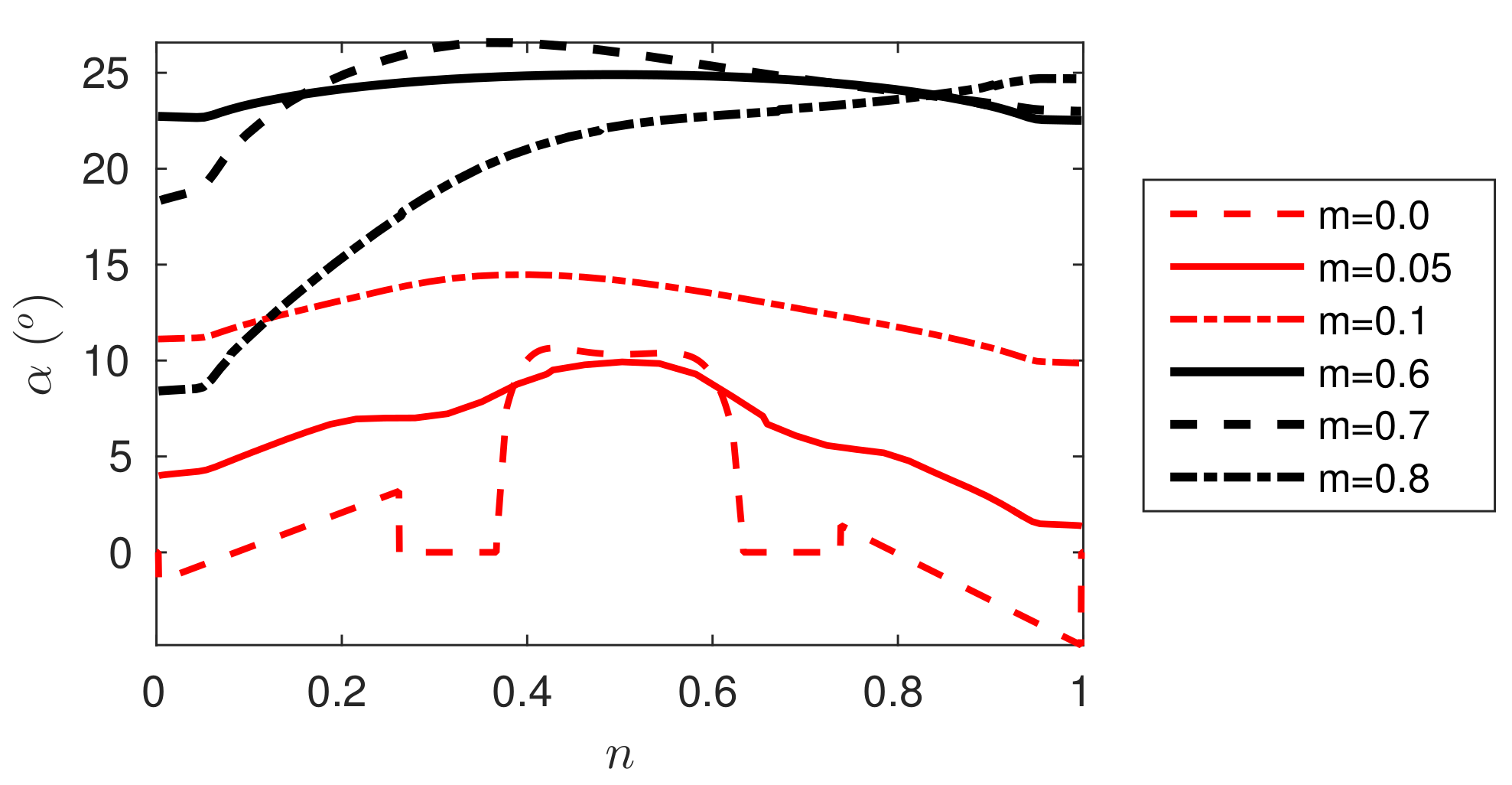
Assessment of the level of curvature requires a determination of the flow angle with respect to the tangent. This is presented in Figure 6 at different meridional stations.

The wall is said to be in a collateral state if the flow angle $\alpha =arctan(U_m/U_{\theta })$ is independent of the wall normal direction n. In other words, there would be a linear relationship between tangential and meridional velocities. It appears that this may hold in the straight diffuser section. A collateral state does not seem to hold past the turnaround at $m=0.7$. The figure shows evidence of a change in the flow angle as moving downstream with two different flow angles at the hub and shroud walls, respectively. In other words a smaller flow angle holds on the hub side as compared to the shroud side, and presenting a moderate gradient in between. This could be due to the concerted action of the turnaround bending effect and viscous effect near the wall, affecting the swirling motion of the core flow differently in the near wall regions associated with the hub and the shroud, respectively. In addition to this, the flow angle is seen to increase gradually towards the turnaround, which therefore gives a stabilizing effect. The increasing flow angle can also be linked with a loss of angular momentum due to viscous effect. In the area of the turnaround the flow angle decreases close to the hub side, which is associated with reduced through flow. This clearly leads to a destabilizing effect of the flow.

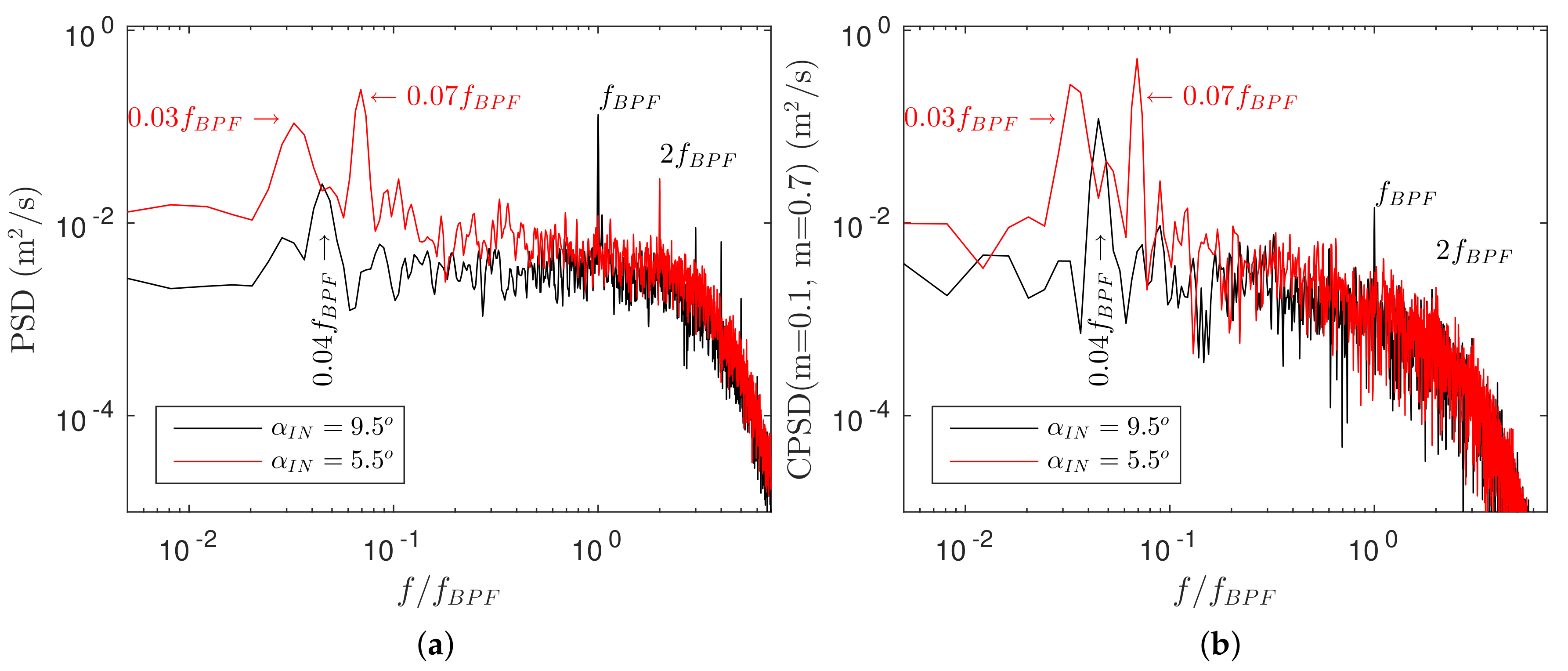
The presented results so far have only exposed statistics of the flow variables. A further assessment is carried out analyzing the power spectral density (PSD) of a monitored flow quantity of interest. Figure 7a shows PSD for the tangential velocity at $m=0.1$ in the mid of the diffuser channel, i.e., $n=0.5$. A combination of broadband and narrowband content is observed in the spectra. The tonality of the blade passing frequency including several higher harmonics is correctly captured with the numerical approach. In the low frequency end of the spectra for both inlet reference flow angles considered significant tonalities are revealed. For the larger flow angle case ${\alpha }_{IN}$ = 9.5${}^{\circ }$, one notable peak is observed at $0.04f_{BPF}$. For the lower flow angle case ${\alpha }_{IN}$ = 5.5${}^{\circ }$ two significant low frequency tonalities can be observed, one at $0.03f_{BPF}$ and the other at $0.07f_{BPF}$. The low frequency tonalities (i.e., $0.04f_{BPF}$ for the large flow angle case and $0.03f_{BPF}$ and $0.07f_{BPF}$ for the smaller flow angle case), correspond to flow modes with a periodic wave-like character. For the lower flow angle case the intensity level in the low to middle frequency range is seen to amplify. Moreover, the peak of the dominant narrowband feature, i.e., $0.07f_{BPF}$ for ${\alpha }_{IN}$ = 5.5${}^{\circ }$ as compared to $0.04f_{BPF}$ for ${\alpha }_{IN}$ = 9.5${}^{\circ }$, is shifted to a higher frequency relative to the shaft speed. It should be noted that the sample length corresponds to approximately 25 cycles of the low frequency tonality. Therefore, these features appear as broad peaks rather than sharp peaks in the point spectra. However, this could be improved with a more generous sampling length and hence simulation elapsed time. Although, if a harmonic signal is Gaussian shaped, the variation is not exactly sinusoidal.

Up to this point the numerical data elucidate two possible mechanisms for onset of the low frequency instability, i.e., one shear layer close to the inlet and a tendency of an inflection point in the turnaround section. To correlate these mechanisms with the rotating instability the point-to-point cross power spectral density (CPSD) of the tangential velocity fluctuation is presented in Figure 7b. The signals in the two different points show strong correlation at the rotating instability (i.e., $0.04f_{BPF}$ for ${\alpha }_{IN}$ = 9.5${}^{\circ }$) as well as at the blade passing frequency. The phase shift at the rotating instability frequency is approximately $-\chi$. This means that the signal closer to inlet is ahead approximately one blade-to-blade passage. For the smaller flow angle case ${\alpha }_{IN}$ = 5.5${}^{\circ }$ spatial coherency is also found in the low frequency range. There, the peak at $0.07f_{BPF}$ is seen to be more dominant over the peak at $0.03f_{BPF}$. Since their frequency ratio is not a whole number integer they are not harmonics of each other.

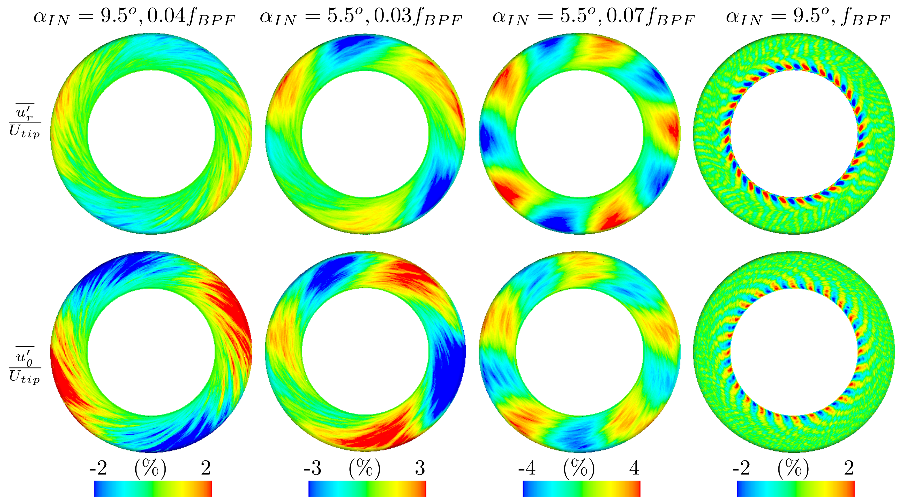
For a statistical characterization of the flow mode associated with the interesting narrowband instability a Fourier surface spectra analysis is performed of the velocity fluctuations $u_r^{\prime }$ and $u_{\theta }^{\prime }$ for every point distributed on a meridional surface located midway between the hub and the shroud, which follows the diffuser channel curvature. The number of cycles of the low frequency mode shape included in the surface spectra computation is limited to four and the result is presented in Figure 8 for the two different flow angles considered.

For a physical interpretation the intensities of the flow modes should be observed as a superposition on the mean flow ($U_i$) where the subscript i is a direction index. The real part of the flow mode spectra for the larger flow angle reveals two areas with negative intensity and two areas with positive intensity respectively, and distributed on opposing sides of each other. A positive radial intensity level is interpreted as outgoing flow and a negative level is a local inversion of the radial velocity component. The imaginary part (not included in the figure) is a phase shifted 90${}^{\circ }$ representation of the real part in the rotation direction of the shaft (clockwise in the figure). With the real and imaginary parts added together $u_i^{\prime }=\Re \left\{u_i^{\prime }\right\}cos\left(2\pi ft\right)-\Im \left\{u_i^{\prime }\right\}sin\left(2\pi ft\right)$ the shape of the mode is seen to rotate in the same direction as the impeller rotation. In other words, the flow mode can be described as a rotating instability consisting of two counter-rotating flow cells relative to each other. This qualitative description is in agreement with results of other research groups, e.g., [5,9]. The same feature can be attributed also to the lower flow angle (second and third columns) but with a larger number of rotating cells distributed evenly around the circumferential. The tonality at $0.03f_{BPF}$ for ${\alpha }_{IN}$ = 5.5${}^{\circ }$ (see Figure 7a) shows three disturbances (second column in Figure 8), whereas the other peak at $0.07f_{BPF}$ shows five rotating cells (third column in Figure 8).

One notable difference with the larger flow angle ${\alpha }_{IN}$ = 9.5${}^{\circ }$ as compared to the lower flow angle ${\alpha }_{IN}$ = 5.5${}^{\circ }$, can be seen in terms of their most dominant low frequency tonalities, respectively. That is $0.04f_{BPF}$ (first column in Figure 8) as compared to $f=0.07f_{BPF}$ (second column in Figure 8). For the coherent mode shape at $0.04f_{BPF}$ the intensity of the tangential fluctuating mode shape is more dominant compared to the radial fluctuating mode shape, which is rather weak in intensity. For peak $0.04f_{BPF}$ in the lower flow angle case, this is reversed, i.e., the radial fluctuation dominates over the tangential. The reason to this can be attributed to type and location of the outlet boundary condition for flow case ${\alpha }_{IN}$ = 5.5${}^{\circ }$. For this case a fraction of the cell face elements on the outlet were subjected to reversed flow, which means that those face elements can no longer be considered as a real outlet boundary. Under such situation the numerical solution may not be unique. Therefore, for the lower flow angle case there is a fraction of the outlet that violates the well-posedness criteria, see [22]. Strictly speaking, a solution to a problem that is not well-posed does not make sense, and so the numerical result for the lower flow angle case cannot be fully trusted. The remedy to this is to consider a repositioning of the outlet where the flow is purely outgoing. However, a common result is that the intensity level of the rotating disturbance reaches a peak at the top of the turnaround and with a growth point location prior to the turnaround.

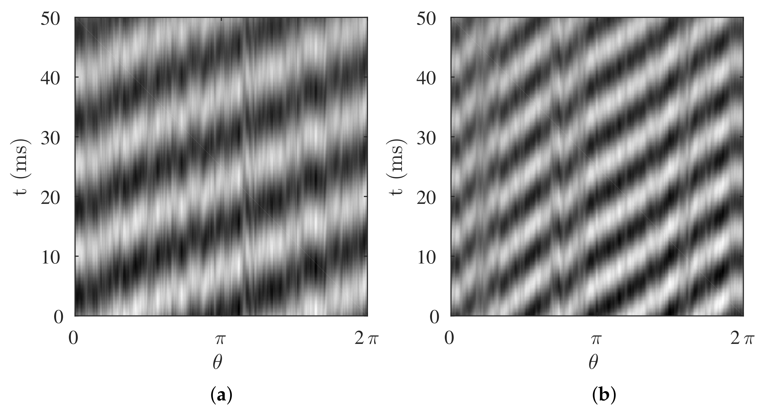
The propagation speed of the rotating stall cells can be analyzed using a space-time cross correlation. For this the tangential velocity fluctuating component $u_{\theta }^{\prime }$ is considered for all grid points, equidistant arranged along the circumferential direction at meridional $m=0.6$, between the hub and shroud midway in the diffuser channel. Among these points one is chosen as a reference located at twelve o’clock. Subsequently, the space-time cross correlation is computed as:

$$R(r_i,\Delta t)=\frac{<u^{\prime }(x_i,t)u^{\prime }(x_i+r_i,t+\Delta t)>}{\sqrt{<u^{\prime }(x_i,t){>}^2}\sqrt{<u^{\prime }(x_i+r_i,t+\Delta t){>}^2}}$$

(2)

The cross-correlation is then normalized and the result for flow angle cases $\alpha$ = 9.5${}^{\circ }$ and $\alpha$ = 5.5${}^{\circ }$ are presented in Figure 9.

The fluctuating tangential velocity component utilized in the space-time correlation is obtained by reconstruction of the most energetic Fourier surface spectra flow modes. The most energetic modes are determined from Figure 7. Thus, for flow angle case ${\alpha }_{IN}$ = 9.5${}^{\circ }$ the contributions from tonalities at $0.04f_{BPF}$ and $f_{BPF}$, respectively, are used. For the lower flow angle case ${\alpha }_{IN}$ = 5.5${}^{\circ }$, the contributions from $0.03f_{BPF}$, $0.07f_{BPF}$ and $f_{BPF}$ are used. A coherent pattern is observed with several inclined lines exhibiting strong correlation. This is directly linked with the propagation of the rotating cells. The slopes of the inclined lines are approximately constant and correspond to the local convection speed. For the large flow angle case, there are two disturbances along the circumference, which correlates with the two rotating stall cell structures in Figure 8, (i.e., $0.04f_{BPF}$ for ${\alpha }_{IN}$ = 9.5${}^{\circ }$). For the smaller flow angle case there are thus five disturbances, since there are five dominant rotating stall cell structures. For ${\alpha }_{IN}$ = 9.5${}^{\circ }$ the local convection speed is approximately 50% of the impeller speed. Now, the slope of the characteristic is different for ${\alpha }_{IN}$ = 5.5${}^{\circ }$, which is approximately 30% of the impeller speed. From Figure 7b and flow angle case ${\alpha }_{IN}$ = 9.5${}^{\circ }$ the tonality $0.04f_{BPF}$ is approximately one order larger than the $f_{BPF}$ tonality. Similarly, for flow angle case ${\alpha }_{IN}$ = 5.5${}^{\circ }$, the tonality at $0.07f_{BPF}$ is the most relevant. Therefore, only one set of inclined lines are appearing in each two-point cross-correlations (Figure 9).

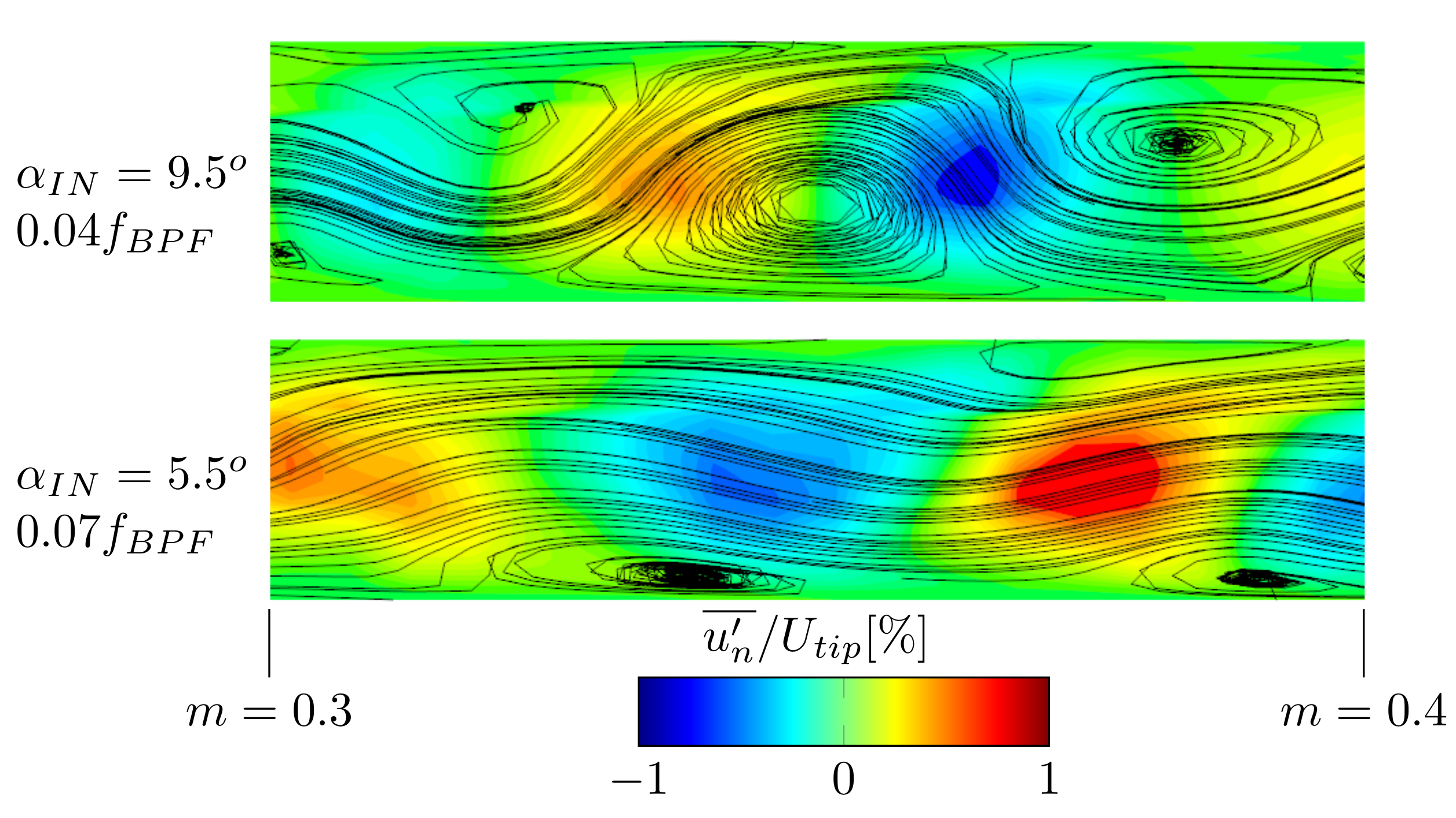
Another interesting observation in Figure 8 is that the radial and tangential velocity fluctuation distributions elucidate streaky elongated flow features, which propagate with the rotating stall mode. The length scale of the streaks is in the order of the diffuser channel width. Close to the inlet these features are located in the viscous sublayer rather in the core flow, which correlate with the amplified Reynolds stress levels close to the wall as shown in Figure 5. They can be identified as features carrying turbulent energy, which is an important characteristic of wall-bounded turbulence. Further out in the radial direction these stream-wise streaks grow with increased interaction and mixing with the core flow, see Figure 10. This partially motivates why the Reynolds stress distribution in the tangential direction becomes fuller in the mid of the diffuser channel.

Qualitatively, there is a resemblance with the stream-wise streaks found in the turbulent boundary layer in curved channel flow. However, in this case there is the added complication of an interaction with a rotating stall mode feature and an adverse pressure gradient. It is known that secondary flow instability can appear in a turbulent boundary layer over a curved channel wall. An important factor is when the boundary layer thickness is comparable to the radius of curvature. In such scenario, a centrifugal action creates a pressure variation across the boundary layer. This is said to lead to formation of longitudinal vortices [23]. In Figure 10, for the selected meridional section, for the larger flow angle case ${\alpha }_{IN}$ = 9.5${}^{\circ }$, two major rotating secondary flow structures are seen with counter clockwise rotation. These are located closer to the shroud wall. The other major vortex in between have a clockwise rotation and is located closer to the hub wall. Consequently, just ahead of the clockwise rotating vortex $\overline{u_n^{\prime }}$ is positive and just behind it $\overline{u_n^{\prime }}$ is negative. A similar sequence of updraft and downdraft of the wall normal velocity component between the hub and shroud walls can also be seen for the small flow angle case ${\alpha }_{IN}=$ = 5.5${}^{\circ }$. The onset of the instability can be estimated with the Görtler number, which is the ratio of centrifugal to viscous forces in the boundary layer. It is defined as:

$$G=\frac{U\theta }{\nu }{\left(\frac{\theta }{R}\right)}^{1/2}$$

(3)

where U-bulk flow velocity, $\theta$-momentum thickness, $\nu$-kinematic viscosity, and R-curvature radius of the wall. For the considered diffuser geometry this number exceeds 0.3, which is the critical limit for occurrence of the Görtler instability. This is one possible explanation for the coherent streaky features found superimposed on the rotating stall mode (see Figure 8).

4. Conclusions

The computation of the mean velocity components in a narrow vaneless diffuser at low flow angles suggests a possible connection between the tendency of boundary layer separation in an adverse pressure gradient and the tendency of flow circulation and propagation into a rotating stall consisting of counter-rotating flow structures. This is in agreement with published literature on the subject, e.g., [1,5]. For the diffuser geometry considered in this study a tendency of an inflection point was detected in the time-averaged meridional velocity profile close to the hub wall at the top of the turnaround location. This correlates with a sudden reduction in the near-wall stress level in the near-wall region, which is indicative of approaching boundary layer separation.

An emerging feature of the rotating stall instability is the formation of counter-rotating flow structures. Such features of the flow causes unsteady effects on the turbulence structures residing in the boundary layer. One important perturbation mechanism is linked with the pressure gradient developed and the impact of the streamwise curvature. This conclusion is associated with the peak Reynolds stress level moving closer to the core flow and the response in the near-wall hub region, where flow blockage occurs. Another interesting feature is the characteristic turbulent streaks found in the turbulent boundary layer, which are being convected with the rotating stall instability. Those are turbulent energy carrying features. They were found to form longitudinal vortices with length scale in the order of the diffuser channel width. These features share resemblance with the secondary flow instability in turbulent boundary layers subjected to curvature effect.

A strong shear-layer is located close to the inlet, which is due to the considered shape of the imposed boundary condition. This correlates with high Reynolds stress levels and is another possible mechanism for the onset of the rotating instability which is seen to grow further downstream in the diffuser. The point-to-point cross-correlation was computed in order to determine the phase differences between the dominant flow modes, i.e., the rotating instability mode and the blade passing frequency mode. This is understood to be a convolution over a finite period with similar notion to a Fourier transform with assumption of periodicity. Consequently, all notions of causality are lost and one can no longer refer to driver and response signals, but only signals which are correlated. Therefore, it is challenging to say which signal drives which. However, the numerical result shows a strong coherence between the shear-layer instability close to the inlet and the developing instability prior to the turnaround location.